Automatic Modulation Recognition Based on Adaptive Wavelet Enhancement and Dynamic Graph Construction

Abstract

Automatic modulation recognition (AMR) is essential for cognitive radio and intelligent wireless communication, yet its performance degrades markedly under low signal-to-noise ratio (SNR) conditions because weak local structures are corrupted and class boundaries become less separable. To address this problem, we propose ADGNet, an automatic modulation recognition network based on adaptive wavelet enhancement and dynamic graph construction. ADGNet adopts a dual-branch architecture in which the main branch extracts time-domain amplitude–phase features from raw in-phase/quadrature sequences, while the auxiliary branch combines short-time Fourier transform features with adaptive wavelet features to capture complementary frequency–energy distributions and multi-scale transient details. A dual-domain adaptive encoder then recalibrates and fuses the two branches, suppressing redundant and noise-contaminated responses. In addition, a G2 dynamic topology module constructs sample-adaptive top-k adjacency matrices from node features and fuses them with the original graph structure to improve temporal relation modeling. Experiments on RadioML2016.10a and RadioML2016.10b show average accuracies of 64.23% and 69.69%, respectively. On RadioML2016.10b, ADGNet achieves 63.48% average accuracy from −12 dB to 0 dB, compared with 59.51% for the baseline. With approximately 0.13 million parameters, ADGNet provides a favorable balance between low-SNR robustness and model complexity.

1. Introduction

Automatic modulation recognition (AMR) is a key technique in intelligent wireless communication systems. Its objective is to identify the modulation type of a received signal without prior knowledge of transmitter parameters, modulation parameters, channel state information, or synchronization information. As an intermediate process between signal detection and demodulation, AMR is widely used in spectrum monitoring, cognitive radio, non-cooperative communication, electronic reconnaissance, and dynamic spectrum access [1,2].

With the development of broadband, heterogeneous, and intelligent wireless systems, received signals are frequently affected by multipath fading, carrier frequency offset, phase offset, sampling-rate offset, and additive noise. These impairments are particularly severe under low signal-to-noise ratio (SNR) conditions. In such cases, the amplitude–phase distribution, local transient structure, and temporal correlation of modulation signals are heavily disturbed by noise, which leads to blurred decision boundaries between different modulation classes. Therefore, improving robust representation learning and generalization capability under low-SNR conditions remains an important problem in AMR.

Traditional AMR methods can generally be divided into likelihood-based methods and feature-based methods [3]. Likelihood-based methods usually depend on accurate channel models, noise distributions, and synchronization information. Although these methods can achieve good decision performance under ideal assumptions, they usually suffer from high computational complexity and limited applicability in practical non-cooperative scenarios. Feature-based methods classify modulation signals using handcrafted features, such as higher-order cumulants, cyclic spectra, instantaneous amplitude, instantaneous phase, and constellation diagrams. These methods have a certain degree of interpretability, but their performance depends strongly on expert-designed features and tends to degrade under low SNR, multipath fading, and frequency offset.

In recent years, deep learning has become an important approach for AMR because of its end-to-end feature learning capability. Convolutional neural networks can directly extract local waveform features [4,5] from raw I/Q sequences, while CNN-LSTM models further combine convolutional representations with temporal dependency modeling [6,7]. Transformer-based and hybrid temporal networks improve long-range dependency modeling and global contextual representation [8,9,10]. These studies have improved AMR performance significantly. However, under extremely low-SNR conditions, weak discriminative details are still easily submerged by noise, and the ability of existing models to capture local non-stationary structures remains insufficient.

Zhang et al. introduced an adaptive wavelet network for automatic modulation classification, showing that learnable wavelet-based representations can provide multi-scale descriptions of received signals [11]. Subsequent studies further investigated adaptive lightweight wavelet decomposition, wavelet-domain feature extraction, and denoising representation learning for modulation recognition [12,13,14]. These methods demonstrate the potential of learnable multi-scale analysis for preserving transient amplitude, phase, and frequency variations that are easily corrupted by noise. However, existing wavelet-based AMR methods mainly focus on front-end feature enhancement or denoising, while the joint modeling of local multi-scale characteristics, complementary cross-domain information, and sample-dependent structural relations remains insufficient. This limitation motivates the integration of wavelet-inspired local-detail enhancement with adaptive feature fusion and graph-based relation modeling in ADGNet.

Multi-domain feature fusion provides another way to improve modulation representation. Raw I/Q sequences retain time-domain amplitude and phase variations, whereas time–frequency representations describe local frequency–energy distributions. Existing studies have explored multi-domain fusion, joint modeling of I/Q and time–frequency features, and multimodal Transformer architectures [15,16,17]. These approaches demonstrate the complementarity of heterogeneous signal representations. However, direct concatenation, fixed weighting, or shared fusion mechanisms may not adequately account for variations in feature reliability across different samples and SNR conditions. When the auxiliary representation is strongly contaminated by noise, indiscriminate fusion may introduce redundant or unreliable responses into the subsequent feature extractor. Therefore, an adaptive mechanism that independently recalibrates different feature domains before fusion is desirable for low-SNR modulation recognition.

Graph neural networks provide a natural framework for modeling structural dependencies among temporal segments of modulation signals. AvgNet adaptively maps radio time series into visibility graphs and combines graph representations with a modified DiffPool classifier [18]. STF-GCN models adaptive correlations among multi-domain modulation features [19], whereas CTGNet integrates convolutional, Transformer, and graph-based representations to capture complementary local, global, and structural information [20]. More recently, an input-dependent dynamic graph architecture has been introduced for modulation classification [21].

Adaptive graph-learning mechanisms have also been investigated in related time-series tasks. Graph WaveNet learns latent dependencies from trainable node embeddings and combines them with predefined graph supports [22], while MTGNN constructs sparse directed graphs through adaptive relation learning and top-k neighbor selection [23]. These studies show that learnable topology construction can provide an effective alternative when predefined graph relations are incomplete or insufficiently flexible.

Nevertheless, ADGNet focuses specifically on sample-dependent temporal relations in modulation signals. For each input sample, the G2 module constructs a sparse top-k adjacency matrix from temporal node features and integrates it with the original graph structure before hierarchical graph reasoning. In this way, the graph topology can respond to variations in node relationships caused by noise and channel distortion rather than relying solely on a predefined construction rule.

To address these problems, this paper proposes an automatic modulation recognition network based on adaptive wavelet enhancement and dynamic graph construction, named ADGNet. The main contributions are summarized as follows.

(i) An adaptive wavelet front-end is introduced to enhance non-stationary local details in modulation signals. By learning multi-scale high-frequency detail representations, the model improves its ability to capture weak discriminative features under low-SNR conditions.

(ii) A dual-domain adaptive encoder is designed to recalibrate and fuse the main I/Q features and auxiliary features composed of STFT and adaptive wavelet representations. This mechanism enables sample-adaptive feature selection and reduces the influence of redundant or noise-contaminated auxiliary responses.

(iii) A G2 dynamic topology construction module is developed to generate a sample-adaptive top-k adjacency matrix from node features and fuse it with the original adjacency relationship. This module enhances structural relation modeling among temporal segments and improves recognition robustness under complex noisy conditions.

The effectiveness of the proposed method is verified on the RadioML2016.10a and RadioML2016.10b datasets. The experimental results show that ADGNet achieves higher average recognition accuracy, stronger low-SNR recognition capability, and a favorable balance between model complexity and recognition performance.

2. Signal Model and Feature Representation

Automatic modulation recognition can be formulated as a pattern classification problem for finite-length received sequences. For a given modulation class, the ideal baseband symbols usually have relatively stable amplitude, phase, or frequency variation patterns. However, in practical wireless channels, the received sequence is affected by channel convolution, frequency offset, phase rotation, and random noise. These factors shift and disperse the original modulation structure in the observation space.

Let the ideal complex baseband modulation sequence of length N be denoted by

$$s={\left[s_0,s_1,\dots ,s_{N-1}\right]}^T$$

(1)

After wireless channel transmission, the received sequence can be uniformly expressed as

$$r=D(\Delta f,\theta )Hs+w$$

(2)

where $H$ represents the linear channel transformation caused by multipath propagation, $D(\mathsf{\Delta }f,\theta )$ represents the complex rotation induced by the carrier-frequency offset $\Delta f$ and phase offset $\theta$, and $w$ denotes complex additive noise. Compared with explicitly expanding each channel parameter, this formulation emphasizes the overall variation of the received signal in the feature space.

Since most standard neural network implementations cannot directly process complex-valued signals, the received complex sequence is usually mapped into a real-valued two-channel representation:

$$R_{\mathrm{IQ}}(r)=\left[\begin{array}{c}\mathrm{Re}(r)\\ \mathrm{Im}(r)\end{array}\right]\in {ℝ}^{2\times N}$$

(3)

where $\mathrm{Re}(r)$ and $\mathrm{Im}(r)$ denote the real and imaginary parts of the received complex sequence, respectively.

This representation preserves the amplitude–phase structure of the original signal and maintains local variation relationships among sampling points. For PSK signals, discriminative information mainly lies in phase states and their transition patterns. For QAM signals, discriminative information depends on both amplitude levels and phase distributions. For FSK signals, the sequence correlation caused by frequency variation is more important. Therefore, I/Q representation is suitable as the basic input for modeling the original time-domain structure of modulation signals [3].

However, low SNR weakens the local stability of I/Q sequences. Taking high-order QAM as an example, noise perturbation reduces the separability between different amplitude levels and blurs constellation boundaries. For PSK signals, noise causes phase-state deviations within short time windows. For analog modulation signals, low-energy segments can easily be dominated by noise. Therefore, relying only on I/Q sequences may cause the model to overfit local random disturbances while ignoring stable frequency structures across temporal segments.

To obtain local frequency-structure information, the received signal can be projected onto a set of local time–frequency bases [24]. Let ${\mathrm{g}}_{\mathrm{m},\mathrm{k}}\left[\mathrm{n}\right]$ denote the local time–frequency analysis basis centered at the $\mathrm{m}$-th time window and the $\mathrm{k}$-th frequency bin. The response of the received signal in this local time–frequency unit can be expressed as

$$\mathcal{T}(m,k)=⟨r[n],g_{m,k}[n]⟩$$

(4)

and the corresponding local magnitude distribution is given by

$$\mathcal{E}(m,k)=\left|\mathcal{T}(m,k)\right|$$

(5)

where $⟨\cdot ,\cdot ⟩$ denotes the inner-product operation, which measures the response of the signal to the local analysis basis. Based on the above analysis, the proposed model is designed around three aspects: local-detail enhancement, cross-domain complementary fusion, and node-relation modeling.

3. Proposed Method

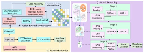
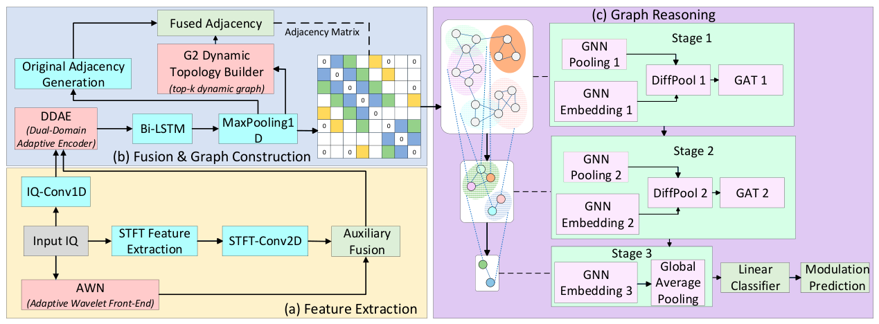
This paper proposes an automatic modulation recognition network based on adaptive wavelet enhancement and dynamic graph construction, named ADGNet. The overall architecture is shown in Figure 1. The proposed model takes a (2 × 128) I/Q sequence as input and consists of a main I/Q branch, an auxiliary feature branch, a dual-domain adaptive fusion module, a dynamic topology construction module, and a hierarchical graph reasoning module.

Figure 1. Architecture of the proposed modulation recognition network. Colored backgrounds distinguish feature extraction (yellow), fusion and graph construction (blue), and graph reasoning (purple). Dashed lines indicate the hierarchical information flow between successive graph-reasoning stages.

The main I/Q branch is used to extract raw time-domain amplitude–phase features from the received signal. The auxiliary branch combines short-time Fourier transform (STFT) time–frequency features and adaptive wavelet network (AWN) features to supplement local frequency–energy distributions and multi-scale non-stationary details. In the feature fusion stage, the dual-domain adaptive encoder (DDAE) recalibrates and fuses the main I/Q features and auxiliary features, thereby improving the use of complementary cross-domain information. In the graph reasoning stage, the G2 dynamic topology construction module generates a sample-adaptive adjacency matrix according to node features and fuses it with the original adjacency matrix, providing structural constraints for hierarchical graph reasoning. This design enables ADGNet to improve low-SNR modulation recognition from both multi-domain feature representation and node-relation modeling.

3.1. Adaptive Wavelet Enhancement and Dual-Domain Feature Fusion

Under low-SNR conditions, the discriminative information of modulation signals often appears as fine-grained local structures, such as phase transitions in PSK signals, amplitude-level variations in QAM signals, and short-time frequency changes in FSK signals. These structures are highly non-stationary in raw I/Q sequences and are easily disturbed by random noise. STFT can provide the frequency–energy distribution within a local time window, but its window function and transform basis are fixed. Therefore, it lacks adaptability to local abrupt changes and scale variations in different signal samples.

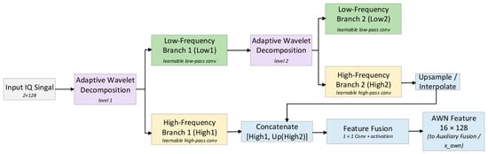
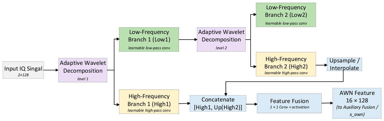
To address this limitation, this paper introduces an adaptive wavelet network (AWN) front-end into the auxiliary branch to enhance non-stationary local details. The structure of AWN is shown in Figure 2. Wavelet analysis has excellent time–frequency localization and multi-scale analysis capability, which is suitable for capturing transient phase jumps and amplitude mutations of noisy modulation signals. Standard discrete wavelet transform (DWT) relies on manually fixed low-pass and high-pass filter banks to realize signal decomposition:

$$L=x\ast g, H=x\ast h, \tilde{L}=L\downarrow 2$$

(6)

where $g$ and $h$ denote fixed low-pass and high-pass wavelet filters, $L$ is the low-frequency approximate component after convolution, $H$ is the high-frequency detail component, and $\downarrow 2$ represents 2-fold downsampling.

Figure 2. Structure of the adaptive wavelet front-end. At the first level, the input I/Q sequence is processed by independent learnable low-frequency and high-frequency convolutional kernels to obtain $L^{(1)}$ and $H^{(1)}$. The low-frequency feature is downsampled and decomposed again to obtain the second-scale detail feature $H^{(2)}$. After temporal interpolation, $H^{(1)}$ and ${\widehat{H}}^{(2)}$ are concatenated and fused to produce the 16 × 128 AWN representation.

Unlike a conventional DWT with fixed analysis filters, the proposed AWN employs learnable one-dimensional convolutional kernels at two decomposition levels. Let

$$X\in {ℝ}^{B\times 2\times T}$$

(7)

denote a batch of input I/Q sequences, where B is the batch size and T = 128 is the sequence length. The learnable low-frequency and high-frequency kernels at decomposition level $l\in \{1,2\}$ are denoted by $W_L^{(l)}$ and $W_H^{(l)}$, respectively.

At the first decomposition level, the input sequence is processed as

$$L^{(1)}=X\ast W_L^{(1)}$$

(8)

$$H^{(1)}=X\ast W_H^{(1)}$$

(9)

where $\ast$ denotes one-dimensional convolution. $W_L^{(1)}$ and $W_H^{(1)}$ denote the learnable low-frequency and high-frequency convolutional kernels at the first decomposition level, respectively, and $L^{(1)}$ and $H^{(1)}$ denote the corresponding first-level smooth and detail features.

The first-level low-frequency feature is then downsampled using average pooling:

$${\tilde{L}}^{(1)}=\mathrm{AvgPool}\left(L^{(1)};k=2,s=2\right)$$

(10)

where $k$ and $s$ denote the pooling-kernel size and stride, respectively. The sequence length of ${\tilde{L}}^{(1)}$ is therefore $\mathrm{T}/2$.

At the second decomposition level, two independent learnable convolutional kernels are applied to the downsampled low-frequency feature:

$$L^{(2)}={\tilde{L}}^{(1)}\ast W_L^{(2)}$$

(11)

$$H^{(2)}={\tilde{L}}^{(1)}\ast W_H^{(2)}$$

(12)

where $W_L^{(2)}$ and $W_H^{(2)}$ denote the learnable low-frequency and high-frequency convolutional kernels at the second decomposition level, respectively; $L^{(2)}$ denotes the second-level smooth feature, and $H^{(2)}$ denotes the second-scale detail feature extracted from the downsampled low-frequency representation. Since $H^{(2)}$ has a temporal length of $\mathrm{T}/2$, it is linearly interpolated to the original sequence length T before multi-scale feature fusion:

$${\widehat{H}}^{(2)}=\mathrm{Interp}\left(H^{(2)},T\right)$$

(13)

where $\mathrm{Interp}(\cdot ,T)$ denotes linear interpolation to the target temporal length $T$, and ${\widehat{H}}^{(2)}$ denotes the temporally aligned second-scale detail feature. The first-scale detail feature $H^{(1)}$ and the aligned second-scale detail feature ${\widehat{H}}^{(2)}$ are then concatenated along the channel dimension and mapped to the AWN output:

$$F_{\mathrm{AWN}}=f_w\left(\mathrm{Cat}\left[H^{(1)},{\widehat{H}}^{(2)}\right]\right)$$

(14)

where $\mathrm{Cat}[\cdot ]$ denotes channel-wise concatenation and $f_w(\cdot )$ denotes the subsequent 1 × 1 convolutional fusion mapping. The resulting AWN representation satisfies $F_{\mathrm{AWN}}\in {ℝ}^{B\times 16\times 128}$.

The AWN follows a two-level wavelet-inspired decomposition process by progressively separating smooth and detail representations. However, it does not impose the orthogonality, perfect-reconstruction, or fixed-filter constraints of a conventional DWT. Therefore, it is more precisely described as a learnable wavelet-inspired front-end rather than as an exact discrete wavelet transform.

In the auxiliary branch, STFT features and AWN features have different information preferences. STFT features reflect local frequency–energy distributions and are suitable for describing frequency-domain structures within short time windows. AWN features emphasize multi-scale local details and are suitable for capturing non-stationary modulation variations. The two types of features are fused to obtain the auxiliary representation:

$$F_{\mathrm{Aux}}=f_{\mathrm{Aux}}\left(\mathrm{Cat}\left(F_{\mathrm{STFT}},F_{\mathrm{AWN}}\right)\right)$$

(15)

where $F_{\mathrm{STFT}}$ and $F_{\mathrm{AWN}}$ denote the outputs of the STFT branch and the adaptive wavelet branch, respectively, and $f_{\mathrm{Aux}}(\cdot )$ denotes the auxiliary feature-fusion mapping.

This operation does not simply increase the number of input channels. Instead, it combines fixed time–frequency analysis with learnable wavelet-detail enhancement, allowing the auxiliary branch to obtain both frequency–energy description capability and local-detail enhancement capability.

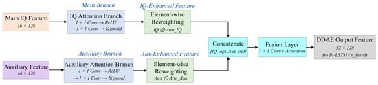
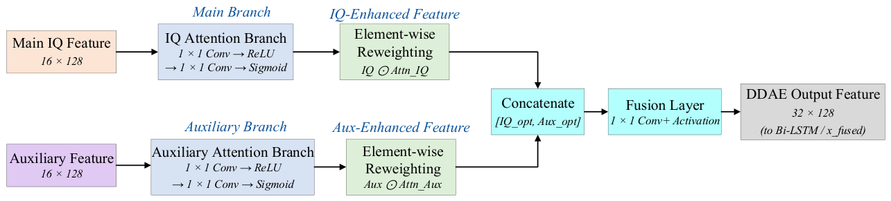
However, the reliability of the main I/Q features and auxiliary features varies with the SNR level and modulation type. If these two types of features are directly concatenated, redundant responses or noise interference may be introduced. To address this problem, inspired by feature recalibration [25], this paper designs a dual-domain adaptive encoder (DDAE). Its structure is shown in Figure 3.

Figure 3. Structure of the dual-domain adaptive encoder.

Let $F_{\mathrm{IQ}}$, $F_{\mathrm{Aux}}\in {ℝ}^{B\times 16\times 128}$ denote the main-branch I/Q feature and the auxiliary feature, respectively. Two independent attention mappings are used to generate domain-specific recalibration weights:

$$M_{\mathrm{IQ}}=\sigma \left({\psi }_{\mathrm{IQ}}\left(F_{\mathrm{IQ}}\right)\right),\hspace{1em}\hspace{1em}{M}_{\mathrm{Aux}}=\sigma \left({\psi }_{\mathrm{Aux}}\left(F_{\mathrm{Aux}}\right)\right)$$

(16)

where ${\psi }_{\mathrm{IQ}}(\cdot )$ and ${\psi }_{\mathrm{Aux}}(\cdot )$ are independent attention mappings for the main and auxiliary domains, respectively, and $\sigma (\cdot )$ is the sigmoid activation function. The resulting attention matrices are dimensionally compatible with their corresponding input features.

The two domain features are recalibrated as

$${\widehat{F}}_{\mathrm{IQ}}=F_{\mathrm{IQ}}\odot M_{\mathrm{IQ}}, {\widehat{F}}_{\mathrm{Aux}}=F_{\mathrm{Aux}}\odot M_{\mathrm{Aux}}$$

(17)

where $\odot$ denotes element-wise multiplication. The independent attention mappings allow the model to suppress unreliable responses in one branch without forcing the other branch to use the same recalibration pattern.

Finally, the recalibrated features are concatenated along the channel dimension and fused as

$$F_D=f_D\left(\mathrm{Cat}\left[{\widehat{F}}_{\mathrm{IQ}},{\widehat{F}}_{\mathrm{Aux}}\right]\right)$$

(18)

where $f_D(\cdot )$ denotes the convolutional fusion mapping and $F_D\in {ℝ}^{B\times 32\times 128}$.

Thus, DDAE performs sample-dependent recalibration separately in the I/Q and auxiliary domains before cross-domain fusion.

3.2. Dynamic Graph Construction and Graph Reasoning

Modulation signals have clear temporal correlations. Their class differences are reflected not only in the amplitude–phase responses of local sampling segments, but also in the association patterns among different temporal segments. For example, PSK signals depend on phase-state transitions, FSK signals are characterized by frequency-trajectory variations, and QAM signals are affected by both amplitude levels and phase distributions. Therefore, relying only on convolutional local feature extraction or recurrent sequential dependency modeling is still insufficient for fully capturing complex internal node relations in modulation signals.

To further enhance structural relation modeling, this paper introduces a graph reasoning mechanism based on temporal features. Specifically, the dual-domain fused feature is first rearranged into a temporal sequence and processed by a two-layer bidirectional long short-term memory (Bi-LSTM) network. The fused feature before the recurrent module has a size of $B\times 32\times 128$, and is transposed to $B\times 128\times 32$, where the 128 positions correspond to the original temporal sampling locations. The hidden size of the Bi-LSTM is set to 32 for each direction. Therefore, concatenating the forward and backward hidden states produces a 64-dimensional representation at each temporal position:

$$H_{\mathrm{BiLSTM}}\in {ℝ}^{B\times 128\times 64}$$

(19)

where $H_{\mathrm{BiLSTM}}$ denotes the output feature tensor of the two-layer bidirectional LSTM, $B$ is the batch size, 128 denotes the number of temporal positions, and 64 denotes the concatenated hidden dimension of the forward and backward LSTM directions.

A one-dimensional max-pooling operation with kernel size 4 and stride 4 is subsequently applied along the feature dimension rather than the temporal dimension. This operation reduces the feature dimension from 64 to 16 while preserving all 128 temporal positions:

$$X=\mathrm{MaxPool}1\mathrm{D}\left(H_{\mathrm{BiLSTM}};k=4,s=4\right)\in {ℝ}^{B\times 128\times 16}$$

(20)

where $X$ denotes the graph-node feature matrix obtained after feature-dimension max pooling, and the dimensions 128 × 16 correspond to 128 temporal nodes with a 16-dimensional feature vector for each node.

Consequently, each of the 128 temporal positions is treated as one graph node, and each node is represented by a 16-dimensional feature vector. For an individual sample, the resulting node-feature matrix is therefore $X\in {ℝ}^{128\times 16}$. The graph construction module subsequently models the relationships among these 128 temporal nodes.

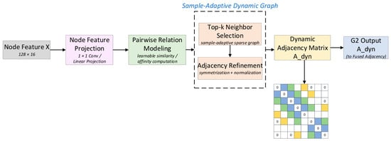
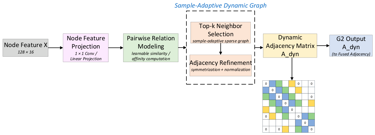
Traditional graph neural networks commonly perform message propagation over a predefined graph structure [26]. However, under low-SNR conditions, noise disturbance, phase offset, and local distortion may change the effective internal node relations of different samples. If a fixed topology is still used, invalid information may propagate between noise-dominated nodes and discriminative nodes. To address this problem, this paper designs a G2 dynamic topology construction module, as shown in Figure 4.

Figure 4. Structure of the G2 dynamic topology construction module. The globally shared learnable coefficient α balances the original rule-based adjacency and the sample-specific dynamic adjacency, while the dynamic topology is generated independently from the node features of each input sample.

The G2 module mainly consists of three parts: original adjacency generation, dynamic topology construction, and adjacency matrix fusion. The original adjacency matrix provides stable basic connections and ensures that the graph structure has a fundamental topological constraint. The dynamic topology constructor calculates node correlations according to the node features of the current sample and retains the top (k) most relevant neighbors for each node [21], forming a sample-adaptive dynamic graph. The dynamic adjacency matrix can be expressed as

$${\left(A_{\mathrm{dyn}}\right)}_{ij}=\left\{\begin{array}{ll}{S}_{ij},\hfill & j\in \mathrm{TopK}\left(S_{i,:}\right)\hfill \\ 0,\hfill & \mathrm{otherwise}.\hfill \end{array}\right.$$

(21)

where $S_{ij}$ denotes the correlation between nodes $i$ and $j$, and $\mathrm{TopK}(S_{i,:})$ denotes the index set of the $k$ largest elements in the $i$-th row of the similarity matrix $S$. This sparse connection strategy reduces irrelevant edges and noise edges, enabling the graph structure to focus more on discriminative node relations in the current sample.

To avoid structural fluctuation caused by relying entirely on the dynamic adjacency matrix, this paper further fuses the original adjacency matrix and the dynamic adjacency matrix as

$$\widehat{A}=\mathrm{RowNorm}\left(\alpha A_{\mathrm{ori}}+\left(1-\alpha \right)A_{\mathrm{dyn}}+I\right)$$

(22)

where $A$ denotes the final fused adjacency matrix, $A_{\mathrm{orig}}$ denotes the original rule-based adjacency matrix, $A_{\mathrm{dyn}}$ denotes the sample-adaptive dynamic adjacency matrix, I denotes the identity matrix used to introduce self-loops, $\alpha$ is a globally shared learnable fusion coefficient initialized to 0.5, and $\mathrm{RowNorm}(\cdot )$ denotes row-wise normalization.

It is worth noting that sample-level adaptability of the graph module is realized via $A_{\mathrm{dyn}}$ instead of the shared coefficient $\alpha$. A unique similarity topology is generated for each sample according to its node features, while $\alpha$ only balances the weight of the original rule-based adjacency $A_{\mathrm{orig}}$ and the sample-specific dynamic graph $A_{\mathrm{dyn}}$. As each sample holds its exclusive $A_{\mathrm{dyn}}$, the fused adjacency $A_{\mathrm{fused}}$ varies inherently even with a global $\alpha$. The coefficient $\alpha$ is implemented as a globally shared learnable scalar initialized to 0.5. Therefore, $\alpha$ itself is not sample-dependent; it only controls the global balance between the two adjacency constructions. Sample-dependent graph variation is introduced through adjacency matrices computed from the node features of each input sample.

The original rule-based adjacency provides a structured local-relation prior, whereas the learned dynamic adjacency introduces additional sample-specific topology adaptation.

After the fused adjacency matrix is obtained, a hierarchical graph reasoning module is used to aggregate node features. As shown in Figure 4, the first stage takes 128 nodes as input. A graph neural network pooling module learns the node assignment relationship, and a graph neural network embedding module extracts node embeddings. Then, differentiable pooling (DiffPool) [27] is used to compress the graph structure from 128 nodes to 32 nodes. This process aggregates fine-grained temporal segments into higher-level local substructures and reduces the influence of redundant nodes on classification.

Subsequently, a graph attention network (GAT) [28] is used to conduct weighted information interaction among the compressed nodes. The attention mechanism enables the model to assign different importance weights to neighboring nodes and highlight key connections related to modulation classes. In the second stage, graph pooling and graph attention are further applied to compress the number of nodes from 32 to 8, thereby forming a more compact graph-level discriminative representation.

Finally, global average pooling is used to obtain the graph-level feature (h), and a linear classifier outputs the modulation-class probability distribution:

$$p=\mathrm{Softmax}(W_{c}h+b_c)$$

(23)

where $h$ denotes the graph-level feature obtained by global average pooling, $W_c$ and $b_c$ denote the classifier weight matrix and bias vector, respectively, and $p$ denotes the predicted probability distribution over the modulation classes. During training, the cross-entropy loss function is adopted to optimize the classification network:

$${\mathcal{L}}_{CE}=-{\displaystyle \sum _{c=1}^C{y}_c}\log p_c$$

(24)

where ${\mathcal{L}}_{CE}$ denotes the cross-entropy loss, $C$ denotes the number of modulation classes, $y_c$ denotes the ground-truth indicator for class c, and $p_c$ denotes the predicted probability assigned to class $c$. Through G2 dynamic topology construction and hierarchical graph reasoning, ADGNet transforms temporal features into graph-level discriminative representations with structural constraints, thereby improving the recognition ability for complex modulation signals under low-SNR conditions.

4. Experimental Setup

The RadioML2016.10a and RadioML2016.10b datasets are used to evaluate the proposed method [29]. RadioML2016.10a is a synthetic modulation recognition dataset generated using GNU Radio. It contains 220,000 signal examples from 11 modulation classes, including eight digital modulations and three analog modulations. The SNR ranges from −20 to 18 dB with an interval of 2 dB. Each example contains 128 complex baseband samples and is stored as a 2 × 128 real-valued array corresponding to the in-phase and quadrature components. The dataset-generation code specifies a sampling rate of 200 kHz. For the digital modulation classes, the transmitter uses eight samples per symbol; this parameter is not applicable to the analog modulation classes. The documented channel model includes sample-rate offset, center-frequency offset, Rician selective fading with multipath, and additive white Gaussian noise.

RadioML2016.10b contains 1,200,000 examples from ten modulation classes and uses the same 2 × 128 input representation and SNR range. However, its complete signal-generation parameters are not fully described in publicly available source materials. Therefore, Table 1 reports only directly verifiable dataset characteristics, while undocumented parameters are marked as not publicly specified rather than being treated as confirmed values. The main characteristics of both datasets are summarized in Table 1.

Table 1. Main characteristics of the RadioML2016.10a and RadioML2016.10b datasets.

Parameter	RadioML2016.10a	RadioML2016.10b
Number of modulation classes	11	10
Digital modulations	BPSK, QPSK, 8PSK, PAM4, QAM16, QAM64, GFSK, CPFSK	BPSK, QPSK, 8PSK, PAM4, QAM16, QAM64, GFSK, CPFSK
Analog modulations	AM-DSB, AM-SSB, WBFM	AM-DSB, WBFM
SNR range	−20 to 18 dB, with a 2 dB interval	−20 to 18 dB, with a 2 dB interval
Number of samples	220,000	1,200,000
Input representation	2 × 128 real-valued I/Q samples	2 × 128 real-valued I/Q samples
Frame length	128 complex baseband samples	128 complex baseband samples
Sampling rate	200 kHz	Not publicly specified
Samples per symbol	8 for digital modulation classes; not applicable to analog classes	Not publicly specified
Documented channel impairments	Sample-rate offset, center-frequency offset, Rician selective fading with multipath, and AWGN	Not publicly specified

Note: The generation parameters of RadioML2016.10b have not been fully documented in publicly available source materials. Therefore, only directly verifiable dataset statistics are reported, while undocumented generation parameters are marked as “not publicly specified”.

The experiments are conducted on a Windows 11 64-bit platform. The deep learning framework is PyTorch 2.9.0 with CUDA 12.8 acceleration. The hardware environment includes an Intel CPU at 3.50 GHz, an NVIDIA GeForce RTX 5070 GPU, and 64.0 GB of memory. The original input is an $2\times 128$ I/Q sequence. The in-phase and quadrature components are first combined into the complex sequence $\mathrm{I} + \mathrm{jQ}$. An STFT is then computed using an 80-point Hann window, a window length of 80, a hop length of 1, and centered padding. The magnitude spectrum is obtained, after which frequency indices 1–40 and the first 128 temporal frames are retained, resulting in a $40\times 128$ time–frequency representation. Finally, this STFT magnitude representation is concatenated with the original $2\times 128$ I/Q sequence along the channel dimension, yielding the $42\times 128$ input tensor used by the subsequent feature extractor. The experimental environment is listed in Table 2.

Table 2. Experimental environment.

Item	Configuration
Hardware	Intel CPU at 3.50 GHz and NVIDIA GeForce RTX 5070 GPU
Memory	64.0 GB
Operating system	Windows 11 64-bit
Deep learning framework/CUDA version	PyTorch 2.9.0/CUDA 12.8

The FFT size of 80 provides a moderate frequency resolution within the 128-sample observation window while retaining localized temporal information. A hop length of 1 is adopted to obtain densely sampled time–frequency features and preserve fine temporal variations that may be useful for modulation recognition. This dense overlap, however, introduces additional computational redundancy. Therefore, these settings are treated as fixed implementation choices in the present study rather than as theoretically optimal parameters; the accuracy–complexity trade-off of different STFT configurations will be investigated in future work.

All samples were stratified by modulation class and SNR and randomly divided into training, validation, and test subsets at a ratio of 60:20:20 using a fixed split seed. This strategy maintains consistent modulation–SNR distributions across the three subsets. However, it is a sample-level split and does not explicitly enforce separation according to the underlying simulation stream, transmitted source sequence, or channel realization. Therefore, related examples generated under similar source or channel conditions may occur in different subsets, potentially producing an optimistic estimate of absolute generalization performance. Because no stream-level grouping constraint was used in the present experimental pipeline, the reported results should be interpreted as performance under the conventional random stratified RadioML protocol rather than as evidence of generalization to independently generated or over-the-air signals.

5. Results and Discussion

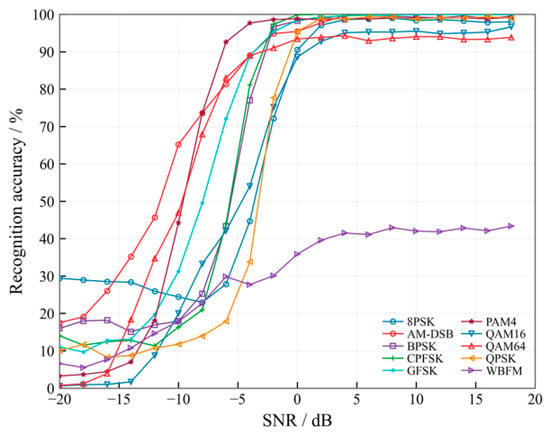
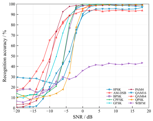
Figure 5 shows the recognition accuracy of ADGNet for different modulation classes on the RadioML2016.10a dataset under different SNR conditions. Overall, the recognition accuracy of most modulation classes increases as the SNR improves and gradually becomes stable in the medium- and high-SNR regions. Three distinct saturation levels can be observed for different modulation classes in the medium- and high-SNR regions. This phenomenon indicates that the modulation categories exhibit different levels of intrinsic separability under the current feature representation. CPFSK, GFSK, and PAM4 reach relatively high saturation accuracies, whereas PSK and high-order QAM signals require higher SNRs before their recognition performance becomes stable. The analog modulation classes, particularly AM-DSB and WBFM, show larger fluctuations and lower saturation levels. These observations suggest that different modulation families have different sensitivities to noise and different feature-separation difficulties. The figure therefore reflects class-dependent recognition characteristics rather than a uniform convergence behavior across all modulation types.

Figure 5. Classification accuracy of each modulation signal type under different SNR conditions.

For high-order modulation signals such as 16QAM and 64QAM, the distance between constellation points is relatively small. As a result, these signals are more sensitive to noise disturbance under low-SNR conditions, and their recognition accuracy increases more slowly. However, as the SNR increases, the recognition performance of these two classes improves significantly, indicating that ADGNet has a certain ability to distinguish fine-grained amplitude–phase features. In contrast, the recognition accuracy of WBFM fluctuates more obviously, suggesting that complex analog modulation signals remain difficult to identify. Overall, Figure 5 shows that ADGNet maintains relatively high recognition accuracy for most digital modulation classes at medium and high SNRs, while high-order QAM and analog modulation classes remain comparatively more challenging.

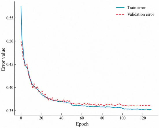
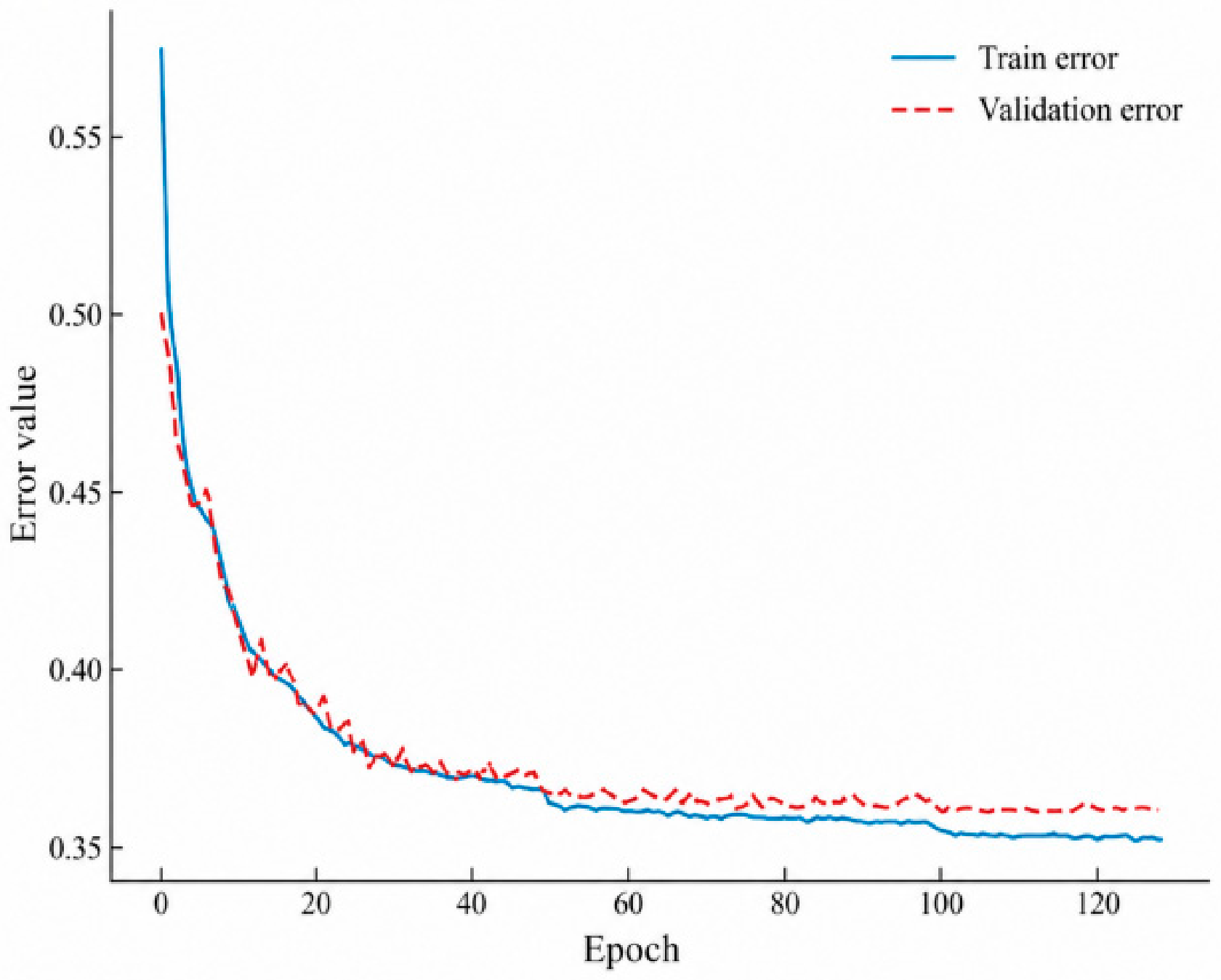
Figure 6 presents the training and validation loss curves of the full ADGNet on the RadioML2016.10b dataset using training seed 1234. As the number of training epochs increases, both losses decrease rapidly during the early training stage and gradually stabilize after approximately 50 epochs. The relatively small gap between the training and validation curves indicates that the optimization process remains stable, with no pronounced divergence between the two curves.

Figure 6. Training and validation loss curves of the full ADGNet on RadioML2016.10b using training seed 1234.

5.1. Comparison with Existing Methods

For a given SNR value $\mathrm{s}$, let the corresponding test subset be denoted by ${\mathcal{D}}_s={\left\{(x_i,y_i)\right\}}_{i=1}^{N_s}$, where $x_i$ is the $i$-th input sample and $y_i$ is its ground-truth modulation label. The recognition accuracy under this SNR is defined as

$$\mathrm{Acc}(s)={\displaystyle \frac{1}{\left|{\mathcal{D}}_s\right|}}{\displaystyle \sum _{(x_i,y_i)\in {\mathcal{D}}_s}\mathbb{I}}\left({\widehat{y}}_i=y_i\right)$$

(25)

where ${\widehat{y}}_i=f(x_i)$ denotes the predicted modulation class, $y_i$ denotes the corresponding ground-truth class, and $\mathbb{I}(\cdot )$ is the indicator function. Specifically, $\mathbb{I}\left({\widehat{y}}_i=y_i\right)=1$ when the prediction is correct; otherwise, it equals 0.

Furthermore, the average accuracy over all SNR values is calculated to evaluate the overall recognition performance:

$$\overline{\mathrm{Acc}}={\displaystyle \frac{1}{\left|\Gamma \right|}}{\displaystyle \sum _{s\in \Gamma }\mathrm{Acc}}(s)$$

(26)

where $\Gamma$ denotes the SNR set in the test data.

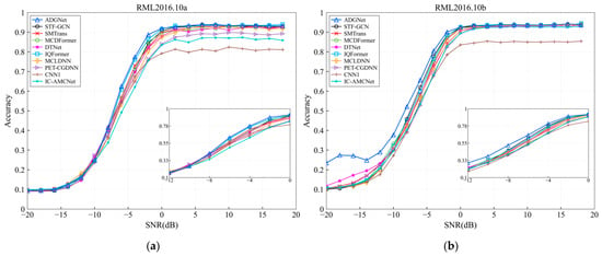
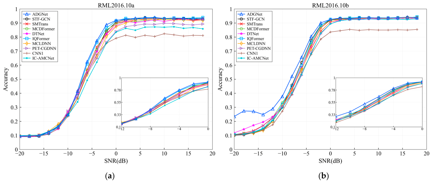
Figure 7 compares the recognition accuracy of different models on RadioML2016.10a and RadioML2016.10b. The proposed ADGNet achieves competitive overall recognition performance on both datasets, with a more pronounced advantage on RadioML2016.10b. As the SNR increases, the accuracy of all models generally improves and gradually becomes stable after 0 dB. ADGNet shows a more obvious advantage in the low-SNR range from −12 dB to 0 dB, especially in the transition range from −8 dB to −4 dB. This result indicates that the proposed model can more effectively extract weak discriminative features under noise interference.

Figure 7. Recognition accuracy of different methods at various SNRs on (a) RadioML2016.10a and (b) RadioML2016.10b.

Compared with convolutional models such as CNN [4] and IC-AMCNet [5], ADGNet not only preserves the ability to extract local waveform features, but also enhances non-stationary local details through the adaptive wavelet front-end. Compared with convolutional recurrent hybrid models such as MCLDNN [6] and PET-CGDNN [7], ADGNet further introduces the dual-domain adaptive encoder to improve complementary representation between the main I/Q features and auxiliary features. Compared with high-performance hybrid models such as SMTrans [10], IQFormer [16], MCDFormer [17] and DTNet [30], ADGNet strengthens relation modeling among temporal nodes through the G2 dynamic topology construction module. Therefore, it shows more stable performance under low-SNR conditions.

Table 3 compares the model size, average recognition accuracy, and batch-amortized inference time of the evaluated methods. For the models reproduced under the same local evaluation pipeline, the reported inference time represents the average processing time per sample obtained with an evaluation batch size of 512. Therefore, these values characterize batch-level throughput efficiency rather than batch-size-one latency. For STF-GCN [19] and CTGNet [20], only the accuracy values reported in the corresponding original publications are included because their complexity and latency were not evaluated under the same experimental environment.

Table 3. Comparison of recognition performance and computational characteristics of different methods.

Model	RadioML2016.10a			RadioML2016.10b
	Parameters	Batch-Amortized Inference Time/$\mathbf{ms}\cdot {\mathbf{sample}}^{-1}$	Average Accuracy/%	Parameters	Batch-Amortized Inference Time/$\mathbf{ms}\cdot {\mathbf{sample}}^{-1}$	Average Accuracy/%
ADGNet	136,434	0.0455	64.23	136,305	0.0282	69.69
CNN1	1,592,383	0.0020	56.03	1,592,126	0.0015	59.09
IC-AMCNet	1,184,459	0.0033	58.35	1,184,202	0.0024	63.34
MCLDNN	406,199	0.0180	61.81	406,070	0.0160	64.20
PET-CGDNN	71,781	0.0095	60.17	71,742	0.0088	63.68
MCDFormer	537,412	0.0938	62.78	537,155	0.0432	65.15
IQFormer	355,049	0.2853	63.80	354,984	0.3632	65.41
DTNet	186,957	0.0117	62.32	186,916	0.0115	65.01
SMTrans	66,316	0.0141	63.02	66,251	0.0111	65.06
STF-GCN	—	—	64.35	—	—	66.04
CTGNet	—	—	62.07	—	—	64.33

Note: The inference times reported for the locally evaluated models are batch-amortized measurements obtained with an evaluation batch size of 512 and should not be interpreted as batch-size-one latency. The accuracy results of STF-GCN and CTGNet are taken from their corresponding original publications; unavailable or non-unified complexity and latency results are denoted by “—”.

ADGNet achieves competitive overall recognition performance on both datasets. On RadioML2016.10a, ADGNet obtains an average accuracy of 64.23%, which is comparable to the 64.35% reported by STF-GCN. On RadioML2016.10b, ADGNet achieves an average accuracy of 69.69%, exceeding the reported accuracies of the other methods listed in Table 3. These results indicate that the performance advantage of ADGNet is more pronounced on RadioML2016.10b rather than being uniformly dominant across both datasets.

In terms of model size, ADGNet contains approximately 0.13 million parameters, which is substantially smaller than CNN1, IC-AMCNet, MCLDNN, MCDFormer, IQFormer, and DTNet. PET-CGDNN and SMTrans employ fewer parameters, but their average recognition accuracies are lower under the reported evaluation settings. The batch-amortized inference results further show that ADGNet maintains moderate computational throughput while improving recognition accuracy. Overall, ADGNet provides a favorable balance between recognition performance and model complexity without relying on a large parameter budget.

Compared with STF-GCN and CTGNet, ADGNet jointly introduces a learnable wavelet-inspired local-detail representation, domain-specific feature recalibration, and sample-specific top-k topology construction within a unified framework.

Although ADGNet requires a higher batch-amortized inference time than CNN1, it improves the average recognition accuracy by 8.20 and 10.60 percentage points on RadioML2016.10a and RadioML2016.10b, respectively, while maintaining a substantially smaller parameter count.

5.2. Low-SNR Performance and Ablation Study

Table 4 reports the detailed recognition results of different models on the RadioML2016.10b dataset under low-SNR conditions from −12 dB to 0 dB. ADGNet achieves recognition accuracies of 27.91%, 37.28%, 50.69%, 65.39%, 80.28%, 89.98% and 92.80% at −12 dB, −10 dB, −8 dB, −6 dB, −4 dB, −2 dB and 0 dB, respectively. Overall, these results are higher than those of the comparison models. This indicates that ADGNet can maintain stronger feature discrimination ability under low-SNR conditions and verifies the effectiveness of adaptive wavelet enhancement, dual-domain feature fusion, and dynamic graph construction.

Table 4. Modulation recognition results of different models on RadioML2016.10b under low-SNR conditions.

Model	Classification Accuracy
	−12 dB	−10 dB	−8 dB	−6 dB	−4 dB	−2 dB	0 dB
ADGNet	27.91	37.28	50.69	65.39	80.28	89.98	92.80
CNN1	17.58	27.23	39.28	55.04	67.71	78.57	83.60
IC-AMCNet	20.63	29.58	40.36	53.38	68.27	82.88	89.45
MCLDNN	19.93	30.79	43.08	56.98	71.40	84.35	90.76
PET-CGDNN	22.29	30.58	38.95	52.77	69.03	82.33	89.49
MCDFormer	22.91	33.32	43.48	57.61	75.18	87.46	92.03
IQFormer	21.10	32.23	44.93	59.75	76.44	88.42	92.66
DTNet	23.19	30.57	43.58	58.40	72.46	84.12	90.74
SMTrans	22.70	30.67	42.02	58.04	74.07	86.63	92.04

To further verify the effectiveness of each core module, ablation experiments are conducted on the RadioML2016.10b dataset. The baseline denotes the basic model without AWN, DDAE, and G2. The variants w/o AWN, w/o DDAE, and w/o G2 denote the models obtained by removing the corresponding module from ADGNet.

As shown in Table 5, the single-module configurations are used to examine the individual effects of AWN, DDAE, and G2, whereas the two-module configurations are used to assess their interactions within the complete architecture. In particular, the comparison between AWN + DDAE and the full ADGNet evaluates the incremental effect of G2 after adaptive wavelet enhancement and dual-domain feature fusion have been introduced. The repeated-run results in Table A5 are further used to assess the stability and statistical significance of these performance differences.

Table 5. Ablation study results.

Model	Parameters	Peak Accuracy/%	Average Accuracy in −12 dB to 0 dB/%	Average Accuracy in −20 dB to 18 dB/%
Baseline	134,656	94.21	59.51	65.32
AWN only	135,680	94.27	60.24	65.97
DDAE only	135,216	94.27	63.04	69.19
G2 only	134,721	94.28	60.07	65.84
w/o AWN	135,281	94.20	58.21	64.94
w/o DDAE	135,745	94.24	58.18	64.91
w/o G2	136,240	94.21	63.13	69.03
ADGNet	136,305	94.24	63.48	69.69

The fact that the w/o AWN and w/o DDAE variants perform below the baseline further indicates that the remaining modules do not contribute independently. Removing one component changes the feature distribution presented to the other modules and may lead to an unfavorable interaction between the remaining feature-fusion and graph-reasoning stages. Therefore, the removal effects should not be interpreted as independent marginal gains.

The peak accuracies of all configurations remain within a narrow range of 94.20–94.28%, indicating that the proposed modules mainly improve robustness in the low-SNR region rather than raising the recognition ceiling under favorable high-SNR conditions.

The ablation results show that the performance changes caused by the three modules are not simply additive. Removing AWN or DDAE from the full architecture results in a clear reduction in low-SNR accuracy, indicating that local-detail enhancement and dual-domain feature recalibration play important roles in the complete model. In comparison, removing G2 changes the overall average accuracy from 69.69% to 69.03%, corresponding to a relatively modest difference. The repeated-run comparison further yields a mean difference of 0.28 percentage points between the full ADGNet and w/o G2, which is not statistically significant at the 0.05 level (p = 0.136). This result suggests that G2 provides only a modest incremental improvement in overall accuracy under the current evaluation protocol. Therefore, G2 is interpreted primarily as an additional mechanism for sample-dependent topology adaptation rather than as the dominant source of the accuracy improvement. Overall, the results suggest that AWN, DDAE, and G2 perform different functional roles in the proposed framework, while their interactions should not be interpreted as simple additive contributions.

5.3. Confusion-Matrix Analysis

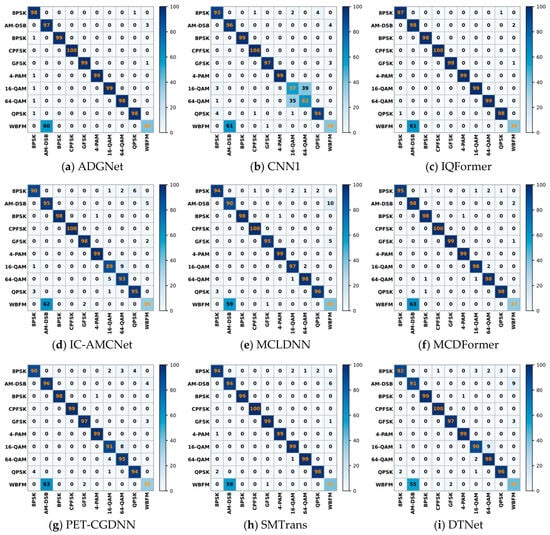
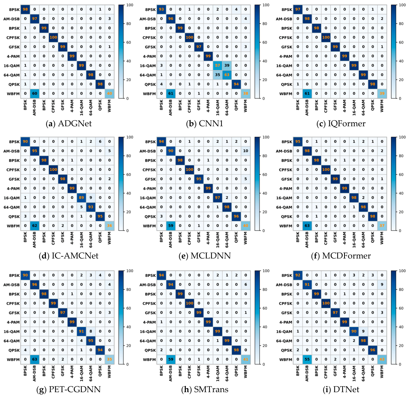
With reference to the analysis of data representations, model structures, and class-confusion phenomena in deep learning-based AMR studies, Figure 8 shows the confusion matrices of different models at 0 dB on the RadioML2016.10b dataset. ADGNet produces higher values on the main diagonal for most digital modulation classes, indicating that its predictions are more concentrated on the ground-truth classes. For BPSK, CPFSK, GFSK, PAM4, and QPSK, the model maintains high recognition accuracy, which shows that the proposed structure can effectively extract key discriminative features from digital modulation signals.

Figure 8. Comparison of confusion matrices for different models at 0 dB.

It is worth noting that 16QAM and 64QAM are easily confused under noisy conditions because of their relatively similar constellation structures. As shown in Figure 8a, ADGNet achieves recognition accuracies of 99% and 98% for 16QAM and 64QAM, respectively, at 0 dB. Similar high class-level accuracies are also observed for several comparison methods. Therefore, these results are interpreted as class-level recognition outcomes rather than being directly attributed to a specific module. Meanwhile, misclassification remains between AM-DSB and WBFM, indicating that analog modulation classes are still more difficult to distinguish under the current feature representation. Overall, the confusion-matrix results show that ADGNet maintains strong recognition performance for most digital modulation classes, while analog-class confusion remains an issue for further investigation.

6. Conclusions

This paper proposes ADGNet, an automatic modulation recognition network integrating adaptive wavelet enhancement and dynamic graph construction, to address the degradation of recognition performance under low-SNR conditions caused by submerged local transient features and blurred modulation class boundaries. The model adopts a dual-branch framework that couples time-domain I/Q features with time–frequency auxiliary features, and leverages a dual-domain adaptive fusion encoder and hierarchical dynamic graph reasoning to jointly extract multi-scale and structural signal characteristics. Experiments on the RadioML2016.10a and RadioML2016.10b datasets verify the competitive performance of ADGNet with a moderate parameter budget. The core contributions of this work are summarized as follows:

• An adaptive wavelet front-end (AWN) is constructed, which replaces fixed wavelet filters with learnable convolution kernels $H_1$, $H_2$ to implement two-level signal decomposition. The data-driven multi-scale high-frequency extraction strategy effectively enhances faint transient modulation features masked by noise and improves feature discrimination at low signal-to-noise ratios.
• A dual-domain adaptive encoder (DDAE) is designed for cross-branch feature recalibration and fusion. Two independent attention branches dynamically adjust the weights of I/Q time-domain features and auxiliary features combining STFT and AWN representations according to sample-dependent feature responses, filtering invalid noise-contaminated features instead of simple feature concatenation.
• A G2 dynamic topology construction module is proposed to introduce sample-dependent graph adaptation. A globally shared learnable coefficient integrates the original rule-based adjacency with a sample-specific dynamic adjacency matrix constructed from the temporal node features of each input signal. Hierarchical graph pooling and graph attention are subsequently employed to extract compact structural representations for modulation classification.

Ablation experiments indicate that AWN and DDAE account for most of the observed improvement in low-SNR recognition, whereas G2 provides an additional mechanism for sample-dependent topology adaptation with a comparatively smaller incremental accuracy gain. ADGNet achieves average recognition accuracies of 64.23% and 69.69% on RadioML2016.10a and RadioML2016.10b, respectively. On RadioML2016.10b, the average accuracy over the −12 to 0 dB range increases from 59.51% for the baseline to 63.48% for ADGNet, corresponding to an improvement of 3.97 percentage points. Over the complete −20 to 18 dB SNR range, the overall average accuracy increases from 65.32% to 69.69%, corresponding to an improvement of 4.37 percentage points. These improvements are achieved with approximately 0.13 million trainable parameters. The confusion-matrix results show that ADGNet maintains high recognition accuracy for most digital modulation classes, while confusion between analog modulation classes remains evident.

This work has several limitations. First, the graph-fusion coefficient is implemented as a globally shared scalar rather than as a sample-dependent weight, which limits the flexibility of graph fusion between the original rule-based adjacency and the learned sample-specific adjacency under rapidly varying noise and channel conditions. Second, the experiments adopt a random sample-level split within each modulation–SNR group. Although this protocol maintains balanced subset distributions, it does not enforce simulation-stream-level or channel-realization-level separation. Related samples may therefore occur across the training, validation, and test subsets, and the reported absolute accuracy may overestimate generalization to independently generated signals. Third, the experiments rely on synthetic RadioML2016 datasets. DeepSig has acknowledged that its early public datasets contain known errata, and the complete generation protocol of RadioML2016.10b is not publicly documented. These issues limit strict reproducibility and prevent the current results from directly representing performance on real over-the-air signals. Finally, although ADGNet maintains a relatively small parameter count, its batch-amortized inference time is higher than that of extremely lightweight CNN baselines, which indicates that further optimization is still required for resource-constrained deployment.

Future work will investigate sample-dependent graph-fusion weights and more stable topology-learning strategies. We will also generate new signal datasets with explicit source-sequence, channel-realization, and simulation-stream identifiers, enabling group-aware train–validation–test partitioning in which all samples from the same generation group are assigned exclusively to one subset. In addition, independently generated signals and real over-the-air measurements will be introduced to evaluate cross-channel and simulation-to-reality generalization. Lightweight convolution, graph sparsification, and structured pruning will also be explored to further reduce the inference latency and computational overhead of ADGNet.

References

- Tian, X.; Zheng, Q.; Li, B.; Qiao, D.; Yu, K.; Wei, Z.; Li, B.; Jiang, H.; Li, X.; Lin, Y.; et al. A Survey on Deep Learning Enabled Automatic Modulation Classification Methods: Data Representations, Model Structures, and Regularization Techniques. Signal Process. 2026, 242, 110444. [Google Scholar] [CrossRef] [Scilit]
- Wang, X.; Zhao, Y.; Huang, Z. A Survey of Deep Transfer Learning in Automatic Modulation Classification. IEEE Trans. Cogn. Commun. Netw. 2025, 11, 1357–1381. [Google Scholar] [CrossRef] [Scilit]
- Dobre, O.A.; Abdi, A.; Bar-Ness, Y.; Su, W. Survey of Automatic Modulation Classification Techniques: Classical Approaches and New Trends. IET Commun. 2007, 1, 137–156. [Google Scholar] [CrossRef] [Scilit]
- O’Shea, T.J.; Corgan, J.; Clancy, T.C. Convolutional Radio Modulation Recognition Networks. In Engineering Applications of Neural Networks, EANN 2016; Jayne, C., Iliadis, L., Eds.; Communications in Computer and Information Science; Springer: Cham, Switzerland, 2016; Volume 629, pp. 213–226. [Google Scholar]
- Hermawan, A.P.; Ginanjar, R.R.; Kim, D.-S.; Lee, J.-M. CNN-Based Automatic Modulation Classification for Beyond 5G Communications. IEEE Commun. Lett. 2020, 24, 1038–1041. [Google Scholar] [CrossRef] [Scilit]
- Xu, J.; Luo, C.; Parr, G.P.; Luo, Y. A Spatiotemporal Multi-Channel Learning Framework for Automatic Modulation Recognition. IEEE Wirel. Commun. Lett. 2020, 9, 1629–1632. [Google Scholar] [CrossRef] [Scilit]
- Zhang, F.; Luo, C.; Xu, J.; Luo, Y. An Efficient Deep Learning Model for Automatic Modulation Recognition Based on Parameter Estimation and Transformation. IEEE Commun. Lett. 2021, 25, 3287–3290. [Google Scholar] [CrossRef] [Scilit]
- Chen, Y.; Dong, B.; Liu, C.; Xiong, W.; Li, S. Abandon Locality: Frame-Wise Embedding Aided Transformer for Automatic Modulation Recognition. IEEE Commun. Lett. 2023, 27, 327–331. [Google Scholar] [CrossRef] [Scilit]
- Wang, Z.; Zhang, W.; Zhao, Z.; Tang, P.; Zhang, Z. Robust Automatic Modulation Classification via a Lightweight Temporal Hybrid Neural Network. Sensors 2024, 24, 7908. [Google Scholar] [CrossRef] [Scilit]
- Huo, Y.; Wang, C.; Liang, J.; Yue, K.; Li, W. SMTrans: An Efficient Automatic Modulation Recognition Network Based on the Scale-Aware Modulation Transformer. Phys. Commun. 2026, 74, 102966. [Google Scholar] [CrossRef] [Scilit]
- Zhang, J.; Wang, T.; Feng, Z.; Yang, S. Toward the Automatic Modulation Classification With Adaptive Wavelet Network. IEEE Trans. Cogn. Commun. Netw. 2023, 9, 549–563. [Google Scholar] [CrossRef] [Scilit]
- Quan, Y.; Cheng, N.; Wang, X.; Yin, Z.; Xu, W.; Wang, D. ALWNN: Automatic Modulation Classification via Adaptive Lightweight Wavelet Neural Network. In Proceedings of the IEEE Global Communications Conference (GLOBECOM 2024), Cape Town, South Africa, 8–12 December 2024; pp. 3835–3840. [Google Scholar]
- Wu, M.; Zou, Z.; Zhang, W.; Liu, G.; Zou, J. Automatic Modulation Classification Based on Wavelet Analysis and Convolution Neural Network. Electronics 2025, 14, 3801. [Google Scholar] [CrossRef] [Scilit]
- Faysal, A.; Boushine, T.; Rostami, M.; Roshan, R.G.; Wang, H.; Muralidhar, N.; Sahoo, A.; Yao, Y.-D. DenoMAE: A Multimodal Autoencoder for Denoising Modulation Signals. IEEE Commun. Lett. 2025, 29, 1659–1663. [Google Scholar] [CrossRef] [Scilit]
- Hou, S.; Dong, Y.; Li, Y.; Yan, Q.; Wang, M.; Fang, S. Multi-Domain-Fusion Deep Learning for Automatic Modulation Recognition in Spatial Cognitive Radio. Sci. Rep. 2023, 13, 10736. [Google Scholar] [CrossRef] [Scilit]
- Shao, M.; Li, D.; Hong, S.; Qi, J.; Sun, H. IQFormer: A Novel Transformer-Based Model with Multi-Modality Fusion for Automatic Modulation Recognition. IEEE Trans. Cogn. Commun. Netw. 2025, 11, 1623–1634. [Google Scholar] [CrossRef] [Scilit]
- Chen, Z.; Zhang, X.; He, K. Multi-Channel Convolutional Distilled Transformer for Automatic Modulation Classification. In Proceedings of the 2024 International Joint Conference on Neural Networks (IJCNN), Yokohama, Japan, 30 June–5 July 2024; pp. 1–8. [Google Scholar]
- Xuan, Q.; Zhou, J.; Qiu, K.; Chen, Z.; Xu, D.; Zheng, S.; Yang, X. AvgNet: Adaptive Visibility Graph Neural Network and Its Application in Modulation Classification. IEEE Trans. Netw. Sci. Eng. 2022, 9, 1516–1526. [Google Scholar] [CrossRef] [Scilit]
- Shao, M.; Fu, Z.; Li, D.; Zhang, F.; Cai, Y.; Hong, S.; Cao, L.; Peng, Y.; Qi, J. STF-GCN: A Multi-Domain Graph Convolution Network Method for Automatic Modulation Recognition via Adaptive Correlation. IEEE Trans. Cogn. Commun. Netw. 2026, 12, 2036–2050. [Google Scholar] [CrossRef] [Scilit]
- Wang, D.; Lin, M.; Zhang, X.; Huang, Y.; Zhu, Y. Automatic Modulation Classification Based on CNN-Transformer Graph Neural Network. Sensors 2023, 23, 7281. [Google Scholar] [CrossRef] [Scilit]
- Liu, X.; Mao, Z.; Liu, M.; Wang, C.; Cai, Z. Automatic Modulation Classification Based on a Dynamic Graph Architecture. Appl. Sci. 2025, 15, 11782. [Google Scholar] [CrossRef] [Scilit]
- Wu, Z.; Pan, S.; Long, G.; Jiang, J.; Zhang, C. Graph WaveNet for Deep Spatial-Temporal Graph Modeling. In Proceedings of the Twenty-Eighth International Joint Conference on Artificial Intelligence, Macao, China, 10–16 August 2019; pp. 1907–1913. [Google Scholar]
- Wu, Z.; Pan, S.; Long, G.; Jiang, J.; Chang, X.; Zhang, C. Connecting the Dots: Multivariate Time Series Forecasting with Graph Neural Networks. In Proceedings of the 26th ACM SIGKDD International Conference on Knowledge Discovery & Data Mining, Virtual Event, 23–27 August 2020; pp. 753–763. [Google Scholar]
- Qi, P.; Zhou, X.; Zheng, S.; Li, Z. Automatic Modulation Classification Based on Deep Residual Networks with Multimodal Information. IEEE Trans. Cogn. Commun. Netw. 2021, 7, 21–33. [Google Scholar] [CrossRef] [Scilit]
- Hu, J.; Shen, L.; Sun, G. Squeeze-and-Excitation Networks. In Proceedings of the IEEE/CVF Conference on Computer Vision and Pattern Recognition (CVPR), Salt Lake City, UT, USA, 18–22 June 2018; pp. 7132–7141. [Google Scholar]
- Kipf, T.N.; Welling, M. Semi-Supervised Classification with Graph Convolutional Networks. In Proceedings of the 5th International Conference on Learning Representations (ICLR), Toulon, France, 24–26 April 2017. [Google Scholar]
- Ying, Z.; You, J.; Morris, C.; Ren, X.; Hamilton, W.L.; Leskovec, J. Hierarchical Graph Representation Learning with Differentiable Pooling. In Advances in Neural Information Processing Systems 31; Bengio, S., Wallach, H., Larochelle, H., Grauman, K., Cesa-Bianchi, N., Garnett, R., Eds.; Curran Associates, Inc.: Red Hook, NY, USA, 2018; pp. 4800–4810. [Google Scholar]
- Veličković, P.; Cucurull, G.; Casanova, A.; Romero, A.; Liò, P.; Bengio, Y. Graph Attention Networks. In Proceedings of the 6th International Conference on Learning Representations (ICLR), Vancouver, BC, Canada, 30 April–3 May 2018. [Google Scholar]
- O’Shea, T.J.; West, N. Radio Machine Learning Dataset Generation with GNU Radio. In Proceedings of the 6th GNU Radio Conference, Knoxville, TN, USA, 16–20 September 2016; Volume 1. [Google Scholar]
- Dao, T.-T.; Pham, Q.-V.; Huynh-The, T.; Hwang, W.-J. Transformer Model Embedding Dual Stream for Modulation Classification of Short Signal Samples. ACM Trans. Intell. Syst. Technol. 2026, 17, 65. [Google Scholar] [CrossRef] [Scilit]
Disclaimer/Publisher’s Note: The statements, opinions and data contained in all publications are solely those of the individual author(s) and contributor(s) and not of MDPI and/or the editor(s). MDPI and/or the editor(s) disclaim responsibility for any injury to people or property resulting from any ideas, methods, instructions or products referred to in the content. |
© 2026 by the authors. Licensee MDPI, Basel, Switzerland. This article is an open access article distributed under the terms and conditions of the Creative Commons Attribution (CC BY) license.