Critical Evaluation of Weighted Similarity Measures and Algorithmic Solutions in Fuzzy Pattern Recognition

Abstract

This study re-examines several published weighted similarity measures for intuitionistic fuzzy pattern recognition problems. This study constructs four counterexamples, each involving two candidate patterns and one sample, to test whether the measure can consistently produce a unique classification decision. The examples show that distinct patterns can receive identical similarity scores under the published formulation; therefore, the measure does not always resolve class assignment in the cases considered here. We then analyze why weighting alone does not necessarily eliminate this difficulty and discuss multi-measure algorithmic alternatives for selected discrete cases. The contribution of this study is, therefore, a counterexample-based critique of the discriminative limitations of weighted similarity measures.

1. Introduction

For two candidate patterns, $A_1$ and $A_2$, and a sample labeled $B$, a pattern recognition task is used to determine to which pattern the sample should be assigned.

Solutions of such problems rely on a similarity measure, denoted as $Sim$, that allows researchers to compute two similarity measures: $Sim\left(A_1,B\right)$ and $Sim\left(A_2,B\right)$. If $Sim\left(A_1,B\right)>Sim\left(A_2,B\right)$, then sample $B$ will be classified as belonging to pattern $A_1$. We express the above idea in the following formal rule.

A well-defined similarity measure should have the following property:

$$Sim\left(A_1,B\right)\ne Sim\left(A_2,B\right),$$

(1)

Then, if

$$Sim\left(A_1,B\right)>Sim\left(A_2,B\right),$$

(2)

sample $B$ will be classified as pattern $A_1$.

On the other hand, if

$$Sim\left(A_1,B\right)<Sim\left(A_2,B\right),$$

(3)

then sample $B$ will be classified as pattern $A_2$. Hence, decision makers can choose the assigned pattern for the examined sample.

Recently, Arefi and Taheri [1] developed several weighted similarity measures, asserting that their measures can help researchers solve pattern recognition problems. In this study, we construct four examples using their measures and identify critical issues that arise in pattern recognition problems; specifically, the four examples serve as counterexamples demonstrating the limitations of the proposed measures.

To date, Arefi and Taheri [1] have been cited eighteen times. We classify these citations into the following three categories:

(a) To derive application-oriented regressions: Arefi [2], Arefi [3,4], and Khammar et al. [5].

(b) To construct new models: Imran et al. [6], Hosseinzadeh et al. [7], Kacprzyk et al. [8], Eslaminasab and Hamzehee [9], and Arefi and Khammar [10].

(c) To develop new similarity measures: Mohamed et al. [11], Rezaei and Rezaei [12,13], Torres-Manzanera et al. [14], Diaz-Vazquez et al. [15], Tiwari [16], Zhao et al. [17], and Huidobro et al. [18].

Among the above citations, none provides a detailed examination of the weighted similarity measures proposed by Arefi and Taheri [1] that were intended to solve the problem of pattern recognition classification. This study tests the robustness of their claims by constructing counterexamples. The contribution does not result in the production of a new classifier but instead serves as a critique of the published method’s discriminative limits.

Recent advances in fuzzy optimization have demonstrated that robust similarity measures for Atanassov’s intuitionistic fuzzy sets are pivotal for high-precision diagnostic systems, as illustrated by Patel et al. [19] in multimodal medical image fusion. The intersection of fuzzy decision algorithms and deep learning has paved the way for advanced pattern recognition paradigms, such as the intelligent visual speech recognition model developed by El Ogri et al. [20], which leverages optimized quaternion moments. Beyond classical intuitionistic frameworks, generalizing similarity measures to higher-order fuzzy representations, such as the distance formulations for Pythagorean fuzzy sets discussed by Ejegwa [21], has emerged as a significant theoretical frontier. Similarly, the modeling capacity of q-rung orthopair fuzzy sets, as investigated by Wang et al. [22], provides a broader mathematical space to mitigate discrimination uncertainty in complex environments. In high-dimensional signal processing, machine learning-driven representations, such as the dual Hahn polynomial framework proposed by El Ogri et al. [23], rely heavily on robust distance metrics to maintain classification integrity during compression. Moreover, optimizing parameter weights remains a fundamental challenge in computational models; here, the generalized Laguerre polynomial optimization methodology developed by Bousraraf et al. [24] offers a rigorous regression paradigm that can be effectively mapped to weight-tuning in fuzzy decision systems. This paradigm is further exemplified in 3D image recognition, where El Ogri et al. [25] employed fractional-order Legendre moments coupled with deep neural networks, demonstrating the critical role of exact mathematical expressions in reducing error propagation.

This study is organized as follows. Section 2 introduces notation. Section 3 reviews the published measure. Section 4 explains the motivating intuition. Section 5, Section 6, Section 7 and Section 8 present the counterexamples. Section 9 analyzes the weighting issue. Section 10 illustrates an alternative algorithm. Section 11 discusses the strengths and advantages of the proposed analysis. Section 12 concludes this study.

2. Nomenclature

For two candidate patterns, $A_1$ and $A_2$, and a sample $B$, the pattern recognition task is to determine to which pattern the sample should be assigned.

$X$ is the universe of discourse. For the discrete case, $X=\left\{x_1,x_2,\dots ,x_n\right\}$.

${\mu }_{\tilde{A}}\left(x_i\right)$ is the membership function at $x_i$.

$v_{\tilde{A}}\left(x_i\right)$ is the non-membership function at $x_i$.

$\left[{\mu }_{\tilde{A}}\left(x_i\right),1-v_{\tilde{A}}\left(x_i\right)\right]$ is the expression proposed by Arefi and Taheri [1].

$\tilde{A}$ is an intuitionistic fuzzy set, with $\tilde{A}=\left\{\left(x_i,\left[{\mu }_{\tilde{A}}\left(x_i\right),1-v_{\tilde{A}}\left(x_i\right)\right]\right):i=\mathrm{1,2},\dots ,n\right\}$.

$Sim\left( , \right)$ is an abbreviation for a similarity measure.

$S{T}_{\mu }\left(\tilde{A},\tilde{B}\right)$ is an abbreviation proposed by Arefi and Taheri [1], with $S{T}_{\mu }\left(\tilde{A},\tilde{B}\right)={\sum }_{i=1}^n\left({\mu }_{\tilde{A}}\left(x_i\right)+{\mu }_{\tilde{B}}\left(x_i\right)\right)$.

$S{T}_v\left(\tilde{A},\tilde{B}\right)$ is an abbreviation proposed by Arefi and Taheri [1], with $S{T}_v\left(\tilde{A},\tilde{B}\right)={\sum }_{i=1}^n\left(1-v_{\tilde{A}}\left(x_i\right)+1-v_{\tilde{B}}\left(x_i\right)\right)$.

$S_w\left(\tilde{A},\tilde{B}\right)$ is the similarity measure for two intuitionistic fuzzy sets, $\tilde{A}$ and $\tilde{B}$, proposed by Arefi and Taheri [1].

${\mu }_{\tilde{B}}\left(x_i\right)$ is defined by this study to stand for the midpoint of ${\mu }_{{\tilde{A}}_1}\left(x_i\right)$ and ${\mu }_{{\tilde{A}}_2}\left(x_i\right)$, with ${\mu }_{\tilde{B}}\left(x_i\right)=\left[{\mu }_{{\tilde{A}}_1}\left(x_i\right)+{\mu }_{{\tilde{A}}_2}\left(x_i\right)\right]/2$.

$v_{\tilde{B}}\left(x_i\right)$ is defined by this study to stand for the midpoint of $v_{{\tilde{A}}_1}\left(x_i\right)$ and $v_{{\tilde{A}}_2}\left(x_i\right)$, with $v_{\tilde{B}}\left(x_i\right)=\left[v_{{\tilde{A}}_1}\left(x_i\right)+v_{{\tilde{A}}_2}\left(x_i\right)\right]/2$.

$dist\left(\alpha ,\beta \right)$ is the distance between $\alpha$ and $\beta$, proposed by Chou [26].

$S_D\left( , \right)$ is the similarity measure proposed by Deng et al. [27].

${\mathrm{S}}_{\mathrm{p},\lambda ,\mathrm{w}}\left( , \right)$ is the first similarity measure proposed by Yen et al. [28].

${\mathrm{S}}_{\mathrm{p},\lambda ,\mathrm{w},\mathrm{M}}\left( , \right)$ is the second similarity measure proposed by Yen et al. [28].

${\mu }_1$ is the differential divergence parameters for the membership function between ${\tilde{A}}_1$ and $\tilde{B}$, with ${\mu }_1={\displaystyle \frac{{\sum }_{i=1}^4\left|{\mu }_{{\tilde{A}}_1}\left(x_i\right)-{\mu }_{\tilde{B}}\left(x_i\right)\right|}{S{T}_{\mu }\left({\tilde{A}}_1,\tilde{B}\right)}}$.

${\mu }_2$ is the differential divergence parameters for the membership function between ${\tilde{A}}_2$ and $\tilde{B}$, with ${\mu }_2={\displaystyle \frac{{\sum }_{i=1}^4\left|{\mu }_{{\tilde{A}}_2}\left(x_i\right)-{\mu }_{\tilde{B}}\left(x_i\right)\right|}{S{T}_{\mu }\left({\tilde{A}}_2,\tilde{B}\right)}}$.

$v_1$ is the differential divergence parameters for the non-membership function between ${\tilde{A}}_1$ and $\tilde{B}$, with $v_1={\displaystyle \frac{{\sum }_{i=1}^4\left|v_{{\tilde{A}}_1}\left(x_i\right)-v_{\tilde{B}}\left(x_i\right)\right|}{S{T}_v\left({\tilde{A}}_1,\tilde{B}\right)}}$.

$v_2$ is the differential divergence parameters for the non-membership function between ${\tilde{A}}_2$ and $\tilde{B}$, with $v_2={\displaystyle \frac{{\sum }_{i=1}^4\left|{\mu }_{{\tilde{A}}_2}\left(x_i\right)-{\mu }_{\tilde{B}}\left(x_i\right)\right|}{S{T}_{\mu }\left({\tilde{A}}_2,\tilde{B}\right)}}$.

${∆}_{\mu }$ is the differential divergence parameters for the membership function, among ${\tilde{A}}_1$, ${\tilde{A}}_2$ and $\tilde{B}$, with ${∆}_{\mu }={\mu }_1-{\mu }_2$.

${∆}_v$ is a new abbreviation, the differential divergence parameters for the non-membership function, among ${\tilde{A}}_1$, ${\tilde{A}}_2$ and $\tilde{B}$, with ${∆}_v =v_1-v_2$.

$∆$ is the joint differential divergence parameter, with $∆={∆}_{\mu }{∆}_v$.

3. Background

Arefi and Taheri [1] reviewed several earlier similarity measures, including those of Li and Cheng [29], Liang and Shi [30], Zeng and Guo [31], Farhadinia [32], and Wang and Xin [33], and argued that these measures may fail to resolve some pattern recognition tasks, with two patterns ${\tilde{P}}_1$ and ${\tilde{P}}_2$, and a sample $\tilde{S}$, using a given similarity measure, denoted as $Sim$, when

$$Sim\left({\tilde{P}}_1,\tilde{S}\right)=Sim\left({\tilde{P}}_2,\tilde{S}\right).$$

(4)

The undecided dilemma occurs for Li and Cheng [29], Liang and Shi [30], Zeng and Guo [31], Farhadinia [32] and Wang and Xin [33]. Consequently, Arefi and Taheri [1] constructed their similarity measure, $S_w$, under discrete and continuous scenarios as follows.

Under the discrete scenario, Arefi and Taheri [1], let $X=\left\{x_1,x_2,\dots ,x_n\right\}$ be the universe of discourse for two intuitionistic fuzzy sets, $\tilde{A}$ and $\tilde{B}$, with

$$\tilde{A}=\left\{\left(x_i,\left[{\mu }_{\tilde{A}}\left(x_i\right),1-v_{\tilde{A}}\left(x_i\right)\right]\right):i=\mathrm{1,2},\dots ,n\right\},$$

(5)

and

$$\tilde{B}=\left\{\left(x_i,\left[{\mu }_{\tilde{B}}\left(x_i\right),1-v_{\tilde{B}}\left(x_i\right)\right]\right):i=\mathrm{1,2},\dots ,n\right\}.$$

(6)

The sum of lower bounds between $\tilde{A}$ and $\tilde{B}$, denoted as $S{T}_{\mu }\left(\tilde{A},\tilde{B}\right)$ is

$$S{T}_{\mu }\left(\tilde{A},\tilde{B}\right)={\sum }_{i=1}^n\left({\mu }_{\tilde{A}}\left(x_i\right)+{\mu }_{\tilde{B}}\left(x_i\right)\right).$$

(7)

The sum of upper bounds between $\tilde{A}$ and $\tilde{B}$, denoted as $S{T}_v\left(\tilde{A},\tilde{B}\right)$ is

$$S{T}_v\left(\tilde{A},\tilde{B}\right)={\sum }_{i=1}^n\left(1-v_{\tilde{A}}\left(x_i\right)+1-v_{\tilde{B}}\left(x_i\right)\right).$$

(8)

The weighted similarity measure is defined as

$$S_w\left(\tilde{A},\tilde{B}\right)=1-w{\displaystyle \frac{{\sum }_{i=1}^n\left|{\mu }_{\tilde{A}}\left(x_i\right)-{\mu }_{\tilde{B}}\left(x_i\right)\right|}{S{T}_{\mu }\left(\tilde{A},\tilde{B}\right)}}-\left(1-w\right){\displaystyle \frac{{\sum }_{i=1}^n\left|v_{\tilde{A}}\left(x_i\right)-v_{\tilde{B}}\left(x_i\right)\right|}{S{T}_v\left(\tilde{A},\tilde{B}\right)}}.$$

(9)

Under the continuous scenario, Arefi and Taheri [1] defined that

$$S_w\left(\tilde{A},\tilde{B}\right)=1-w{\displaystyle \frac{{\int }_{-\infty }^{\infty }\left|{\mu }_{\tilde{A}}\left(x\right)-{\mu }_{\tilde{B}}\left(x\right)\right|dx}{{\int }_{-\infty }^{\infty }{\mu }_{\tilde{A}}\left(x\right)dx+{\int }_{-\infty }^{\infty }{\mu }_{\tilde{B}}\left(x\right)dx}}-\left(1-w\right){\displaystyle \frac{{\int }_{-\infty }^{\infty }\left|v_{\tilde{A}}\left(x\right)-v_{\tilde{B}}\left(x\right)\right|dx}{{\int }_{-\infty }^{\infty }{v}_{\tilde{A}}\left(x\right)dx+{\int }_{-\infty }^{\infty }{v}_{\tilde{B}}\left(x\right)dx}}.$$

(10)

In Section 4, Section 5, Section 6, Section 7 and Section 8, we discuss the midpoint property.

In Section 7, Lemmas 1 and 2, we discuss the midpoint property. Arefi and Taheri [1] tried to avoid the midpoint problem, and then Arefi and Taheri [1] constructed their new similarity measure under non-Euclidean distance. Based on Theorem 3, we found conditions to result in a pattern recognition dilemma, under non-Euclidean distance environments. In Section 10, we developed two novel similarity measures, which will provide the motivation for the similarity measure proposed by Arefi and Taheri [1].

4. The Simplest Case Motivating Our First Counterexample

We begin with an illustrative case on the simplest universe of discourse, $X=\left\{x_1,x_3\right\}$, to assume that

$${\tilde{A}}_1=\left\{\left(x_1,\left[\mathrm{0.2,0.8}\right]\right),\left(x_3,\left[\mathrm{0.3,0.7}\right]\right)\right\},$$

(11)

$${\tilde{A}}_2=\left\{\left(x_1,\left[\mathrm{0.3,0.7}\right]\right),\left(x_3,\left[\mathrm{0.2,0.8}\right]\right)\right\},$$

(12)

and

$$\tilde{B}=\left\{\left(x_1,\left[a,b\right]\right),\left(x_3,\left[a,b\right]\right)\right\}.$$

(13)

Thus, the two intuitionistic fuzzy sets, ${\tilde{A}}_1$ and ${\tilde{A}}_2$, can be treated as a shift between $x_1$ and $x_3$, and $\tilde{B}$ is duplication for $x_1$ and $x_3$. Hence, we know

$$\begin{gathered} {\mu }_{{\tilde{A}}_1}\left(x_1\right)={\mu }_{{\tilde{A}}_2}\left(x_3\right),v_{{\tilde{A}}_1}\left(x_1\right)=v_{{\tilde{A}}_2}\left(x_3\right),{\mu }_{{\tilde{A}}_1}\left(x_3\right)={\mu }_{{\tilde{A}}_2}\left(x_1\right),v_{{\tilde{A}}_1}\left(x_3\right)=v_{{\tilde{A}}_2}\left(x_1\right), \\ {\mu }_{\tilde{B}}\left(x_1\right)={\mu }_{\tilde{B}}\left(x_3\right),\mathrm{and} v_{\tilde{B}}\left(x_1\right)=v_{\tilde{B}}\left(x_3\right). \end{gathered}$$

(14)

Based on Equation (14), we derive

$$\begin{gathered} S{T}_{\mu }\left({\tilde{A}}_1,\tilde{B}\right)={\mu }_{{\tilde{A}}_1}\left(x_1\right)+{\mu }_{\tilde{B}}\left(x_1\right)+{\mu }_{{\tilde{A}}_1}\left(x_3\right)+{\mu }_{\tilde{B}}\left(x_3\right), \\ ={\mu }_{{\tilde{A}}_2}\left(x_3\right)+{\mu }_{\tilde{B}}\left(x_3\right)+{\mu }_{{\tilde{A}}_2}\left(x_1\right)+{\mu }_{\tilde{B}}\left(x_1\right), \\ =S{T}_{\mu }\left({\tilde{A}}_2,\tilde{B}\right), \end{gathered}$$

(15)

and

$$\begin{gathered} S{T}_v\left({\tilde{A}}_1,\tilde{B}\right)=\left[1-v_{{\tilde{A}}_1}\left(x_1\right)\right]+\left[1-v_{\tilde{B}}\left(x_1\right)\right]+\left[1-v_{{\tilde{A}}_1}\left(x_3\right)\right]+\left[1-v_{\tilde{B}}\left(x_3\right)\right], \\ =\left[1-v_{{\tilde{A}}_2}\left(x_3\right)\right]+\left[1-v_{\tilde{B}}\left(x_3\right)\right]+\left[1-v_{{\tilde{A}}_2}\left(x_1\right)\right]+\left[1-v_{\tilde{B}}\left(x_1\right)\right], \\ =S{T}_v\left({\tilde{A}}_2,\tilde{B}\right). \end{gathered}$$

(16)

Moreover, we evaluate

$$\begin{gathered} {\sum }_{i=\mathrm{1,3}}\left|{\mu }_{{\tilde{A}}_1}\left(x_i\right)-{\mu }_{\tilde{B}}\left(x_i\right)\right|=\left|{\mu }_{{\tilde{A}}_1}\left(x_1\right)-{\mu }_{\tilde{B}}\left(x_1\right)\right|+\left|{\mu }_{{\tilde{A}}_1}\left(x_3\right)-{\mu }_{\tilde{B}}\left(x_3\right)\right|, \\ =\left|{\mu }_{{\tilde{A}}_2}\left(x_3\right)-{\mu }_{\tilde{B}}\left(x_3\right)\right|+\left|{\mu }_{{\tilde{A}}_2}\left(x_1\right)-{\mu }_{\tilde{B}}\left(x_1\right)\right|, \\ ={\sum }_{i=\mathrm{1,3}}\left|{\mu }_{{\tilde{A}}_2}\left(x_i\right)-{\mu }_{\tilde{B}}\left(x_i\right)\right|, \end{gathered}$$

(17)

and

$$\begin{gathered} {\sum }_{i=\mathrm{1,3}}\left|v_{{\tilde{A}}_1}\left(x_i\right)-v_{\tilde{B}}\left(x_i\right)\right|=\left|v_{{\tilde{A}}_1}\left(x_1\right)-v_{\tilde{B}}\left(x_1\right)\right|+\left|v_{{\tilde{A}}_1}\left(x_3\right)-v_{\tilde{B}}\left(x_3\right)\right|, \\ =\left|v_{{\tilde{A}}_2}\left(x_3\right)-v_{\tilde{B}}\left(x_3\right)\right|+\left|v_{{\tilde{A}}_2}\left(x_1\right)-v_{\tilde{B}}\left(x_1\right)\right|, \\ ={\sum }_{i=\mathrm{1,3}}\left|v_{{\tilde{A}}_2}\left(x_i\right)-v_{\tilde{B}}\left(x_i\right)\right|. \end{gathered}$$

(18)

Based on Equations (15) and (17), we obtain

$${\displaystyle \frac{{\sum }_{i=\mathrm{1,3}}\left|{\mu }_{{\tilde{A}}_1}\left(x_i\right)-{\mu }_{\tilde{B}}\left(x_i\right)\right|}{S{T}_{\mu }\left({\tilde{A}}_1,\tilde{B}\right)}}={\displaystyle \frac{{\sum }_{i=\mathrm{1,3}}\left|{\mu }_{{\tilde{A}}_2}\left(x_i\right)-{\mu }_{\tilde{B}}\left(x_i\right)\right|}{S{T}_{\mu }\left({\tilde{A}}_2,\tilde{B}\right)}},$$

(19)

and based on Equations (16) and (18), we find

$${\displaystyle \frac{{\sum }_{i=\mathrm{1,3}}\left|v_{{\tilde{A}}_1}\left(x_i\right)-v_{\tilde{B}}\left(x_i\right)\right|}{S{T}_v\left({\tilde{A}}_1,\tilde{B}\right)}}={\displaystyle \frac{{\sum }_{i=\mathrm{1,3}}\left|v_{{\tilde{A}}_2}\left(x_i\right)-v_{\tilde{B}}\left(x_i\right)\right|}{S{T}_v\left({\tilde{A}}_2,\tilde{B}\right)}}.$$

(20)

From the above discussion, we extend the universe of discourse from $X=\left\{x_1,x_3\right\}$ to $X=\left\{x_1,x_2,x_3,x_4\right\}$ under the same argument as

$$\begin{gathered} {\mu }_{{\tilde{A}}_1}\left(x_2\right)={\mu }_{{\tilde{A}}_2}\left(x_4\right),v_{{\tilde{A}}_1}\left(x_2\right)=v_{{\tilde{A}}_2}\left(x_4\right),{\mu }_{{\tilde{A}}_1}\left(x_4\right)={\mu }_{{\tilde{A}}_2}\left(x_2\right),v_{{\tilde{A}}_1}\left(x_4\right)=v_{{\tilde{A}}_2}\left(x_2\right), \\ {\mu }_{\tilde{B}}\left(x_2\right)={\mu }_{\tilde{B}}\left(x_4\right),\mathrm{and} v_{\tilde{B}}\left(x_2\right)=v_{\tilde{B}}\left(x_4\right). \end{gathered}$$

(21)

Therefore, we obtain

$$S{T}_{\mu }\left({\tilde{A}}_1,\tilde{B}\right)=S{T}_{\mu }\left({\tilde{A}}_2,\tilde{B}\right),$$

(22)

and

$$S{T}_v\left({\tilde{A}}_1,\tilde{B}\right)=S{T}_v\left({\tilde{A}}_2,\tilde{B}\right).$$

(23)

Moreover, we also imply

$${\sum }_{i=1}^4\left|{\mu }_{{\tilde{A}}_1}\left(x_i\right)-{\mu }_{\tilde{B}}\left(x_i\right)\right|={\sum }_{i=1}^4\left|{\mu }_{{\tilde{A}}_2}\left(x_i\right)-{\mu }_{\tilde{B}}\left(x_i\right)\right|,$$

(24)

and

$${\sum }_{i=1}^4\left|v_{{\tilde{A}}_1}\left(x_i\right)-v_{\tilde{B}}\left(x_i\right)\right|={\sum }_{i=1}^4\left|v_{{\tilde{A}}_2}\left(x_i\right)-v_{\tilde{B}}\left(x_i\right)\right|.$$

(25)

Based on Equations (22) and (24), we find

$${\displaystyle \frac{{\sum }_{i=1}^4\left|{\mu }_{{\tilde{A}}_1}\left(x_i\right)-{\mu }_{\tilde{B}}\left(x_i\right)\right|}{S{T}_{\mu }\left({\tilde{A}}_1,\tilde{B}\right)}}={\displaystyle \frac{{\sum }_{i=1}^4\left|{\mu }_{{\tilde{A}}_2}\left(x_i\right)-{\mu }_{\tilde{B}}\left(x_i\right)\right|}{S{T}_{\mu }\left({\tilde{A}}_2,\tilde{B}\right)}},$$

(26)

and based on Equations (23) and (25), we derive

$${\displaystyle \frac{{\sum }_{i=1}^4\left|v_{{\tilde{A}}_1}\left(x_i\right)-v_{\tilde{B}}\left(x_i\right)\right|}{S{T}_v\left({\tilde{A}}_1,\tilde{B}\right)}}={\displaystyle \frac{{\sum }_{i=1}^4\left|v_{{\tilde{A}}_2}\left(x_i\right)-v_{\tilde{B}}\left(x_i\right)\right|}{S{T}_v\left({\tilde{A}}_2,\tilde{B}\right)}}.$$

(27)

Owing to Equations (26) and (27), we show that

$$S_w\left({\tilde{A}}_1,\tilde{B}\right)=S_w\left({\tilde{A}}_2,\tilde{B}\right),$$

(28)

which is valid for any weight $\mathrm{w}$ with $0\le w\le 1$.

The illustrated case as detailed in this section demonstrates a pattern recognition problem that cannot be solved with the similarity measure proposed by Arefi and Taheri [1].

Based on the above discussion, we develop our Theorem 1 as follows.

Theorem 1.

Let two patterns, ${\tilde{A}}_1$ and ${\tilde{A}}_2$, and a sample, $\tilde{B}$, be intuitionistic fuzzy sets defined over the universe of discourse, $X=\left\{x_1,x_2,\dots ,x_n\right\}$. The weighted similarity measure values satisfy the equivalence relation $S_w\left({\tilde{A}}_1,\tilde{B}\right)=S_w\left({\tilde{A}}_2,\tilde{B}\right)$ if and only if the joint differential divergence parameter is non-positive, as $∆\le 0$.

Proof. 

We assume that

$${∆}_{\mu }={\displaystyle \frac{{\sum }_{i=1}^4\left|{\mu }_{{\tilde{A}}_1}\left(x_i\right)-{\mu }_{\tilde{B}}\left(x_i\right)\right|}{S{T}_{\mu }\left({\tilde{A}}_1,\tilde{B}\right)}}-{\displaystyle \frac{{\sum }_{i=1}^4\left|{\mu }_{{\tilde{A}}_2}\left(x_i\right)-{\mu }_{\tilde{B}}\left(x_i\right)\right|}{S{T}_{\mu }\left({\tilde{A}}_2,\tilde{B}\right)}},$$

(29)

$${∆}_v={\displaystyle \frac{{\sum }_{i=1}^4\left|v_{{\tilde{A}}_1}\left(x_i\right)-v_{\tilde{B}}\left(x_i\right)\right|}{S{T}_v\left({\tilde{A}}_1,\tilde{B}\right)}}-{\displaystyle \frac{{\sum }_{i=1}^4\left|v_{{\tilde{A}}_2}\left(x_i\right)-v_{\tilde{B}}\left(x_i\right)\right|}{S{T}_v\left({\tilde{A}}_2,\tilde{B}\right)}},$$

(30)

and

$$∆={∆}_{\mu }{∆}_v.$$

(31)

We compute that

$$S_w\left({\tilde{A}}_1,\tilde{B}\right)-S_w\left({\tilde{A}}_2,\tilde{B}\right)=-w{∆}_{\mu }-\left(1-w\right){∆}_v.$$

(32)

To establish the necessary and sufficient conditions under which the similarity equivalence holds, the analysis is partitioned into two mutually exclusive and collectively exhaustive cases: $∆=0$, and $∆\ne 0$.

Case 1: The joint parameter satisfies $∆=0$. When $∆=0$, we can further divide into the following three cases: (i) ${∆}_{\mu } =0$, and ${∆}_v =0$, (ii) ${∆}_{\mu } \ne 0$, and ${∆}_v =0$, and (iii) ${∆}_{\mu } =0$, and ${∆}_v \ne 0$.

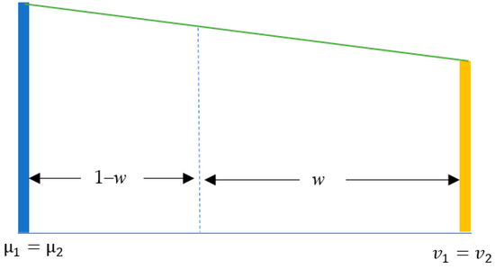
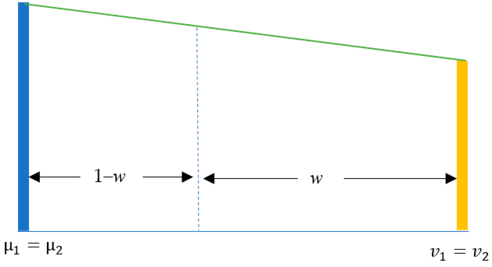
Sub-case (i): Under these symmetrical boundary conditions, substituting the zero parameters (${∆}_{\mu } =0$, and ${∆}_v =0$) into the difference formulation yields: $S_w\left({\tilde{A}}_1,\tilde{B}\right)-\left({\tilde{A}}_2,\tilde{B}\right)=-w\left(0\right)-\left(1-w\right)\left(0\right)$. This equality holds universally for any selection of the relative weight within the closed interval $\left[0,1\right]$. Geometrically, as illustrated in Figure 1, when the individual membership and non-membership distance components are equivalent (${\mu }_1={\mu }_2$ and $v_1=v_2$), any convex combination of these components, represented by $w{\mu }_1+\left(1-w\right)v_1$, will invariably equal $w{\mu }_2+\left(1-w\right)v_2$ under an identical weighting factor $w$. This visual representation confirms that the complement similarity relation ${1-S}_w\left({\tilde{A}}_1,\tilde{B}\right)=1-\left({\tilde{A}}_2,\tilde{B}\right)$ is satisfied, leading to the guaranteed equivalence $S_w\left({\tilde{A}}_1,\tilde{B}\right)=\left({\tilde{A}}_2,\tilde{B}\right)$ for all $w$ in $\left[\mathrm{0,1}\right]$. ${\mu }_1={\mu }_2$ is marked by blue and $v_1=v_2$ is marked by orange. $w{\mu }_1+\left(1-w\right)v_1=w{\mu }_2+\left(1-w\right)v_2$ is marked by green.

Figure 1. ${∆}_{\mu }=0$, and ${∆}_v=0$.

Figure 1 indicates that ${1-S}_w\left({\tilde{A}}_1,\tilde{B}\right)=1-\left({\tilde{A}}_2,\tilde{B}\right)$, such that it follows that $S_w\left({\tilde{A}}_1,\tilde{B}\right)=\left({\tilde{A}}_2,\tilde{B}\right)$ for any selection of $w$.

Sub-case (ii): For this configuration, the selected weight parameter is defined at its boundary value, $w=0$. Substituting this value into the difference formulation yields: $S_w\left({\tilde{A}}_1,\tilde{B}\right)-\left({\tilde{A}}_2,\tilde{B}\right)=-\left(0\right){∆}_{\mu }-\left(1-0\right){∆}_v=0$. Thus, there exists at least one valid parameter boundary ($w=0$) that satisfies the similarity equivalence.

Sub-case (iii): Conversely, defining the weight parameter at its upper boundary, $w=1$, yields: $S_w\left({\tilde{A}}_1,\tilde{B}\right)-\left({\tilde{A}}_2,\tilde{B}\right)=-\left(1\right){∆}_{\mu }-\left(1-1\right){∆}_v=0$. This guarantees the existence of a valid parameter boundary ($w=1$) that satisfies the similarity equivalence.

Consequently, when $∆=0$, a valid weight parameter $w\in \left[\mathrm{0,1}\right]$ always exists to ensure similarity equivalence, which aligns with the condition.

Next, we begin to consider Case 2, the joint parameter satisfying $∆\ne 0$, to find restrictions for $S_w\left({\tilde{A}}_1,\tilde{B}\right)=\left({\tilde{A}}_2,\tilde{B}\right)$.

Under the condition that $∆\ne 0$, the similarity equivalence constraint $S_w\left({\tilde{A}}_1,\tilde{B}\right)=\left({\tilde{A}}_2,\tilde{B}\right)$ requires that $-w{∆}_{\mu }-\left(1-w\right){∆}_v=0$, and then

$$w\left({∆}_v-{∆}_{\mu }\right)={∆}_v.$$

(33)

Since $∆\ne 0$, the boundaries $w=0$ and $w=1$ are mathematically inadmissible, as they would imply ${∆}_v =0$ or ${∆}_{\mu } =0$, respectively, directly violating the non-zero constraint. Therefore, the search for a valid weight is restricted to the open interval $\left(\mathrm{0,1}\right)$. Therefore, in the following, we will consider the selection of $w$, from $0\le w\le 1$ to $0<w<1$.

Motivated by Equation (33), the non-zero joint parameter space, $∆\ne 0$, is partitioned into two sub-cases based on its sign: $\left(\mathsf{\alpha }\right)$ $∆={∆}_{\mu }{∆}_v<0$, and $\left(\mathsf{\beta }\right)$ $∆={∆}_{\mu }{∆}_v>0$.

Sub-case $\left(\mathsf{\alpha }\right)$: This condition implies that the individual differential parameters must possess opposite signs, which is evaluated under two distinct scenarios: $\left(\mathsf{\alpha }1\right)$ ${∆}_{\mu }<0<{∆}_v$ and $\left(\mathsf{\alpha }2\right)$ ${∆}_{\mu } >0>{∆}_v$.

Scenario $\left(\mathsf{\alpha }1\right)$: This algebraic configuration guarantees that the denominator satisfies the inequality ${∆}_v-{∆}_{\mu } >0$. Because ${∆}_v >0$ and ${∆}_v-{∆}_{\mu } >{∆}_v$, the resulting weight ratio is strictly bounded within the open unit interval,

$$0<w={∆}_v/\left({∆}_v-{∆}_{\mu }\right)<1.$$

(34)

Scenario $\left(\mathsf{\alpha }2\right)$: For this configuration, the denominator satisfies ${∆}_v-{∆}_{\mu } <0$. Since both the numerator and the denominator are strictly negative, and the inequality $\left|{∆}_v-{∆}_{\mu }\right|>\left|{∆}_v\right|$ holds, such that the resulting weight ratio remains strictly bounded within the open unit interval,

$$0<w={∆}_v/\left({∆}_v-{∆}_{\mu }\right)<1.$$

(35)

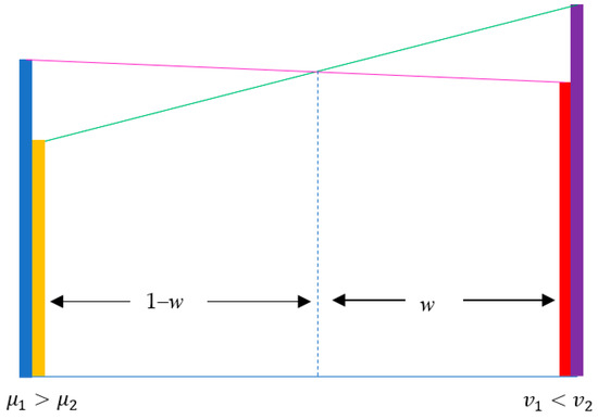
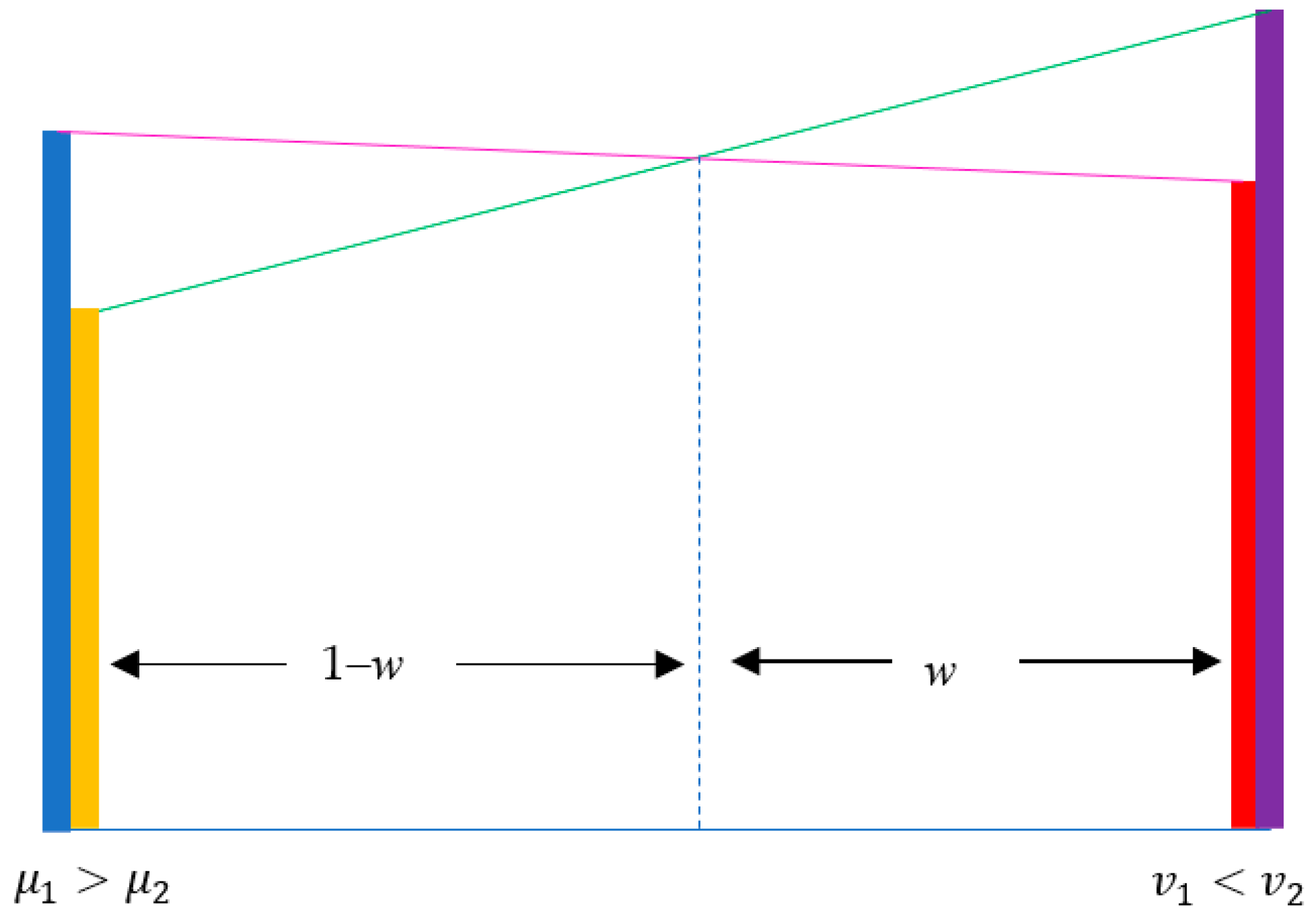
Geometrically, as shown in Figure 2, when ${∆}_{\mu } >0>{∆}_v$ (which implies ${\mu }_1>{\mu }_2$ and $v_1<v_2$), the linear combination curves $\left\{s{\mu }_1+\left(1-s\right)v_1:0<s<1\right\}$ and $\left\{t{\mu }_2+\left(1-t\right)v_2:0<t<1\right\}$ intersect at a unique equilibrium point where the weights satisfy $w={∆}_v/\left({∆}_v-{∆}_{\mu }\right)$ of Equation (35). At this unique intersection, the similarity values are identical, demonstrating that a valid weight always exists when ${∆}_{\mu }>0>{∆}_v$. ${\mu }_1$ is marked by blue, ${\mu }_2$ is marked by orange, $v_1$ is marked by red, and $v_2$ is marked by purple. $w{\mu }_1+\left(1-w\right)v_1$ is marked by pink, and $w{\mu }_2+\left(1-w\right)v_2$ is marked by green.

Figure 2. ${∆}_{\mu }>0>{∆}_v$.

Figure 2 indicates that there is a unique selection of $w$ such that two linear combinations are equal, that is ${1-S}_w\left({\tilde{A}}_1,\tilde{B}\right)=1-\left({\tilde{A}}_2,\tilde{B}\right)$ such that it follows that $S_w\left({\tilde{A}}_1,\tilde{B}\right)=\left({\tilde{A}}_2,\tilde{B}\right)$ for this specific selection of $w$, as $w={∆}_v/\left({∆}_v-{∆}_{\mu }\right)$ of Equation (35).

To date, we prove that if $∆\le 0$, then there exists a proper selection of $w$ such that $S_w\left({\tilde{A}}_1,\tilde{B}\right)=\left({\tilde{A}}_2,\tilde{B}\right)$.

Sub-case $\left(\mathsf{\beta }\right)$: This condition requires that the differential parameters share the same sign, which is analyzed under six exhaustive sub-scenarios: $\left(\mathsf{\beta }1\right)$ ${∆}_v>{∆}_{\mu }>0$, $\left(\mathsf{\beta }2\right)$ ${∆}_v={∆}_{\mu }>0$, $\left(\mathsf{\beta }3\right)$ ${∆}_{\mu }>{∆}_v>0$, $\left(\mathsf{\beta }4\right)$ ${∆}_v <{∆}_{\mu }<0$, $\left(\mathsf{\beta }5\right)$ ${∆}_v ={∆}_{\mu }<0$, $\left(\mathsf{\beta }6\right)$ ${∆}_{\mu }<{∆}_v<0$.

Scenario $\left(\mathsf{\beta }1\right)$: This configuration implies that ${∆}_v-{∆}_{\mu }>0$ and ${∆}_v >{∆}_v-{∆}_{\mu }$, yielding a weight ratio that exceeds unity: ${∆}_v/\left({∆}_v-{∆}_{\mu }\right)>1$.

Scenario $\left(\mathsf{\beta }2\right)$: The denominator collapses to zero (${∆}_v-{∆}_{\mu }=0$), yielding no real mathematical solution for $w$.

Scenario $\left(\mathsf{\beta }3\right)$: Here, the denominator satisfies ${∆}_{\mu }-{∆}_v <0$, which yields a negative weight ratio: ${∆}_v/\left({∆}_v-{∆}_{\mu }\right)<0$.

Scenario $\left(\mathsf{\beta }4\right)$: This configuration implies that ${∆}_v-{∆}_{\mu }<0$ and $\left|{∆}_v-{∆}_{\mu }\right|<\left|{∆}_v\right|$. Because both terms are negative, the ratio exceeds unity: ${∆}_v/\left({∆}_v-{∆}_{\mu }\right)>1$.

Scenario $\left(\mathsf{\beta }5\right)$: This leads to a zero denominator (${∆}_v-{∆}_{\mu } =0$), meaning no real mathematical solution exists for $w$.

Scenario $\left(\mathsf{\beta }6\right)$: The denominator satisfies ${∆}_v-{∆}_{\mu } >0$, while the numerator is negative (${∆}_v <0$), yielding a negative weight ratio: ${∆}_v/\left({∆}_v-{∆}_{\mu }\right)<0$.

Since all six scenarios under Sub-case $\left(\mathsf{\beta }\right)$ yield weight values outside the admissible decision boundary, $0\le w\le 1$, there is no valid weight that can satisfy the similarity equivalence when the joint parameter is positive, $∆>0$.

Combining the analytical results of Cases 1 and 2, it is proven that a valid relative weight $w$ satisfying the equivalence relation $S_w\left({\tilde{A}}_1,\tilde{B}\right)=S_w\left({\tilde{A}}_2,\tilde{B}\right)$ exists if and only if $∆\le 0$. This completes the proof.   □

5. First Counterexample Under a Discrete Case

For a discrete case of the universe of discourse with $X=\left\{x_1,x_2,x_3,x_4\right\}$, we will construct our first numerical counterexample such that $S_w\left(A_1,B\right)=S_w\left(A_2,B\right)$ to indicate the similarity measure, $S_w$, proposed by Arefi and Taheri [1] will encounter pattern recognition problems.

We assume three intuitionistic fuzzy sets, ${\tilde{A}}_1$, ${\tilde{A}}_2$ and $\tilde{B}$, where

$${\tilde{A}}_1=\left\{\left(x_1,\left[\mathrm{0.2,0.8}\right]\right),\left(x_2,\left[\mathrm{0.4,0.6}\right]\right),\left(x_3,\left[\mathrm{0.3,0.7}\right]\right),\left(x_4,\left[\mathrm{0.2,0.5}\right]\right)\right\},$$

(36)

$${\tilde{A}}_2=\left\{\left(x_1,\left[\mathrm{0.3,0.7}\right]\right),\left(x_2,\left[\mathrm{0.2,0.5}\right]\right),\left(x_3,\left[\mathrm{0.2,0.8}\right]\right),\left(x_4,\left[\mathrm{0.4,0.6}\right]\right)\right\},$$

(37)

and

$$\tilde{B}=\left\{\left(x_1,\left[\mathrm{0.5,0.6}\right]\right),\left(x_2,\left[\mathrm{0.6,0.9}\right]\right),\left(x_3,\left[\mathrm{0.5,0.6}\right]\right),\left(x_4,\left[\mathrm{0.6,0.9}\right]\right)\right\}.$$

(38)

We compute the sum of lower bounds between $A_1$ and $B$, $S{T}_{\mu }\left({\tilde{A}}_1,\tilde{B}\right)$ as

$$S{T}_{\mu }\left({\tilde{A}}_1,\tilde{B}\right)={\sum }_{i=1}^4\left({\mu }_{{\tilde{A}}_1}\left(x_i\right)+{\mu }_{\tilde{B}}\left(x_i\right)\right)=3.3,$$

(39)

and the sum of upper bounds between ${\mathrm{A}}_1$ and $\mathrm{B}$, $\mathrm{S}{\mathrm{T}}_{\mathrm{v}}\left({\tilde{\mathrm{A}}}_1,\tilde{\mathrm{B}}\right)$ as

$$\begin{gathered} S{T}_v\left({\tilde{A}}_1,\tilde{B}\right)=, \\ {\sum }_{i=1}^4\left(\left(1-v_{{\tilde{A}}_1}\left(x_i\right)\right)+\left(1-v_{\tilde{B}}\left(x_i\right)\right)\right)=5.6. \end{gathered}$$

(40)

We find

$${\sum }_{i=1}^4\left|{\mu }_{{\tilde{A}}_1}\left(x_i\right)-{\mu }_{\tilde{B}}\left(x_i\right)\right|=1.1,$$

(41)

and

$${\sum }_{i=1}^4\left|v_{{\tilde{A}}_1}\left(x_i\right)-v_{\tilde{B}}\left(x_i\right)\right|=1.$$

(42)

Hence, we derive

$$S_w\left({\tilde{A}}_1,\tilde{B}\right)=1-w{\displaystyle \frac{1.1}{3.3}}-\left(1-w\right){\displaystyle \frac{1}{5.6}}.$$

(43)

By the same argument, we also derive that

$$S{T}_{\mu }\left({\tilde{A}}_2,\tilde{B}\right)={\sum }_{i=1}^4\left({\mu }_{{\tilde{A}}_2}\left(x_i\right)+{\mu }_{\tilde{B}}\left(x_i\right)\right)=3.3,$$

(44)

$$S{T}_v\left({\tilde{A}}_2,\tilde{B}\right)={\sum }_{i=1}^4\left(\left(1-v_{{\tilde{A}}_2}\left(x_i\right)\right)+\left(1-v_{\tilde{B}}\left(x_i\right)\right)\right)=5.6,$$

(45)

$${\sum }_{i=1}^4\left|{\mu }_{{\tilde{A}}_2}\left(x_i\right)-{\mu }_{\tilde{B}}\left(x_i\right)\right|=1.1,$$

(46)

and

$${\sum }_{i=1}^4\left|v_{{\tilde{A}}_2}\left(x_i\right)-v_{\tilde{B}}\left(x_i\right)\right|=1.$$

(47)

Thus,

$$S_w\left({\tilde{A}}_2,\tilde{B}\right)=1-w{\displaystyle \frac{1.1}{3.3}}-\left(1-w\right){\displaystyle \frac{1}{5.6}}.$$

(48)

Our first counterexample as discussed in this section with $S_w\left({\tilde{A}}_1,\tilde{B}\right)=S_w\left({\tilde{A}}_2,\tilde{B}\right)$ for any weight $w$ illustrates that the similarity measure, $S_w$, proposed by Arefi and Taheri [1] suffers the same drawbacks as how they criticized previous similarity measures of Farhadinia [32], Li and Cheng [29], Liang and Shi [30], Wang and Xin [33], and Zeng and Guo [31]. Our first counterexample derived that the equivalence of results of Equations (43) and (48) is independent of the selection of relative weights $w$ and $1-w$ to reveal the similarity measure proposed by Arefi and Taheri [1] will encounter the pattern recognition dilemma via a different selection of $w$.

6. Second Counterexample Under a Continuous Case

Following our first counterexample of a discrete case, we develop a second numerical counterexample under a continuous case. We construct two patterns, ${\tilde{A}}_1$ and ${\tilde{A}}_2$, and one sample, $\tilde{B}$, where ${\mathsf{\mu }}_{{\tilde{\mathrm{A}}}_1}\left(\mathrm{x}\right)={\displaystyle \frac{\mathrm{x}}{10}}$ with $1\le \mathrm{x}\le 2$ and ${\mathsf{\mu }}_{{\tilde{\mathrm{A}}}_1}\left(\mathrm{x}\right)={\displaystyle \frac{\mathrm{x}-2}{4}}$ with $3\le \mathrm{x}\le 4$ for the membership function, and ${\mathrm{v}}_{{\tilde{\mathrm{A}}}_1}\left(\mathrm{x}\right)={\displaystyle \frac{\mathrm{x}}{5}}$ with $1\le \mathrm{x}\le 2$ and ${\mathrm{v}}_{{\tilde{\mathrm{A}}}_1}\left(\mathrm{x}\right)={\displaystyle \frac{\mathrm{x}-2}{6}}$ with $3\le \mathrm{x}\le 4$ for the non-membership function; ${\mathsf{\mu }}_{{\tilde{\mathrm{A}}}_2}\left(\mathrm{x}\right)={\displaystyle \frac{\mathrm{x}}{4}}$ with $1\le \mathrm{x}\le 2$ and ${\mathsf{\mu }}_{{\tilde{\mathrm{A}}}_2}\left(\mathrm{x}\right)={\displaystyle \frac{\mathrm{x}-2}{10}}$ with $3\le \mathrm{x}\le 4$ for the membership function, and ${\mathrm{v}}_{{\tilde{\mathrm{A}}}_2}\left(\mathrm{x}\right)={\displaystyle \frac{\mathrm{x}}{6}}$ with $1\le \mathrm{x}\le 2$ and ${\mathrm{v}}_{{\tilde{\mathrm{A}}}_2}\left(\mathrm{x}\right)={\displaystyle \frac{\mathrm{x}-2}{5}}$ with $3\le \mathrm{x}\le 4$ for the non-membership function; and ${\mathsf{\mu }}_{\tilde{\mathrm{B}}}\left(\mathrm{x}\right)={\displaystyle \frac{\mathrm{x}}{5}}$ with $1\le \mathrm{x}\le 2$ and ${\mathsf{\mu }}_{\tilde{\mathrm{B}}}\left(\mathrm{x}\right)={\displaystyle \frac{\mathrm{x}-2}{5}}$ with $3\le \mathrm{x}\le 4$ for the membership function, and ${\mathrm{v}}_{\tilde{\mathrm{B}}}\left(\mathrm{x}\right)={\displaystyle \frac{\mathrm{x}}{4}}$ with $1\le \mathrm{x}\le 2$ and ${\mathrm{v}}_{\tilde{\mathrm{B}}}\left(\mathrm{x}\right)={\displaystyle \frac{\mathrm{x}-2}{4}}$ with $3\le \mathrm{x}\le 4$ for the non-membership function.

We recall the similarity measure of Equation (10) for the continuous case proposed by Arefi and Taheri [1], and then

$$\begin{array}{cc}{\mathrm{S}}_{\mathrm{w}\left({\tilde{\mathrm{A}}}_1,\tilde{\mathrm{B}}\right)}\hfill & =1-\mathrm{w}{\displaystyle \frac{{\int }_1^2\left(\frac{\mathrm{x}}{10}\right)\mathrm{d}\mathrm{x}+{\int }_3^4\left(\frac{\mathrm{x}-2}{20}\right)\mathrm{d}\mathrm{x}}{{\int }_1^2\left(\frac{\mathrm{x}}{10}\right)\mathrm{d}\mathrm{x}+{\int }_3^4\left(\frac{\mathrm{x}-2}{4}\right)\mathrm{d}\mathrm{x}+{\int }_1^2\left(\frac{\mathrm{x}}{5}\right)\mathrm{d}\mathrm{x}+{\int }_3^4\left(\frac{\mathrm{x}-2}{5}\right)\mathrm{d}\mathrm{x}}},\hfill \\ & -\left(1-\mathrm{w}\right){\displaystyle \frac{{\int }_1^2\left(\frac{\mathrm{x}}{20}\right)\mathrm{d}\mathrm{x}+{\int }_3^4\left(\frac{\mathrm{x}-2}{12}\right)\mathrm{d}\mathrm{x}}{{\int }_1^2\left(\frac{\mathrm{x}}{5}\right)\mathrm{d}\mathrm{x}+{\int }_3^4\left(\frac{\mathrm{x}-2}{6}\right)\mathrm{d}\mathrm{x}+{\int }_1^2\left(\frac{\mathrm{x}}{4}\right)\mathrm{d}\mathrm{x}+{\int }_3^4\left(\frac{\mathrm{x}-2}{4}\right)\mathrm{d}\mathrm{x}}}.\hfill \end{array}$$

(49)

By applying the change in variables, $\mathrm{y}=\mathrm{x}-2$, with $\mathrm{d}\mathrm{y}=\mathrm{d}\mathrm{x}$, and the integration limits shift from $\left[\mathrm{3,4}\right]$ to $\left[\mathrm{1,2}\right]$. This study obtains ${\int }_3^4\left(\mathrm{x}-2\right)\mathrm{d}\mathrm{x}={\int }_1^2\mathrm{x}\mathrm{d}\mathrm{x}$. This allows us to simplify Equation (49) as

$${\mathrm{S}}_{\mathrm{w}\left({\tilde{\mathrm{A}}}_1,\tilde{\mathrm{B}}\right)}=1-\mathrm{w}{\displaystyle \frac{{\int }_1^2\left(\frac{3\mathrm{x}}{20}\right)\mathrm{d}\mathrm{x}}{{\int }_1^2\left(\frac{15\mathrm{x}}{20}\right)\mathrm{d}\mathrm{x}}}-\left(1-\mathrm{w}\right){\displaystyle \frac{{\int }_1^2\left(\frac{8\mathrm{x}}{60}\right)\mathrm{d}\mathrm{x}}{{\int }_1^2\left(\frac{26\mathrm{x}}{30}\right)\mathrm{d}\mathrm{x}}},$$

(50)

to imply that

$${\mathrm{S}}_{\mathrm{w}\left({\tilde{\mathrm{A}}}_1,\tilde{\mathrm{B}}\right)}=1-{\displaystyle \frac{\mathrm{w}}{5}}-{\displaystyle \frac{2\left(1-\mathrm{w}\right)}{13}}.$$

(51)

By the same derivation, we find that

$$\begin{array}{cc}{\mathrm{S}}_{\mathrm{w}\left({\tilde{\mathrm{A}}}_2,\tilde{\mathrm{B}}\right)}\hfill & =1-\mathrm{w}{\displaystyle \frac{{\int }_1^2\left(\frac{\mathrm{x}}{20}\right)\mathrm{d}\mathrm{x}+{\int }_3^4\left(\frac{\mathrm{x}-2}{10}\right)\mathrm{d}\mathrm{x}}{{\int }_1^2\left(\frac{\mathrm{x}}{4}\right)\mathrm{d}\mathrm{x}+{\int }_3^4\left(\frac{\mathrm{x}-2}{10}\right)\mathrm{d}\mathrm{x}+{\int }_1^2\left(\frac{\mathrm{x}}{5}\right)\mathrm{d}\mathrm{x}+{\int }_3^4\left(\frac{\mathrm{x}-2}{5}\right)\mathrm{d}\mathrm{x}}},\hfill \\ & -\left(1-\mathrm{w}\right){\displaystyle \frac{{\int }_1^2\left(\frac{\mathrm{x}}{12}\right)\mathrm{d}\mathrm{x}+{\int }_3^4\left(\frac{\mathrm{x}-2}{20}\right)\mathrm{d}\mathrm{x}}{{\int }_1^2\left(\frac{\mathrm{x}}{6}\right)\mathrm{d}\mathrm{x}+{\int }_3^4\left(\frac{\mathrm{x}-2}{5}\right)\mathrm{d}\mathrm{x}+{\int }_1^2\left(\frac{\mathrm{x}}{4}\right)\mathrm{d}\mathrm{x}+{\int }_3^4\left(\frac{\mathrm{x}-2}{4}\right)\mathrm{d}\mathrm{x}}}.\hfill \end{array}$$

(52)

Owing to ${\int }_3^4\left(\mathrm{x}-2\right)\mathrm{d}\mathrm{x}={\int }_1^2\mathrm{x}\mathrm{d}\mathrm{x}$, we can rewrite Equation (52) as

$${\mathrm{S}}_{\mathrm{w}\left({\tilde{\mathrm{A}}}_2,\tilde{\mathrm{B}}\right)}=1-\mathrm{w}{\displaystyle \frac{{\int }_1^2\left(\frac{3\mathrm{x}}{20}\right)\mathrm{d}\mathrm{x}}{{\int }_1^2\left(\frac{15\mathrm{x}}{20}\right)\mathrm{d}\mathrm{x}}}-\left(1-\mathrm{w}\right){\displaystyle \frac{{\int }_1^2\left(\frac{8\mathrm{x}}{60}\right)\mathrm{d}\mathrm{x}}{{\int }_1^2\left(\frac{26\mathrm{x}}{30}\right)\mathrm{d}\mathrm{x}}}$$

(53)

to imply that

$${\mathrm{S}}_{\mathrm{w}\left({\tilde{\mathrm{A}}}_2,\tilde{\mathrm{B}}\right)}=1-{\displaystyle \frac{\mathrm{w}}{5}}-{\displaystyle \frac{2\left(1-\mathrm{w}\right)}{13}}.$$

(54)

Now, we compare our results of Equations (51) and (54), and we obtain

$${\mathrm{S}}_{\mathrm{w}\left({\tilde{\mathrm{A}}}_1,\tilde{\mathrm{B}}\right)}={\mathrm{S}}_{\mathrm{w}\left({\tilde{\mathrm{A}}}_2,\tilde{\mathrm{B}}\right)}$$

(55)

to point out that an unsolvable dilemma is encountered when applying the similarity measure of Equation (10) under the continuous case. Our second counterexample derived that the equivalence of results of Equations (51) and (54) is independent of the selection of relative weights $w$ and $1-w$ to reveal the similarity measure proposed by Arefi and Taheri [1] will encounter the pattern recognition dilemma by different selection of $w$.

The preceding derivation suggests that the same phenomenon can arise in a continuous setting. For concision, the remaining counterexamples are developed only for the discrete case.

7. The Midpoint Problem for Similarity Measures

Previous researchers also challenged the application of existing similarity measures under scenarios when the sample is at the midpoint of two patterns.

The midpoint problem occurs because traditional p-norm distances assign equal weights to positive and negative deviations from the center. This motivates the introduction of a ratio-based distance metric, which attempts to scale distances relative to the magnitude of the membership values to construct non-conventional distance to avoid the midpoint problem.

We define that if the following two relations,

$${\mu }_{\tilde{B}}\left(x_i\right)={\displaystyle \frac{1}{2}}\left[{\mu }_{{\tilde{A}}_1}\left(x_i\right)+{\mu }_{{\tilde{A}}_2}\left(x_i\right)\right],$$

(56)

and

$$v_{\tilde{B}}\left(x_i\right)={\displaystyle \frac{1}{2}}\left[v_{{\tilde{A}}_1}\left(x_i\right)+v_{{\tilde{A}}_2}\left(x_i\right)\right],$$

(57)

are satisfied, then $\tilde{B}$ will satisfy the midpoint property with ${\tilde{A}}_1$ and ${\tilde{A}}_2$.

We will recall two examples mentioned by Liang and Shi [30] and Park et al. [34]. The example of Liang and Shi [30] satisfies the midpoint property such that the traditional p-norm implies that $Sim\left({\tilde{A}}_1,\widetilde{\stackrel{~}{B}}\right)=Sim\left({\tilde{A}}_2,\tilde{B}\right)$, which is apparent. Moreover, the example of Park et al. [34] did not fully satisfy the midpoint property; however, the pattern recognition dilemma, $Sim\left({\tilde{A}}_1,\widetilde{\stackrel{~}{B}}\right)=Sim\left({\tilde{A}}_2,\tilde{B}\right)$, still occurred, which will be further explained in the following.

Liang and Shi [30] defined an example with three intuitionistic fuzzy sets, ${\tilde{A}}_1$, ${\tilde{A}}_2$ and $\tilde{B}$, where

$${\tilde{A}}_1=\left\{\left(x_1,\left[\mathrm{0.2,0.8}\right]\right),\left(x_2,\left[\mathrm{0.2,0.8}\right]\right),\left(x_3,\left[\mathrm{0.2,0.8}\right]\right)\right\},$$

(58)

$${\tilde{A}}_2=\left\{\left(x_1,\left[\mathrm{0.4,0.6}\right]\right),\left(x_2,\left[\mathrm{0.4,0.6}\right]\right),\left(x_3,\left[\mathrm{0.4,0.6}\right]\right)\right\},$$

(59)

and

$$\tilde{B}=\left\{\left(x_1,\left[\mathrm{0.3,0.7}\right]\right),\left(x_2,\left[\mathrm{0.3,0.7}\right]\right),\left(x_3,\left[\mathrm{0.3,0.7}\right]\right)\right\}.$$

(60)

for $\mathrm{i}=\mathrm{1,2},3$. The sample, $\tilde{\mathrm{B}}$, is the midpoint of two patterns ${\tilde{\mathrm{A}}}_1$ and ${\tilde{\mathrm{A}}}_2$ for the membership function and non-membership function.

In the following, we will provide another example that does not fully satisfy the midpoint property, but $Sim\left({\tilde{A}}_1,\widetilde{\stackrel{~}{B}}\right)=Sim\left({\tilde{A}}_2,\tilde{B}\right)$ still holds.

Park et al. [34] constructed an example with three intuitionistic fuzzy sets, ${\tilde{A}}_1$, ${\tilde{A}}_2$ and $\tilde{B}$, where

$${\tilde{A}}_1=\left\{\left(x_1,\left[\mathrm{0.2,0.6}\right]\right),\left(x_2,\left[\mathrm{0.2,0.6}\right]\right),\left(x_3,\left[\mathrm{0.2,0.5}\right]\right)\right\},$$

(61)

$${\tilde{A}}_2=\left\{\left(x_1,\left[\mathrm{0.4,0.6}\right]\right),\left(x_2,\left[\mathrm{0.2,0.6}\right]\right),\left(x_3,\left[\mathrm{0.0,0.3}\right]\right)\right\},$$

(62)

and

$$\tilde{B}=\left\{\left(x_1,\left[\mathrm{0.3,0.7}\right]\right),\left(x_2,\left[\mathrm{0.3,0.5}\right]\right),\left(x_3,\left[\mathrm{0.1,0.4}\right]\right)\right\},$$

(63)

such that

$${\mu }_{\tilde{B}}\left(x_i\right)={\displaystyle \frac{1}{2}}\left[{\mu }_{{\tilde{A}}_1}\left(x_i\right)+{\mu }_{{\tilde{A}}_2}\left(x_i\right)\right],$$

(64)

for $\mathrm{i}=\mathrm{1,3}$, and

$$v_{\tilde{B}}\left(x_i\right)={\displaystyle \frac{1}{2}}\left[v_{{\tilde{A}}_1}\left(x_i\right)+v_{{\tilde{A}}_2}\left(x_i\right)\right],$$

(65)

for $\mathrm{i}=3$.

On the other hand, for $\mathrm{i}=2$ of Equation (64), and for $\mathrm{i}=\mathrm{1,2}$ of Equation (65), the midpoint property was not satisfied. Therefore, the midpoint property is partially satisfied.

However, for $\mathrm{i}=2$, the membership function values of ${\tilde{A}}_1$ and ${\tilde{A}}_2$ are identical. Moreover, for $\mathrm{i}=\mathrm{1,2}$, the non-membership function values of ${\tilde{A}}_1$ and ${\tilde{A}}_2$ are identical. Therefore, although they did not satisfy the midpoint property, they still imply the identical distance for ${\tilde{A}}_1$ and ${\tilde{A}}_2$.

Based on the above discussion, we propose the following two lemmas.

Lemma 1.

If a sample $\tilde{B}$ satisfies the midpoint property of Equations (56) and (57) for two patterns ${\tilde{\mathrm{A}}}_1$ and ${\tilde{\mathrm{A}}}_2$, that is, ${\mu }_{\tilde{B}}\left(x_i\right)={\displaystyle \frac{1}{2}}\left[{\mu }_{{\tilde{A}}_1}\left(x_i\right)+{\mu }_{{\tilde{A}}_2}\left(x_i\right)\right]$, and $v_{\tilde{B}}\left(x_i\right)={\displaystyle \frac{1}{2}}\left[v_{{\tilde{A}}_1}\left(x_i\right)+v_{{\tilde{A}}_2}\left(x_i\right)\right]$, for $\mathrm{i}=\mathrm{1,2},\dots ,\mathrm{n}$, then any traditional p-norm will result in the same similarity measure values; that is, the pattern recognition dilemma will happen.

Except the midpoint property mentioned in Lemma 1, if two patterns ${\tilde{\mathrm{A}}}_1$ and ${\tilde{\mathrm{A}}}_2$, are identical, then no similarity measure will distinguish this twin. Therefore, the pattern recognition dilemma will occur when the midpoint property of Lemma 1 and the identical situations both happen. Therefore, we develop the next lemma.

Lemma 2.

If a sample  $\tilde{B}$ partially satisfies the midpoint property of Equations (56) and (57) for two patterns ${\tilde{\mathrm{A}}}_1$ and ${\tilde{\mathrm{A}}}_2$, for the rest (i) the membership function values, and (ii) non-membership function values, of ${\tilde{A}}_1$ and ${\tilde{A}}_2$ are identical, then any traditional p-norm will result in the same similarity measure values; that is, the pattern recognition dilemma will happen.

Based on the findings in Liang and Shi [30] and Park et al. [34] with their numerical case studies, we can say that if values of the sample, $\tilde{B}$, for the membership function and non-membership function are at the midpoint of two patterns ${\tilde{A}}_1$ and ${\tilde{A}}_2$, then the traditional distance (one-norm, i.e., the Manhattan distance; or two-norm, i.e., the Euclidean distance) will imply a dilemma with the same distance of two similarity measures.

To avoid the “midpoint property” resulting in a pattern recognition dilemma, Arefi and Taheri [1], Chou [26], Chu et al. [35] and Yen et al. [28] tried to develop other non-conventional distance to avoid the midpoint problem.

Chou [26], Chu et al. [35], and Yen et al. [28] presented detailed iterative algorithms to demonstrate their solution procedure, respectively. Chou [26] and Chu et al. [35] also provided flow charts to illustrate their workflow for solving pattern recognition problems.

This study seeks to provide a reasonable explanation of how Arefi and Taheri [1] developed their similarity measures and what are some unsolvable dilemmas that their similarity measures cannot deal with.

Motivated by the preceding counterexamples, we now discuss how a similarity framework might be constructed to avoid this dilemma, and then our examination will provide a reasonable motivation for the similarity measures of Equations (9) and (10). Moreover, this study presents a logical inspiration for the third and fourth counterexamples of this submission.

This study recalls the two most important issues for similarity measures: (1) midpoint problem and (2) weights for elements in the universe of discourse.

First, in this section, we will point out that the traditional distance (p-norm) cannot help researchers develop similarity measures for the following pattern recognition problem with a universe of discourse, $X=\left\{x_1\right\}$. We let ${\tilde{A}}_1=\left\{\left(x_1,\left[\mathrm{0.2,0.7}\right]\right)\right\}$, ${\tilde{A}}_2=\left\{\left(x_1,\left[\mathrm{0.4,0.9}\right]\right)\right\}$ and $\tilde{B}=\left\{\left(x_1,\left[\mathrm{0.3,0.8}\right]\right)\right\}$ with ${\mu }_{{\tilde{A}}_1}\left(x_1\right)=0.2$, $v_{{\tilde{A}}_1}\left(x_1\right)=0.3$, ${\mu }_{{\tilde{A}}_2}\left(x_1\right)=0.4$, $v_{{\tilde{A}}_2}\left(x_1\right)=0.1$, ${\mu }_{\tilde{B}}\left(x_1\right)=0.3$, and $v_{\tilde{B}}\left(x_1\right)=0.2$.

If researchers adopt the p-norm method to define the similarity measure of two intuitionistic fuzzy sets, $\tilde{A}$ and $\tilde{B}$, then

$$Sim\left(\tilde{A},\tilde{B}\right)=1-{\displaystyle \frac{1}{2n}}{\sum }_{i=1}^n\sqrt[p]{\left({\left|{\mu }_{\tilde{A}}\left(x_i\right)-{\mu }_{\tilde{B}}\left(x_i\right)\right|}^p+{\left|v_{\tilde{A}}\left(x_i\right)-v_{\tilde{B}}\left(x_i\right)\right|}^p\right)}.$$

(66)

We derive

$$Sim\left({\tilde{A}}_1,\tilde{B}\right)=Sim\left({\tilde{A}}_2,\tilde{B}\right),$$

(67)

for any p-norm with $0<p<\mathrm{\infty }$ based on assumptions that

$${\mu }_{\tilde{B}}\left(x_1\right)={\displaystyle \frac{1}{2}}\left({\mu }_{{\tilde{A}}_1}\left(x_1\right)+{\mu }_{{\tilde{A}}_2}\left(x_1\right)\right),$$

(68)

and

$$v_{\tilde{B}}\left(x_1\right)={\displaystyle \frac{1}{2}}\left(v_{{\tilde{A}}_1}\left(x_1\right)+v_{{\tilde{A}}_2}\left(x_1\right)\right).$$

(69)

Owing to Equations (68) and (69), we derive

$$\left|{\mu }_{{\tilde{A}}_1}\left(x_1\right)-{\mu }_{\tilde{B}}\left(x_1\right)\right|=\left|{\mu }_{{\tilde{A}}_2}\left(x_1\right)-{\mu }_{\tilde{B}}\left(x_1\right)\right|,$$

(70)

and

$$\left|v_{{\tilde{A}}_1}\left(x_1\right)-v_{\tilde{B}}\left(x_1\right)\right|=\left|v_{{\tilde{A}}_2}\left(x_1\right)-v_{\tilde{B}}\left(x_1\right)\right|.$$

(71)

In Equation (66), we adopt the same weight for the membership function and non-membership function for different members $x_1,x_2,\dots ,x_n$ in the universe of discourse, $X=\left\{x_1,x_2,\dots ,x_n\right\}$.

If we assign different weights to define

$$Sim\left(\tilde{A},\tilde{B}\right)=1-{\displaystyle \frac{1}{2}}{\sum }_{i=1}^n{w}_i\sqrt[p]{\left({\left|{\mu }_{\tilde{A}}\left(x_i\right)-{\mu }_{\tilde{B}}\left(x_i\right)\right|}^p+{\left|v_{\tilde{A}}\left(x_i\right)-v_{\tilde{B}}\left(x_i\right)\right|}^p\right)},$$

(72)

with ${\mathrm{w}}_{\mathrm{i}}\ge 0$ and ${\sum }_{\mathrm{i}=1}^{\mathrm{n}}{\mathrm{w}}_{\mathrm{i}}=1$ or

$$Sim\left(\tilde{A},\tilde{B}\right)=1-{\sum }_{i=1}^n\sqrt[p]{\left(w_{i1}{\left|{\mu }_{\tilde{A}}\left(x_i\right)-{\mu }_{\tilde{B}}\left(x_i\right)\right|}^p+w_{i2}{\left|v_{\tilde{A}}\left(x_i\right)-v_{\tilde{B}}\left(x_i\right)\right|}^p\right)},$$

(73)

with ${\mathrm{w}}_{\mathrm{i}1}\ge 0$, ${\mathrm{w}}_{\mathrm{i}2}\ge 0$ and ${\sum }_{\mathrm{i}=1}^{\mathrm{n}}\left({\mathrm{w}}_{\mathrm{i}1}+{\mathrm{w}}_{\mathrm{i}2}\right)=1$, we still derive the same result of Equation (67). Because we know the findings of Equations (70) and (71), the different weights cannot help researchers avoid the unsolvable dilemma.

Consequently, some researchers, for example, Chou [26], considered the distance

$$dist\left(\alpha ,\beta \right)={\displaystyle \frac{\left|\alpha -\beta \right|}{\left|\alpha \right|+\left|\beta \right|}}$$

(74)

with a convention ${\displaystyle \frac{0}{0}}=0$ to include all information for the distance formula.

If $\alpha \ne \beta$ and $\gamma =\left(\alpha +\beta \right)/2$, we will find conditions to guarantee

$$dist\left(\alpha ,\gamma \right)=dist\left(\beta ,\gamma \right).$$

(75)

We write Equation (75) as

$${\displaystyle \frac{\left|\alpha -\beta \right|}{2\left(\left|\alpha \right|+\left|\gamma \right|\right)}}={\displaystyle \frac{\left|\alpha -\beta \right|}{2\left(\left|\beta \right|+\left|\gamma \right|\right)}}.$$

(76)

Owing $\alpha \ne \beta$, we know $\left|\alpha -\beta \right|\ne 0$ such that we find the conditions

$$\alpha =-\beta ,\gamma =0.$$

(77)

For the similarity measure proposed by Chou [26], we find conditions that the pattern recognition dilemma will happen, and then we summarize our results in the next theorem.

Theorem 2.

If  $\alpha \ne \beta$, and $\gamma =\left(\alpha +\beta \right)/2$ with $dist\left(\alpha ,\gamma \right)=dist\left(\beta ,\gamma \right)$, then $\beta =-\alpha$, $\gamma =0$, $\alpha \ne 0$, and $dist\left(\alpha ,\gamma \right)=1=dist\left(\beta ,\gamma \right)$.

The domain of Theorem 2 is a real number. For intuitionistic fuzzy sets, the domain is restricted for $\left[\mathrm{0,1}\right]$ such that $\beta =-\alpha$, and $\alpha \ne 0$ will not happen. Hence, $dist\left(a,c\right)\ne dist\left(b,c\right)$ under the intuitionistic fuzzy set setting with $a,b$ and $c$, where $a\ne b$, and satisfying $0\le a,b,c\le 1$ and $c=\left(a+b\right)/2$. Therefore, the improvement from a traditional (one-norm) distance to Equation (74) handles the midpoint dilemma. Based on Theorem 2, we prove that the similarity measure proposed by Chou [26] solved the midpoint problem.

However, in addition to the midpoint, there may be other points still implying an unsolvable dilemma by Equation (74).

Next, we consider a more general problem: given $a$ and $b$, where $a\ge 0$, $b\ge 0$, and $a\ne b$, the distance of Equation (74) terminates the midpoint problem, but the distance of Equation (74) arouses other unsolved problems. We try to solve x with $x\ge 0$, satisfying $dist\left(a,x\right)=dist\left(b,x\right)$, i.e.,

$${\displaystyle \frac{\left|a-x\right|}{\left|a\right|+\left|x\right|}}={\displaystyle \frac{\left|b-x\right|}{\left|b\right|+\left|x\right|}}.$$

(78)

Without loss of generality, we assume $a>b$.

Owing to $a\ne b$, we know that $x=a$ or $x=b$ will not be the solution for Equation (78).

Hence, we divide the problem into three cases, (i) $x>a$, (ii) $a>x>b$, and (iii) $b>x$, to search for possible solutions for $x$ of Equation (78).

For case (i) with $x>a$, we compute $\left|a-x\right|=x-a<x-b=\left|b-x\right|$ and $\left|a\right|+\left|x\right|=a+x>b+x=\left|b\right|+\left|x\right|$ such that

$$\begin{gathered} dist\left(a,x\right)={\displaystyle \frac{\left|a-x\right|}{\left|a\right|+\left|x\right|}}, \\ ={\displaystyle \frac{x-a}{x+a}}<{\displaystyle \frac{x-b}{x+b}}, \\ ={\displaystyle \frac{\left|b-x\right|}{\left|b\right|+\left|x\right|}}=dist\left(b,x\right). \end{gathered}$$

(79)

Hence, there is no solution for $x$ in case (i).

For case (ii) with $a>x>b$, if $dist\left(a,x\right)=dist\left(b,x\right)$, then

$$\begin{gathered} dist\left(a,x\right)={\displaystyle \frac{a-x}{a+x}}, \\ ={\displaystyle \frac{x-b}{x+b}}=dist\left(b,x\right). \end{gathered}$$

(80)

Based on Equation (80), we derive $\left(a-x\right)\left(x+b\right)=\left(x-b\right)\left(a+x\right)$, and then

$$x=\sqrt{ab}.$$

(81)

We can check

$$\begin{gathered} dist\left(a,\sqrt{ab}\right)={\displaystyle \frac{a-\sqrt{ab}}{a+\sqrt{ab}}}=, \\ {\displaystyle \frac{\sqrt{a}-\sqrt{b}}{\sqrt{a}+\sqrt{b}}}={\displaystyle \frac{\sqrt{ab}-b}{\sqrt{ab}+b}}, \\ =dist\left(b,\sqrt{ab}\right). \end{gathered}$$

(82)

For case (iii) with $b>x$, if $dist\left(a,x\right)=dist\left(b,x\right)$, then

$$\begin{gathered} dist\left(a,x\right)={\displaystyle \frac{a-x}{a+x}}, \\ ={\displaystyle \frac{b-x}{x+b}}=dist\left(b,x\right). \end{gathered}$$

(83)

Based on Equation (83), we derive $\left(a-x\right)\left(x+b\right)=\left(b-x\right)\left(a+x\right)$, and then

$$2ax=2bx.$$

(84)

Owing to $\mathrm{a}\ne \mathrm{b}$, we find that

$$x=0.$$

(85)

We can check

$$\begin{gathered} dist\left(a,0\right) \\ ={\displaystyle \frac{a-0}{ a+0}}=1, \\ ={\displaystyle \frac{b-0}{b+0}}=dist\left(b,0\right), \end{gathered}$$

(86)

under the restriction $a>b>0$.

Based on the above discussion, we find conditions to result in a pattern recognition dilemma for the similarity measure proposed by Chou [26], and then we summarize our findings in the following theorem.

Theorem 3.

If  $a>b>0$, then $x=\sqrt{ab}$ and $x=0$ are two solutions for $dist\left(a,x\right)=dist\left(b,x\right)$, proposed by Chou [26] of Equation (74).

Theorem 3 reveals that the distance of Equation (76) avoids the midpoint dilemma. However, there are two new unsolvable pattern recognition problems that will occur, which will be the material of our coming third and fourth counterexamples.

8. The Third and Fourth Counterexamples Based on Chou [26]

Based on our Theorem 3, we develop our third counterexample. When $X=\left\{x_1\right\}$, two patterns ${\tilde{A}}_1=\left\{\left(x_1,\left[a,b\right]\right)\right\}$ with $0<a<b<1$, and ${\tilde{A}}_2=\left\{\left(x_1,\left[c,d\right]\right)\right\}$ with $0<c<d<1$, we construct a sample, denoted as $\tilde{B}$, where

$$\tilde{B}=\left\{\left(x_1,\left[\sqrt{ac},\sqrt{bd}\right]\right)\right\}.$$

(87)

We derive

$$\begin{gathered} {\displaystyle \frac{\left|a-\sqrt{ac}\right|}{a+\sqrt{ac}}}={\displaystyle \frac{\left|\sqrt{a}-\sqrt{c}\right|}{\sqrt{a}+\sqrt{c}}}, \\ ={\displaystyle \frac{\left|c-\sqrt{ac}\right|}{c+\sqrt{ac}}}, \end{gathered}$$

(88)

since $\mathrm{a}>0$ and $\mathrm{c}>0$. Thus, we find

$$\begin{gathered} {\displaystyle \frac{\left|b-\sqrt{bd}\right|}{b+\sqrt{bd}}}={\displaystyle \frac{\left|\sqrt{b}-\sqrt{d}\right|}{\sqrt{b}+\sqrt{d}}}, \\ ={\displaystyle \frac{\left|d-\sqrt{bd}\right|}{d+\sqrt{bd}}}, \end{gathered}$$

(89)

since $\mathrm{b}>0$ and $\mathrm{d}>0$. Based on Equations (88) and (89), we find

$$\begin{gathered} S_w\left({\tilde{A}}_1,\tilde{B}\right)=1-w{\displaystyle \frac{\left|\sqrt{a}-\sqrt{c}\right|}{\sqrt{a}+\sqrt{c}}}-\left(1-w\right){\displaystyle \frac{\left|\sqrt{b}-\sqrt{d}\right|}{\sqrt{b}+\sqrt{d}}}, \\ =S_w\left({\tilde{A}}_2,\tilde{B}\right), \end{gathered}$$

(90)

for any assigned weight as $\mathrm{w}$ and $1-\mathrm{w}$ for the membership function and non-membership function, respectively. This third numerical counterexample once again illustrates that the similarity measure proposed by Arefi and Taheri [1] will encounter pattern recognition problems.

We begin to construct our fourth numerical counterexample with the universe of discourse $X=\left\{x_1,x_2,\dots ,x_n\right\}$ and two patterns, ${\tilde{A}}_1$ and ${\tilde{A}}_2$, where ${\tilde{A}}_j=\left\{\left(x_k,\left[{\mu }_{{\tilde{A}}_j}\left(x_k\right),1-v_{{\tilde{A}}_j}\left(x_k\right)\right]\right):k=\mathrm{1,2},\dots ,n\right\}$ and $j=\mathrm{1,2}$ such that $0<{\mu }_{{\tilde{A}}_j}\left(x_k\right)\le 1-v_{{\tilde{A}}_j}\left(x_k\right)$ for $k=\mathrm{1,2},\dots ,n$ and $j=\mathrm{1,2}$. We assume that the sample denoted as $\tilde{B}$, where

$$\tilde{B}=\left\{\left(x_k,\left[\mathrm{0,0}\right]\right):k=\mathrm{1,2},\dots ,n\right\},$$

(91)

with ${\mathsf{\mu }}_{\tilde{\mathrm{B}}}\left({\mathrm{x}}_{\mathrm{k}}\right)=0$ and ${\mathrm{v}}_{\tilde{\mathrm{B}}}\left({\mathrm{x}}_{\mathrm{k}}\right)=1$, for $\mathrm{k}=\mathrm{1,2},\dots ,\mathrm{n}$.

We find

$$S{T}_{\mu }\left({\tilde{A}}_1,\tilde{B}\right)={\mu }_{{\tilde{A}}_1}\left(x_1\right)+{\mu }_{{\tilde{A}}_1}\left(x_2\right)+\cdots +{\mu }_{{\tilde{A}}_1}\left(x_n\right),$$

(92)

and

$$S{T}_v\left({\tilde{A}}_1,\tilde{B}\right)=1-v_{{\tilde{A}}_1}\left(x_1\right)+1-v_{{\tilde{A}}_1}\left(x_1\right)+\cdots +1-v_{{\tilde{A}}_1}\left(x_n\right).$$

(93)

We obtain

$${\displaystyle \frac{{\sum }_{i=1}^n\left|{\mu }_{{\tilde{A}}_1}\left(x_i\right)-{\mu }_{\tilde{B}}\left(x_i\right)\right|}{S{T}_{\mu }\left({\tilde{A}}_1,\tilde{B}\right)}}={\displaystyle \frac{{\sum }_{i=1}^n{\mu }_{{\tilde{A}}_1}\left(x_i\right)}{{\sum }_{i=1}^n{\mu }_{{\tilde{A}}_1}\left(x_i\right)}}=1,$$

(94)

and

$${\displaystyle \frac{{\sum }_{i=1}^n\left|v_{{\tilde{A}}_1}\left(x_i\right)-v_{\tilde{B}}\left(x_i\right)\right|}{S{T}_v\left({\tilde{A}}_1,\tilde{B}\right)}}={\displaystyle \frac{{\sum }_{i=1}^n\left(1-v_{{\tilde{A}}_1}\left(x_i\right)\right)}{{\sum }_{i=1}^n\left(1-v_{{\tilde{A}}_1}\left(x_i\right)\right)}}=1.$$

(95)

Hence, we derive that

$$S_w\left({\tilde{A}}_1,\tilde{B}\right)=1-w-\left(1-w\right)=0.$$

(96)

By the same argument, we also derive that

$$S_w\left({\tilde{A}}_2,\tilde{B}\right)=1-w-\left(1-w\right)=0.$$

(97)

Owing to $S_w\left({\tilde{A}}_1,\tilde{B}\right)=S_w\left({\tilde{A}}_2,\tilde{B}\right)$, we developed this fourth counterexample to point out that the similarity measure proposed by Arefi and Taheri [1] will encounter pattern recognition problems. Our fourth counterexample derived that the equivalence of results of Equations (96) and (97) is independent of the selection of relative weights $w$ and $1-w$ to reveal the similarity measure proposed by Arefi and Taheri [1] will encounter the pattern recognition dilemma via a different selection of $w$.

9. Comparison Among Weights for Similarity Measures

To understand the mathematical origin of this vulnerability, we examine the transition from localized, element-wise distance metrics to globally weighted similarity measures. Based on Equation (74), the evolution of the similarity measure changed from Equation (66) to the following:

$$Sim\left(\tilde{A},\tilde{B}\right)=1-{\displaystyle \frac{1}{2}}{\sum }_{i=1}^n\sqrt[p]{\left({\left({\displaystyle \frac{\left|{\mu }_{\tilde{A}}\left(x_i\right)-{\mu }_{\tilde{B}}\left(x_i\right)\right|}{{\mu }_{\tilde{A}}\left(x_i\right)+{\mu }_{\tilde{B}}\left(x_i\right)}}\right)}^p+{\left({\displaystyle \frac{\left|v_{\tilde{A}}\left(x_i\right)-v_{\tilde{B}}\left(x_i\right)\right|}{v_{\tilde{A}}\left(x_i\right)+v_{\tilde{B}}\left(x_i\right)}}\right)}^p\right)}.$$

(98)

If we consider $p=1$, and different weights for the membership function and non-membership function, then we write Equation (98) as

$$Sim\left(\tilde{A},\tilde{B}\right)=1-w{\sum }_{i=1}^n{\displaystyle \frac{\left|{\mu }_{\tilde{A}}\left(x_i\right)-{\mu }_{\tilde{B}}\left(x_i\right)\right|}{{\mu }_{\tilde{A}}\left(x_i\right)+{\mu }_{\tilde{B}}\left(x_i\right)}}-\left(1-w\right){\sum }_{i=1}^n{\displaystyle \frac{\left|v_{\tilde{A}}\left(x_i\right)-v_{\tilde{B}}\left(x_i\right)\right|}{v_{\tilde{A}}\left(x_i\right)+v_{\tilde{B}}\left(x_i\right)}},$$

(99)

where $\mathrm{w}$ and $\left(1-w\right)$ are relative weights for the membership function and non-membership function, respectively.

If we slightly modify Equation (99) to use $1-v_{\tilde{A}}\left(x_i\right)$ and $1-v_{\tilde{B}}\left(x_i\right)$ to replace $v_{\tilde{A}}\left(x_i\right)$ and $v_{\tilde{B}}\left(x_i\right)$, then

$$Sim\left(\tilde{A},\tilde{B}\right)=1-w{\sum }_{i=1}^n{\displaystyle \frac{\left|{\mu }_{\tilde{A}}\left(x_i\right)-{\mu }_{\tilde{B}}\left(x_i\right)\right|}{{\mu }_{\tilde{A}}\left(x_i\right)+{\mu }_{\tilde{B}}\left(x_i\right)}}-\left(1-w\right){\sum }_{i=1}^n{\displaystyle \frac{\left|\left(1-v_{\tilde{A}}\left(x_i\right)\right)-\left(1-v_{\tilde{B}}\left(x_i\right)\right)\right|}{\left(1-v_{\tilde{A}}\left(x_i\right)\right)+\left(1-v_{\tilde{B}}\left(x_i\right)\right)}}$$

(100)

with different weights of ${\displaystyle \frac{\mathrm{w}}{{\mathsf{\mu }}_{\tilde{\mathrm{A}}}\left({\mathrm{x}}_1\right)+{\mathsf{\mu }}_{\tilde{\mathrm{B}}}\left({\mathrm{x}}_1\right)}}$, ${\displaystyle \frac{\mathrm{w}}{{\mathsf{\mu }}_{\tilde{\mathrm{A}}}\left({\mathrm{x}}_2\right)+{\mathsf{\mu }}_{\tilde{\mathrm{B}}}\left({\mathrm{x}}_2\right)}}$, …, and ${\displaystyle \frac{\mathrm{w}}{{\mathsf{\mu }}_{\tilde{\mathrm{A}}}\left({\mathrm{x}}_{\mathrm{n}}\right)+{\mathsf{\mu }}_{\tilde{\mathrm{B}}}\left({\mathrm{x}}_{\mathrm{n}}\right)}}$ for the membership functions; and ${\displaystyle \frac{1-\mathrm{w}}{1-{\mathrm{v}}_{\tilde{\mathrm{A}}}\left({\mathrm{x}}_1\right)+1-{\mathrm{v}}_{\tilde{\mathrm{B}}}\left({\mathrm{x}}_1\right)}}$, ${\displaystyle \frac{1-\mathrm{w}}{1-{\mathrm{v}}_{\tilde{\mathrm{A}}}\left({\mathrm{x}}_2\right)+1-{\mathrm{v}}_{\tilde{\mathrm{B}}}\left({\mathrm{x}}_2\right)}}$, $\dots$, and ${\displaystyle \frac{1-\mathrm{w}}{1-{\mathrm{v}}_{\tilde{\mathrm{A}}}\left({\mathrm{x}}_{\mathrm{n}}\right)+1-{\mathrm{v}}_{\tilde{\mathrm{B}}}\left({\mathrm{x}}_{\mathrm{n}}\right)}}$ for the non-membership functions, where ${\mathrm{x}}_1,{\mathrm{x}}_2,\dots ,{\mathrm{x}}_{\mathrm{n}}$ in the universe of discourse.

On the other hand, if we use a uniform weight of ${\displaystyle \frac{w}{S{T}_{\mu }\left(\tilde{A},\tilde{B}\right)}}$ for membership functions and another uniform weight of ${\displaystyle \frac{1-w}{S{T}_v\left(\tilde{A},\tilde{B}\right)}}$ for non-membership functions, where $x_1,x_2,\dots ,x_n$ in the universe of discourse, the same result of $S_w\left(\tilde{A},\tilde{B}\right)$ as proposed by Arefi and Taheri [1] in Equation (9) appeared.

This structural analysis shows that the similarity measure of Arefi and Taheri [1] is mathematically equivalent to applying a uniform, global weight that aggregates and flattens local variation across the universe of discourse.

Therefore, the above discussion provides reasonable motivation for the similarity measure cited in Equation (9) of Arefi and Taheri [1].

To handle the uniform weight problem, or different weight problems, researchers know that the pattern recognition problem is a function from dimension $2n$ to dimension 1, i.e., $Sim\left(\tilde{A},\tilde{B}\right)$ is from a subset of ${\left[\mathrm{0,1}\right]}^{2n}$ into $\left[\mathrm{0,1}\right]$. Researchers are trying to construct a similarity measure, denoted as Sim, such that Sim has the desired property:

$$\mathrm{if} {\tilde{A}}_1\ne {\tilde{A}}_2,\mathrm{then} Sim\left({\tilde{A}}_1,\tilde{B}\right)\ne Sim\left({\tilde{A}}_2,\tilde{B}\right).$$

(101)

We notice that the domain of the similarity measure is a subset of ${\left[\mathrm{0,1}\right]}^{2n}$, which is high-dimensional, and $\left[\mathrm{0,1}\right]$ is only one-dimensional such that all earlier researchers only applied a finite number of similarity measures to claim successfully handling the issue of Equation (101) can be, in fact, proven to be failures through counterexamples raised by later research papers. Many published similarity measures remain vulnerable to counterexamples unless their admissible conditions are stated precisely. Most similarity measures are continuous functions. Seldom similarity measures are not continuous.

In the following, we will introduce a similarity measure that is not continuous. For example, based on the radius of gyration, for two trapezoidal fuzzy numbers, $A=\left(a_1,a_2,a_3,a_4;w_A\right)$ and $B=\left(b_1,b_2,b_3,b_4;w_B\right)$. Deng et al. [27] developed the following similarity measure,

$$S_D\left(A,B\right)=\left(1-{\displaystyle \frac{1}{4}}{\sum }_{i=1}^4\left|a_i-b_i\right|\right){\left(1-\left(\left|r_y^A-r_y^B\right|\right)\right)}^{B\left(S_A,S_B\right)}{\displaystyle \frac{\mathit{min}\left\{r_x^A,r_x^B\right\}}{\mathit{max}\left\{r_x^A,r_x^B\right\}}},$$

(102)

where $B\left(S_A,S_B\right)$ is defined as follows,

$$B\left(S_A,S_B\right)=\left\{\begin{array}{c}1, S_A+S_B>0\\ 0, S_A+S_B=0\end{array}\right.,$$

(103)

with $S_A=a_4-a_1$ and $S_B=b_4-b_1$, where $r_x$ is the radius of gyration with x axis, for $A=\left(a_1,a_2,a_3,a_4;w_A\right)$,

$$r_x^A=={\displaystyle \frac{w_A}{\sqrt{6}}}\sqrt{1+{\displaystyle \frac{2\left(a_3-a_2\right)}{a_4+a_3-a_2-a_1}}},$$

(104)

and $r_y^A$ is the radius of gyration with y axis, for $A=\left(a_1,a_2,a_3,a_4;w_A\right)$,

$$r_y^A=\sqrt{{\displaystyle \frac{\left({\mathrm{a}}_4^2+{\mathrm{a}}_3^2\right)\left(a_4+a_3\right)-\left({\mathrm{a}}_2^2+{\mathrm{a}}_1^2\right)\left(a_2+a_1\right)}{6\left(a_4+a_3-a_2-a_1\right)}}}.$$

(105)

Owing to Equation (103), $B\left(S_A,S_B\right)$ is not a continuous function, at $\left(S_A,S_B\right)=\left(\mathrm{0,0}\right)$, and then Deng et al. [27] defined a non-continuous similarity measure to claim that $S_D\left(A,B\right)$ can avoid the pattern recognition dilemma.

Deng et al. [36] provided a counterexample, with two patterns $A$ and $C$, with one sample $B$ where the trapezoidal fuzzy number of $A$, $B$ and $C$ is denoted as follows:

$$A=\left(\mathrm{0.183,0.183,0.417,0.417,0.2}\right),$$

(106)

$$B=\left(\mathrm{0.3,0.3,0.5,0.5,0.4}\right) ,$$

(107)

and

$$C=\left(\mathrm{0.45,0.45,0.55,0.55,0.8}\right),$$

(108)

and then applying the similarity measure of Equation (102) to derive that

$$S_D\left(A,B\right)=0.4065,$$

(109)

and

$$S_D\left(B,C\right)=0.4065.$$

(110)

to demonstrate that the similarity measure of Equation (102), ${\mathrm{S}}_{\mathrm{D}}\left(\mathrm{A},\mathrm{B}\right)$, still suffered the pattern recognition dilemma.

Wu et al. [37] examined Deng et al. [36] to compute their counterexample to extend the numerical expression to the eighth decimal place, such that

$$S_D(\mathrm{A},\mathrm{B})=0.40651460.$$

(111)

and

$$S_D\left(B,C\right)=0.40649065.$$

(112)

Consequently, Deng et al. [36] obtained an approximation,

$$S_D\left(A,B\right)\approx 0.4065\approx S_D\left(B,C\right).$$

(113)

Wu et al. [37] used more accurate results of Equations (111) and (112) to imply that

$$S_D\left(A,B\right)\approx 0.40651460>S_D\left(B,C\right)\approx 0.40649065,$$

(114)

and then the pattern recognition dilemma disappeared. Therefore, Deng et al. [36] did not provide a counterexample for the similarity measure of Deng et al. [27].

Wu et al. [37] constructed a counterexample, under the restriction, $0\le a_1\le a_2{<a}_3\le a_4\le 1$, ${0<w}_A\le 1$, $0\le b_1\le b_2{<b}_3\le b_4\le 1$, and ${0<w}_B\le 1$ to show that the similarity measure, $S_D\left(A,B\right)$ of Deng et al. [27] cannot pass the pattern recognition dilemma. We can claim that the similarity measure, $S_D\left(A,B\right)$, of Equation (102) containing integration makes it difficult to develop a rigorous counterexample.

To address the issue in Equation (101), one possible strategy is to use a multi-measure algorithm whose discriminative information increases with the size of the universe of discourse $X$. In the literature, for example, Yen et al. [28] and Chu et al. [35] developed algorithms which contain many similarity measures (i.e., the number of similarity measures is proportional to the cardinality of $X$) to solve discrete pattern recognition problems with $X=\left\{x_1,x_2,\dots ,x_n\right\}$ in the universe of discourse.

The algorithm of Yen et al. [28] contains $3n+3$ similarity measures. The first three similarity measures considered for $X=\left\{x_1,x_2,\dots ,x_n\right\}$, i.e., the whole elements in the universe. After that, Yen et al. [28] only considered one element in $X$ such that Yen et al. [28] assumed an order among elements in $X$ as

$$x_{\sigma \left(1\right)}>x_{\sigma \left(2\right)}>\cdots >x_{\sigma \left(n\right)}.$$

(115)

Yen et al. [28] restricted the universe of discourse as $\left\{x_{\sigma \left(1\right)}\right\}$.

If

$$Sim\left({\tilde{A}}_1,\tilde{B}\right)\left|\left\{x_{\sigma \left(1\right)}\right\}\right.=Sim\left({\tilde{A}}_2,\tilde{B}\right)\left|\left\{x_{\sigma \left(1\right)}\right\}\right.,$$

(116)

Yen et al. [28] will consider the universe of discourse as $\left\{{\mathrm{x}}_{\mathsf{\sigma }\left(2\right)}\right\}$. Yen et al. [28] proved that they can solve any discrete pattern recognition problems through their algorithm.

The algorithm of Chu et al. [35] contains $6n+6$ similarity measures.

For the first six similarity measures, Chu et al. [35] considered the whole elements in the universe of discourse.

After that, Chu et al. [35] only considered one element in $X$ such that using the analogous approach of Equation (115), Chu et al. [35] considered one element in $X=\left\{x_1,x_2,\dots ,x_n\right\}$ for the restricted case.

Chu et al. [35] verified that they can solve any discrete pattern recognition problems using their algorithm.

Therefore, we suggest researchers referring to Yen et al. [28] and Chu et al. [35] should adopt their algorithms for solving pattern recognition problems.

10. Demonstration to Apply Yen et al. [28] to Solve Problems

In this section, to demonstrate how dynamic, multi-stage algorithms successfully overcome these classification ties, we selectively apply the pattern recognition algorithm of Yen et al. [28] to solve three dilemmas, as mentioned previously in Section 4 and Section 7 under discrete cases. The multi-stage algorithm proposed by Yen et al. [28] is dependent on the size of the universe of discourse, such that it is not a single algorithm but an active system involved with the domain of the pattern recognition problem.

For two patterns, ${\tilde{A}}_1$ and ${\tilde{A}}_2$, and one sample, $\tilde{B}$, of Equations (29)–(31), we apply the similarity measure proposed by Yen et al. [28], for two intuitionistic fuzzy sets $\tilde{A}$ and $\tilde{B}$,

$${\mathrm{S}}_{\mathrm{p},\lambda ,\mathrm{w}}\left(\tilde{\mathrm{A}},\tilde{\mathrm{B}}\right)=1-{\left({\displaystyle {\sum }_{\mathrm{i}=1}^{\mathrm{n}}}{{\mathrm{w}}_{\mathrm{i}}\left({\displaystyle \frac{\left|{\mathsf{\mu }}_{\tilde{\mathrm{A}}}\left({\mathrm{x}}_{\mathrm{i}}\right)-{\mathsf{\mu }}_{\tilde{\mathrm{B}}}\left({\mathrm{x}}_{\mathrm{i}}\right)\right|+\lambda \left|{\mathsf{\pi }}_{\tilde{\mathrm{A}}}\left({\mathrm{x}}_{\mathrm{i}}\right)-{\mathsf{\pi }}_{\tilde{\mathrm{B}}}\left({\mathrm{x}}_{\mathrm{i}}\right)\right|}{2}}\right)}^{\mathrm{p}}\right)}^{1/\mathrm{p}},$$

(117)

where $\mathrm{p}=1$, $\lambda =0.5$, and $\mathrm{w}=\left({\mathrm{w}}_1,{\mathrm{w}}_2,{\mathrm{w}}_3,{\mathrm{w}}_4\right)$ with ${\mathrm{w}}_{\mathrm{i}}=0.25$, for $\mathrm{i}=\mathrm{1,2},\mathrm{3,4}$. We obtain that

$${\mathrm{S}}_{\mathrm{p},\lambda ,\mathrm{w}}\left({\tilde{\mathrm{A}}}_1,\tilde{\mathrm{B}}\right)={\displaystyle \frac{33}{40}}={\mathrm{S}}_{\mathrm{p},\lambda ,\mathrm{w}}\left({\tilde{\mathrm{A}}}_2,\tilde{\mathrm{B}}\right).$$

(118)

Hence, we must consider the second similarity measure proposed by Yen et al. [28],

$${\mathrm{S}}_{\mathrm{p},\lambda ,\mathrm{w},\mathrm{M}}\left(\tilde{\mathrm{A}},\tilde{\mathrm{B}}\right)=1-{\left({\displaystyle {\sum }_{\mathrm{i}=1}^{\mathrm{n}}}{{\mathrm{w}}_{\mathrm{i}}\left({\displaystyle \frac{\left|{\mathsf{\mu }}_{\tilde{\mathrm{A}}}\left({\mathrm{x}}_{\mathrm{i}}\right)-{\mathsf{\mu }}_{\tilde{\mathrm{B}}}\left({\mathrm{x}}_{\mathrm{i}}\right)\right|}{2\mathrm{m}\mathrm{a}\mathrm{x}\left\{{\mathsf{\mu }}_{\tilde{\mathrm{A}}}\left({\mathrm{x}}_{\mathrm{i}}\right),{\mathsf{\mu }}_{\tilde{\mathrm{B}}}\left({\mathrm{x}}_{\mathrm{i}}\right)\right\}}}+{\displaystyle \frac{\lambda \left|{\mathsf{\pi }}_{\tilde{\mathrm{A}}}\left({\mathrm{x}}_{\mathrm{i}}\right)-{\mathsf{\pi }}_{\tilde{\mathrm{B}}}\left({\mathrm{x}}_{\mathrm{i}}\right)\right|}{2\mathrm{m}\mathrm{a}\mathrm{x}\left\{{\mathsf{\pi }}_{\tilde{\mathrm{A}}}\left({\mathrm{x}}_{\mathrm{i}}\right),{\mathsf{\pi }}_{\tilde{\mathrm{B}}}\left({\mathrm{x}}_{\mathrm{i}}\right)\right\}}}\right)}^{\mathrm{p}}\right)}^{1/\mathrm{p}},$$

(119)

where $\mathrm{p}=1$, $\lambda =0.5$, and $\mathrm{w}=\left({\mathrm{w}}_1,{\mathrm{w}}_2,{\mathrm{w}}_3,{\mathrm{w}}_4\right)$, with ${\mathrm{w}}_{\mathrm{i}}=0.25$, for $\mathrm{i}=\mathrm{1,2},\mathrm{3,4}$. We find that

$$\begin{gathered} {\mathrm{S}}_{\mathrm{p},\lambda ,\mathrm{w},\mathrm{M}}\left({\tilde{\mathrm{A}}}_1,\tilde{\mathrm{B}}\right)={\displaystyle \frac{127}{192}}, \\ <{\mathrm{S}}_{\mathrm{p},\lambda ,\mathrm{w},\mathrm{M}}\left({\tilde{\mathrm{A}}}_2,\tilde{\mathrm{B}}\right)={\displaystyle \frac{65}{96}}. \end{gathered}$$

(120)

Thus, the sample $\tilde{B}$ is successfully and unambiguously classified as belonging to pattern ${\tilde{A}}_2$ for our first counterexample (i.e., the example discussed in Section 4).

For our third counterexample of Equation (87) in Section 7, we apply the similarity measure of Equation (117) proposed by Yen et al. [28] with $\mathrm{a}=0.4,\mathrm{b}=0.9,\mathrm{c}=0.1,\mathrm{d}=0.4$, $\mathrm{p}=1$, $\lambda =0.5$ and $\mathrm{w}=\left({\mathrm{w}}_1\right)$, then

$$\begin{gathered} {\mathrm{S}}_{\mathrm{p},\lambda ,\mathrm{w}}\left({\tilde{\mathrm{A}}}_1,\tilde{\mathrm{B}}\right)={\displaystyle \frac{33}{40}}, \\ <{\mathrm{S}}_{\mathrm{p},\lambda ,\mathrm{w}}\left({\tilde{\mathrm{A}}}_2,\tilde{\mathrm{B}}\right)={\displaystyle \frac{37}{40}}. \end{gathered}$$

(121)

This measure successfully resolves the classification tie, determining that the sample $\tilde{B}$ should be determined as belonging to pattern ${\tilde{A}}_2$.

For our fourth counterexample of Equation (91) in Section 7, we apply the similarity measure of Equation (117) again with $X=\left\{x_1\right\}$, ${\tilde{A}}_1=\left\{\left(x_1,\left[\mathrm{0.4,0.5}\right]\right)\right\}$, ${\tilde{A}}_2=\left\{\left(x_1,\left[\mathrm{0.3,0.7}\right]\right)\right\}$, and $\tilde{B}=\left\{\left(x_1,\left[\mathrm{0,0}\right]\right)\right\}$ such that we derive that

$$\begin{gathered} {\mathrm{S}}_{\mathrm{p},\lambda ,\mathrm{w}}\left({\tilde{\mathrm{A}}}_1,\tilde{\mathrm{B}}\right)={\displaystyle \frac{31}{40}}, \\ >{\mathrm{S}}_{\mathrm{p},\lambda ,\mathrm{w}}\left({\tilde{\mathrm{A}}}_2,\tilde{\mathrm{B}}\right)={\displaystyle \frac{30}{40}}. \end{gathered}$$

(122)

Thus, the sample $\tilde{B}$ should be determined as belonging to pattern ${\tilde{A}}_1$. This dynamic, multi-stage evaluation successfully classifies the sample as belonging to pattern ${\tilde{A}}_1$. These results prove that dynamic, multi-stage frameworks consistently resolve the classification ties and decision dilemmas that undermine static similarity metrics.

11. Strengths and Advantages

Based on the comments of an anonymous reviewer, we realize that the main contribution of this study is an example for the “No Free Lunch” Theorems developed by Wolpert [38] and Wolpert and Macready [39]. The fundamental limits of these algorithmic similarity measures of Li and Cheng [29], Liang and Shi [30], Zeng and Guo [31], Farhadinia [32], Wang and Xin [33], and Arefi and Taheri [1] are structurally governed by the ‘No Free Lunch’ Theorems postulated by Wolpert [38] and Wolpert and Macready [39], which mathematically prove the impossibility of a single, universally optimal algorithm. Therefore, the similarity measure proposed by Arefi and Taheri [1] cannot handle all pattern recognition problems, which is already asserted by the “No Free Lunch” Theorems.

Our four counterexamples provided detailed computations to demonstrate that the pattern recognition dilemma cannot be solved by the similarity measure constructed by Arefi and Taheri [1]. Moreover, our four counterexamples are independent of the selection of $w$ and $1-w$ for the relative weights for the membership function and non-membership function, respectively. Therefore, the advantage of our results is to derive the findings in an exact expression without a numerical rounding-off estimation, as illustrated by Deng et al. [36]. A related result of Wu et al. [37] also obtained their similarity measure values in exact fractional formations.

12. Conclusions

We pointed out that only using a finite set of similarity measures to solve pattern recognition problems is questionable. For the similarity measure proposed by Arefi and Taheri [1], the counterexamples proposed in this study show that the weighted similarity measure does not uniquely resolve class assignment in the cases constructed here. These examples suggest that a single weighted similarity may be insufficient in some settings and motivate the study of multi-measure algorithms. The algorithms of Yen et al. [28] and Chu et al. [35] appear to resolve the discrete examples considered in this study under a discrete condition. This study discovered the limitations of several weighted similarity measures by developing counterexamples. The direction of future research is to perform experimental justification on target intuitionistic fuzzy pattern recognition problems to illustrate the realistic impact of the discovered limitations on classification presentation to conduct large-scale validation on standard benchmark intuitionistic fuzzy pattern recognition datasets.

Up to now, no researcher has developed a multi-measure algorithm to solve pattern recognition problems under continuous conditions like the recognition dilemma proposed in Section 5. Therefore, motivated by Chu et al. [35] and Yen et al. [28], practitioners should derive a novel multi-measure algorithm under continuous restrictions.

Because at least two published algorithms appear capable of resolving the discrete examples considered here, future work should compare those methods systematically with the weighted measure examined in this study.

The directions of future research can be strengthened by adding a brief discussion of alternative distance and similarity metrics, such as Hausdorff-based and cosine-based similarity measures. Generalizing our discussion from type-I fuzzy problems to type-II fuzzy problems will be an interesting research topic.

References

- Arefi, M.; Taheri, S.M. Weighted similarity measure on interval-valued fuzzy sets and its application to pattern recognition. Iran. J. Fuzzy Syst. 2014, 11, 67–79. [Google Scholar]
- Arefi, M. Clustering regression based on interval-valued fuzzy outputs and interval-valued fuzzy parameters. J. Intell. Fuzzy Syst. 2016, 30, 1339–1351. [Google Scholar] [CrossRef] [Scilit]
- Arefi, M. Quantile fuzzy regression based on fuzzy outputs and fuzzy parameters. Soft Comput. 2020, 24, 311–320. [Google Scholar] [CrossRef] [Scilit]
- Arefi, M. Geometric clustering fuzzy regression based on c-means clustering. Iran. J. Fuzzy Syst. 2025, 22, 87–101. [Google Scholar]
- Khammar, A.; Taheri, S.M.; D’Urso, P.; Arefi, M. Support vector weighted fuzzy regression. Iran. J. Fuzzy Syst. 2026, 23, 177–195. [Google Scholar]
- Imran, R.; Ullah, K.; Ali, Z.; Akram, M.; Senapati, T. The theory of prioritized Muirhead mean operators under the presence of complex single-valued neutrosophic values. Decis. Anal. J. 2023, 7, 100214. [Google Scholar] [CrossRef] [Scilit]
- Hosseinzadeh, E.; Hassanpour, H.; Arefi, M. A weighted goal programming approach to estimate the linear regression model in full quasi type-2 fuzzy environment. J. Intell. Fuzzy Syst. 2016, 30, 1319–1330. [Google Scholar] [CrossRef] [Scilit]
- Kacprzyk, J.; Krawczak, M.; Szkatuła, G. On bilateral matching between fuzzy sets. Inf. Sci. 2017, 402, 244–266. [Google Scholar] [CrossRef] [Scilit]
- Eslaminasab, Z.; Hamzehee, A. Determining appropriate weight for criteria in multi criteria group decision making problems using an Lp model and similarity measure. Iran. J. Fuzzy Syst. 2019, 16, 35–46. [Google Scholar] [CrossRef] [Scilit]
- Arefi, M.; Khammar, A.H. Nonlinear prediction of fuzzy regression model based on quantile loss function. Soft Comput. 2024, 28, 4861–4871. [Google Scholar] [CrossRef] [Scilit]
- Mohamed, S.S.; Abdalla, A.; John, I.R. New entropy-based similarity measure between interval-valued intuitionistic fuzzy sets. Axioms 2019, 8, 73. [Google Scholar] [CrossRef] [Scilit]
- Rezaei, K.; Rezaei, H. New distance and similarity measures for hesitant fuzzy soft sets. Iran. J. Fuzzy Syst. 2019, 16, 159–176. [Google Scholar] [CrossRef] [Scilit]
- Rezaei, K.; Rezaei, H. New distance and similarity measures for hesitant fuzzy sets and their application in hierarchical clustering. J. Intell. Fuzzy Syst. 2020, 39, 4349–4360. [Google Scholar] [CrossRef] [Scilit]
- Torres-Manzanera, E.; Král, P.; Janiš, V.; Montes, S. Uncertainty-aware dissimilarity measures for interval-valued fuzzy sets. Int. J. Uncertain. Fuzziness Knowl.-Based Syst. 2020, 28, 757–768. [Google Scholar] [CrossRef] [Scilit]
- Diaz-Vazquez, S.; Torres-Manzanera, E.; Diaz, I.; Montes, S. On the search for a measure to compare interval-valued fuzzy sets. Mathematics 2021, 9, 3157. [Google Scholar] [CrossRef] [Scilit]
- Tiwari, P. Generalized entropy and similarity measure for interval-valued intuitionistic fuzzy sets with application in decision making. Int. J. Fuzzy Syst. Appl. 2021, 10, 64–93. [Google Scholar] [CrossRef] [Scilit]
- Zhao, R.R.; Luo, M.X.; Li, S.G.; Ma, L.N. A parametric similarity measure between picture fuzzy sets and its applications in multi-attribute decision-making. Iran. J. Fuzzy Syst. 2023, 20, 87–102. [Google Scholar]
- Huidobro, P.; Bouchet, A.; Rico, N.; Díaz, I.; Montes, S. Strong robust similarity measures: A detailed analysis and application. Iran. J. Fuzzy Syst. 2026, 23, 75–94. [Google Scholar]
- Patel, A.; Gupta, D.; Gopalakrishnan, E.A.; Sasidharan, D.; Sowmya, V.; Zakariah, M.; Almazyad, A.S. Similarity measure for intuitionistic fuzzy sets and its applications in pattern recognition and multimodal medical image fusion. Sci. Rep. 2025, 15, 23548. [Google Scholar] [CrossRef] [Scilit] [PubMed]
- El Ogri, O.; Jaouad, E.M.; Benslimane, M.; Hjouji, A.; Saidi, A.; Ahmad, M.; Elmannai, H.; Ahmed, A.; El-Latif, A. Intelligent recognition of visual speech based on custom CNN and optimized quaternion Charlier moments using PSO. Ain Shams Eng. J. 2026, 17, 103824. [Google Scholar] [CrossRef] [Scilit]
- Ejegwa, P.A. Distance and similarity measures for Pythagorean fuzzy sets. Granul. Comput. 2020, 5, 225–238. [Google Scholar] [CrossRef] [Scilit]
- Wang, D.; Yuan, Y.; Liu, Z.; Zhu, S.; Sun, Z. Novel distance measures of q-rung orthopair fuzzy sets and their applications. Symmetry 2024, 16, 574. [Google Scholar] [CrossRef] [Scilit]
- El Ogri, O.; EL-Mekkaoui, J.; Benslimane, M.; Hjouji, A. An efficient computational high-order Dual Hahn polynomials approach for reconstruction, compression, and recognition of large-size signals using machine learning. J. Comput. Appl. Math. 2026, 484, 117477. [Google Scholar] [CrossRef] [Scilit]
- Bousraraf, Z.; Hjouji, Z.; Trid, S.; Hjouji, A.; EIOgri, O.; EL-Mekkaoui, J.; Maghrabi, L.A.; Ahmad, M. Generalized Laguerre polynomial optimization-based novel machine learning regression model for energy recovery from waste. Symmetry 2026, 18, 1166. [Google Scholar] [CrossRef] [Scilit]
- El Ogri, O.; Karmouni, H.; Sayyouri, M.; Qjidaa, H. 3D image recognition using new set of fractional-order Legendre moments and deep neural networks. Signal Process. Image Commun. 2021, 98, 116410. [Google Scholar] [CrossRef] [Scilit]
- Li, D.; Cheng, C. New similarity measures of intuitionistic fuzzy sets and application to pattern recognition. Pattern Recognit. Lett. 2002, 23, 221–225. [Google Scholar] [CrossRef] [Scilit]
- Liang, Z.; Shi, P. Similarity measures on intuitionistic fuzzy sets. Pattern Recognit. Lett. 2003, 24, 2687–2693. [Google Scholar] [CrossRef] [Scilit]
- Zeng, W.; Guo, P. Normalized distance, similarity measure, inclusion measure and entropy of interval-valued fuzzy sets and their relationship. Inf. Sci. 2008, 178, 1334–1342. [Google Scholar] [CrossRef] [Scilit]
- Farhadinia, B. An efficient similarity measure for intuitionistic fuzzy sets. Soft Comput. 2004, 18, 85–94. [Google Scholar]
- Wang, W.; Xin, X. Distance measure between intuitionistic fuzzy sets. Pattern Recognit. Lett. 2005, 26, 2063–2069. [Google Scholar] [CrossRef] [Scilit]
- Park, J.H.; Park, J.S.; Kwun, Y.C.; Lim, K.M. New Similarity Measures on Intuitionistic Fuzzy Sets. Adv. Soft Comput. 2007, 40, 22–30. [Google Scholar] [CrossRef] [Scilit]
- Chou, W.S. New algorithm of similarity measures for pattern recognition problems. J. Test. Eval. 2016, 44, 1473–1484. [Google Scholar] [CrossRef] [Scilit]
- Chu, C.H.; Hung, K.C.; Julian, P. A Complete Pattern Recognition Approach Under Atanassov’s Intuitionistic Fuzzy Sets. Knowl.-Based Syst. 2014, 66, 36–45. [Google Scholar] [CrossRef] [Scilit]
- Yen, P.C.P.; Fan, K.C.; Chao, H.C.J. A New Method for Similarity Measures for Pattern Recognition. Appl. Math. Model. 2013, 37, 5335–5342. [Google Scholar] [CrossRef] [Scilit]
- Deng, Y.; Shi, W.; Du, F.; Liu, Q. A new similarity measure of generalized fuzzy numbers and its application to pattern recognition. Pattern Recognit. Lett. 2004, 25, 875–883. [Google Scholar] [CrossRef] [Scilit]
- Deng, Y.; Sun, D.; Jiang, W.; Xu, X. An improved radius of gyration similarity measure between generalized fuzzy numbers and its application to multisource data fusion. J. Comput. 2011, 6, 1732–1739. [Google Scholar] [CrossRef] [Scilit]
- Wu, S.; Zhou, X.; Yang, G.K. Recognition dilemma for similarity measure based on the radius of gyration. Algorithms 2026, 19, 16. [Google Scholar] [CrossRef] [Scilit]
- Wolpert, D.H. The lack of a priori distinctions between learning algorithms. Neural Comput. 1996, 8, 1341–1390. [Google Scholar] [CrossRef] [Scilit]
- Wolpert, D.H.; Macready, W.G. No free lunch theorems for optimization. IEEE Trans. Evol. Comput. 1997, 1, 67–82. [Google Scholar] [CrossRef] [Scilit]
Disclaimer/Publisher’s Note: The statements, opinions and data contained in all publications are solely those of the individual author(s) and contributor(s) and not of MDPI and/or the editor(s). MDPI and/or the editor(s) disclaim responsibility for any injury to people or property resulting from any ideas, methods, instructions or products referred to in the content. |
© 2026 by the authors. Licensee MDPI, Basel, Switzerland. This article is an open access article distributed under the terms and conditions of the Creative Commons Attribution (CC BY) license.