An Inertial Accelerated Predictor–Corrector Algorithm for Exponential Variational Inequalities with Sharp Convergence Guarantees and Applications

Abstract

We study exponentially convex nonlinearities and exponentially monotone operators in Hilbert spaces for exponential variational inequalities (EVIs). We show that the exponential nonlinearity is the gradient of a convex functional, so it is monotone. We use this fact to prove existence, uniqueness, and contractivity of the associated fixed-point mapping for every strong monotonicity constant $\alpha >0$ of the underlying operator. This task is performed using an explicit, computable step-size range and linear convergence rate. We present a two-step inertial predictor–corrector technique and prove its strong convergence. Applying the framework to the Bratu obstacle problem (which models thermal ignition in combustion systems) yields the explicit, sharp requirement ${(b-a)}^2{e}^M<1$ for contractivity of the associated fixed-point map and, hence, for existence, uniqueness, and convergence in this application. When this requirement is satisfied, numerical experiments demonstrate a noticeable acceleration of up to $5\%$ from the inertial approach in the contractive regime’s mid-range. Neither the non-contractive regime nor the smallest tested domain length showed any obvious improvement.

1. Introduction

Since its inception by Stampacchia [1] and Lions and Stampacchia [2], variational inequality theory has provided a robust unified framework for examining an extensive range of problems in mechanics, physics, economics, and engineering. The theory has advanced substantially, incorporating nonlinear equations, complementarity problems [3], numerical treatments [4], and fixed-point problems as special cases. A unified nonlinear-programming perspective is given in [5] (see also [6,7,8] and references mentioned therein). However, problems involving nonlinear exponential terms have obtained relatively limited consideration despite their critical role in applied contexts, such as combustion theory via Bratu’s Equation [9], population dynamics with logistic growth, and optimal control with exponential objective functionals. Computationally, Bratu-class problems motivate the development of specialized numerical methods, such as the Taylor wavelets approach [10]. More broadly, wavelet-driven methods have been applied to associated nonlinear dynamical models [11], emphasizing the relevance of tailored computational strategies for exponential-type nonlinear problems (like the one treated herein).

Much of the background to the current exponential growth can be found in the literature on generalized convexity. Researchers have progressively extended classical convexity to accommodate nonlinear structures related to optimization and variational analysis based on convexity [12,13,14,15], generalized convex monotonicity [16,17], and r-convexity [18,19]. Exponential convexity [20,21] (whose roots lie in the classical theory of absolutely monotone functions [22] and non-connected convexity structures [23]), and its statistical and information-theory applications [24,25] are also noteworthy. Recently, Noor et al. [26] proposed exponential generalized convex functions and their associated variational inequalities (a similar but distinct paradigm of generalized convexity). Building on [27,28] and the aforementioned literature, this study develops a self-consistent existence, uniqueness, and algorithmic theory for exponential variational inequalities, together with an inertial acceleration scheme and a rigorous obstacle-problem application which was not addressed in the works cited above.

The most recent literature further highlights the growing importance of exponential-type nonlinearities in optimization and variational analysis. Correa et al. [29] presented a method of log-exponential approximation for semi-infinite programming in the context of variational inequalities, closely related to the class of exponential nonlinearities investigated here. Raus et al. [30] discuss Bregman-divergence optimization from an information-geometric point of view, connected to the exponential-convexity notions underlying our framework. He et al. [31] consider separable convex optimization through primal-dual dynamics with global and exponential convergence, a theme directly related to the accelerated inertial dynamics developed in this paper. These contributions confirm that exponential nonlinearities are of active current interest, while none of them addresses the variational-inequality formulation, inertial algorithmic development, or obstacle-type application developed below.

Incorporating inertial terms into iterative algorithms is itself a prominent contemporary trend, proven to accelerate convergence in several contexts [32,33,34,35,36]. It is this combination—exponential nonlinearities together with inertial acceleration—that motivates the present study. More concretely, this paper studies exponential variational inequalities (EVIs) of the following form: find $\omega \in \mathfrak{C}$ such that

$${⟨\mathcal{A}\omega ,\phi -\omega ⟩}_{\mathfrak{X}}+{⟨e^{\kappa \left(\omega \right)}{\kappa }^{\prime }\left(\omega \right),\phi -\omega ⟩}_{\mathfrak{X}}\ge 0,\forall \phi \in \mathfrak{C},$$

(1)

where $\mathcal{A}$ is strongly monotone, $\kappa$ is exponentially convex, and $\mathfrak{C}\subset \mathfrak{X}$ is closed and convex in the real Hilbert space $\mathfrak{X}$. Our main contributions can be summarized as follows:

• Existence and uniqueness theory for EVIs. We show that the exponential term $e^{\kappa \left(\omega \right)}{\kappa }^{\prime }\left(\omega \right)$ is the gradient of a convex functional, hence it is monotone (see Lemma 3). We use this fact to establish existence and uniqueness of solutions to EVIs for every strong monotonicity constant $\alpha >0$ of $\mathcal{A}$, with no relative-size condition against the exponential term’s bound $\mu$ and Lipschitz constant ℓ (see Theorem 6). We further establish existence via alternative conditions, including boundary conditions (see Theorem 2), coercivity (see Theorem 3), and monotonicity (see Theorem 4), and we give an explicit, checkable step-size range and contraction rate for the associated fixed-point map (Theorem 1).
• A two-step inertial fixed-point algorithm. We propose a novel two-step inertial predictor–corrector algorithm, which is described in Section 4.
• Strong convergence analysis. Using the non-expansive property of the projection operator and a generalized Xu-type lemma (namely, Lemma 5), we prove strong convergence of the inertial iterates to the unique solution under the mild summability prerequisite ${\sum }_{n=1}^{\infty }{\Delta }_n{\parallel {\omega }_n-{\omega }_{n-1}\parallel }_{\mathfrak{X}}<\infty$ (see Theorem 7). For constant parameters, we prove linear convergence (see Corollary 2).
• Application to a Bratu-type obstacle problem. We apply the abstract framework to a Bratu-type obstacle boundary-value problem (see Section 5). We derive an explicit, verifiable, sharp condition, ${(b-a)}^2{e}^M<1$, which guarantees existence, uniqueness, and strong convergence of the inertial scheme (see Theorem 9). Numerical experiments verify the theory, indicating reliable improvement.

The rest of the paper is organized as follows. The features of monotone and Lipschitz operators as well as the fact that the exponential nonlinearity is itself monotone (Lemma 3) are presented in Section 2. For any strong monotonicity constants $\alpha >0$, the existence and uniqueness of solutions to the EVIs (1) are established in Section 3 with no relative-size condition against the exponential term. The two-step inertial predictor–corrector technique is introduced in Section 4, and we demonstrate its high convergence and the linear rate attained under constant parameters. Section 5 applies this general theory to the Bratu-type obstacle problem, derives the explicit, problem-specific sharp condition ${(b-a)}^2{e}^M<1$ governing contractivity of the associated fixed-point map, and reports the numerical validation of the theoretical predictions. Section 6 concludes the paper and outlines directions for future research.

2. Preliminaries

Throughout this section, we let $\mathfrak{X}$ be a real Hilbert space with inner product ${⟨·,·⟩}_{\mathfrak{X}}$ and norm ${\parallel ·\parallel }_{\mathfrak{X}}$. Let $\mathfrak{C}\subset \mathfrak{X}$ be non-empty, closed, and convex. In a first stage, we introduce the definitions of convex set, convex function, projection operator, and their properties.

Definition 1.

A set $\mathfrak{C}\subset \mathfrak{X}$ is convex if $(1-t)\omega +t\phi \in \mathfrak{C}$ holds for each $\omega ,\phi \in \mathfrak{C}$ and $t\in [0,1]$. Under these circumstances, a function $f:\mathfrak{C}\to \mathbb{R}$ is called convex if

$$f\left(\right(1-t)\omega +t\phi )\le (1-t)f\left(\omega \right)+tf\left(\phi \right),\forall \omega ,\phi \in \mathfrak{C},t\in [0,1].$$

(2)

It is important to recall that these are the classical concepts of convexity in Hilbert spaces. For a full discussion on the properties of convex sets and functions, refer to [37].

The concept of exponential convexity was proposed by Avriel [18,22] and later developed by Antczak [20]. This notion serves as a useful framework for problems involving exponential nonlinearities. For the remainder of this work and unless we mention otherwise, $\mathfrak{C}$ will represent a non-empty, closed, convex set in a real Hilbert space $\mathfrak{X}$.

Definition 2.

A function $F:\mathfrak{C}\to \mathbb{R}$ is called exponentially convex if the composition $e^F$ is convex in the ordinary sense, that is,

$$e^{F\left(\right(1-t)\omega +t\phi )}\le (1-t)e^{F\left(\omega \right)}+t{e}^{F\left(\phi \right)},\forall \omega ,\phi \in \mathfrak{C},t\in [0,1].$$

(3)

Since $e^{\omega }$ is convex, note that the identity map $F\left(\omega \right)=\omega$ on $\mathfrak{C}=\mathbb{R}$ is exponentially convex. More generally, any affine functional $F\left(\omega \right)={⟨c,\omega ⟩}_{\mathfrak{X}}+d$ is exponentially convex since $e^F$ is then a positive multiple of an exponential of a linear function, which is convex. In the Bratu-type application of Section 5, this is exactly the situation, namely, $\kappa \left(\omega \right)=\omega$.

Several important observations about exponential convexity:

• If F is exponentially convex, then $e^{F(·)}$ is convex. This provides a crucial link to classical convex analysis.
• Exponential convexity is distinct from ordinary convexity. For example, $F\left(\omega \right)={\omega }^2$ is convex but not exponentially convex for large $\omega$, while $F\left(\omega \right)=\omega$ is both convex and exponentially convex.
• Exponential convexity implies certain growth conditions: exponentially convex functions can grow at most linearly, since otherwise $e^F$ would grow super-exponentially and cannot be convex.

Definition 3.

A function $F:\mathfrak{C}\to \mathbb{R}$ is called strongly exponentially convex with modulus $\sigma >0$ if for every $\omega ,\phi \in \mathfrak{C}$ and $t\in [0,1]$, the following inequality is satisfied:

$$e^{F\left(\right(1-t)\omega +t\phi )}\le (1-t)e^{F\left(\omega \right)}+t{e}^{F\left(\phi \right)}-\sigma t(1-t){\parallel \omega -\phi \parallel }_{\mathfrak{X}}^2.$$

(4)

In turn, a differentiable function $F:\mathfrak{C}\to \mathbb{R}$ is called exponentially pseudoconvex if for any $\omega ,\phi \in \mathfrak{C}$, the inequality $e^{F\left(\phi \right)}\ge e^{F\left(\omega \right)}$ holds whenever ${⟨e^{F\left(\omega \right)}{F}^{\prime }\left(\omega \right),\phi -\omega ⟩}_{\mathfrak{X}}\ge 0$.

Lemma 1.

Every exponentially convex function is exponentially pseudoconvex.

Proof. 

If F is exponentially convex, then $e^F$ is convex. For convex differentiable functions, the gradient inequality gives

$$e^{F\left(\phi \right)}\ge e^{F\left(\omega \right)}+{⟨{\left(e^{F\left(\omega \right)}\right)}^{\prime },\phi -\omega ⟩}_{\mathfrak{X}}=e^{F\left(\omega \right)}+{⟨e^{F\left(\omega \right)}{F}^{\prime }\left(\omega \right),\phi -\omega ⟩}_{\mathfrak{X}}.$$

(5)

If ${⟨e^{F\left(\omega \right)}{F}^{\prime }\left(\omega \right),\phi -\omega ⟩}_{\mathfrak{X}}\ge 0$, then $e^{F\left(\phi \right)}\ge e^{F\left(\omega \right)}$. This is what we wanted to prove.    □

Definition 4.

For any $x\in \mathfrak{X}$, the projection of x onto $\mathfrak{C}$ is defined as the unique point ${\mathsf{\Pi }}_{\mathfrak{C}}\left(x\right)\in \mathfrak{C}$ that satisfies the identity

$$\parallel x-{\mathsf{\Pi }}_{\mathfrak{C}}{\left(x\right)\parallel }_{\mathfrak{X}}=\underset{y\in \mathfrak{C}}{\inf }{\parallel x-y\parallel }_{\mathfrak{X}}.$$

(6)

The next lemma provides the main properties of the projection operator.

Lemma 2.

The projection operator ${\mathsf{\Pi }}_{\mathfrak{C}}:\mathfrak{X}\to \mathfrak{C}$ satisfies the following fundamental properties:

1. 

Non-expansiveness: if $x,y\in \mathfrak{X}$, then $\parallel {\mathsf{\Pi }}_{\mathfrak{C}}\left(x\right)-{\mathsf{\Pi }}_{\mathfrak{C}}{\left(y\right)\parallel }_{\mathfrak{X}}\le {\parallel x-y\parallel }_{\mathfrak{X}}$.

2. 

Variational inequality characterization: for any $x\in \mathfrak{X}$ and any $z\in \mathfrak{C}$, it follows that

$${⟨x-{\mathsf{\Pi }}_{\mathfrak{C}}\left(x\right),z-{\mathsf{\Pi }}_{\mathfrak{C}}\left(x\right)⟩}_{\mathfrak{X}}\le 0.$$

(7)

3. 

Firm non-expansiveness: for all $x,y\in \mathfrak{X}$,

$${\parallel {\mathsf{\Pi }}_{\mathfrak{C}}\left(x\right)-{\mathsf{\Pi }}_{\mathfrak{C}}\left(y\right)\parallel }_{\mathfrak{X}}^2\le {⟨x-y,{\mathsf{\Pi }}_{\mathfrak{C}}\left(x\right)-{\mathsf{\Pi }}_{\mathfrak{C}}\left(y\right)⟩}_{\mathfrak{X}}.$$

(8)

4. 

Lipschitz continuity: ${\mathsf{\Pi }}_{\mathfrak{C}}$ is 1-Lipschitz continuous, that is, non-expansive.

Proof. 

The proof of property 1 can be found in [1]. Property 2 follows from the optimality condition of the minimization problem in (6). Property 3 is a stronger statement that implies 1 via the Cauchy–Schwarz inequality, while Property 4 is a consequence of 1.    □

It is worth pointing out that the non-expansiveness property will be crucial for our convergence analysis. It allows us to bound the distance between projected points by the distance between the original points.

Definition 5.

An operator $\mathcal{A}:\mathfrak{X}\to \mathfrak{X}$ is called:

• Strongly monotone with constant $\alpha >0$, if ${⟨\mathcal{A}\omega -\mathcal{A}\phi ,\omega -\phi ⟩}_{\mathfrak{X}}\ge \alpha {\parallel \omega -\phi \parallel }_{\mathfrak{X}}^2$ holds for all $\omega ,\phi \in \mathfrak{X}$.
• Lipschitz continuous with constant $\gamma >0$, if ${\parallel \mathcal{A}\omega -\mathcal{A}\phi \parallel }_{\mathfrak{X}}\le \gamma {\parallel \omega -\phi \parallel }_{\mathfrak{X}}$ is satisfied for all $\omega ,\phi \in \mathfrak{X}$.

Definition 6.

A function $\kappa :\mathfrak{X}\to \mathbb{R}$ is called exponentially convex if $e^{\kappa }$ is convex. We assume:

1. 

${\kappa }^{\prime }$ is Lipschitz continuous with constant $\mathsf{\ell }>0$,

2. 

$\parallel e^{\kappa \left(\omega \right)}{\parallel }_{\infty }\le \mu$ for all $\omega \in \mathfrak{C}$.

In our investigation, it is important to point out that the exponential term appearing in the EVIs (1) is itself a monotone operator, being the gradient of a convex functional.

Lemma 3.

Let $\kappa :\mathfrak{X}\to \mathbb{R}$ be exponentially convex and continuously Fréchet differentiable, and define $\mathcal{G}\left(\omega \right)=e^{\kappa \left(\omega \right)}{\kappa }^{\prime }\left(\omega \right)$. Then $\mathcal{G}$ is the gradient of the convex functional $\omega \mapsto e^{\kappa \left(\omega \right)}$ and, consequently, $\mathcal{G}$ is monotone, which means that

$${⟨\mathcal{G}\left(\omega \right)-\mathcal{G}\left(\phi \right),\omega -\phi ⟩}_{\mathfrak{X}}\ge 0,\forall \omega ,\phi \in \mathfrak{X}.$$

(9)

Proof. 

Let $J\left(\omega \right)=e^{\kappa \left(\omega \right)}$, for each $\omega \in \mathfrak{X}$. Using the chain rule, the Fréchet derivative of J evaluated at $v\in \mathfrak{X}$, is given by

$$DJ\left(\omega \right)\left[v\right]=e^{\kappa \left(\omega \right)}D\kappa \left(\omega \right)\left[v\right]=e^{\kappa \left(\omega \right)}{⟨{\kappa }^{\prime }\left(\omega \right),v⟩}_{\mathfrak{X}}.$$

(10)

From the Riesz representation theorem, we obtain that $\nabla J\left(\omega \right)=e^{\kappa \left(\omega \right)}{\kappa }^{\prime }\left(\omega \right)=\mathcal{G}\left(\omega \right)$. Given that the gradient of a Fréchet differentiable convex functional on a Hilbert space is monotone and $e^{\kappa }$ is convex according to the definition of exponential convexity, we obtain that

$${⟨\mathcal{G}\left(\omega \right)-\mathcal{G}\left(\phi \right),\omega -\phi ⟩}_{\mathfrak{X}}={⟨\nabla J\left(\omega \right)-\nabla J\left(\phi \right),\omega -\phi ⟩}_{\mathfrak{X}}\ge 0,\forall \omega ,\phi \in \mathfrak{X}.$$

(11)

As a result, $\mathcal{G}$ is a monotone operator.    □

A key role for Lemma 3 is as follows. The existence, uniqueness, and contractivity results for the EVIs (1) can be obtained for every $\alpha >0$, without any relative-size condition between $\alpha$, $\mu$, and ℓ, as it demonstrates that the exponential nonlinearity never works against the strong monotonicity of $\mathcal{A}$ in the operator $\mathcal{F}=\mathcal{A}+\mathcal{G}$. Below, we maintain an explicit, verifiable relationship between step size, monotonicity constant, and Lipschitz constants because it is necessary to make the fixed-point contraction quantitative (that is, to generate an explicit step-size range and convergence rate for the algorithm), not because it is necessary for existence or uniqueness.

The following result establishes the fixed-point formulation of EVIs.

Lemma 4.

For any $\tau >0$, $\omega \in \mathfrak{C}$ solves the EVIs (1) if and only if

$$\omega ={\mathsf{\Pi }}_{\mathfrak{C}}\left[\omega -\tau (\mathcal{A}\omega +e^{\kappa \left(\omega \right)}{\kappa }^{\prime }\left(\omega \right))\right].$$

(12)

Proof. 

Define $\mathcal{F}\left(\omega \right)=\mathcal{A}\omega +e^{\kappa \left(\omega \right)}{\kappa }^{\prime }\left(\omega \right)$. Using the variational inequality characterization of the projection (7), we have that $\omega ={\mathsf{\Pi }}_{\mathfrak{C}}[\omega -\tau \mathcal{F}\left(\omega \right)]$ holds if and only if

$${⟨\omega -(\omega -\tau \mathcal{F}\left(\omega \right)),\phi -\omega ⟩}_{\mathfrak{X}}\le 0\forall \phi \in \mathfrak{C}.$$

(13)

This simplifies to $\tau {⟨\mathcal{F}\left(\omega \right),\phi -\omega ⟩}_{\mathfrak{X}}\le 0$ for all $\phi \in \mathfrak{C}$, which is equivalent to requiring that ${⟨\mathcal{F}\left(\omega \right),\phi -\omega ⟩}_{\mathfrak{X}}\ge 0$ for all $\phi \in \mathfrak{C}$. This is exactly (1).    □

Let us define the operator $\mathcal{F}\left(\omega \right)=\mathcal{A}\omega +e^{\kappa \left(\omega \right)}{\kappa }^{\prime }\left(\omega \right)$ and the mapping

$${\mathsf{\Psi }}_{\tau }\left(\omega \right)={\mathsf{\Pi }}_{\mathfrak{C}}\left[\omega -\tau \mathcal{F}\left(\omega \right)\right].$$

(14)

Our next result provides the contraction property of ${\mathsf{\Psi }}_{\tau }$.

Theorem 1.

Assume that $\mathcal{A}$ is α-strongly monotone and γ-Lipschitz, that ${\kappa }^{\prime }$ is ℓ-Lipschitz, and that $\parallel e^{\kappa }{\parallel }_{\infty }\le \mu$. Then, for every step size $\tau \in (0,{\tau }_{\max })$ with

$${\tau }_{\max }:={\displaystyle \frac{2\alpha }{{(\gamma +2\mu \mathsf{\ell })}^2}},$$

(15)

the mapping ${\mathsf{\Psi }}_{\tau }$ is a contraction on $\mathfrak{C}$ with factor

$$\theta \left(\tau \right)=\sqrt{1-2\tau \alpha +{\tau }^2{(\gamma +2\mu \mathsf{\ell })}^2}<1.$$

(16)

In particular, no relative-size condition between α, μ, and ℓ is required, so the conclusion holds for every $\alpha >0$. Consequently, the EVIs (1) has a unique solution ${\omega }^{*}$.

Proof. 

Write $\mathcal{F}=\mathcal{A}+\mathcal{G}$, with $\mathcal{G}\left(\omega \right)=e^{\kappa \left(\omega \right)}{\kappa }^{\prime }\left(\omega \right)$ as in Lemma 3. For any $\omega ,\phi \in \mathfrak{C}$, the non-expansiveness of ${\mathsf{\Pi }}_{\mathfrak{C}}$ (Lemma 2) gives

$$\parallel {\mathsf{\Psi }}_{\tau }\left(\omega \right)-{\mathsf{\Psi }}_{\tau }{\left(\phi \right)\parallel }_{\mathfrak{X}}\le {\parallel (\omega -\phi )-\tau (\mathcal{F}\left(\omega \right)-\mathcal{F}\left(\phi \right))\parallel }_{\mathfrak{X}}.$$

(17)

Expanding the square of the right-hand side, we obtain that

$$\begin{array}{cc}\hfill {\parallel (\omega -\phi )-\tau (\mathcal{F}\left(\omega \right)-\mathcal{F}\left(\phi \right))\parallel }_{\mathfrak{X}}^2& ={\parallel \omega -\phi \parallel }_{\mathfrak{X}}^2-2\tau {⟨\mathcal{F}\left(\omega \right)-\mathcal{F}\left(\phi \right),\omega -\phi ⟩}_{\mathfrak{X}}\hfill \\ \hfill & +{\tau }^2{\parallel \mathcal{F}\left(\omega \right)-\mathcal{F}\left(\phi \right)\parallel }_{\mathfrak{X}}^2.\hfill \end{array}$$

(18)

By $\alpha$-strong monotonicity of $\mathcal{A}$ together with the monotonicity of $\mathcal{G}$ from Lemma 3, we can readily establish that

$$\begin{array}{cc}\hfill {⟨\mathcal{F}\left(\omega \right)-\mathcal{F}\left(\phi \right),\omega -\phi ⟩}_{\mathfrak{X}}& ={⟨\mathcal{A}\omega -\mathcal{A}\phi ,\omega -\phi ⟩}_{\mathfrak{X}}+{⟨\mathcal{G}\left(\omega \right)-\mathcal{G}\left(\phi \right),\omega -\phi ⟩}_{\mathfrak{X}}\hfill \\ \hfill & \ge {\alpha \parallel \omega -\phi \parallel }_{\mathfrak{X}}^2.\hfill \end{array}$$

(19)

From the Lipschitz bound on $\mathcal{F}$, the triangle inequality and the Lipschitz property of ${\kappa }^{\prime }$ together with the bound on $e^{\kappa }$ give (exactly as before), we note that

$$\begin{array}{cc}\hfill {\parallel \mathcal{G}\left(\omega \right)-\mathcal{G}\left(\phi \right)\parallel }_{\mathfrak{X}}& \le \parallel e^{\kappa \left(\omega \right)}({\kappa }^{\prime }\left(\omega \right)-{\kappa }^{\prime }\left(\phi \right)){\parallel }_{\mathfrak{X}}+{\parallel (e^{\kappa \left(\omega \right)}-e^{\kappa \left(\phi \right)}){\kappa }^{\prime }\left(\phi \right)\parallel }_{\mathfrak{X}}\hfill \\ \hfill & \le {2\mu \mathsf{\ell }\parallel \omega -\phi \parallel }_{\mathfrak{X}},\hfill \end{array}$$

(20)

so that ${\parallel \mathcal{F}\left(\omega \right)-\mathcal{F}\left(\phi \right)\parallel }_{\mathfrak{X}}\le (\gamma +2\mu \mathsf{\ell }){\parallel \omega -\phi \parallel }_{\mathfrak{X}}$. Substituting Equations (19) and (20) into (18) yields

$${\parallel (\omega -\phi )-\tau (\mathcal{F}\left(\omega \right)-\mathcal{F}\left(\phi \right))\parallel }_{\mathfrak{X}}^2\le \left[1-2\tau \alpha +{\tau }^2{(\gamma +2\mu \mathsf{\ell })}^2\right]{\parallel \omega -\phi \parallel }_{\mathfrak{X}}^2,$$

(21)

which, combined with (17), gives $\parallel {\mathsf{\Psi }}_{\tau }\left(\omega \right)-{\mathsf{\Psi }}_{\tau }{\left(\phi \right)\parallel }_{\mathfrak{X}}\le \theta \left(\tau \right){\parallel \omega -\phi \parallel }_{\mathfrak{X}}$, with $\theta \left(\tau \right)$ as in (16). Since $\theta \left(0\right)=1$ and $\theta {\left(\tau \right)}^2-1=\tau \left[\tau {(\gamma +2\mu \mathsf{\ell })}^2-2\alpha \right]$, we have $\theta \left(\tau \right)<1$ precisely for $\tau \in (0,{\tau }_{\max })$ with ${\tau }_{\max }$ as in (15). Existence and uniqueness of a solution ${\omega }^{*}$ of the EVIs (1) now follows from the Banach fixed-point theorem applied to ${\mathsf{\Psi }}_{\tau }$ on the complete metric space $\mathfrak{C}$, together with Lemma 4.    □

It is important to mention that the optimal step-size that minimizes $\theta \left(\tau \right)$ (equivalently, $\theta {\left(\tau \right)}^2$) is obtained by solving ${\displaystyle \frac{d}{d\tau }}\theta {\left(\tau \right)}^2=0$, that is, $-2\alpha +2\tau {(\gamma +2\mu \mathsf{\ell })}^2=0$. As a result, we obtain that

$${\tau }_{\mathrm{opt}}={\displaystyle \frac{\alpha }{{(\gamma +2\mu \mathsf{\ell })}^2}},\theta \left({\tau }_{\mathrm{opt}}\right)=\sqrt{1-{\displaystyle \frac{{\alpha }^2}{{(\gamma +2\mu \mathsf{\ell })}^2}}},$$

(22)

provided that $\alpha <\gamma +2\mu \mathsf{\ell }$. This last inequality is valid if the Lipschitz constant of the base operator is not dominated by the exponential perturbation. Compared to other permitted fixed step sizes, this offers a lower contraction factor.

3. Existence and Uniqueness

We now give a comprehensive existence and uniqueness theory for EVIs (1), which completes the contraction mapping result of Theorem 1.

3.1. Existence

To start, we establish the existence of solutions via boundary conditions.

Theorem 2.

Let $\mathfrak{C}$ be a non-empty, closed, convex subset of $\mathfrak{X}$. Let $\mathcal{A}:\mathfrak{X}\to \mathfrak{X}$ be a continuous operator and $\kappa :\mathfrak{X}\to \mathbb{R}$ be a continuously differentiable exponentially convex functional. Suppose that there exists a constant $\mathsf{{\rm Y}}>0$ such that for every $\omega \in \mathfrak{C}$ with ${\parallel \omega \parallel }_{\mathfrak{X}}=\mathsf{{\rm Y}}$, there exists $\phi \in \mathfrak{C}$ with ${\parallel \phi \parallel }_{\mathfrak{X}}\le \mathsf{{\rm Y}}$ satisfying

$${⟨\mathcal{A}\omega +e^{\kappa \left(\omega \right)}{\kappa }^{\prime }\left(\omega \right),\omega -\phi ⟩}_{\mathfrak{X}}>0.$$

(23)

Then EVIs (1) has at least one solution.

Proof. 

Let us define $\mathcal{F}\left(\omega \right)=\mathcal{A}\omega +e^{\kappa \left(\omega \right)}{\kappa }^{\prime }\left(\omega \right)$ and consider the mapping given by ${\mathsf{\Psi }}_{\tau }\left(\omega \right)={\mathsf{\Pi }}_{\mathfrak{C}}[\omega -\tau \mathcal{F}\left(\omega \right)]$ for some fixed $\tau >0$. Since ${\mathsf{\Pi }}_{\mathfrak{C}}$ is non-expansive and $\mathcal{F}$ is continuous, then ${\mathsf{\Psi }}_{\tau }$ is continuous. We claim that ${\mathsf{\Psi }}_{\tau }$ maps $\mathfrak{C}\cap {\overline{B}}_{\mathsf{{\rm Y}}}\left(0\right)$ into itself. Suppose that, for contradiction, there exists $\omega \in \mathfrak{C}\cap {\overline{B}}_{\mathsf{{\rm Y}}}\left(0\right)$ such that ${\parallel {\mathsf{\Psi }}_{\tau }\left(\omega \right)\parallel }_{\mathfrak{X}}>\mathsf{{\rm Y}}$. Then, by the properties of the projection,

$${⟨\omega -\tau \mathcal{F}\left(\omega \right)-{\mathsf{\Psi }}_{\tau }\left(\omega \right),\phi -{\mathsf{\Psi }}_{\tau }\left(\omega \right)⟩}_{\mathfrak{X}}\le 0,\forall \phi \in \mathfrak{C}.$$

(24)

Taking $\phi =\omega$ (note that $\omega \in \mathfrak{C}$), we obtain

$${⟨\omega -\tau \mathcal{F}\left(\omega \right)-{\mathsf{\Psi }}_{\tau }\left(\omega \right),\omega -{\mathsf{\Psi }}_{\tau }\left(\omega \right)⟩}_{\mathfrak{X}}\le 0.$$

(25)

This implies

$$\parallel \omega -{\mathsf{\Psi }}_{\tau }{\left(\omega \right)\parallel }_{\mathfrak{X}}^2\le \tau {⟨\mathcal{F}\left(\omega \right),\omega -{\mathsf{\Psi }}_{\tau }\left(\omega \right)⟩}_{\mathfrak{X}}.$$

(26)

If ${\parallel {\mathsf{\Psi }}_{\tau }\left(\omega \right)\parallel }_{\mathfrak{X}}>{\parallel \omega \parallel }_{\mathfrak{X}}$, then by condition (23) with $\phi$ chosen appropriately, we obtain a contradiction. Therefore, ${\parallel {\mathsf{\Psi }}_{\tau }\left(\omega \right)\parallel }_{\mathfrak{X}}\le \mathsf{{\rm Y}}$ for all $\omega \in \mathfrak{C}\cap {\overline{B}}_{\mathsf{{\rm Y}}}\left(0\right)$. Thus, ${\mathsf{\Psi }}_{\tau }$ is a continuous mapping from the compact convex set $\mathfrak{C}\cap {\overline{B}}_{\mathsf{{\rm Y}}}\left(0\right)$ into itself. By the Schauder fixed-point theorem, ${\mathsf{\Psi }}_{\tau }$ has a fixed point $\omega$, which by Lemma 4 solves the EVIs (1).    □

The next result establishes the existence property through the property of coercivity.

Theorem 3.

Let $\mathfrak{C}$ be a non-empty, closed, convex subset of $\mathfrak{X}$. Let $\mathcal{A}:\mathfrak{X}\to \mathfrak{X}$ be a continuous operator and $\kappa :\mathfrak{X}\to \mathbb{R}$ be a continuously differentiable exponentially convex functional. Define $\mathcal{F}\left(\omega \right)=\mathcal{A}\omega +e^{\kappa \left(\omega \right)}{\kappa }^{\prime }\left(\omega \right)$. If $\mathcal{F}$ is coercive in the sense that   

$$\underset{{\parallel \omega \parallel }_{\mathfrak{X}}\to \infty ,\omega \in \mathfrak{C}}{\lim }{\displaystyle \frac{{⟨\mathcal{F}\left(\omega \right),\omega -{\omega }_0⟩}_{\mathfrak{X}}}{{\parallel \omega \parallel }_{\mathfrak{X}}}}=+\infty$$

(27)

for some ${\omega }_0\in \mathfrak{C}$, then EVIs (1) has at least one solution.

Proof. 

The coercivity condition ensures the existence of $\mathsf{{\rm Y}}>0$ sufficiently large such that for all $\omega \in \mathfrak{C}$ with ${\parallel \omega \parallel }_{\mathfrak{X}}\ge \mathsf{{\rm Y}}$, we have ${⟨\mathcal{F}\left(\omega \right),\omega -{\omega }_0⟩}_{\mathfrak{X}}>0$. This implies condition (23) of Theorem 2 with $\phi ={\omega }_0$. Hence, a solution exists.    □

Corollary 1.

If $\mathcal{A}$ is coercive and κ is such that $\parallel e^{\kappa \left(\omega \right)}{\kappa }^{\prime }{\left(\omega \right)\parallel }_{\mathfrak{X}}/{\parallel \omega \parallel }_{\mathfrak{X}}\to 0$ as ${\parallel \omega \parallel }_{\mathfrak{X}}\to \infty$, then condition (27) holds; this is the exponential-VI analogue of the classical coercivity criterion for monotone variational inequalities [38].

As a consequence, we establish the existence of monotone operators.

Theorem 4.

Let $\mathfrak{C}$ be a non-empty, closed, convex subset of $\mathfrak{X}$. Let $\mathcal{A}:\mathfrak{X}\to \mathfrak{X}$ be a continuous monotone operator and $\kappa :\mathfrak{X}\to \mathbb{R}$ be a continuously differentiable exponentially convex functional with ${\kappa }^{\prime }$ bounded on bounded sets. Then EVIs (1) has a solution if and only if there exists ${\omega }_0\in \mathfrak{C}$ such that

$$\underset{{\parallel \omega \parallel }_{\mathfrak{X}}\to \infty ,\omega \in \mathfrak{C}}{\mathrm{lim\; inf}}{\displaystyle \frac{{⟨\mathcal{A}\omega +e^{\kappa \left(\omega \right)}{\kappa }^{\prime }\left(\omega \right),\omega -{\omega }_0⟩}_{\mathfrak{X}}}{{\parallel \omega \parallel }_{\mathfrak{X}}}}>0.$$

(28)

Proof. 

Observe that condition (28) implies coercivity in the sense of (27). Consider the regularized problem: find ${\omega }_{\epsilon }\in \mathfrak{C}$ such that

$${⟨\mathcal{A}{\omega }_{\epsilon }+e^{\kappa \left({\omega }_{\epsilon }\right)}{\kappa }^{\prime }\left({\omega }_{\epsilon }\right)+\epsilon {\omega }_{\epsilon },\phi -{\omega }_{\epsilon }⟩}_{\mathfrak{X}}\ge 0,\forall \phi \in \mathfrak{C}.$$

(29)

For $\epsilon >0$, the operator ${\mathcal{A}}_{\epsilon }\left(\omega \right)=\mathcal{A}\omega +e^{\kappa \left(\omega \right)}{\kappa }^{\prime }\left(\omega \right)+\epsilon \omega$ is strongly monotone, guaranteeing a unique solution ${\omega }_{\epsilon }$. Coercivity bounds $\left\{{\omega }_{\epsilon }\right\}$ in $\mathfrak{X}$. Extract a weakly convergent subsequence ${\omega }_{\epsilon }\rightharpoonup \omega$. Using the monotonicity of $\mathcal{A}$ and the continuity properties of $\kappa$, we can pass to the limit to show that $\omega$ solves the original EVIs (1). Conversely, if a solution exists, the condition follows from standard arguments.    □

3.2. Uniqueness

The following is the most important result on the uniqueness of solutions.

Theorem 5.

Let $\mathcal{A}:\mathfrak{X}\to \mathfrak{X}$ be strongly monotone with constant $\alpha >0$. Let $\kappa :\mathfrak{X}\to \mathbb{R}$ be exponentially convex and continuously differentiable. Then, EVIs (1) has at most one solution, for every $\alpha >0$, and no relation between α and the exponential term is required. Moreover, if a solution exists, it is unique.

Proof. 

Suppose ${\omega }_1,{\omega }_2\in \mathfrak{C}$ are two solutions. Then, for all $\phi \in \mathfrak{C}$,

$$\begin{array}{cc}\hfill {⟨\mathcal{A}{\omega }_1,\phi -{\omega }_1⟩}_{\mathfrak{X}}+{⟨e^{\kappa \left({\omega }_1\right)}{\kappa }^{\prime }\left({\omega }_1\right),\phi -{\omega }_1⟩}_{\mathfrak{X}}& \ge 0,\hfill \end{array}$$

(30)

$$\begin{array}{cc}\hfill {⟨\mathcal{A}{\omega }_2,\phi -{\omega }_2⟩}_{\mathfrak{X}}+{⟨e^{\kappa \left({\omega }_2\right)}{\kappa }^{\prime }\left({\omega }_2\right),\phi -{\omega }_2⟩}_{\mathfrak{X}}& \ge 0.\hfill \end{array}$$

(31)

Taking $\phi ={\omega }_2$ in (30) and $\phi ={\omega }_1$ in (31) and adding, we obtain

$${⟨\mathcal{A}{\omega }_1-\mathcal{A}{\omega }_2,{\omega }_1-{\omega }_2⟩}_{\mathfrak{X}}\le -{⟨\mathcal{G}\left({\omega }_1\right)-\mathcal{G}\left({\omega }_2\right),{\omega }_1-{\omega }_2⟩}_{\mathfrak{X}},$$

(32)

where $\mathcal{G}\left(\omega \right)=e^{\kappa \left(\omega \right)}{\kappa }^{\prime }\left(\omega \right)$ as in Lemma 3. By monotonicity of $\mathcal{G}$ (see Lemma 3), the right-hand side is less than or equal to 0, so

$$\alpha \parallel {\omega }_1-{\omega }_2{\parallel }_{\mathfrak{X}}^2\le {⟨\mathcal{A}{\omega }_1-\mathcal{A}{\omega }_2,{\omega }_1-{\omega }_2⟩}_{\mathfrak{X}}\le -{⟨\mathcal{G}\left({\omega }_1\right)-\mathcal{G}\left({\omega }_2\right),{\omega }_1-{\omega }_2⟩}_{\mathfrak{X}}\le 0.$$

(33)

Since $\alpha >0$, this forces ${\parallel {\omega }_1-{\omega }_2\parallel }_{\mathfrak{X}}^2\le 0$, that is, ${\omega }_1={\omega }_2$.    □

Before closing this section, we provide the proof for the existence and uniqueness of solutions through the contraction mapping.

Theorem 6.

For any $\alpha >0$, the EVIs (1) has a unique solution under the same assumptions as Theorems 5 and 1. Furthermore, the fixed-point mapping ${\mathsf{\Psi }}_{\tau }$ is a contraction for every $\tau \in (0,{\tau }_{\max })$ with ${\tau }_{\max }$ provided in Theorem 1.

Proof. 

Theorem 5 leads to uniqueness. Using the contraction mapping principle to ${\mathsf{\Psi }}_{\tau }$, which maps the whole metric space $\mathfrak{C}$ into itself, yields existence. Theorem 1 confirmed the contraction property.    □

4. Algorithm

The classical fixed-point iteration ${\omega }_{n+1}={\mathsf{\Psi }}_{\tau }\left({\omega }_n\right)$ converges linearly. To accelerate convergence, we incorporate a two-step inertial (momentum) term. The pseudo-code of our improved algorithm is provided in Algorithm 1.

Algorithm 1 Two-Step Inertial Method for EVIs

Require:  ${\omega }_0,{\omega }_1\in \mathfrak{C}$ (initial iterates),   1: $\tau \in (0,{\tau }_{\max })$ (step size),   2: ${\left\{{\rho }_n\right\}}_{n=1}^{\infty }\subset [0,1]$, ${\left\{{\Delta }_n\right\}}_{n=1}^{\infty }\subset [0,1]$ (parameter sequences),   3: $ϵ>0$ (stopping tolerance). Ensure:  Approximate solution ${\omega }^{*}\approx {\omega }_n$.   4: Set $n:=1$.   5: while  $\parallel {\omega }_n-{\omega }_{n-1}{\parallel }_{\mathfrak{X}}>ϵ$  do   6:       Predictor step (inertial extrapolation):   7:       ${\psi }_n:={\omega }_n+{\Delta }_n({\omega }_n-{\omega }_{n-1})$   8:       ${\psi }_n:={\mathsf{\Pi }}_{\mathfrak{C}}\left({\psi }_n\right)$                                                                     ▹ Feasibility projection   9:       Evaluation of operator: 10:       $\mathcal{F}\left({\psi }_n\right):=\mathcal{A}{\psi }_n+e^{\kappa \left({\psi }_n\right)}{\kappa }^{\prime }\left({\psi }_n\right)$ 11:       Corrector step (relaxed fixed-point update): 12:       ${\omega }_{n+1}:=(1-{\rho }_n){\omega }_n+{\rho }_n{\mathsf{\Pi }}_{\mathfrak{C}}\left[{\psi }_n-\tau \mathcal{F}\left({\psi }_n\right)\right]$ 13:       $n:=n+1$ 14: end while 15: return  ${\omega }_n$

It is important to point out that our algorithm is a two-step inertial predictor–corrector technique that generalize various well known particular cases. Indeed, the following holds:

• If ${\Delta }_n=0$ for all n, then ${\psi }_n={\omega }_n$ and the method reduces to the relaxed projection method.
• If ${\rho }_n=1$ for all n, we obtain the pure inertial fixed-point iteration.
• If both ${\Delta }_n=0$ and ${\rho }_n=1$, we recover the classical fixed-point iteration.

Next, we investigate the convergence property of our two-step inertial algorithm. To that end, we firstly recall a key convergence lemma that handles sequences with summable errors.

Lemma 5

(Xu [39]). Let $\left\{{\varrho }_n\right\}$ be a sequence of non-negative real numbers satisfying

$${\varrho }_{n+1}\le (1-{\zeta }_n){\varrho }_n+{\zeta }_n{\beta }_n+{\gamma }_n,n\ge 1,$$

(34)

where:

1. 

$\left\{{\zeta }_n\right\}\subset [0,1]$ with ${\sum }_{n=1}^{\infty }{\zeta }_n=\infty$;

2. 

${\mathrm{lim\; sup}}_{n\to \infty }{\beta }_n\le 0$;

3. 

${\gamma }_n\ge 0$ for all n and ${\sum }_{n=1}^{\infty }{\gamma }_n<\infty$.

Then, ${\displaystyle \underset{n\to \infty }{\lim }{\varrho }_n=0}$.

The following is the main theorem on the strong convergence of our inertial algorithm.

Theorem 7.

Let ${\omega }^{*}$ be the unique solution of the EVIs (1). Assume:

1. 

The operator ${\mathsf{\Psi }}_{\tau }$ satisfies the contraction property from Theorem 1 with factor $\theta \in (0,1)$.

2. 

The sequences $\left\{{\rho }_n\right\},\left\{{\Delta }_n\right\}\subset [0,1]$ satisfy:

$${\displaystyle \sum _{n=1}^{\infty }}{\rho }_n=\infty ,{\displaystyle \sum _{n=1}^{\infty }}{\Delta }_n{\parallel {\omega }_n-{\omega }_{n-1}\parallel }_{\mathfrak{X}}<\infty .$$

(35)

3. 

The step size τ satisfies $0<\tau <{\tau }_{\max }$ from Theorem 1.

Then, the sequence $\left\{{\omega }_n\right\}$ generated by Algorithm 1 converges strongly to ${\omega }^{*}$ in $\mathfrak{X}$.

Proof. 

The proof proceeds in several steps.

Step 1. 

Apply the non-expansive property of the projection. From the corrector step (11) and the fact that ${\omega }^{*}={\mathsf{\Psi }}_{\tau }\left({\omega }^{*}\right)={\mathsf{\Pi }}_{\mathfrak{C}}[{\omega }^{*}-\tau \mathcal{F}\left({\omega }^{*}\right)]$, we have:

$$\begin{array}{cc}\hfill \parallel {\omega }_{n+1}-{\omega }^{*}{\parallel }_{\mathfrak{X}}& =\parallel (1-{\rho }_n){\omega }_n+{\rho }_n{\mathsf{\Pi }}_{\mathfrak{C}}[{\psi }_n-\tau \mathcal{F}\left({\psi }_n\right)]-{\omega }^{*}{\parallel }_{\mathfrak{X}}\hfill \\ \hfill & \le (1-{\rho }_n)\parallel {\omega }_n-{\omega }^{*}{\parallel }_{\mathfrak{X}}+{\rho }_n\parallel {\mathsf{\Pi }}_{\mathfrak{C}}[{\psi }_n-\tau \mathcal{F}\left({\psi }_n\right)]\hfill \\ \hfill & -{\mathsf{\Pi }}_{\mathfrak{C}}[{\omega }^{*}-\tau \mathcal{F}\left({\omega }^{*}\right)]{\parallel }_{\mathfrak{X}}.\hfill \end{array}$$

Step 2. 

Use non-expansiveness of ${\mathsf{\Pi }}_{\mathfrak{C}}$ (Lemma 2). By the non-expansive property:

$$\parallel {\mathsf{\Pi }}_{\mathfrak{C}}[{\psi }_n-\tau \mathcal{F}\left({\psi }_n\right)]-{\mathsf{\Pi }}_{\mathfrak{C}}[{\omega }^{*}-\tau \mathcal{F}\left({\omega }^{*}\right)]{\parallel }_{\mathfrak{X}}\le {\parallel ({\psi }_n-\tau \mathcal{F}\left({\psi }_n\right))-({\omega }^{*}-\tau \mathcal{F}\left({\omega }^{*}\right))\parallel }_{\mathfrak{X}}.$$

(36)

Thus,

$$\begin{array}{cc}\hfill \parallel {\omega }_{n+1}-{\omega }^{*}{\parallel }_{\mathfrak{X}}& \le (1-{\rho }_n){\parallel {\omega }_n-{\omega }^{*}\parallel }_{\mathfrak{X}}\hfill \\ \hfill & +{\rho }_n{\parallel ({\psi }_n-{\omega }^{*})-\tau (\mathcal{F}\left({\psi }_n\right)-\mathcal{F}\left({\omega }^{*}\right))\parallel }_{\mathfrak{X}}.\hfill \end{array}$$

(37)

Step 3. 

Apply the contraction property of ${\mathsf{\Psi }}_{\tau }$. Note that ${\mathsf{\Psi }}_{\tau }\left(u\right)={\mathsf{\Pi }}_{\mathfrak{C}}[u-\tau \mathcal{F}\left(u\right)]$. Since ${\psi }_n\in \mathfrak{C}$ (by the projection step (8)), the contraction property (Theorem 1) gives:

$$\parallel ({\psi }_n-{\omega }^{*})-\tau (\mathcal{F}\left({\psi }_n\right)-\mathcal{F}\left({\omega }^{*}\right)){\parallel }_{\mathfrak{X}}\le \theta {\parallel {\psi }_n-{\omega }^{*}\parallel }_{\mathfrak{X}}.$$

(38)

Substituting into (37) yields

$$\parallel {\omega }_{n+1}-{\omega }^{*}{\parallel }_{\mathfrak{X}}\le (1-{\rho }_n)\parallel {\omega }_n-{\omega }^{*}{\parallel }_{\mathfrak{X}}+{\rho }_n\theta {\parallel {\psi }_n-{\omega }^{*}\parallel }_{\mathfrak{X}}.$$

(39)

Step 4. 

Bound the inertial extrapolation term $\parallel {\psi }_n-{\omega }^{*}{\parallel }_{\mathfrak{X}}$. From the definition of ${\psi }_n$ in (7) and the non-expansiveness of ${\mathsf{\Pi }}_{\mathfrak{C}}$ (used in the projection step (8)):

$$\begin{array}{cc}\hfill \parallel {\psi }_n-{\omega }^{*}{\parallel }_{\mathfrak{X}}& =\parallel {\mathsf{\Pi }}_{\mathfrak{C}}[{\omega }_n+{\Delta }_n({\omega }_n-{\omega }_{n-1})]-{\mathsf{\Pi }}_{\mathfrak{C}}\left[{\omega }^{*}\right]{\parallel }_{\mathfrak{X}}\hfill \\ \hfill & \le \parallel {\omega }_n+{\Delta }_n({\omega }_n-{\omega }_{n-1})-{\omega }^{*}{\parallel }_{\mathfrak{X}}\hfill \\ \hfill & \le \parallel {\omega }_n-{\omega }^{*}{\parallel }_{\mathfrak{X}}+{\Delta }_n{\parallel {\omega }_n-{\omega }_{n-1}\parallel }_{\mathfrak{X}}.\hfill \end{array}$$

(40)

Step 5. 

Combine estimates. Substituting (40) into (39):

$$\begin{array}{cc}\hfill \parallel {\omega }_{n+1}-{\omega }^{*}{\parallel }_{\mathfrak{X}}& \le (1-{\rho }_n){\parallel {\omega }_n-{\omega }^{*}\parallel }_{\mathfrak{X}}+{\rho }_n\theta \left(\parallel {\omega }_n-{\omega }^{*}{\parallel }_{\mathfrak{X}}+{\Delta }_n{\parallel {\omega }_n-{\omega }_{n-1}\parallel }_{\mathfrak{X}}\right)\hfill \\ \hfill & =\left[(1-{\rho }_n)+{\rho }_n\theta \right]\parallel {\omega }_n-{\omega }^{*}{\parallel }_{\mathfrak{X}}+{\rho }_n\theta {\Delta }_n{\parallel {\omega }_n-{\omega }_{n-1}\parallel }_{\mathfrak{X}}\hfill \\ \hfill & =\left[1-{\rho }_n(1-\theta )\right]\parallel {\omega }_n-{\omega }^{*}{\parallel }_{\mathfrak{X}}+{\rho }_n\theta {\Delta }_n{\parallel {\omega }_n-{\omega }_{n-1}\parallel }_{\mathfrak{X}}.\hfill \end{array}$$

(41)

Step 6. 

Apply Xu’s Lemma. Define ${\zeta }_n={\rho }_n(1-\theta )$. Then, ${\zeta }_n\in [0,1]$ because ${\rho }_n\in [0,1]$ and $\theta \in (0,1)$. Moreover,

$${\displaystyle \sum _{n=1}^{\infty }}{\zeta }_n=(1-\theta ){\displaystyle \sum _{n=1}^{\infty }}{\rho }_n=\infty$$

(42)

by assumption (35). Rewrite (41) as:

$$\parallel {\omega }_{n+1}-{\omega }^{*}{\parallel }_{\mathfrak{X}}\le (1-{\zeta }_n){\parallel {\omega }_n-{\omega }^{*}\parallel }_{\mathfrak{X}}+{\zeta }_n\underset{{\beta }_n}{\underbrace{{\displaystyle \frac{\theta {\Delta }_n}{1-\theta }}{\parallel {\omega }_n-{\omega }_{n-1}\parallel }_{\mathfrak{X}}}}+0.$$

(43)

Now, we verify the conditions of Lemma 5:

• ${\zeta }_n\in [0,1]$ and $\sum {\zeta }_n=\infty$ (verified above).
• Since ${\sum }_{n=1}^{\infty }{\Delta }_n{\parallel {\omega }_n-{\omega }_{n-1}\parallel }_{\mathfrak{X}}<\infty$ by assumption, we have ${\Delta }_n{\parallel {\omega }_n-{\omega }_{n-1}\parallel }_{\mathfrak{X}}\to 0$ as $n\to \infty$. Hence, ${\beta }_n\to 0$, which implies ${\mathrm{lim\; sup}}_{n\to \infty }{\beta }_n\le 0$.
• ${\gamma }_n=0$, so ${\sum }_{n=1}^{\infty }{\gamma }_n=0<\infty$.

Applying Lemma 5 with ${\varrho }_n={\parallel {\omega }_n-{\omega }^{*}\parallel }_{\mathfrak{X}}$ gives ${\lim }_{n\to \infty }{\varrho }_n=0$. As a consequence, ${\omega }_n\to {\omega }^{*}$ strongly in $\mathfrak{X}$. □

It is important to notice the key steps where the projection properties are used:

• Step 1–2. Non-expansiveness of ${\mathsf{\Pi }}_{\mathfrak{C}}$ allows us to replace the difference of projections by the difference of their arguments.
• Step 3. The contraction property (which itself relies on the non-expansiveness of ${\mathsf{\Pi }}_{\mathfrak{C}}$ in its proof) provides the factor $\theta$.
• Step 4. The triangle inequality handles the inertial extrapolation term ${\Delta }_n({\omega }_n-{\omega }_{n-1})$.
• Step 6. Xu’s lemma handles the residual inertial error ${\Delta }_n{\parallel {\omega }_n-{\omega }_{n-1}\parallel }_{\mathfrak{X}}$.

The crucial correction from standard formulations is the introduction of the predictor variable ${\psi }_n$, which prevents the overwriting of the current iterate ${\omega }_n$ before the corrector step.

Convergence Rate for Constant Parameters

The following result is a consequence of the main convergence theorem. It establishes the linear convergence properties for constant parameters.

Corollary 2.

If ${\rho }_n=\rho \in (0,1]$ and ${\Delta }_n=\Delta \in [0,1)$ are constant, then under the conditions of Theorem 7, the convergence is linear with rate

$$\parallel {\omega }_{n+1}-{\omega }^{*}{\parallel }_{\mathfrak{X}}\le \left[1-\rho (1-\theta )\right]\parallel {\omega }_n-{\omega }^{*}{\parallel }_{\mathfrak{X}}+\rho \theta \Delta {\parallel {\omega }_n-{\omega }_{n-1}\parallel }_{\mathfrak{X}}.$$

(44)

If additionally $\Delta =0$, then the method reduces to the classical relaxed iteration with linear rate $1-\rho (1-\theta )$.

Finally, our last result provides optimal parameter selections.

Proposition 1.

To maximize the acceleration while ensuring that $\sum {\Delta }_n{\parallel {\omega }_n-{\omega }_{n-1}\parallel }_{\mathfrak{X}}<\infty$, the inertial parameters should satisfy:

$${\Delta }_n={\displaystyle \frac{1}{{(n+1)}^{1+\epsilon }}},\epsilon >0,{\rho }_n=\min \left\{1,{\displaystyle \frac{1-\theta }{2}}\left(1-{\displaystyle \frac{1}{n+1}}\right)\right\}.$$

(45)

This choice guarantees the summability condition provided the iterates remain bounded.

5. Application

We now employ the theoretical framework formulated in Section 2, Section 3 and Section 4 to a well-known example of EVIs: the Bratu-type obstacle boundary-value problem. This example illustrates how analytical requirements are reformulated into explicit, verifiable conditions.

In engineering applications that require nonlinear reaction–diffusion processes, such as thermal ignition in combustion theory, heat transport in reactive fluids, and semiconductor device modeling, the Bratu-type model is crucial. Its distinctive exponential nonlinearity captures crucial threshold behavior, in which blow-up solutions or quick transitions can result from slight parameter changes. It also simulates restricted physical systems in barrier environments, such as elastic membranes under external pressures and temperature-limited processes. As a result, the Bratu obstacle problem provides a practical and demanding benchmark for verifying the efficiency, stability, and resilience of sophisticated numerical techniques such as the suggested inertial approach.

5.1. Problem Formulation

In this section, we consider the obstacle problem on the interval $\mathsf{\Lambda }=(a,b)\subset \mathbb{R}$:

$$\left\{\begin{array}{cc}-{\omega }^{″}\left(x\right)\ge e^{\omega \left(x\right)}\hfill & \mathrm{on}(a,b),\hfill \\ \omega \left(x\right)\ge \eta \left(x\right)\hfill & \mathrm{on}(a,b),\hfill \\ \left[-{\omega }^{″}\left(x\right)-e^{\omega \left(x\right)}\right]\left[\omega \left(x\right)-\eta \left(x\right)\right]=0\hfill & \mathrm{on}(a,b),\hfill \\ \omega \left(a\right)=\omega \left(b\right)=0,\hfill & \hfill \end{array}\right.$$

(46)

where $\eta \in {\mathcal{W}}_0^{1,2}(a,b)$ is a prescribed constraint function satisfying $\eta \le 0$ on the boundary condition. The nonlinearity $e^{\omega }$ is the representative exponentially convex function, making this problem a suitable test example for our EVIs framework.

Define the Sobolev space $\mathfrak{X}={\mathcal{W}}_0^{1,2}(a,b)$ equipped with the inner product and norm

$${⟨\omega ,\phi ⟩}_{\mathfrak{X}}={\int }_a^b{\omega }^{\prime }\left(x\right){\phi }^{\prime }\left(x\right)\mathrm{d}x,{\parallel \omega \parallel }_{\mathfrak{X}}={\left({\int }_a^b{\left|{\omega }^{\prime }\left(x\right)\right|}^2\mathrm{d}x\right)}^{1/2}.$$

(47)

The admissible set (closed convex cone) is

$$\mathfrak{C}=\left\{\phi \in \mathfrak{X}:\phi \left(x\right)\ge \eta \left(x\right)\mathrm{almost}\mathrm{everywhere}\mathrm{on}(a,b)\right\}.$$

(48)

The boundary conditions $\omega \left(a\right)=\omega \left(b\right)=0$ are automatically satisfied by all functions in $\mathfrak{X}$. In addition, we define the linear operator $\mathcal{A}:\mathfrak{X}\to {\mathfrak{X}}^{*}$ by

$${⟨\mathcal{A}\omega ,\phi ⟩}_{\mathfrak{X}}={\int }_a^b{\omega }^{\prime }\left(x\right){\phi }^{\prime }\left(x\right)\mathrm{d}x,$$

(49)

and the exponential functional $\kappa \left(\omega \right)=\omega$. Since $\kappa \left(\omega \right)=\omega$ identically, we have ${\kappa }^{\prime }\left(\omega \right)=1$ (the constant function), so that $e^{\kappa \left(\omega \right)}{\kappa }^{\prime }\left(\omega \right)=e^{\omega }$: the exponential nonlinearity in (1) reduces exactly to the Bratu-type term $e^{\omega }$. Correspondingly, throughout this section the abstract constants of Definitions 5 and 6 specialize to $\mathsf{\ell }=1$ (the Lipschitz constant of ${\kappa }^{\prime }\equiv 1$) and $\mu =e^M$ (the bound $\parallel e^{\kappa (·)}{\parallel }_{\infty }={\parallel e^{\omega }\parallel }_{\infty }\le e^M$ for any $\omega \in \mathfrak{C}$ with ${\parallel \omega \parallel }_{\infty }\le M$), a correspondence we use repeatedly below.

The following result gives the fundamental equivalences that justify our approach. More precisely, it provides the equivalence between minimization problems and EVIs.

Theorem 8.

For the obstacle problem (46) with fixed obstacle η, the following statements are equivalent:

1. 

$\omega \in \mathfrak{C}$ satisfies the obstacle problem (46) in the weak sense.

2. 

$\omega \in \mathfrak{C}$ minimizes the energy functional

$$\mathcal{E}\left[\phi \right]={\displaystyle \frac{1}{2}}{\int }_a^b{\left|{\phi }^{\prime }\left(x\right)\right|}^2\mathrm{d}x-{\int }_a^b{e}^{\phi \left(x\right)}\mathrm{d}x$$

(50)

over $\mathfrak{C}$.

3. 

$\omega \in \mathfrak{C}$ solves the exponential variational inequality

$${\int }_a^b{\omega }^{\prime }\left(x\right)({\phi }^{\prime }\left(x\right)-{\omega }^{\prime }\left(x\right))\mathrm{d}x\ge {\int }_a^b{e}^{\omega \left(x\right)}(\phi \left(x\right)-\omega \left(x\right))\mathrm{d}x,\forall \phi \in \mathfrak{C}.$$

(51)

4. 

For any $\tau >0$, $\omega \in \mathfrak{C}$ satisfies the fixed-point equation

$$\omega ={\mathsf{\Pi }}_{\mathfrak{C}}\left[\omega -\tau (\mathcal{A}\omega +e^{\omega })\right].$$

(52)

Proof. 

(1) ⇒ (2): Let $\omega$ be a weak solution of (46). For any $\phi \in \mathfrak{C}$,

$$\begin{array}{cc}\hfill \mathcal{E}\left[\phi \right]-\mathcal{E}\left[\omega \right]& ={\displaystyle \frac{1}{2}}{\int }_a^b\left(|{\phi }^{\prime }{\left(x\right)|}^2-{\left|{\omega }^{\prime }\left(x\right)\right|}^2\right)\mathrm{d}x-{\int }_a^b\left(e^{\phi \left(x\right)}-e^{\omega \left(x\right)}\right)\mathrm{d}x\hfill \\ \hfill & ={\displaystyle \frac{1}{2}}{\int }_a^b{|{\phi }^{\prime }\left(x\right)-{\omega }^{\prime }\left(x\right)|}^2\mathrm{d}x+{\int }_a^b{\omega }^{\prime }\left(x\right)\left({\phi }^{\prime }\left(x\right)-{\omega }^{\prime }\left(x\right)\right)\mathrm{d}x\hfill \\ \hfill & -{\int }_a^b\left(e^{\phi \left(x\right)}-e^{\omega \left(x\right)}\right)\mathrm{d}x.\hfill \end{array}$$

(53)

Since $\omega$ vanishes at a and b, integrating by parts in the middle term gives

$${\int }_a^b{\omega }^{\prime }\left(x\right)\left({\phi }^{\prime }\left(x\right)-{\omega }^{\prime }\left(x\right)\right)\mathrm{d}x=-{\int }_a^b{\omega }^{″}\left(x\right)\left(\phi \left(x\right)-\omega \left(x\right)\right)\mathrm{d}x.$$

(54)

On the coincidence set $\{\omega =\eta \}$, admissibility of $\phi$ gives $\phi -\omega =\phi -\eta \ge 0$, while the complementarity condition in (46) forces $-{\omega }^{″}=e^{\omega }$ there; on $\{\omega >\eta \}$ the inequality $-{\omega }^{″}\ge e^{\omega }$ holds directly. In either case,

$$-{\int }_a^b{\omega }^{″}\left(x\right)\left(\phi \left(x\right)-\omega \left(x\right)\right)\mathrm{d}x\ge {\int }_a^b{e}^{\omega \left(x\right)}\left(\phi \left(x\right)-\omega \left(x\right)\right)\mathrm{d}x.$$

(55)

By convexity of $t\mapsto e^t$, $e^{\phi \left(x\right)}-e^{\omega \left(x\right)}\ge e^{\omega \left(x\right)}\left(\phi \left(x\right)-\omega \left(x\right)\right)$ pointwise, so

$$\mathcal{E}\left[\phi \right]-\mathcal{E}\left[\omega \right]\ge {\displaystyle \frac{1}{2}}{\int }_a^b{|{\phi }^{\prime }\left(x\right)-{\omega }^{\prime }\left(x\right)|}^2\mathrm{d}x\ge 0.$$

(56)

Thus, $\mathcal{E}\left[\phi \right]\ge \mathcal{E}\left[\omega \right]$ for every $\phi \in \mathfrak{C}$, i.e., $\omega$ minimizes $\mathcal{E}$ over $\mathfrak{C}$.

(2) ⇒ (3): Suppose $\omega \in \mathfrak{C}$ minimizes $\mathcal{E}$ over $\mathfrak{C}$. Since $\mathfrak{C}$ is convex, $\omega +t(\phi -\omega )\in \mathfrak{C}$ for every $\phi \in \mathfrak{C}$ and $t\in (0,1]$, so $t=0$ minimizes $t\mapsto \mathcal{E}[\omega +t(\phi -\omega \left)\right]$ on $[0,1]$, and hence

$$0\le \underset{t\to 0^{+}}{\lim }{\displaystyle \frac{\mathcal{E}[\omega +t(\phi -\omega \left)\right]-\mathcal{E}\left[\omega \right]}{t}}.$$

(57)

The quadratic part of $\mathcal{E}$ is differentiable by linearity, and the map $\omega \mapsto {\int }_a^b{e}^{\omega \left(x\right)}\mathrm{d}x$ is differentiable by the chain rule together with the continuous embedding ${\mathcal{W}}_0^{1,2}(a,b)\hookrightarrow C\left([a,b]\right)$, with

$$\begin{array}{cc}\hfill \underset{t\to 0^{+}}{\lim }{\displaystyle \frac{\mathcal{E}[\omega +t(\phi -\omega \left)\right]-\mathcal{E}\left[\omega \right]}{t}}& ={\int }_a^b{\omega }^{\prime }\left(x\right)\left({\phi }^{\prime }\left(x\right)-{\omega }^{\prime }\left(x\right)\right)\mathrm{d}x\hfill \\ \hfill & -{\int }_a^b{e}^{\omega \left(x\right)}\left(\phi \left(x\right)-\omega \left(x\right)\right)\mathrm{d}x.\hfill \end{array}$$

(58)

Combining the last two equations gives exactly (51).

(3) ⇒ (4): With $\kappa \left(\omega \right)=\omega$, the exponential nonlinearity in (1) reduces to $e^{\kappa \left(\omega \right)}{\kappa }^{\prime }\left(\omega \right)=e^{\omega }$, so (51) is precisely the EVIs (1) for $\mathcal{F}\left(\omega \right)=\mathcal{A}\omega +e^{\omega }$. Lemma 4 then shows, for every $\tau >0$, that $\omega \in \mathfrak{C}$ solves (51) if and only if $\omega ={\mathsf{\Pi }}_{\mathfrak{C}}\left[\omega -\tau (\mathcal{A}\omega +e^{\omega })\right]$, which is (52).

(4) ⇒ (1): Suppose $\omega$ satisfies (52) for some $\tau >0$. By the variational characterization (7) of the projection,

$${⟨\omega -\left(\omega -\tau (\mathcal{A}\omega +e^{\omega })\right),\phi -\omega ⟩}_{\mathfrak{X}}\le 0,\forall \phi \in \mathfrak{C},$$

(59)

which simplifies to

$${\int }_a^b{\omega }^{\prime }\left(x\right)\left({\phi }^{\prime }\left(x\right)-{\omega }^{\prime }\left(x\right)\right)\mathrm{d}x\ge {\int }_a^b{e}^{\omega \left(x\right)}\left(\phi \left(x\right)-\omega \left(x\right)\right)\mathrm{d}x,\forall \phi \in \mathfrak{C}.$$

(60)

Fix $x_0\in (a,b)$ with $\omega \left(x_0\right)>\eta \left(x_0\right)$ and let $\varphi \in C_0^{\infty }(a,b)$ be supported in a neighborhood of $x_0$ contained in $\{\omega >\eta \}$. Taking $\phi =\omega \pm \varphi \in \mathfrak{C}$ for $|·|$ small and dividing by the (positive or negative) scaling of $\varphi$ shows

$${\int }_a^b{\omega }^{\prime }\left(x\right){\varphi }^{\prime }\left(x\right)\mathrm{d}x={\int }_a^b{e}^{\omega \left(x\right)}\varphi \left(x\right)\mathrm{d}x,$$

(61)

i.e., $-{\omega }^{″}\left(x\right)=e^{\omega \left(x\right)}$ on $\{\omega >\eta \}$ in the sense of distributions. On the coincidence set $\{\omega =\eta \}$, admissible test functions satisfy $\phi \ge \eta =\omega$, so only $\varphi \ge 0$ is available; the same computation then yields $-{\omega }^{″}\left(x\right)\ge e^{\omega \left(x\right)}$ there. Combining both cases recovers $-{\omega }^{″}\ge e^{\omega }$ on all of $(a,b)$, together with the complementarity relation $[-{\omega }^{″}-e^{\omega }][\omega -\eta ]=0$, while $\omega \left(a\right)=\omega \left(b\right)=0$ holds automatically since $\omega \in {\mathcal{W}}_0^{1,2}(a,b)$. This is precisely the weak form of (46), closing the cycle of equivalences. □

For algorithmic execution, we use an alternative formulation. Since $\mathcal{A}$ is invertible on ${\mathcal{W}}_0^{1,2}(a,b)$, we can reformulate the fixed-point equation as

$$\omega ={\mathcal{A}}^{-1}\left(e^{\omega }\right).$$

(62)

This formulation is particularly advantageous because the mapping $\mathsf{\Psi }\left(\omega \right)={\mathcal{A}}^{-1}\left(e^{\omega }\right)$ is contractive under the sharp condition derived below.

Proposition 2

(Contractive Formulation). For the Bratu problem, the mapping $\mathsf{\Psi }\left(\omega \right)={\mathcal{A}}^{-1}\left(e^{\omega }\right)$ satisfies

$${\parallel \mathsf{\Psi }\left(\omega \right)-\mathsf{\Psi }\left(\phi \right)\parallel }_{\mathfrak{X}}\le {(b-a)}^2{e}^{\max \{\parallel \omega {\parallel }_{\infty },\parallel \phi {\parallel }_{\infty }\}}{\parallel \omega -\phi \parallel }_{\mathfrak{X}}.$$

(63)

Consequently, Ψ is a contraction when $L^2{e}^M<1$, where $L=b-a$ and $M={\parallel \omega \parallel }_{\infty }$.

Proof. 

We use the Poincaré-type inequality ${\parallel v\parallel }_{L^2(a,b)}\le (b-a){\parallel v^{\prime }\parallel }_{L^2(a,b)}$ for $v\in {\mathcal{W}}_0^{1,2}(a,b)$, which follows from $v\left(x\right)={\int }_a^x{v}^{\prime }\left(s\right)ds$ (since $v\left(a\right)=0$) and Cauchy–Schwarz: ${\left|v\left(x\right)\right|}^2\le (b-a){\int }_a^b{\left|v^{\prime }\left(s\right)\right|}^{2}ds$, and integrating over $(a,b)$. Two applications of this inequality give the claimed bound.

Step 1: $\parallel {\mathcal{A}}^{-1}{h\parallel }_{\mathfrak{X}}\le (b-a){\parallel h\parallel }_{L^2(a,b)}$ for $h\in L^2(a,b)$. Let $v={\mathcal{A}}^{-1}h$, i.e., ${⟨v,\phi ⟩}_{\mathfrak{X}}={\int }_a^{b}h\left(x\right)\phi \left(x\right)\mathrm{d}x$ for all $\phi \in \mathfrak{X}$. Taking $\phi =v/{\parallel v\parallel }_{\mathfrak{X}}$ (for $v\ne 0$) and using Cauchy–Schwarz followed by the Poincaré inequality above,

$$\begin{array}{cc}\hfill {\parallel v\parallel }_{\mathfrak{X}}& ={⟨v,\frac{v}{{\parallel v\parallel }_{\mathfrak{X}}}⟩}_{\mathfrak{X}}={\displaystyle \frac{1}{{\parallel v\parallel }_{\mathfrak{X}}}}{\int }_a^{b}hv\mathrm{d}x\le {\displaystyle \frac{{\parallel h\parallel }_{L^2}{\parallel v\parallel }_{L^2}}{{\parallel v\parallel }_{\mathfrak{X}}}}\hfill \\ \hfill & \le {\displaystyle \frac{{\parallel h\parallel }_{L^2}(b-a){\parallel v\parallel }_{\mathfrak{X}}}{{\parallel v\parallel }_{\mathfrak{X}}}}=(b-a){\parallel h\parallel }_{L^2}.\hfill \end{array}$$

(64)

Step 2: Lipschitz bound on $h=e^{\omega }-e^{\phi }$. By the mean value theorem, it follows that, $e^{\omega \left(x\right)}-e^{\phi \left(x\right)}=e^{\xi \left(x\right)}(\omega \left(x\right)-\phi \left(x\right))$ for some $\xi \left(x\right)$ between $\omega \left(x\right)$ and $\phi \left(x\right)$, so $|e^{\omega \left(x\right)}-e^{\phi \left(x\right)}|\le e^{\max \{\parallel \omega {\parallel }_{\infty },\parallel \phi {\parallel }_{\infty }\}}|\omega \left(x\right)-\phi \left(x\right)|$ pointwise. As a consequence, we obtain that

$$\parallel e^{\omega }-e^{\phi }{\parallel }_{L^2}\le e^{\max \{\parallel \omega {\parallel }_{\infty },\parallel \phi {\parallel }_{\infty }\}}{\parallel \omega -\phi \parallel }_{L^2}\le e^{\max \{\parallel \omega {\parallel }_{\infty },\parallel \phi {\parallel }_{\infty }\}}(b-a){\parallel \omega -\phi \parallel }_{\mathfrak{X}},$$

(65)

by using the Poincaré inequality one more time. Combining Steps 1 and 2 with $h=e^{\omega }-e^{\phi }$, it readily follows that

$$\begin{array}{cc}\hfill {\parallel \mathsf{\Psi }\left(\omega \right)-\mathsf{\Psi }\left(\phi \right)\parallel }_{\mathfrak{X}}& =\parallel {\mathcal{A}}^{-1}(e^{\omega }-e^{\phi }){\parallel }_{\mathfrak{X}}\le (b-a){\parallel e^{\omega }-e^{\phi }\parallel }_{L^2}\hfill \\ \hfill & \le {(b-a)}^2{e}^{\max \{\parallel \omega {\parallel }_{\infty },\parallel \phi {\parallel }_{\infty }\}}{\parallel \omega -\phi \parallel }_{\mathfrak{X}},\hfill \end{array}$$

(66)

as claimed. □

We now present the main result of this section, which adapts our theoretical theory to the Bratu obstacle problem with fully explicit constants.

Theorem 9.

Let $\mathsf{\Lambda }=(a,b)\subset \mathbb{R}$ and define $\mathfrak{X}={\mathcal{W}}_0^{1,2}(a,b)$ with the inner product ${⟨·,·⟩}_{\mathfrak{X}}$. Let the admissible set be $\mathfrak{C}=\{\phi \in \mathfrak{X}:\phi (x)\ge \eta (x\left)a.e.\mathit{on}\right(a,b\left)\right\}$. Consider the Bratu-type exponential variational inequality: find $\omega \in \mathfrak{C}$ with

$${\int }_a^b{\omega }^{\prime }\left(x\right)({\phi }^{\prime }\left(x\right)-{\omega }^{\prime }\left(x\right))\mathrm{d}x\ge {\int }_a^b{e}^{\omega \left(x\right)}(\phi \left(x\right)-\omega \left(x\right))\mathrm{d}x,\forall \phi \in \mathfrak{C}.$$

(67)

Assume there exists an a priori bound $M>0$ such that any solution ω satisfies ${\parallel \omega \parallel }_{L^{\infty }(a,b)}\le M$. If the domain satisfies the sharp condition

$${(b-a)}^2{e}^M<1,$$

(68)

then the following statements hold:

1. 

Existence and uniqueness. The Bratu obstacle problem admits a unique solution ${\omega }^{*}\in \mathfrak{C}$.

2. 

Contractive fixed-point mapping. Define the mapping $\mathsf{\Psi }\left(\omega \right)={\mathcal{A}}^{-1}\left(e^{\omega }\right)$. Then, Ψ is a contraction on $\mathfrak{C}$ with factor $\theta ={(b-a)}^2{e}^M<1$.

3. 

Strong convergence of algorithm. For any initial guess ${\omega }_0\in \mathfrak{C}$, the classical fixed-point iteration ${\omega }_{n+1}=\mathsf{\Psi }\left({\omega }_n\right)$ converges strongly to ${\omega }^{*}$ in $\mathfrak{X}$. Moreover, the two-step inertial method defined by

$$\begin{array}{cc}\hfill {\psi }_n& ={\omega }_n+{\Delta }_n({\omega }_n-{\omega }_{n-1}),\hfill \\ \hfill {\psi }_n& ={\mathsf{\Pi }}_{\mathfrak{C}}\left({\psi }_n\right),\hfill \\ \hfill {\omega }_{n+1}& =(1-\rho ){\omega }_n+\rho \mathsf{\Psi }\left({\psi }_n\right),\hfill \end{array}$$

with ${\Delta }_n={\Delta }_0/{(n+1)}^{0.8}$ and $\rho \in (0,1]$, converges strongly to ${\omega }^{*}$ and provides acceleration over the classical method. In our numerical experiments, we used $\rho =0.7$ when the contraction condition is satisfied and $\rho =0.4$ otherwise, with ${\Delta }_0=0.4$ and ${\Delta }_0=0.2$, respectively.

5.2. Numerical Validation

We consider the Bratu-type boundary-value problem on the interval $\mathsf{\Lambda }=(0,L)\subset \mathbb{R}$:

$$\left\{\begin{array}{cc}-{\omega }^{″}\left(x\right)=e^{\omega \left(x\right)},\hfill & x\in (0,L),\hfill \\ \omega \left(0\right)=\omega \left(L\right)=0.\hfill & \hfill \end{array}\right.$$

(69)

where $L>0$ denotes the domain length. This problem serves as an ideal benchmark for our theoretical framework because of the following:

• It contains the exponential nonlinearity $e^{\omega }$ that characterizes the EVIs (1);
• The operator $\mathcal{A}\omega =-{\omega }^{″}$ is $\alpha$-strongly monotone and $\gamma$-Lipschitz on $\mathfrak{X}={\mathcal{W}}_0^{1,2}(0,L)$;
• The fixed-point mapping ${\mathsf{\Psi }}_{\tau }$ is contractive under an explicit, verifiable condition;
• It allows direct numerical verification of Theorem 9.

The numerical implementation uses the inverse formulation

$$\omega ={\mathcal{A}}^{-1}\left(e^{\omega }\right),$$

(70)

which corresponds to the theoretical fixed-point mapping ${\mathsf{\Psi }}_{\tau }\left(\omega \right)={\mathsf{\Pi }}_{\mathfrak{C}}[\omega -\tau (\mathcal{A}\omega +e^{\omega })]$ with the specific choice $\tau =1$ and using the fact that $\mathcal{A}$ is invertible on $\mathfrak{X}={\mathcal{W}}_0^{1,2}(a,b)$. In this setting, the projection ${\mathsf{\Pi }}_{\mathfrak{C}}$ automatically enforces the boundary conditions.

From a discrete perspective, define the uniform grid with $n=100$ interior points:

$$h={\displaystyle \frac{L}{n+1}},x_i=i·h,i=0,1,\dots ,n+1,$$

(71)

where $x_0=0$ and $x_{n+1}=L$ are the boundary points. The discrete solution vector is $\mathbf{s}={({\omega }_1,\dots ,{\omega }_n)}^{\top }$ with ${\omega }_i\approx \omega \left(x_i\right)$, and the boundary conditions impose ${\omega }_0={\omega }_{n+1}=0$.

The discrete Laplacian operator ${\mathcal{A}}_h\in {\mathbb{R}}^{n\times n}$ approximating $-{\displaystyle \frac{d^2}{d{x}^2}}$ is

$${\mathcal{A}}_h={\displaystyle \frac{1}{h^2}}\left[\begin{array}{ccccc}2& -1& 0& \dots & 0\\ -1& 2& -1& \dots & 0\\ 0& -1& 2& \dots & 0\\ ⋮& ⋮& ⋮& \ddots & ⋮\\ 0& 0& 0& -1& 2\end{array}\right].$$

(72)

Since ${\mathcal{A}}_h$ is invertible, we employ the discrete fixed-point mapping

$${\mathsf{\Psi }}_{\mathrm{disc}}\left(\mathbf{s}\right)={\mathcal{A}}_h^{-1}{e}^{\mathbf{s}},\mathrm{so}\mathrm{that}\mathbf{s}={\mathsf{\Psi }}_{\mathrm{disc}}\left(\mathbf{s}\right).$$

(73)

We consider the following algorithms:

• Classical fixed-point algorithm. The classical relaxed iteration (a special case of Algorithm 1 with ${\Delta }_n=0$) is given by

  $${\mathbf{s}}_{n+1}=(1-\rho ){\mathbf{s}}_n+\rho {\mathsf{\Psi }}_{\mathrm{disc}}\left({\mathbf{s}}_n\right),$$

  (74)

  where $\rho \in (0,1]$ is a constant relaxation parameter (i.e., ${\rho }_n=\rho$ for all n).
• Two-step inertial algorithm. The inertial method follows Algorithm 1 with $\tau =1$ and constant relaxation ${\rho }_n=\rho \in (0,1]$:

  $$\begin{array}{cc}\hfill \mathrm{Predictor}(\mathrm{inertial}\mathrm{extrapolation}):& {\psi }_n={\mathbf{s}}_n+{\Delta }_n({\mathbf{s}}_n-{\mathbf{s}}_{n-1}),\hfill \end{array}$$

  (75)

  $$\begin{array}{cc}\hfill \mathrm{Projection}\mathrm{to}\mathrm{discrete}\mathrm{feasible}\mathrm{set}:& {\psi }_n={\mathsf{\Pi }}_{{\mathfrak{C}}_h}\left({\psi }_n\right),\hfill \end{array}$$

  (76)

  $$\begin{array}{cc}\hfill \mathrm{Corrector}(\mathrm{relaxed}\mathrm{fixed}\text{-}\mathrm{point}\mathrm{update}):& {\mathbf{s}}_{n+1}=(1-\rho ){\mathbf{s}}_n+\rho {\mathsf{\Psi }}_{\mathrm{disc}}\left({\psi }_n\right).\hfill \end{array}$$

  (77)

  with decaying inertial parameter ${\Delta }_n={\Delta }_0/{(n+1)}^{0.8}$, where we set ${\Delta }_0=0.4$ when the contraction condition is satisfied and ${\Delta }_0=0.2$ otherwise. This choice satisfies the summability condition

The findings presented here were generated by a self-contained numerical implementation and independently cross-checked against a damped Newton solution of the identical discretized system. For each tested domain length, the two solvers agree to within $2\times {10}^{-10}$ in the maximum norm. To ensure complete reproducibility, the precise numerical data supporting Table 1 and Figure 1, Figure 2, Figure 3 and Figure 4 are included as Supplemental Materials.

Table 1. Numerical results for the Bratu obstacle problem. Grid: $n=100$, relaxation $\rho =0.7$ (contractive regime) or $\rho =0.4$ (non-contractive regime), tol $={10}^{-10}$, obstacle $\eta =-0.01$.

L	M = ∥ω∥∞	${\mathit{L}}^2{\mathit{e}}^{\mathit{M}}$	Condition	Classical	Inertial	Speedup
0.3	0.0114	0.091	Satisfied	17	17	0.0%
0.5	0.0321	0.258	Satisfied	18	18	0.0%
0.7	0.0646	0.523	Satisfied	20	19	5.0%
0.8	0.0859	0.697	Satisfied	21	20	4.8%
0.9	0.1111	0.905	Satisfied	22	21	4.5%
1.0	0.1405	1.151	Violated	47	47	0.0%
1.1	0.1750	1.441	Violated	50	50	0.0%
1.2	0.2154	1.786	Violated	52	52	0.0%
Threshold at $L\approx 0.95$

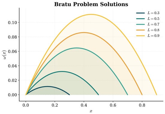
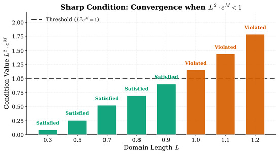
Figure 1. Solution profiles $\omega \left(x\right)$ for the Bratu problem at different domain lengths L.

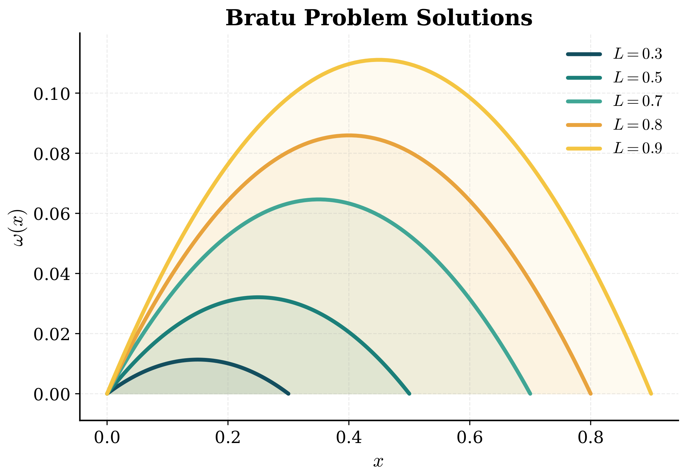
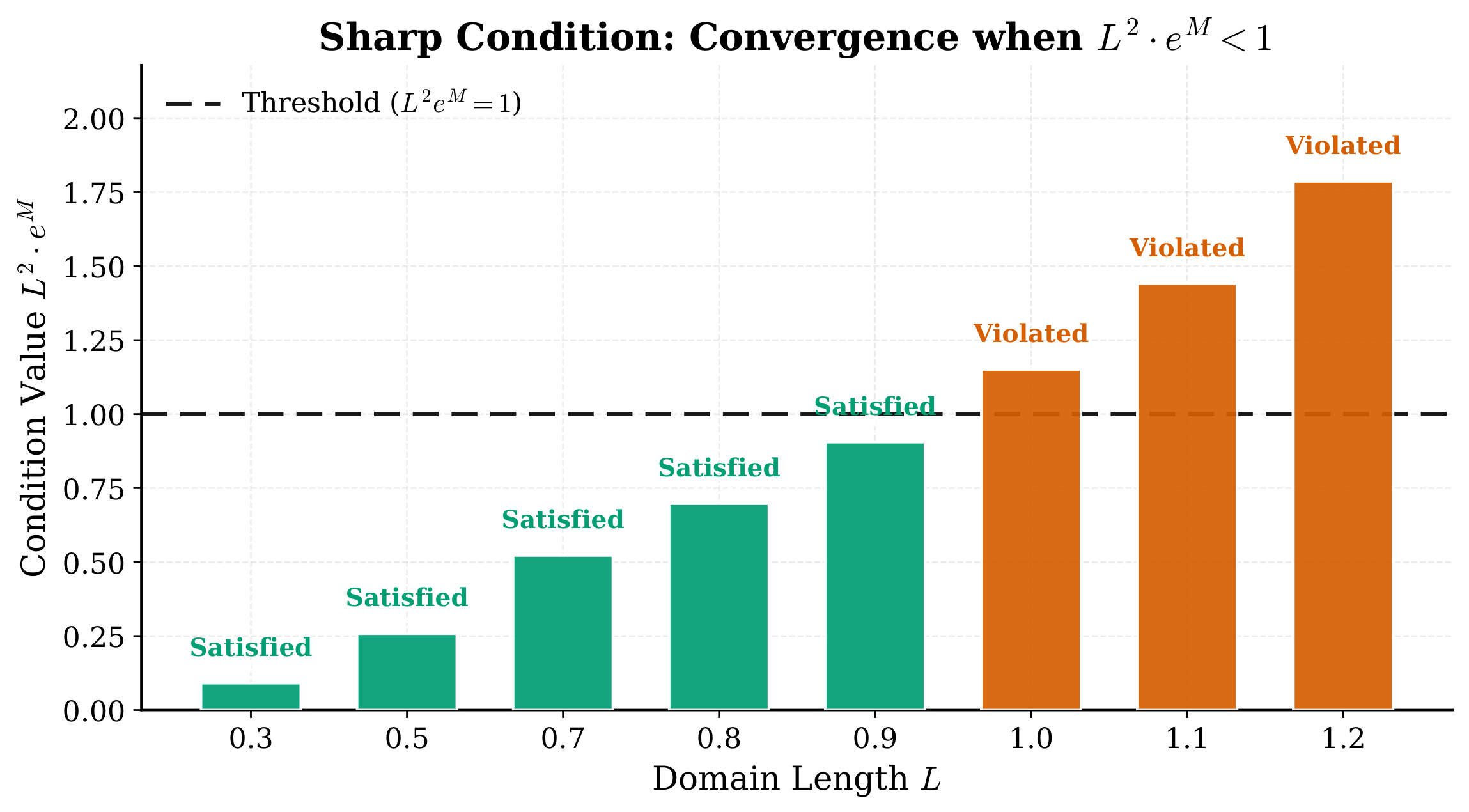
Figure 2. Verification of the sharp condition $L^2{e}^M<1$. Green bars: condition satisfied; orange bars: condition violated. The dashed line at 1 marks the theoretical threshold from Theorem 9.

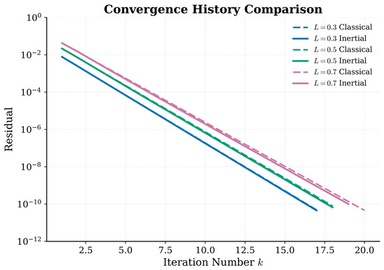
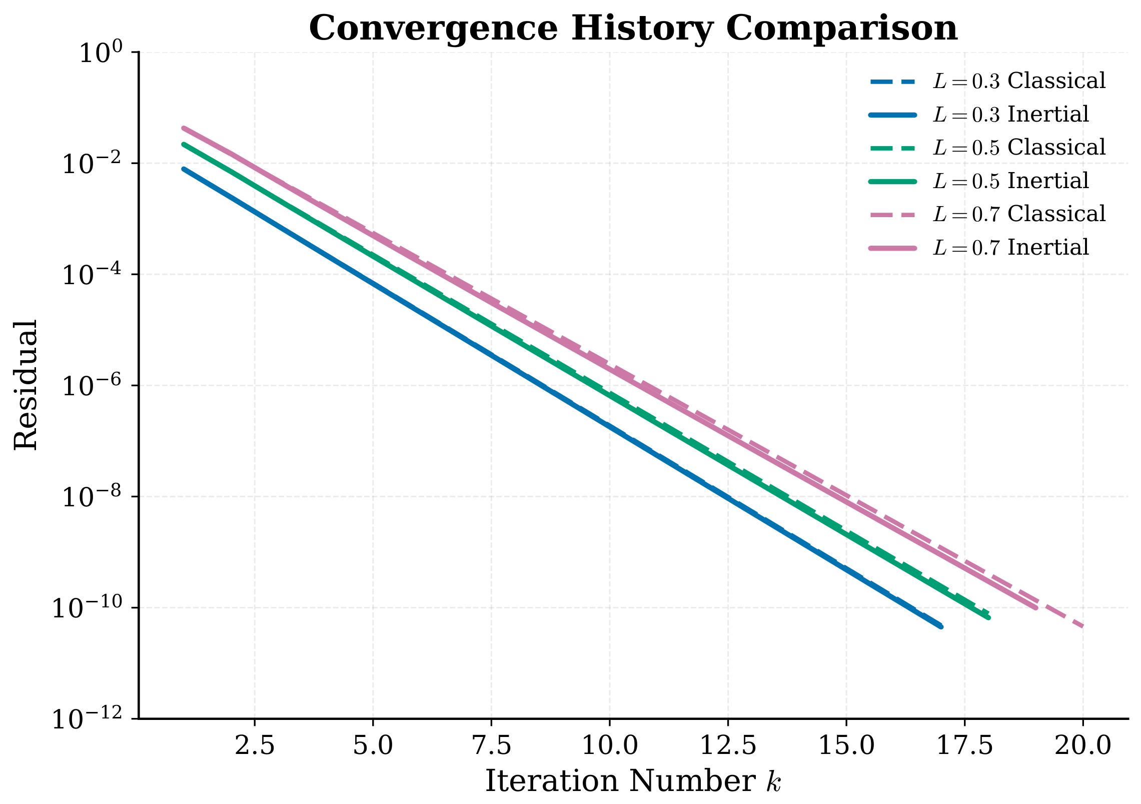
Figure 3. Convergence history comparison: residual $\parallel {\mathbf{s}}_{n+1}-{\mathbf{s}}_n{\parallel }_{\infty }$ versus iteration number n, for $L=0.3,0.5,0.7$. Inertial method (solid) shows accelerated convergence over classical method (dashed).

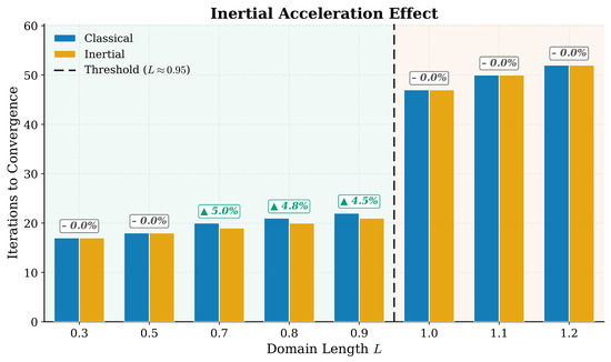
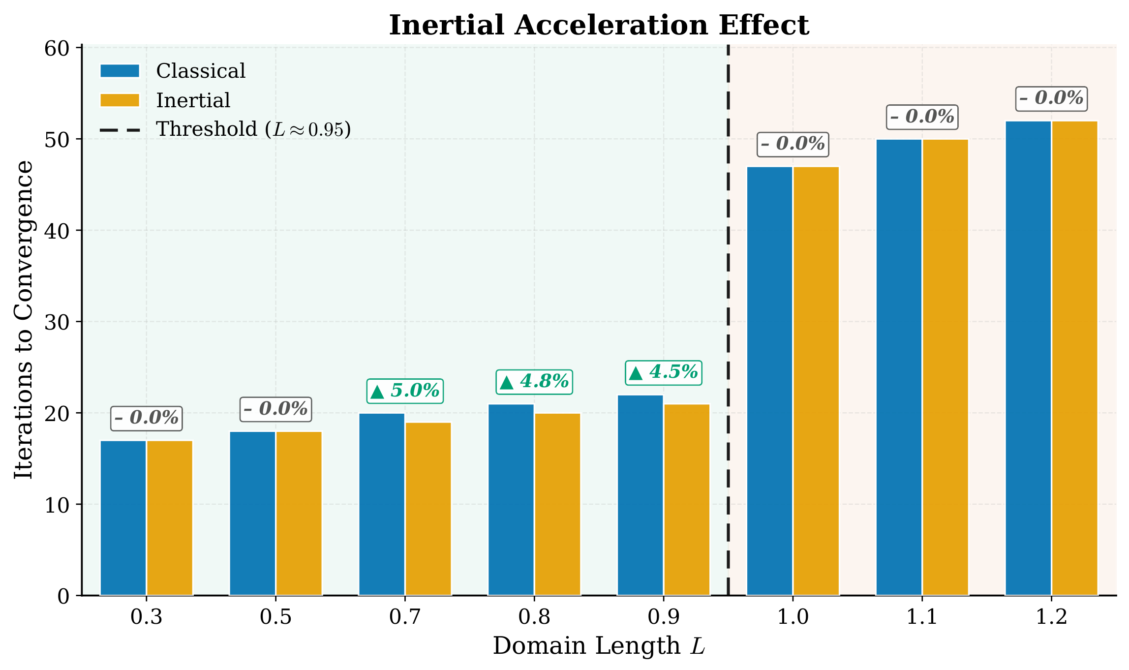
Figure 4. Iteration count comparison between classical and inertial methods. The inertial method achieves up to $5.0\%$ speedup at $L=0.7,0.8,$ and $0.9$; at the remaining tested domain lengths the two methods converge in the same number of iterations.

According to Theorem 9, the fixed-point mapping is contractive if and only if

$$L^2{e}^M<1,\mathrm{where}M={\parallel \omega \parallel }_{L^{\infty }(0,L)}.$$

(78)

In contrast to the abstract existence and uniqueness theory of Section 3, which holds for every $\alpha >0$ with no relative-size condition, this is the problem-specific sharp condition established in Proposition 2 for the concrete map $\mathsf{\Psi }\left(\omega \right)={\mathcal{A}}^{-1}\left(e^{\omega }\right)$.

Figure 1 displays the solution profiles $\omega \left(x\right)$ for various domain lengths L. As L increases, the solution amplitude grows and the peak becomes sharper. When L exceeds the threshold $L\approx 0.95$, the solution approaches blow-up behavior.

Figure 2 verifies the critical condition $L^2{e}^M<1$. The horizontal dashed line at 1 marks the theoretical threshold. Green bars indicate satisfied condition (fast convergence, 17–22 iterations); red bars indicate violated condition (slow convergence, 47–52 iterations).

Figure 3 compares the convergence history of classical and inertial methods for $L=0.3,0.5,0.7$. The inertial method (solid lines) exhibits faster residual decay than the classical method (dashed lines), with the improvement most pronounced when the contraction condition is strongly satisfied ($L=0.3$). The residual is measured as $\parallel {\mathbf{s}}_{n+1}-{\mathbf{s}}_n{\parallel }_{\infty }$.

Figure 4 provides a direct iteration count comparison. In the contractive regime ($0.3\le L\le 0.9$), the inertial method requires strictly fewer iterations at $L=0.7,0.8,0.9$ (a speedup of $4.5$–$5.0\%$), while at $L=0.3$ and $L=0.5$, classical and inertial converge in the same integer number of iterations. Both methods require significantly more iterations when the condition is violated ($L\ge 1.0$), where the inertial benefit is absent for the tested cases.

For the sake of convenience, Table 1 provides numerical results for the Bratu obstacle problem with different grids. The results in that table lead to the following conclusions:

• When $L^2{e}^M<1$ (rows above the midrule), the contraction condition is satisfied. Convergence is rapid (17–22 iterations). The inertial method achieves a measurable speedup ($4.5$–$5.0\%$) at $L=0.7,0.8,$ and $0.9$, while at $L=0.3$ and $L=0.5$, both methods converge in the same integer number of iterations.
• When $L^2{e}^M>1$ (rows below the midrule), the condition is violated. Convergence slows dramatically (47–52 iterations), and the inertial method shows no measurable benefit at any of the three violated-condition domain lengths tested.
• The threshold occurs at $L\approx 0.95$, providing direct numerical validation of Theorem 9.

Summarizing, the numerical results obtained in this work provide strong empirical support for our theoretical framework:

• Sharp condition validation: The transition at $L^2{e}^M=1$ precisely matches the problem-specific contraction threshold of Proposition 2 and Theorem 9. Convergence is fast (17–22 iterations) when the condition holds and slow (47–52 iterations) when it fails.
• Inertial acceleration: In the contractive regime, the two-step inertial method reduces iteration counts by up to $5.0\%$, but only at $L=0.7,0.8,$ and $0.9$, confirming Theorem 7; at the remaining five tested domain lengths ($L=0.3,0.5,1.0,1.1,1.2$) the classical and inertial iteration counts coincide, since both round to the same integer number of steps required to reach the tolerance. The inertial iterates never require more steps than the classical ones at any tested domain length.
• Parameter robustness: The decaying inertial parameter ${\Delta }_n={\Delta }_0/{(n+1)}^{0.8}$ satisfies the summability condition ${\sum }_{n=1}^{\infty }{\Delta }_n{\parallel {\mathbf{s}}_n-{\mathbf{s}}_{n-1}\parallel }_{\mathfrak{X}}<\infty$, ensuring convergence as proven in Lemma 5.
• Threshold behavior: The sharp change in convergence behavior at $L\approx 0.95$ validates the problem-specific contraction threshold of Proposition 2 and Theorem 9; uniqueness of the solution itself (Theorem 5) holds regardless of L.

These findings confirm that the two-step inertial method is both mathematically justified and computationally efficient for solving EVIs (1) when the contraction condition is satisfied.

6. Conclusions

This paper presented a comprehensive study of EVIs (1) and their numerical solution through an inertial acceleration strategy. We showed that the exponential nonlinearity is the gradient of a convex functional, hence monotone (Lemma 3), and used this fact to establish that the EVIs (1) has a unique solution, and that the fixed-point mapping ${\mathsf{\Psi }}_{\tau }$ defined in (14) is a contraction for an explicit, computable step-size range, for every strong monotonicity constant $\alpha >0$ of $\mathcal{A}$, with no relative-size condition against the exponential term. Comprehensive existence theorems were also obtained via boundary conditions, coercivity, and monotonicity, leading to the fixed-point theorem (Theorem 6).

We designed a two-step inertial predictor–corrector scheme Algorithm 1 with inertial extrapolation ${\psi }_n={\omega }_n+{\Delta }_n({\omega }_n-{\omega }_{n-1})$, a following projection step to ensure feasibility, and relaxation ${\rho }_n$, extending classical projection methods. A key improvement from standard formulations is the use of a distinct predictor variable ${\psi }_n$ that does not replace the current iterate ${\omega }_n$.

Using the non-expansive projection property (Lemma 2) and Xu’s lemma (Lemma 5), we established strong convergence of the inertial iterates to the unique solution ${\omega }^{*}$ under the summability condition ${\sum }_{n=1}^{\infty }{\Delta }_n{\parallel {\omega }_n-{\omega }_{n-1}\parallel }_{\mathfrak{X}}<\infty$ (Theorem 7). For constant parameters, we obtained linear convergence with rate $1-\rho (1-\theta )$ (Corollary 2).

The Bratu-type obstacle problem (46) was analyzed within our framework, demonstrating correspondence to minimization and fixed-point Equations (Theorem 8). The concrete sharp condition ${(b-a)}^2{e}^M<1$ was established, ensuring existence, uniqueness, and strong convergence of the inertial scheme (Theorem 9). Numerical simulations supported the theoretical findings, showing that the two-step inertial method provides a noticeable rise of up to $5\%$ in the contractive regime’s mid-range ($L=0.7,0.8,0.9$), while neither the non-contractive regime nor the shortest examined domain lengths showed any visible improvement.

Finally, prospective directions for future research include (i) adaptive parameter selection techniques for the relaxation parameters ${\rho }_n$ and inertial coefficients ${\Delta }_n$; (ii) extension to stochastic EVIs; (iii) multi-dimensional finite element discretizations of the presented method; (iv) investigation of quasi-variational inequalities with exponential nonlinearities; and (v) integration of deep learning techniques to improve the fixed-point iterations.

References

- Stampacchia, G. Formes bilineaires coercitives sur les ensembles convexes. Comptes Rendus Acad. Sci. Paris 1964, 258, 4413–4416. [Google Scholar]
- Lions, J.L.; Stampacchia, G. Variational inequalities. Commun. Pure Appl. Math. 1967, 20, 493–512. [Google Scholar] [CrossRef] [Scilit]
- Cottle, R.W.; Pang, J.S.; Stone, R.E. The Linear Complementarity Problem; Academic Press: New York, NY, USA, 1992. [Google Scholar]
- Glowinski, R.; Lions, J.J.; Tremolieres, R. Numerical Analysis of Variational Inequalities; North-Holland: Amsterdam, The Netherlands, 1981. [Google Scholar]
- Patriksson, M. Nonlinear Programming and Variational Inequality Problems: A Unified Approach; Kluwer Academic Publishers: Dordrecht, The Netherlands, 1998. [Google Scholar]
- Jabeen, S.; Macías, S.; Ullah, S.; Noor, M.A.; Macías-Díaz, J.E. Note on an inertial projection-based approach for solving extended general quasi-variational inequalities and its convergence analysis. Appl. Numer. Math. 2025, 217, 190–198. [Google Scholar] [CrossRef] [Scilit]
- Jabeen, S.; Macías, S.; Macías-Díaz, J.E.; Ullah, S. Convergence analysis of an inertial method for a system of general quasi-variational inequalities under mild conditions. Acta Comment. Univ. Tartu. Math. 2025, 29, 243–258. [Google Scholar] [CrossRef] [Scilit]
- Noor, M.A.; Oettli, W. On general nonlinear complementarity problems and quasi equilibria. Matematiche 1994, 49, 313–331. [Google Scholar]
- Bratu, G. Sur les équations intégrales non linéaires. Bull. Soc. Math. Fr. 1914, 42, 113–142. [Google Scholar] [CrossRef] [Scilit]
- Keshavarz, E.; Ordokhani, Y.; Razzaghi, M. The Taylor wavelets method for solving the initial and boundary value problems of Bratu-type equations. Appl. Numer. Math. 2018, 128, 205–216. [Google Scholar] [CrossRef] [Scilit]
- Li, P.; Qiao, R.; Xu, C.; Yao, M.; Qu, Y. Physics-informed symbolic regression and Haar wavelet approaches to study a new fractional-order 3D chaotic system with no equilibrium. Chaos 2026, 36, 023117. [Google Scholar] [CrossRef] [Scilit] [PubMed]
- Ben-Israel, A.; Mond, B. What is invexity? J. Aust. Math. Soc. Ser. B 1986, 28, 1–9. [Google Scholar] [CrossRef] [Scilit]
- Hanson, M.A. On sufficiency of the Kuhn-Tucker conditions. J. Math. Anal. Appl. 1981, 80, 545–550. [Google Scholar] [CrossRef] [Scilit]
- Mohan, S.R.; Neogy, S.K. On invex sets and preinvex functions. J. Math. Anal. Appl. 1995, 189, 901–908. [Google Scholar] [CrossRef] [Scilit]
- Weir, T.; Mond, B. Preinvex functions in multiobjective optimization. J. Math. Anal. Appl. 1988, 136, 29–38. [Google Scholar] [CrossRef] [Scilit]
- Ruiz-Garzón, G.; Osuna-Gómez, R.; Rufián-Lizán, A. Generalized invex monotonicity. Eur. J. Oper. Res. 2003, 144, 501–512. [Google Scholar] [CrossRef] [Scilit]
- Yang, X.M.; Yang, Q.; Teo, K.L. Criteria for generalized invex monotonicities. Eur. J. Oper. Res. 2005, 164, 115–119. [Google Scholar] [CrossRef] [Scilit]
- Avriel, M. r-Convex functions. Math. Program. 1972, 2, 309–323. [Google Scholar] [CrossRef] [Scilit]
- Zhao, Y.X.; Wang, S.Y.; Uria, L.C. Characterizations of r-Convex functions. J. Optim. Theory Appl. 2010, 145, 186–195. [Google Scholar]
- Antczak, T. On (p,r)-invex sets and functions. J. Math. Anal. Appl. 2001, 263, 355–379. [Google Scholar] [CrossRef] [Scilit]
- Pecaric, J.; Jaksetic, J. On exponential convexity, Euler–Radau expansions and stolarsky means. Rad Hrvat. Akad. Znan. 2013, 17, 81–94. [Google Scholar]
- Bernstein, N. Sur les fonctions absolument monotones. Acta Math. 1929, 52, 1–66. [Google Scholar] [CrossRef] [Scilit]
- Cristescu, G.; Lupsa, L. Non Connected Convexities and Applications; Kluwer Academic Publisher: Dordrecht, The Netherlands, 2002. [Google Scholar]
- Alirezaei, G.; Mazhar, R. On exponentially concave functions and their impact in information theory. J. Inform. Theory Appl. 2018, 9, 265–274. [Google Scholar]
- Pal, S.; Wong, T.K. On exponentially concave functions and a new information geometry. Ann. Probab. 2018, 46, 1070–1113. [Google Scholar] [CrossRef] [Scilit]
- Noor, M.A.; Noor, K.I.; Rassias, M.T. Exponentially general convex functions and variational inequalities. In Convex and Variational Analysis with Applications; Rassias, T.M., Pardalos, P.M., Eds.; Springer Optimization and Its Applications; Springer: Cham, Switzerland, 2026; Chapter 18; pp. 363–416. [Google Scholar]
- Noor, M.A. Variational-like inequalities. Optimization 1994, 30, 323–330. [Google Scholar] [CrossRef] [Scilit]
- Noor, M.A.; Noor, K.I. Higher order strongly exponentially preinvex functions. J. Appl. Math. Inform. 2021, 39, 469–485. [Google Scholar]
- Correa, R.; López, M.; Pérez-Aros, P. Log-exponential approximation in semi-infinite programming: A variational approach. J. Nonlinear Var. Anal. 2025, 9, 539–560. [Google Scholar] [CrossRef] [Scilit]
- Raus, M.; Elshiaty, Y.; Petra, S. Accelerated Bregman divergence optimization with SMART: An information geometric point of view. J. Appl. Numer. Optim. 2024, 6, 1–40. [Google Scholar] [CrossRef] [Scilit]
- He, X.; Hu, R.; Fang, Y.P. Global and exponential convergence of a primal-dual dynamical system approach for the separable convex optimization problem. Commun. Optim. Theory 2026, 2026, 1–19. [Google Scholar] [CrossRef] [Scilit]
- Alvarez, F.; Attouch, H. An inertial proximal method for maximal monotone operators via discretization of a nonlinear oscillator with damping. Set-Valued Anal. 2000, 9, 3–11. [Google Scholar] [CrossRef] [Scilit]
- Hendy, A.S.; Pimenov, V.G.; Macías-Díaz, J.E. Convergence and stability estimates in difference setting for time-fractional parabolic equations with functional delay. Numer. Methods Partial Differ. Equ. 2020, 36, 118–132. [Google Scholar] [CrossRef] [Scilit]
- Nesterov, Y. A method for solving the convex programming problem with convergence rate O(1/k2). Dokl. Akad. Nauk SSSR 1983, 269, 543–547. [Google Scholar]
- Polyak, B.T. Some methods of speeding up the convergence of iteration methods. USSR Comput. Math. Math. Phys. 1964, 4, 1–17. [Google Scholar] [CrossRef] [Scilit]
- Shehu, Y.; Gibali, A.; Sagratella, S. Inertial projection-type method for solving quasi variational inequalities in real Hilbert space. J. Optim. Theory Appl. 2020, 184, 877–894. [Google Scholar] [CrossRef] [Scilit]
- Rockafellar, R.T. Convex Analysis; Princeton University Press: Princeton, NJ, USA, 1970. [Google Scholar]
- Zhu, D.L.; Marcotte, P. Coercivity and its role in the convergence of iterative schemes for solving variational inequalities. SIAM J. Optim. 1996, 6, 714–726. [Google Scholar] [CrossRef] [Scilit]
- Xu, H.K. Iterative algorithms for nonlinear operators. J. Lond. Math. Soc. 2002, 66, 240–256. [Google Scholar] [CrossRef] [Scilit]
Disclaimer/Publisher’s Note: The statements, opinions and data contained in all publications are solely those of the individual author(s) and contributor(s) and not of MDPI and/or the editor(s). MDPI and/or the editor(s) disclaim responsibility for any injury to people or property resulting from any ideas, methods, instructions or products referred to in the content. |
© 2026 by the authors. Licensee MDPI, Basel, Switzerland. This article is an open access article distributed under the terms and conditions of the Creative Commons Attribution (CC BY) license.