B-TGPRF: A Bayesian Temporal Graph Probabilistic Model for Calibrated Overload-Risk Forecasting in Power Transmission Grids

Abstract

Modern power transmission grids are increasingly operated under volatile load, variable generation, and near-limit line-flow conditions. In such environments, deterministic line-flow forecasting is insufficient for operational decision support because operators require calibrated risk probabilities, uncertainty intervals, and reliable early warning signals. This article proposes B-TGPRF, a Bayesian Temporal Graph Probabilistic Risk Forecaster for calibrated overload-risk forecasting in power transmission grids. The proposed framework is positioned as a hybrid probabilistic graph-temporal forecasting system rather than as a new end-to-end graph neural network; its novelty lies in the leakage-controlled sequential combination of temporal forecasting, electrical graph descriptors, calibrated Bayesian risk estimation, residual correction, and compact interval uncertainty assessment. The model integrates temporal line-flow, load, and generation features with graph-topological descriptors, operating-regime indicators, residual correction, conformal interval estimation, probability calibration, and a Bayesian risk layer. A leakage-controlled data preparation pipeline was built using an open large-scale benchmark for machine learning applications in transmission grids. The final modeling dataset contains more than 3.48 million observations, 100 selected critical lines, train-only risk thresholds, and chronological train, validation, test, and external-like scenario splits. B-TGPRF was compared with persistence baselines, linear models, Bayesian baselines, tree ensembles, boosting models, neural temporal models, and compact state-of-the-art-style temporal and graph-temporal architectures. On the strict external-like test, B-TGPRF achieved MAE = 0.3650, RMSE = 0.5478, R² = 0.9962, Brier Score = 0.0147, and ECE = 0.0064. The results show that the proposed model provides a strong overall balance between line-flow forecasting accuracy, calibrated risk estimation, compact interval prediction, and low false-positive risk-signaling, while boosting models remain highly competitive for pure risk-class detection.

1. Introduction

Power transmission grids are evolving from relatively predictable centralized infrastructures into highly dynamic, data-rich, and topology-dependent systems. Increasing electricity demand, the integration of variable renewable generation, changing load patterns, and complex cross-border interconnections push individual transmission lines closer to technical operating limits. Under these conditions, early overload-risk forecasting becomes not only a physical power-system problem but also a probabilistic decision-support task.

Traditional power-system analysis remains essential for engineering operation, but modern monitoring systems also require data-driven models that can process large volumes of time-series measurements. Machine learning approaches can capture nonlinear interactions among load, generation, and line-flow variables; however, many published methods focus mainly on point prediction or binary classification. Such outputs are insufficient in risk-sensitive operation because two forecasts with similar point values may have different reliability depending on topology, regime, and proximity to an overload threshold. A practically useful overload-risk model should therefore satisfy several requirements. First, it should represent recent temporal dynamics of load, generation, and line flows. Second, it should incorporate the graph structure of the transmission network because the condition of one line is affected by neighboring lines, bus connectivity, and network centrality. Third, it should provide calibrated probabilities, not only class labels. Fourth, it should quantify prediction uncertainty and generate interpretable risk signals that can support human operators.

This study addresses these requirements by proposing a Bayesian Temporal Graph Probabilistic Risk Forecaster (B-TGPRF). The proposed model jointly forecasts future line flow and estimates calibrated overload-risk probability. It integrates temporal encoders, graph-topological information, operating-regime features, residual correction, conformal intervals, Bayesian risk inference, and validation-based probability calibration. The approach is evaluated on a large open benchmark for machine learning applications in transmission grids using a leakage-controlled data pipeline and a strict external-like scenario test.

Unlike end-to-end graph neural network models that learn graph aggregation internally, B-TGPRF uses the electrical topology as a reproducible line-level representation and combines it with temporal memory, regime-aware features, Bayesian-style risk estimation, validation-only calibration, and conformal residual intervals. Therefore, the methodological contribution of this study is not a new graph convolutional layer, but a leakage-safe probabilistic forecasting workflow that jointly produces a point forecast, calibrated overload-risk probability, risk class, compact prediction interval, and diagnostic uncertainty score.

B-TGPRF should therefore be interpreted as a leakage-safe hybrid probabilistic workflow rather than as a replacement for modern end-to-end GNNs. Its novelty lies in the sequential coupling of temporal forecasting, electrical line–line graph descriptors, operating-regime representation, Bayesian posterior-style risk estimation, validation-only calibration, residual correction, and compact conformal interval construction within one reproducible overload-risk decision pipeline.

The main contributions of this article are as follows:

• A leakage-safe data preparation and feature-engineering pipeline for graph-temporal overload-risk forecasting in power transmission grids;
• A hybrid Bayesian temporal graph architecture that generates point forecasts, calibrated risk probabilities, risk classes, prediction intervals, and diagnostic uncertainty scores;
• A broad comparison with persistence, linear, Bayesian, ensemble, boosting, neural temporal, and compact state-of-the-art-style graph-temporal baselines;
• A strict evaluation protocol that includes chronological validation, internal testing, external-like scenario testing, ablation analysis, threshold sensitivity, and horizon sensitivity.

2. Related Work

2.1. Machine Learning for Power-System Security and Forecasting

Forecasting and security assessment in power systems have been widely studied using statistical, machine-learning, and deep-learning methods. Classical regression and probabilistic models are still useful because they are relatively simple and interpretable. However, modern transmission grids are affected by nonlinear interactions among load, generation, topology, and line flows. For this reason, recent studies emphasize that smart-grid operation requires not only accurate point forecasts, but also uncertainty-aware and probabilistic models that can support practical decision-making [1,2,3,4,5].

Tree ensembles and gradient-boosting models, such as XGBoost, LightGBM, Random Forest, and Extra Trees, are widely used as strong baselines for tabular prediction tasks [6,7,8,9]. These models can effectively use engineered temporal, graph-derived, and operating-regime features, and they often provide high accuracy in both regression and classification problems. At the same time, they do not directly model the power grid as a graph. Therefore, when such models are applied to transmission-grid problems, the network topology usually has to be represented through manually designed graph-related features.

2.2. Graph Neural Networks and Spatio-Temporal Modeling

Transmission grids naturally have a graph structure. Buses, lines, transformers, and generators are connected to each other, and changes in one part of the network may influence neighboring elements. Because of this, graph neural networks and graph-temporal models have become important tools for power-flow approximation, security assessment, fault analysis, and time-series prediction in electrical networks [10,11,12,13,14,15].

Recent benchmark studies also show that graph-based power-system models should be evaluated under realistic and safety-oriented conditions, not only by average prediction accuracy. Data-driven security assessment studies, PowerGraph, and SafePowerGraph provide useful examples of benchmark datasets and evaluation protocols for transmission-grid learning [13,14,15]. These works are relevant to the present study because B-TGPRF is evaluated not only by global accuracy, but also by external-like scenario testing, subgroup analysis, robustness checks, and safety-oriented metrics.

General graph neural network methods provide the methodological foundation for this area. Graph convolutional networks, graph attention networks, GraphSAGE, graph isomorphism networks, and general GNN surveys show how neighborhood aggregation, attention, inductive learning, and graph expressiveness can be used for structured prediction tasks [16,17,18,19,20].

Spatio-temporal graph convolutional networks and Graph WaveNet show how graph structure can be combined with temporal modeling [21,22]. In parallel, Transformers, recurrent neural networks, temporal convolutional networks, DeepAR, Temporal Fusion Transformers, PatchTST-style models, and recent time-series forecasting surveys have improved sequential and multi-horizon forecasting [23,24,25,26,27,28,29,30,31]. However, the performance of these models in power-system applications depends strongly on graph construction, data volume, forecast horizon, and calibration quality.

Most graph neural forecasting models use learned message passing over bus-level, branch-level, or equipment-level graphs. This is a powerful approach, but it may require large training datasets, careful graph design, and detailed validation of probabilistic reliability. In contrast, B-TGPRF does not propose a new graph neural layer. Instead, it uses the fixed electrical topology to build interpretable line-level graph descriptors and combines them with temporal, operating-regime, and probabilistic components. This makes the proposed model closer to a graph-informed probabilistic forecasting workflow than to a fully end-to-end GNN.

2.3. Probabilistic Forecasting, Calibration, and Conformal Prediction

For overload-risk forecasting, uncertainty-aware modeling is especially important. In practical operation, the model should not only indicate whether a line may become overloaded, but also show how reliable this warning is. Bayesian neural networks, dropout-based uncertainty estimation, deep ensembles, and calibration studies provide useful tools for estimating predictive uncertainty and improving the reliability of model probabilities [32,33,34,35]. Nevertheless, raw model scores are not automatically trustworthy probabilities. A model may achieve high accuracy and still be overconfident or underconfident in critical operating regimes.

Conformal prediction, proper scoring rules, reliability diagrams, Brier Score, Expected Calibration Error, prediction interval coverage, and classical calibration methods help evaluate whether predicted probabilities and intervals are consistent with observed outcomes [36,37,38,39,40,41,42,43]. These methods are important because a practical overload-risk model should not optimize only one metric. It should combine line-flow forecasting, calibrated risk estimation, and interval prediction.

Recent renewable-energy forecasting studies also show that rare-event-aware hybrid architectures and multi-horizon quantile forecasting can improve uncertainty-aware prediction under variable generation conditions [44,45]. Although these studies focus on photovoltaic power rather than transmission-line overload risk, they are methodologically relevant because they support the use of probabilistic, interval-based, and horizon-aware forecasting components in energy-system decision support.

2.4. Research Gap

The reviewed literature shows three main gaps. First, many forecasting models provide accurate point predictions but do not produce calibrated overload-risk probabilities. Second, graph-temporal models often focus on prediction accuracy, while calibration quality and interval reliability receive less attention. Third, leakage-safe threshold construction and external-like scenario testing are not always treated as central parts of the experimental design.

B-TGPRF is designed to address these gaps. The proposed framework combines temporal memory, graph-topological descriptors, operating-regime features, Bayesian-style risk estimation, validation-only probability calibration, residual correction, and conformal interval construction in one reproducible workflow.

In this study, overload-risk forecasting is treated as a graph-temporal probabilistic learning problem rather than as a simple binary classification task. This is important because the same predicted line-flow value may have different operational meaning depending on the line-specific threshold, graph context, regime state, and uncertainty level. Therefore, the proposed model aims to support not only accurate forecasting, but also calibrated and interpretable risk-oriented decision support.

3. Materials and Methods

The experimental basis of this study is the open benchmark dataset ‘A large synthetic dataset for machine learning applications in power transmission grids’ [46,47]. The dataset was accessed through Zenodo (CERN, Geneva, Switzerland). The dataset contains a large-scale synthetic transmission network model and long hourly time series of load, generation, and line-flow values. The topological description is provided through the network file, while load, generator, and line-flow time-series files are supplied by year and scenario suffix group.

The raw benchmark files used in this study consisted of the network topology file ‘europe_network.json’ and the 2020 time-series archives for load, generation, and line-flow observations, namely ‘loads_2020.zip’, ‘gens_2020.zip’, and ‘lines_2020.zip’. The topology file was used to extract line connectivity, line–line adjacency, topological descriptors, neighboring-line relations, centrality indicators, and branch rating information. The load, generation, and line-flow files were merged only when their year and scenario suffix groups matched, ensuring that the resulting modeling table preserved scenario consistency across all operating variables.

The dataset was selected because it supports a graph-temporal formulation of overload-risk forecasting. It contains both network topology and operating time series, which makes it possible to combine temporal dynamics with line adjacency, centrality, branch rating, and neighboring-line statistics. This is essential because overload risk cannot be fully understood by analyzing each line independently.

$$\mathcal{G}=(\mathcal{V},\mathcal{E}),l=(fro{m}_l,t{o}_l),l\in \mathcal{E}$$

(1)

$$y_{l,h}^{flow}(t)=f_l(t+h)$$

(2)

$$r_{l,h}(t)=\left\{\begin{array}{cc}1,& \mid y_{l,h}^{flow}(t)\mid \ge q_{l,train}^{95}\\ 0,& \mid y_{l,h}^{flow}(t)\mid <q_{l,train}^{95}\end{array}\right.$$

(3)

Here, $h$ denotes the forecasting horizon, $f_l\left(t\right)$ is the signed flow of line $l$ at time $t$, $f_l\left(h\right)$ is the future line-flow target, and $q_{l,train}^{95}$ is the line-specific 95th percentile of absolute flow calculated only from the training subset. This train-only threshold prevents leakage from validation, test, and external-like scenario data. Table 1 summarizes the main structural characteristics of the transmission-grid model used in this study, including the numbers of buses, transmission lines, generators, load nodes, countries, and the range of branch ratings.

Table 1. Summary of the transmission-grid model.

No.	Indicator	Value
1	Buses	4097
2	Branches/transmission lines	8375
3	Generators	815
4	Load nodes	4097
5	Generator type count	27
6	Country count	26
7	Branch rating minimum	1.4
8	Branch rating median	4.9
9	Branch rating maximum	54.0

The scale of the network, including 4097 buses and 8375 branches, justifies the use of graph-derived features. The range of branch ratings also indicates heterogeneous line capacities, which is relevant for near-threshold and overload-risk analysis.

3.1. Graph Representation

The graph used in this study is an electrical transmission network graph rather than a geographical graph. The original network contains buses and transmission branches. For modeling purposes, this topology is converted into a line–line graph, where each monitored transmission line is represented as a node. An edge between two line nodes is created when the corresponding transmission branches share at least one common electrical bus. Thus, graph connectivity reflects electrical adjacency rather than geographical distance.

The topology is treated as fixed during the experiment because the benchmark provides a static network structure for the considered scenario groups. Operating conditions such as load, generation, and line-flow values vary over time, whereas the adjacency structure remains unchanged. Geographic coordinates are retained only as metadata and are excluded from trainable features to avoid coordinate-based leakage.

Graph information is used through reproducible descriptors rather than end-to-end neural message passing. These descriptors include line degree, centrality, branch rating information, neighboring-line-flow aggregates, graph-smoothed flow, and adjacent-line risk indicators. This design improves interpretability and reproducibility while still allowing the model to incorporate topological context into overload-risk forecasting.

Table 2 summarizes the main structural properties of the electrical line–line graph used in B-TGPRF, including the node definition, edge-construction rule, topology type, graph density, degree statistics, weighting strategy, and the way graph information enters the model.

Table 2. Description of the electrical line–line graph structure.

Parameter	Value
Graph type	Electrical line–line graph
Nodes	100 selected critical lines
Edge rule	Two lines are adjacent if they share a common electrical bus
Topology	Fixed topology
Geographical graph	No
Number of edges	125
Density	0.0253
Degree min/mean/median/max	0/2.5/2/6
Weighting	Binary adjacency + rating-weighted sensitivity
Use in model	Graph descriptors, neighbor-flow aggregation, graph-smoothed features

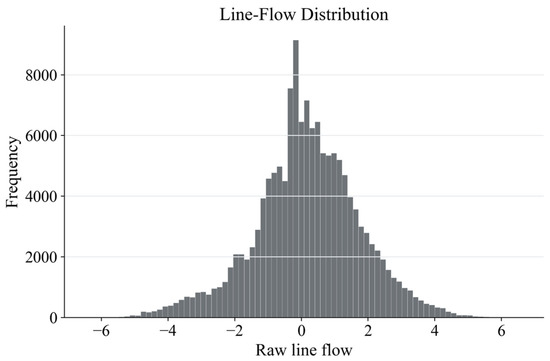
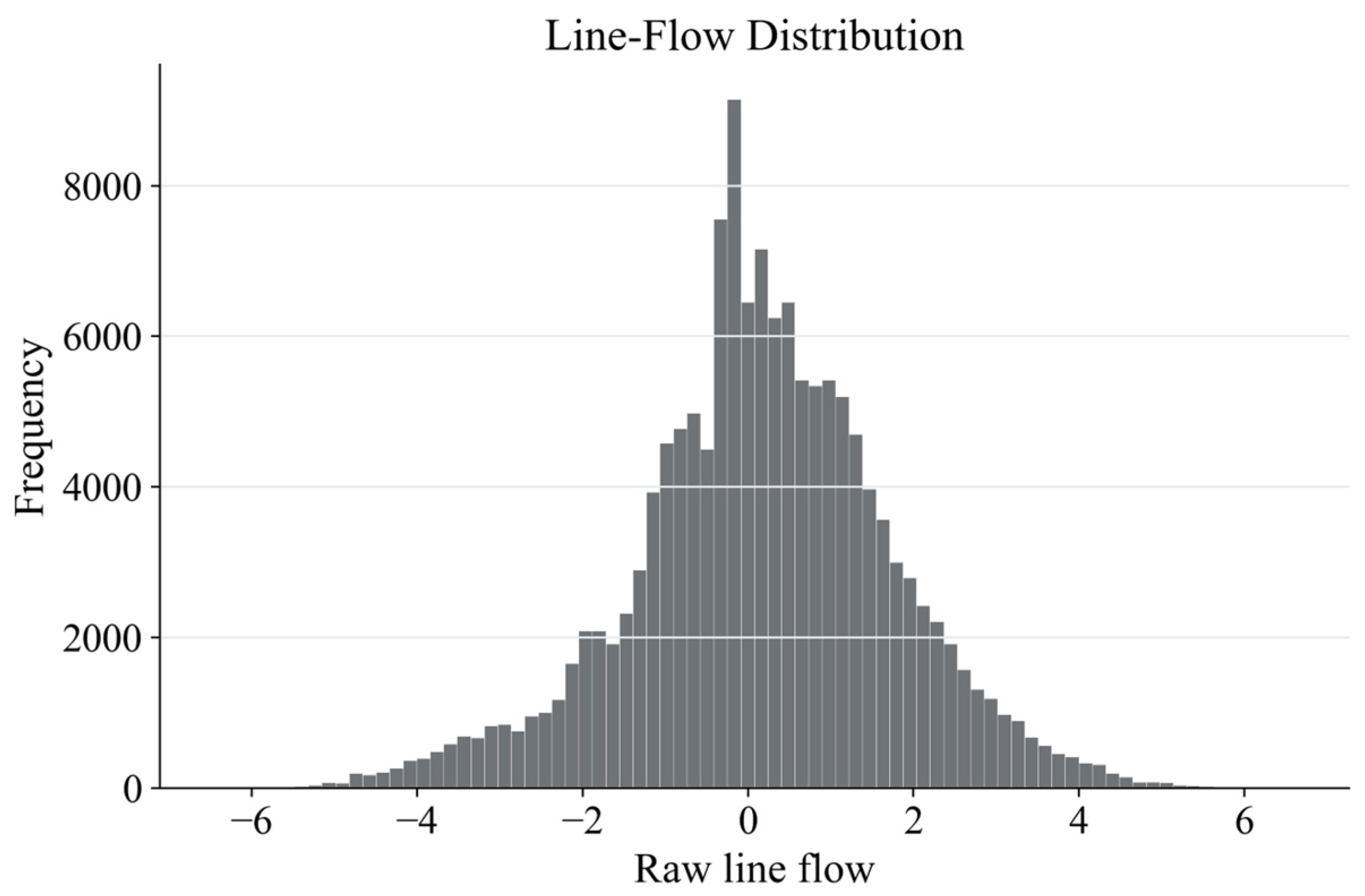
The main experiments use binary electrical adjacency. Branch rating information is not used as a geographical distance proxy; it is treated as static electrical metadata and is additionally used in a rating-weighted adjacency sensitivity check. Figure 1 shows the distribution of raw signed line-flow values in the transmission-grid dataset. The distribution is centered close to zero and has extended positive and negative tails, indicating that both flow direction and magnitude are relevant for overload-risk forecasting.

Figure 1. Distribution of raw signed line-flow values in the transmission-grid dataset.

3.2. Data Preparation and Feature Engineering

The data preparation pipeline was designed to preserve chronological structure, avoid coordinate leakage, and ensure that all thresholds, normalization parameters, and risk labels were generated only from permissible training information. Longitude and latitude were retained as metadata but excluded from trainable features to avoid artificial geographic leakage.

Raw inputs included the network topology file and yearly ZIP files containing load, generation, and line-flow time series. Files were audited for size, missing values, numeric ranges, and matching year/suffix groups. Load, generation, and line-flow groups were merged only when they shared the same year and suffix. This rule is important because scenario groups are not interchangeable.

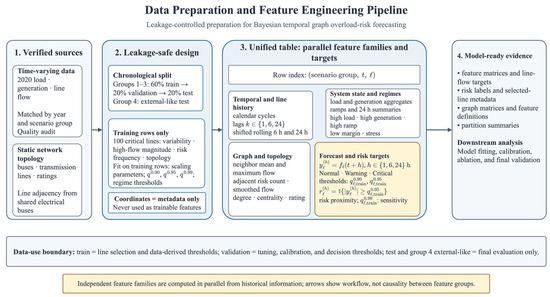
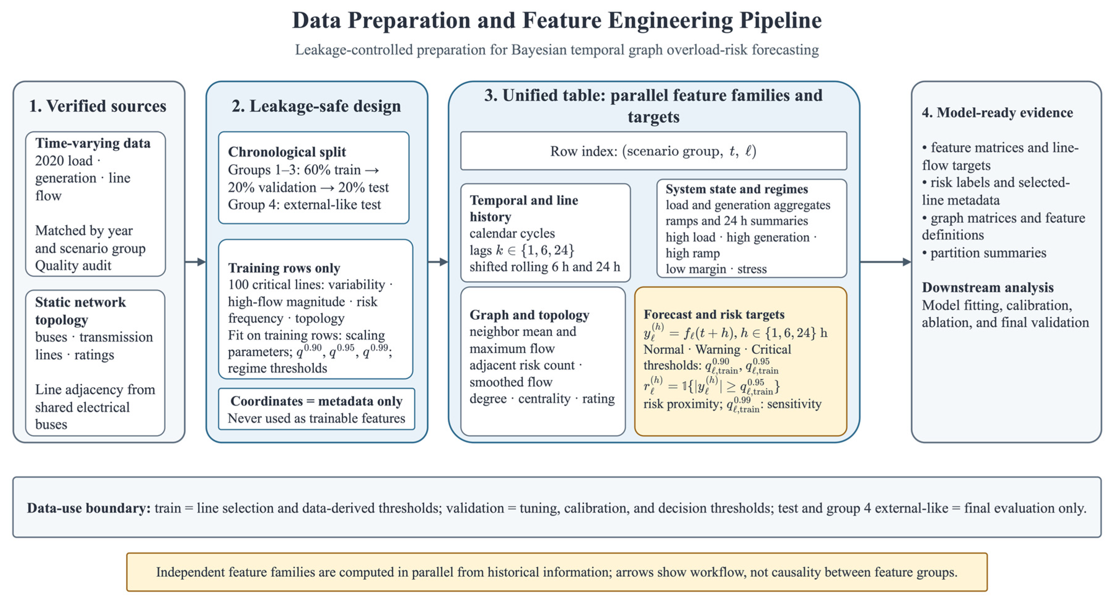
Figure 2 summarizes the leakage-controlled data preparation and feature-engineering pipeline. The pipeline starts from verified time-varying data and static network topology, applies chronological splitting and train-only threshold construction, and produces model-ready feature matrices, targets, graph matrices, selected-line metadata, and partition summaries.

Figure 2. Data preparation and feature-engineering pipeline for Bayesian temporal graph overload-risk forecasting.

The diagram emphasizes the data-use boundary of the study: training rows are used for line selection, scaling parameters, and data-derived thresholds; the validation subset is used for tuning, calibration, and decision-threshold selection; and the internal test and group 4 external-like scenario data are reserved only for final evaluation.

Feature groups include cyclic time encodings, lagged and rolling line-flow statistics, load and generation aggregates, graph-neighborhood variables, centrality and rating descriptors, operating-regime indicators, and train-only quantile-based risk proximity. The complete feature dictionary, including the feature origin, leakage-control rule, and corresponding B-TGPRF component, is reported in Supplementary Table S6. The final output of the pipeline consists of feature matrices, line-flow targets, risk labels, selected-line metadata, graph matrices, feature dictionaries, and split summaries.

The modeling table is indexed by timestamp, scenario group, and line identifier. Critical lines were selected using variability, high-flow magnitude, risk-event frequency, and topological importance. This selection focuses the analysis on the most informative elements while keeping the experiment computationally stable.

$$g_l(t)={\displaystyle \frac{1}{\mid \mathcal{N}(l)\mid }}\sum _{m\in \mathcal{N}(l)}\mid f_m(t)\mid$$

(4)

$$\mathcal{D}={\mathcal{D}}_{train}\cup {\mathcal{D}}_{val}\cup {\mathcal{D}}_{test}\cup {\mathcal{D}}_{ext}$$

(5)

Table 3 summarizes the experimental configuration and leakage-control protocol used in the study, including the data source, scenario groups, selected lines, forecast horizons, train-only risk thresholds, chronological split, and external-like scenario test.

Table 3. Experimental configuration and leakage-control protocol.

Configuration Block	Value	Purpose
Data source	Zenodo benchmark record 13378476	Open reproducible benchmark
Year used	2020	Primary modeling period
Matched suffix groups	2020 groups 1–4	Scenario-consistent merging
Selected critical lines	100	Risk-informative subset
Forecast horizons	1, 6, and 24 h	Short- and medium-horizon assessment
Risk thresholds	q90, q95, q99	Warning and critical risk levels
Main risk threshold	q95 train-only absolute flow	Primary binary risk label
Train/validation/test	60%/20%/20% of groups 1–3	Chronological model selection and internal testing
External-like test	All valid target times in group 4	Strict scenario-level robustness check

Table 4 reports the leakage audit of the experimental pipeline. Since the reported forecasting accuracy is high, an additional audit was performed to verify that no future or external-test information was used during model training, preprocessing, risk-threshold construction, probability calibration, or interval estimation. The purpose of this audit is to document the main safeguards of the pipeline and to demonstrate that all model-development decisions were based only on the training or validation subsets, while the internal test and external-like scenario test were kept fully held out.

Table 4. Leakage audit of the experimental pipeline.

Check	Leakage-Control Rule	Status
Chronological split	Training, validation, and test subsets follow temporal order	Passed
External-like scenario	Group 4 is not used for training, model selection, scaling, thresholding, or calibration	Passed
Risk thresholds	q90, q95, and q99 are computed only from training rows	Passed
Scaling parameters	Normalization parameters are fitted only on the training subset	Passed
Calibration	Probability calibration is fitted only on the validation subset	Passed
Future target exclusion	Future line-flow values are used only as targets, not as input features	Passed
Lag and rolling features	Lagged and rolling features use only current and past observations	Passed

This audit does not claim that high forecasting accuracy alone proves the absence of leakage. Rather, it documents the main safeguards used to reduce information leakage risk: chronological splitting, train-only threshold estimation, train-only scaling, validation-only calibration, validation-only conformal correction, and exclusion of future target values from the input feature set.

3.3. Proposed B-TGPRF Method

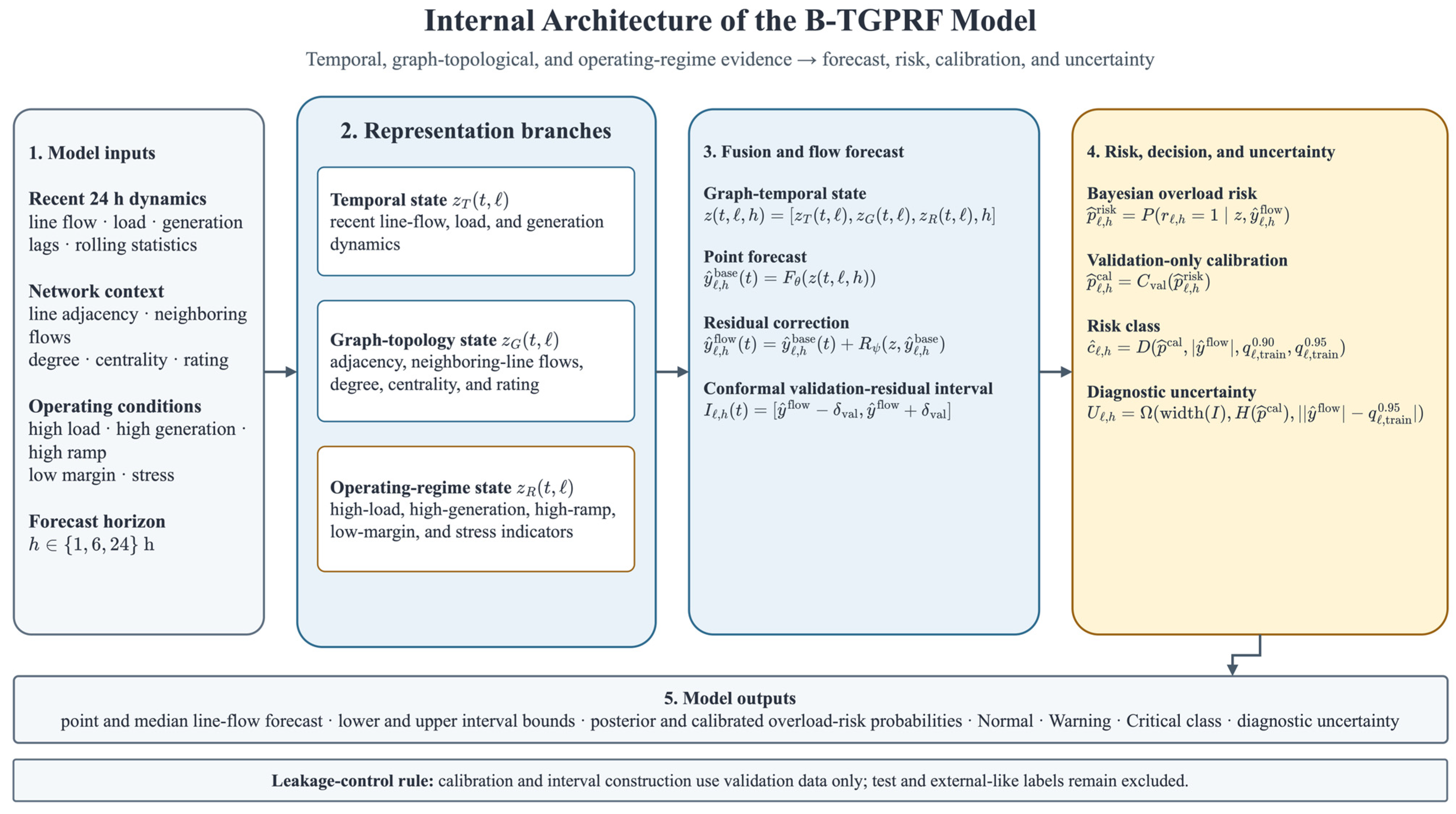
B-TGPRF consists of three representation branches followed by graph-temporal fusion, a forecasting backbone, residual correction, conformal interval estimation, Bayesian risk inference, calibration, and diagnostic uncertainty estimation. This design reflects the assumption that overload risk is generated by interacting temporal, topological, and operating-regime factors.

The temporal branch summarizes recent 24 h dynamics of line flow, load, generation, lags, and rolling features. The graph-topology branch uses line adjacency, neighboring-line flows, centrality, degree, and branch rating information. The regime branch encodes high-load, high-generation, high-ramp, low-margin, and stress indicators.

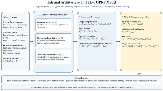
Figure 3 illustrates the internal architecture of B-TGPRF. The model receives recent 24 h temporal dynamics, network-context features, operating-condition indicators, and the forecast horizon as inputs. These inputs are transformed into temporal, graph-topological, and operating-regime representations, which are then fused for line-flow forecasting, residual correction, conformal interval construction, Bayesian overload-risk estimation, validation-only calibration, risk classification, and diagnostic uncertainty scoring.

Figure 3. Internal architecture of the B-TGPRF model.

The architecture is intentionally organized as a sequential probabilistic workflow rather than as a fully end-to-end graph neural network. This design makes the use of temporal evidence, graph-topological descriptors, operating-regime indicators, calibration, and uncertainty estimation explicit and reproducible.

The internal structure of B-TGPRF consists of several related branches. The temporal branch processes the dynamics of line flows, load, and generation:

$$z_T(t,l)=E_T\left(x_{t-L,l},\dots ,x_{t,l}\right)$$

(6)

The graph-topological branch uses the adjacency matrix of lines and features of neighboring elements:

$$z_G(t,l)=E_G\left(A_L,\{x_{t,m}:m\in \mathcal{N}(l)\}\right)$$

(7)

The regime branch encodes signs of high consumption, high generation, abrupt flow changes, and proximity to threshold states:

$$z_R(t,l)=E_R\left(regim{e}_{t,l}\right)$$

(8)

After that, the three views are combined into a single graph-temporal state of the model:

$$z(t,l,h)=[z_T(t,l),z_G(t,l),z_R(t,l),h]$$

(9)

Based on the combined state, a point forecast of the future flow is constructed:

$${\widehat{y}}_{l,h}^{base}(t)=F_{\theta }(z(t,l,h))$$

(10)

For more accurate processing of near-threshold and high-risk modes, we add residual correction:

$${\widehat{y}}_{l,h}^{flow}(t)={\widehat{y}}_{l,h}^{base}(t)+R_{\psi }(z(t,l,h),{\widehat{y}}_{l,h}^{base}(t))$$

(11)

where $R_{\psi }$ corrects the error of the base forecast in modes close to the overload threshold.

The Bayesian risk layer translates the graph-temporal state and adjusted forecast into a posterior overload probability:

$${\widehat{p}}_{l,h}^{risk}(t)=P(r_{l,h}(t)=1\mid z(t,l,h),{\widehat{y}}_{l,h}^{flow}(t))$$

(12)

In this study, the term Bayesian risk layer is used in an applied probabilistic sense. It denotes a component that maps the graph-temporal state, residual-corrected line-flow forecast, and proximity to train-only risk thresholds into a posterior-style overload-risk probability. B-TGPRF is not intended to be interpreted as a full Bayesian neural network with prior distributions over all weights and full posterior inference over model parameters. The Bayesian component is used for posterior-style risk estimation and is followed by validation-only probability calibration to reduce overconfidence and improve probabilistic interpretability.

Next, the probability is calibrated on the validation part:

$${\widehat{p}}_{l,h}^{cal}(t)=C_{val}\left({\widehat{p}}_{l,h}^{risk}(t)\right)$$

(13)

where $C_{val}(\cdot )$ is the calibration transformation constructed without using the test and external-test parts.

The interval forecast is formed using a conformal correction based on the distribution of validation residuals:

$$I_{l,h}(t)=\left[{\widehat{y}}_{l,h}^{flow}(t)-{\delta }_{val},{\widehat{y}}_{l,h}^{flow}(t)+{\delta }_{val}\right]$$

(14)

where ${\delta }_{val}$ is calculated from the distribution of validation residuals.

The final risk class is determined using the calibrated probability and threshold proximity to the critical level:

$${\widehat{c}}_{l,h}(t)=D\left({\widehat{p}}_{l,h}^{cal}(t),\mid {\widehat{y}}_{l,h}^{flow}(t)\mid ,q_{l,train}^{90},q_{l,train}^{95}\right)$$

(15)

where $D (\cdot )$ sets the Normal/Warning/Critical solution.

Diagnostic uncertainty combines three sources: the interval width, the posterior probability entropy, and the proximity of the forecast to the overload threshold:

$$U_{l,h}(t)=\mathsf{\Omega }\left(width(I_{l,h}(t)),H({\widehat{p}}_{l,h}^{cal}(t)),\mid \mid {\widehat{y}}_{l,h}^{flow}(t)\mid -q_{l,train}^{95}\mid \right)$$

(16)

Thus, the B-TGPRF generates not only a forecast of the future flow, but also a probabilistic risk assessment, a risk class, an uncertainty interval, and a diagnostic confidence indicator. This makes the model suitable for tasks where not only the accuracy of the prediction is important, but also an interpreted estimate of the risk of overload.

The detailed probability calibration protocol, including the calibration input, validation-only fitting rule, Brier Score formula, ECE formula, and binning strategy, is reported in Supplementary Table S1.

The final model output includes a point and median line-flow forecast, lower and upper probabilistic bounds, posterior and calibrated overload-risk probabilities, a Normal/Warning/Critical decision, and a diagnostic uncertainty score. The calibration function $C_{val}$ is fitted on the validation subset and is not allowed to use test or external-like scenario labels.

The interval construction protocol, residual definition, empirical compact interval level, and leakage-control rule are provided in Supplementary Table S3. The reported B-TGPRF interval should be interpreted as a compact empirical predictive interval rather than as a 95% safety envelope.

The complete B-TGPRF workflow consists of leakage-controlled data preparation, construction of temporal, graph-neighborhood, and operating-regime features, train-only risk-threshold estimation, graph-temporal representation learning, residual-corrected line-flow forecasting, Bayesian overload-risk estimation, validation-based probability calibration, conformal interval construction, and diagnostic uncertainty scoring. These components are described in the following subsections and summarized visually in Figure 2 and Figure 3.

3.4. Experimental Setup

The proposed model was evaluated against multiple model families. The comparison was intentionally broad to avoid testing B-TGPRF only against weak baselines. For neural temporal and graph-temporal models, compact implementations inspired by state-of-the-art architectures were used; therefore, the results should not be interpreted as claims against full industrial-scale implementations of every architecture.

The comparative design was organized by model families rather than by isolated algorithms (Table 5). Persistence models define the minimum acceptable forecasting baseline; linear and Bayesian baselines test whether the task can be solved by simple interpretable dependencies; tree ensembles and boosting methods provide strong nonlinear tabular competitors; neural temporal models test sequential representation learning; compact graph-temporal models assess the value of explicit temporal–topological representation; and probabilistic interval models provide a benchmark for uncertainty-aware forecasting. This structure allows B-TGPRF to be evaluated against models of different complexity and modeling assumptions.

Table 5. Model families used in the comparative study.

Family	Models	Main Role
Persistence baselines	Persistence; seasonal previous-day persistence	Lower-bound forecasting and risk baselines
Linear and Bayesian baselines	Ridge; ElasticNet; logistic regression; Gaussian Naive Bayes; Bayesian Ridge approximation	Interpretable regression and probabilistic baselines
Tree ensembles and boosting	Random Forest; Extra Trees; HistGradientBoosting; XGBoost; LightGBM	Strong nonlinear tabular baselines
Neural temporal models	LSTM; GRU; TCN; Transformer Encoder	Sequential line-flow and risk modeling
Compact SOTA-style graph-temporal models	STGCN-inspired; Graph WaveNet-inspired; PatchTST-style; TFT-inspired attention	Temporal and graph-temporal representation testing
Probabilistic interval models	Quantile Gradient Boosting conformal baseline	Prediction interval comparison
Proposed model	B-TGPRF	Joint line-flow forecasting, calibrated risk estimation, and uncertainty quantification

To improve the fairness of comparison, all models were trained and evaluated using the same chronological split, the same external-like scenario test, the same target definitions, and the same leakage-controlled preprocessing rules. The validation subset was used for model selection, threshold selection, calibration, or early stopping where applicable. The test and external-like scenario subsets were not used for training, scaling, calibration, conformal residual estimation, or hyperparameter selection.

Table 6 reports the fairness and hyperparameter-control protocol used for the strongest competing models and the proposed B-TGPRF framework. The table shows that all models were trained on the same number of rows, used the same random seed where applicable, and were evaluated under the same chronological validation protocol.

Table 6. Fairness and hyperparameter-control protocol.

Model	Train Rows	Random Seed	Validation Protocol	HPO/Selection
HistGradientBoostingClassifier	1,572,300	42	Chronological validation	Limited equal-budget search
LightGBM	1,572,300	42	Chronological validation	Limited equal-budget search
XGBoost	1,572,300	42	Chronological validation	Limited equal-budget search
Extra Trees	1,572,300	42	Chronological validation	Limited equal-budget search
B-TGPRF	1,572,300	42	Validation-only calibration/selection	Component selection

To improve the reproducibility of the compact neural and graph-temporal baselines, the main architectural and training settings are reported in Supplementary Table S18. These settings include the lookback window, number of input features, hidden dimension, optimizer, loss function, row limits, early stopping rule, and architecture-specific details. The neural baselines should be interpreted as compact SOTA-style implementations under a controlled benchmark budget rather than as full industrial-scale implementations.

For computational feasibility, a limited equal-budget hyperparameter search was applied to the strongest tabular and boosting baselines. Neural and graph-temporal baselines were implemented as compact SOTA-style variants; therefore, the comparison should be interpreted as a controlled benchmark comparison rather than an exhaustive industrial-scale optimization of every architecture.

Classification metrics included accuracy, Balanced Accuracy, Macro-F1, Weighted-F1, precision, recall, specificity, false-positive rate, false-negative rate, ROC-AUC, and PR-AUC. Forecasting metrics included MAE, RMSE, sMAPE, MAPE_safe, ramp_MAE, R², and normalized RMSE. Calibration and interval quality were evaluated using Brier Score, Expected Calibration Error, pinball loss, interval coverage, mean interval width, and uncertainty–error correlation.

4. Results

4.1. External-Test Classification Performance

Table 7 summarizes the strict external-like test classification results for the most relevant models. Boosting models achieved the strongest pure risk-class detection performance in terms of Macro-F1 and Balanced Accuracy, while B-TGPRF retained high overall accuracy and Weighted-F1. The results should therefore be interpreted as a trade-off rather than absolute dominance by one model.

Table 7. Strict external test: selected classification metrics.

Model	Group	Accuracy	Balanced Accuracy	Macro-F1	Weighted-F1
HistGradientBoostingClassifier	Boosting	0.9815	0.9800	0.9209	0.9826
LightGBM	Boosting	0.9782	0.9820	0.9097	0.9798
XGBoost	Boosting	0.9777	0.9775	0.9072	0.9793
Persistence risk baseline	Persistence	0.9802	0.9014	0.9032	0.9802
MLPClassifier	Classical ML	0.9772	0.9282	0.8971	0.9781
B-TGPRF	Proposed	0.9798	0.8747	0.8960	0.9792

B-TGPRF showed a conservative risk-signaling profile, with precision = 0.8544, specificity = 0.9926, and FPR = 0.0074. This reduces false alarms but increases the risk of missed positive cases compared with high-recall boosting models. Therefore, the model is best interpreted as a calibrated risk-support component rather than a pure recall maximizer.

For safety-critical deployment, this conservative profile would require threshold tuning according to operator preference. If missed overload-risk events are more costly than false alarms, the decision threshold should be adjusted to increase recall and reduce the false-negative rate.

Because missed overload-risk events are more critical than false alarms in operational security, an additional threshold operating point analysis was conducted for B-TGPRF. Table 8 reports the default external settings and two recall-oriented operating points. This analysis shows that the false-negative rate is not a fixed property of the model but depends on the selected decision threshold.

Table 8. Safety-oriented threshold operating points for B-TGPRF.

Operating Point	Decision Threshold	TP	FP	TN	FN	Recall ↑	FNR ↓	FPR ↓	Precision ↑	Macro-F1 ↑
Default external setting	—	—	—	—	—	0.7568	0.2432	0.0074	0.8544	0.8960
Recall ≥ 0.90	0.0853	3021	1379	55,364	235	0.9278	0.0722	0.0243	0.6866	0.8874
Recall ≥ 0.95	0.0330	3132	2068	54,675	124	0.9619	0.0381	0.0364	0.6023	0.8606

Note: ↑ denotes metrics for which higher values are preferable, whereas ↓ denotes metrics for which lower values are preferable.

The threshold analysis shows that the default B-TGPRF setting is conservative: it provides high precision and a low false-positive rate, but its recall may be insufficient for safety-first monitoring. Lowering the decision threshold to 0.0853 increases recall to 0.9278 and reduces the false-negative rate to 0.0722, at the cost of a higher false-positive rate and lower precision. A more aggressive threshold of 0.0330 further increases recall to 0.9619 and reduces FNR to 0.0381, but produces more false alarms. Therefore, B-TGPRF should be used with an operating threshold selected according to the operator’s risk policy rather than with a single fixed default threshold.

4.2. External-Test Line-Flow Forecasting

The strongest advantage of B-TGPRF appears in line-flow forecasting. On the strict external-like scenario test, B-TGPRF achieved the lowest MAE, RMSE, sMAPE, and normalized RMSE among the compared models. Table 9 reports the strict external-test line-flow forecasting metrics for B-TGPRF and the competing baseline models. The comparison includes MAE, RMSE, sMAPE, R², and normalized RMSE, allowing direct assessment of both absolute and normalized forecasting error.

Table 9. Strict external test: line-flow forecasting metrics.

Model	Group	MAE	RMSE	sMAPE	R2	Normalized RMSE
B-TGPRF	Proposed	0.3650	0.5478	0.1101	0.9962	0.0613
ExtraTreesRegressor	Tree ensemble	0.3748	0.5903	0.1122	0.9956	0.0660
HistGradientBoostingRegressor	Boosting	0.3846	0.5653	0.1157	0.9960	0.0632
RandomForestRegressor	Tree ensemble	0.3855	0.6018	0.1141	0.9955	0.0673
XGBoost Regressor	Boosting	0.4315	0.6435	0.1272	0.9948	0.0720
Persistence forecast	Persistence	0.8068	1.2435	0.2052	0.9806	0.1391

These results indicate that the combination of temporal memory, graph-derived information, operating-regime features, and residual correction helps reproduce both the magnitude and local changes in future line flows. The improvement is most relevant for near-threshold diagnostics, where small forecast errors may change the operational interpretation of risk.

The high R² value should be interpreted with caution. It reflects the strong short-term temporal continuity of line-flow dynamics, the autoregressive structure of the dataset, and the availability of physically meaningful past-only lag, rolling, ramp, load, generation, and topology-related predictors. It should not be interpreted as evidence that overload-risk forecasting is universally solved. The leakage audit described in the Methods Section was therefore included to document that the reported accuracy was obtained under chronological splitting, train-only preprocessing, train-only threshold construction, validation-only calibration, and exclusion of future target values from input features.

4.3. Calibration, Risk Ranking, and Interval Forecasting

Table 10 reports selected probabilistic quality indicators. HistGradientBoostingClassifier obtained the best Brier Score and PR-AUC on the external-like test, whereas B-TGPRF achieved the best Expected Calibration Error among the compared models. This indicates that B-TGPRF probabilities are particularly well aligned with observed event frequencies across calibration bins.

Table 10. Strict external test: probability calibration and risk ranking.

Model	Group	Brier Score	ECE	ROC-AUC	PR-AUC
HistGradientBoostingClassifier	Boosting	0.0138	0.0192	0.9978	0.9629
B-TGPRF	Proposed	0.0147	0.0064	0.9931	0.9035
LightGBM	Boosting	0.0167	0.0241	0.9978	0.9618
XGBoost	Boosting	0.0168	0.0259	0.9971	0.9525
MLPClassifier	Classical ML	0.0170	0.0132	0.9932	0.9087

The validation and external-like calibration results are reported together in Supplementary Table S2. On the validation subset, B-TGPRF achieved the best Brier Score and ECE, whereas on the external-like test it retained the best ECE, while HistGradientBoostingClassifier achieved the lowest Brier Score. This confirms that B-TGPRF should be interpreted as the strongest model in terms of calibration agreement, not as the best model on every probability metric.

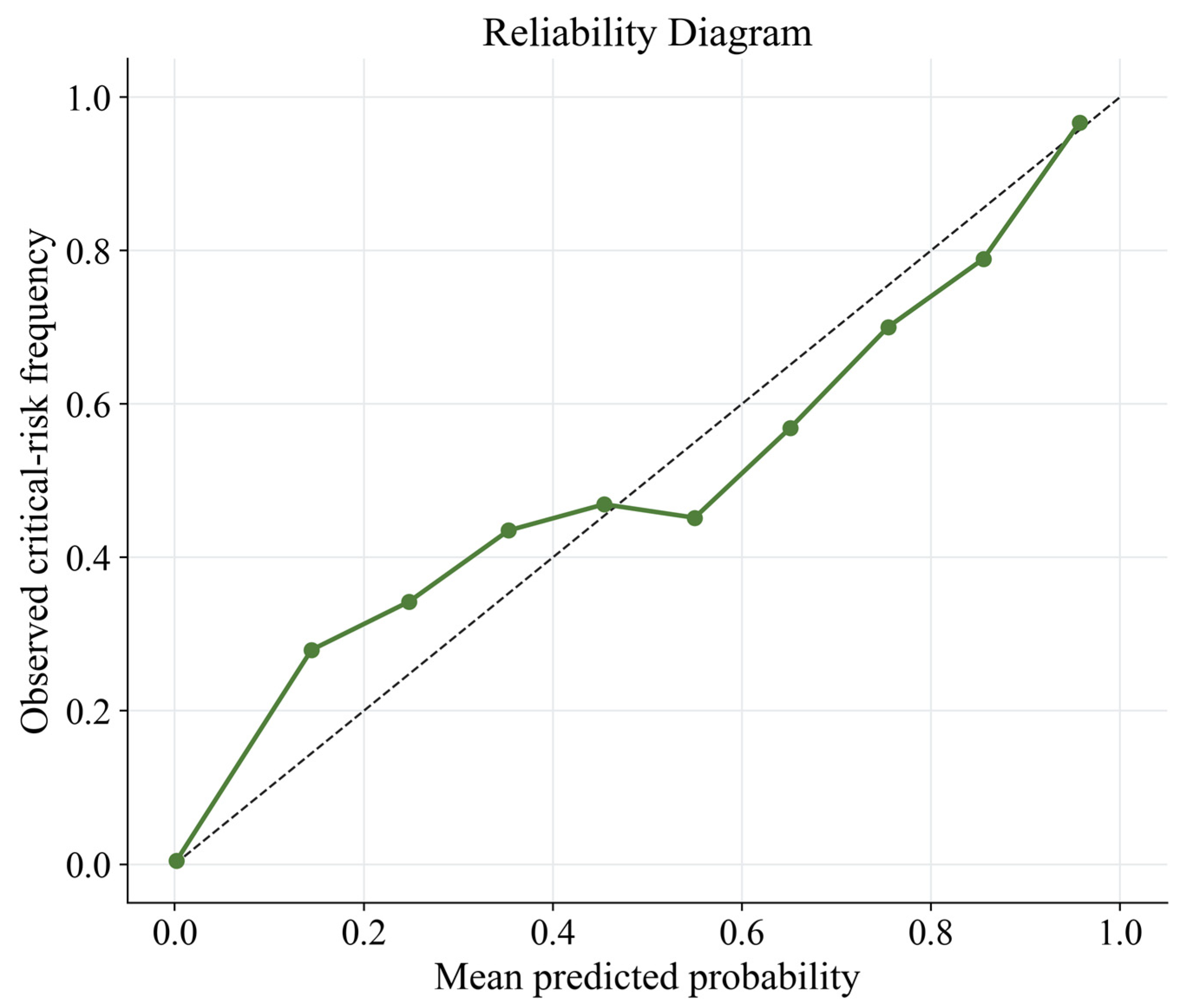
The reliability diagram confirms that the calibrated probabilities are not merely classifier scores but carry interpretable risk information. In the low-probability range, predicted and observed risk frequencies remain close to zero, while high predicted risk levels correspond to high observed overload-risk frequencies. Moderate deviations in the middle probability range indicate local underestimation or overestimation, which is also reflected by the ECE metric.

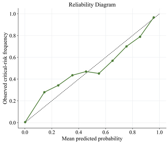
Table 11 compares the interval forecasting quality of B-TGPRF with the Quantile Gradient Boosting conformal baseline using pinball loss, empirical coverage, mean interval width, and uncertainty–error correlation. Figure 4 shows the reliability diagram of the calibrated overload-risk probabilities on the strict external-like test. The dotted diagonal line represents perfect calibration, while the green curve shows the observed critical-risk frequency for different predicted-probability bins.

Table 11. Strict external test: interval forecasting quality.

Model	Group	Pinball Loss	Coverage	Mean Interval Width	Uncertainty–Error Correlation
Quantile Gradient Boosting conformal	Boosting	0.1710	0.9959	6.7987	-
B-TGPRF	Proposed	0.0678	0.8494	1.3891	−0.0208

Figure 4. Reliability diagram of calibrated overload-risk probabilities on the strict external-like test. The dotted diagonal line indicates perfect calibration, and the green curve shows the observed critical-risk frequency across predicted-probability bins.

Supplementary Table S4 provides the full validation and external-like interval forecasting comparison. Across both splits, B-TGPRF achieved substantially lower pinball loss and narrower intervals than the Quantile Gradient Boosting conformal baseline, while the latter achieved higher empirical coverage through much wider prediction intervals.

The conformal boosting baseline achieved higher empirical coverage, but its intervals were substantially wider. B-TGPRF provided a narrower and more informative interval, with lower pinball loss, making it more useful for near-threshold overload diagnostics. This result illustrates the difference between maximum coverage and practical interval informativeness.

Table 12 extends the interval evaluation by adding approximate CRPS, Winkler score, prediction interval coverage probability, mean prediction interval width, and sharpness. These metrics provide a more complete view of the trade-off between interval accuracy, coverage, and compactness.

Table 12. Additional probabilistic interval assessment on the strict external-like test.

Model	Approx. CRPS ↓	Winkler Score ↓	PICP ↑	MPIW ↓	Sharpness ↓
B-TGPRF	0.2122	2.7139	0.8492	1.3891	1.3891
Quantile Gradient Boosting conformal	0.3730	6.8409	0.9959	6.7987	6.7987

Note: ↑ denotes metrics for which higher values are preferable, whereas ↓ denotes metrics for which lower values are preferable.

The additional interval metrics confirm a coverage–width trade-off. The Quantile Gradient Boosting conformal baseline achieved higher empirical coverage but produced much wider intervals. B-TGPRF produced substantially narrower and sharper intervals with a lower approximate CRPS and Winkler score, but its empirical coverage was lower. Therefore, B-TGPRF should be interpreted as a compact diagnostic interval model rather than as a conservative high-coverage safety envelope.

4.4. Ablation and Robustness Analysis

The ablation results reveal that the complete model is not designed to maximize one isolated metric. Instead, it balances forecasting accuracy, risk calibration, interval compactness, and conservative risk decisions. Temporal-only variants were strong in some metrics, but removing calibration substantially degraded ECE and removing residual correction worsened the forecasting and interval quality.

Table 13 reports the selected ablation results on the strict external-like test. The table compares the complete B-TGPRF configuration with simplified variants in which graph context, residual correction, or calibration is removed.

Table 13. Strict external test: selected ablation results.

Variant	Removed Component	MAE	Macro-F1	Brier Score	ECE	Mean Width
Temporal-only representation	Graph and regime context	0.3614	0.9123	0.0131	0.0038	1.5650
Complete B-TGPRF	No component removed	0.3650	0.8960	0.0147	0.0064	1.3891
Without residual correction	Residual correction	0.3690	0.9040	0.0141	0.0055	1.8160
Without graph features	Graph-neighborhood representation	0.3788	0.9047	0.0142	0.0055	1.5339
Without calibration	Probability calibration	0.3795	0.8966	0.0257	0.0786	1.5359

The ablation results indicate that individual simplified variants may outperform the complete framework on isolated metrics. In particular, the temporal-only variant is very strong for short-horizon point forecasting and several classification indicators. However, the complete B-TGPRF is not optimized to dominate every single metric independently. Its objective is to provide a balanced multi-output decision-support profile that combines competitive line-flow forecasting, calibrated risk probability, compact interval uncertainty, graph-aware interpretability, and conservative false-positive behavior. Therefore, the ablation study should be interpreted in terms of component-specific trade-offs rather than simple monotonic improvement from adding each module.

To make the component-level contribution more explicit, the ablation results were additionally interpreted as metric changes relative to the complete B-TGPRF configuration on the strict external-like test. This analysis shows that different components contribute to different operational dimensions. The temporal representation is the strongest source of point-forecasting accuracy, probability calibration is the most important component for probability reliability, residual correction improves local forecasting and interval behavior, and graph, topology, and operating-regime descriptors provide additional electrical and operational context. Table 14 reports the quantitative contribution of each B-TGPRF component on the strict external-like test. The table shows changes in MAE, Macro-F1, Recall, ECE, and pinball loss relative to the complete B-TGPRF configuration.

Table 14. Quantitative contribution of B-TGPRF components on the strict external-like test.

Component/Variant	ΔMAE vs. Full	ΔMacro-F1 vs. Full	ΔRecall vs. Full	ΔECE vs. Full	ΔPinball vs. Full	Interpretation
Temporal-only	−0.0031	+0.0163	+0.1029	−0.0026	−0.0031	Strongest contribution to point forecasting
Without graph features	+0.0136	+0.0088	+0.1066	−0.0009	+0.0010	Graph context improves MAE but changes recall/FPR trade-off
Without topology features	+0.0142	+0.0102	+0.0977	−0.0014	+0.0010	Topology supports forecasting accuracy
Without regime features	+0.0143	+0.0145	+0.0940	−0.0022	+0.0010	Regime features support forecasting
Without Bayesian layer	+0.0138	+0.0114	+0.0878	−0.0005	+0.0009	Bayesian layer contributes to risk fusion
Without calibration	+0.0138	+0.0006	+0.0522	+0.0722	+0.0009	Calibration is critical for probability reliability
Without residual correction	+0.0037	+0.0080	+0.0921	−0.0009	+0.0001	Residual correction refines forecasting
Zero-width interval	0.0000	0.0000	0.0000	0.0000	+0.1148	Interval estimation is necessary for uncertainty

The ablation study shows that complex graph, topology, and operating-regime features are not universally beneficial for every metric. In particular, the temporal-only representation achieves slightly better MAE, Macro-F1, Recall, and ECE than the complete B-TGPRF on the 1 h external-like test. This indicates that recent temporal line-flow dynamics carry the dominant predictive signal for short-horizon forecasting and risk detection. Therefore, the role of complex features should be interpreted more narrowly: they provide topology-aware and regime-aware context, support diagnostic interpretation, and contribute to a multi-output probabilistic risk framework, but they do not guarantee monotonic improvement in every numerical metric. The full B-TGPRF should therefore be interpreted as a balanced decision-support configuration rather than as the best variant for each isolated metric.

The detailed ablation of the calibration and interval components is reported in Supplementary Table S5. The removal of the calibration layer substantially worsened ECE and Brier Score, confirming that calibration is not a cosmetic post-processing step but a necessary component for aligning predicted risk probabilities with observed events.

The ablation results should not be interpreted as evidence that the complete model must dominate every individual metric. Temporal-only variants are strong for short-horizon point forecasting, but the complete B-TGPRF is designed as a multi-output probabilistic system. Its value lies in combining competitive forecasting accuracy, calibrated risk probability, compact interval prediction, uncertainty diagnostics, and conservative false-positive behavior.

Threshold sensitivity showed that q95 was the best-balanced risk threshold in terms of calibration. Horizon sensitivity indicated that the 1 h horizon was the most reliable, whereas 6 h and 24 h horizons require additional optimization and potentially richer temporal context.

Table 15 reports the sensitivity of B-TGPRF to different risk thresholds and forecast horizons. The threshold comparison evaluates q90, q95, and q99, while the horizon comparison shows how performance changes from 1 h to 6 h and 24 h forecasting.

Table 15. Sensitivity to risk thresholds and forecast horizons.

Analysis	Setting	MAE	Macro-F1	Balanced Accuracy	Brier Score	ECE
Threshold	q90	-	0.9488	-	0.0438	0.0498
Threshold	q95	-	0.9372	-	0.0147	0.0064
Threshold	q99	-	0.8923	-	0.0320	0.0374
Horizon	1 h	0.3650	0.8960	0.8747	0.0147	0.0064
Horizon	6 h	3.6087	0.5615	0.5941	0.0554	0.0609
Horizon	24 h	3.0398	0.6564	0.6802	0.0589	0.1065

The degradation at the 6 h and 24 h horizons is substantial and should be interpreted as a limitation of the present B-TGPRF configuration. The model is most reliable for 1 h operational forecasting because short-horizon line-flow dynamics contain strong temporal persistence and recent lag, rolling, and ramp features remain highly informative. At longer horizons, this direct autoregressive relationship weakens, while accumulated changes in load, generation, redispatch-like effects, and regime transitions become more important. The current architecture does not include horizon-specific exogenous forecasts of future load, renewable generation, dispatch schedules, or contingency plans. Therefore, the 6 h and 24 h results are reported transparently as diagnostic long-horizon limitations rather than as deployment-ready long-horizon performance. Future work should use horizon-specific encoders, longer lookback windows, sequence-to-sequence multi-horizon learning, richer exogenous variables, and separate multi-horizon calibration.

The q95 threshold was selected as the main operating threshold because it provides a compromise between event frequency, strictness of the overload-risk definition, and probability calibration. The q90 threshold creates a broader warning class but weakens calibration, whereas q99 makes the positive class rarer and increases the difficulty of stable risk learning. Therefore, q95 is used as the primary operational risk threshold because it is strict enough to represent near-critical operation while still providing a sufficient number of positive events for training and calibration.

4.5. Safety-Critical Subgroup Evaluation

Table 16 reports the safety-critical subgroup evaluation of B-TGPRF on the strict external-like test. The model was assessed under high-load, high-ramp, low-margin, stress, near-threshold, central-line, and peripheral-line conditions to determine whether its performance remains stable beyond average global metrics.

Table 16. Safety-critical subgroup evaluation of B-TGPRF on the strict external-like test.

Subgroup	MAE ↓	Macro-F1 ↑	Recall ↑	FNR ↓	Brier Score ↓	ECE ↓	Coverage ↑
High-load periods	0.4206	0.8750	0.6400	0.3600	0.0186	0.0182	0.8078
High-ramp periods	0.3572	0.8958	0.7552	0.2448	0.0139	0.0060	0.8574
Low-margin periods	0.2915	0.8757	0.7578	0.2422	0.0596	0.0262	0.9007
Stress periods	0.3491	0.8710	0.6935	0.3065	0.0477	0.0294	0.8600
Near-threshold periods	0.2530	0.8256	0.7014	0.2986	0.1042	0.0464	0.9169
Central lines	0.3529	0.9141	0.7961	0.2039	0.0119	0.0037	0.8559
Peripheral lines	0.3792	0.8745	0.7110	0.2890	0.0180	0.0099	0.8418

Note: ↑ denotes metrics for which higher values are preferable, whereas ↓ denotes metrics for which lower values are preferable.

The subgroup results show that B-TGPRF is more reliable for central lines and high-ramp periods, while high-load, stress, and near-threshold regimes remain more challenging. In particular, the false-negative rate increases in high-load and stress periods, indicating that safety-critical deployment would require recall-oriented threshold tuning and additional validation under contingency-like and rare-event scenarios.

To further address safety-critical operating conditions, additional scenario-proxy checks were conducted on the strict external-like test. These checks included contingency-like proxy conditions, defined by the top 1% neighbor-stress and line-loading cases, as well as additional regime-oriented subgroup checks. These proxy groups do not replace full contingency simulation or real renewable-intermittency testing, but they provide a stricter stress-oriented diagnostic evaluation within the available benchmark. Table 17 reports additional safety-critical scenario-proxy metrics for B-TGPRF, including overall performance, high-load and high-ramp periods, central and peripheral lines, and the contingency-like proxy subgroup.

Table 17. Additional safety-critical scenario-proxy metrics for B-TGPRF.

Subgroup	Rows	Positive Rate	Recall	FNR	Precision	Macro-F1	Brier	ECE
Overall	59,999	0.0543	0.7568	0.2432	0.8544	0.8960	0.0147	0.0064
High-load	14,438	0.0650	0.6400	0.3600	0.9465	0.8750	0.0186	0.0183
High-ramp	15,128	0.0513	0.7552	0.2448	0.8542	0.8958	0.0139	0.0060
Central lines	32,350	0.0541	0.7961	0.2039	0.8823	0.9141	0.0119	0.0037
Peripheral lines	27,649	0.0544	0.7110	0.2890	0.8206	0.8745	0.0180	0.0099
Contingency-like proxy	600	0.3083	0.9081	0.0919	0.9545	0.9505	—	—

The results show that the contingency-like proxy subgroup has a much higher positive-risk rate than the overall external-like test and that B-TGPRF achieves stronger recall and Macro-F1 under this proxy condition. However, because this subgroup is derived from benchmark stress indicators rather than from a full N–k contingency simulation, it should be interpreted as a diagnostic stress check rather than as complete contingency validation.

4.6. Runtime, Memory, and Scalability Assessment

Because B-TGPRF consists of several sequential processing stages, runtime, memory use, and scalability were additionally measured. In the saved final configuration, B-TGPRF used 100 selected lines, 1,572,300 training rows, and 871,200 external-test rows. The training time was 4.144 s, the inference time was approximately 0.0161 s per 10,000 observations, and peak RAM use was approximately 3457 MB. A compact scaling rerun was also conducted for 20 and 100 selected lines under the same sample budget. The training time was 0.9883 s and 0.9889 s, respectively, while the inference time per 10,000 observations remained below 0.017 s. These results indicate that the inference overhead of the tabular graph-temporal representation remains low. A 200-line scaling experiment was not artificially created because the current selected-line dataset contains 100 lines; therefore, no fabricated 200-line result is reported.

Table 18 indicates that B-TGPRF has low inference latency under the tabular graph-temporal representation. The compact scaling experiment also shows that increasing the selected-line count from 20 to 100 did not materially increase inference time under the same sample budget, although larger real EMS deployments would still require additional production-grade testing.

Table 18. Runtime, memory, and scalability assessment.

Configuration	Lines	Train Rows	Test Rows	Train Time, s	Inference per 10 k, s	Peak RAM, MB
B-TGPRF final external	100	1,572,300	871,200	4.144	0.0161	3457
Compact HGB scaling	20	30,000	8000	0.9883	0.0167	2592
Compact HGB scaling	100	30,000	8000	0.9889	0.0158	3232

These measurements suggest that the proposed workflow can be executed with low inference overhead in the present benchmark setting. Nevertheless, the scalability results should be interpreted as benchmark-level evidence, and production EMS deployment would require additional testing under larger networks, streaming data, and real communication constraints.

The runtime values were obtained on the authors’ experimental computing environment; hardware-specific latency may vary across CPU/GPU configurations and production EMS infrastructure.

4.7. Robustness Under Realistic Data-Quality Disturbances

To approximate realistic SCADA/PMU data-quality disturbances, an additional robustness analysis was conducted for the B-TGPRF risk layer. The tested disturbance scenarios included missing values at different levels, Gaussian noise equal to 5% of feature standard deviation, communication delays of 1 h and 2 h, line-flow sensor dropout, and topology feature dropout. The objective of this analysis was not to fully reproduce operational EMS conditions, but to evaluate the sensitivity of the proposed framework to realistic measurement imperfections. Table 19 reports the robustness analysis for the B-TGPRF risk layer under realistic data-quality disturbances, including missing values, Gaussian noise, communication delay, line-flow sensor dropout, and topology feature dropout.

Table 19. Robustness analysis for the B-TGPRF risk layer.

Scenario	Macro-F1	Recall	FNR	Brier	ECE
Clean	0.8975	0.7596	0.2404	0.0154	0.0071
Missing 5%	0.8989	0.7486	0.2514	0.0154	0.0075
Missing 20%	0.8774	0.6716	0.3284	0.0158	0.0093
Gaussian noise 5%	0.8404	0.5486	0.4514	0.0172	0.0170
Delay 1 h	0.8804	0.6716	0.3284	0.0158	0.0097
Delay 2 h	0.8737	0.6569	0.3431	0.0159	0.0095
Sensor dropout line-flow	0.8822	0.6752	0.3248	0.0160	0.0104
Topology dropout 5%	0.8971	0.7560	0.2440	0.0154	0.0073

The robustness results show that B-TGPRF remains relatively stable under moderate missingness and topology feature dropout, but it is more sensitive to measurement noise, delayed observations, and line-flow sensor dropout. In particular, Gaussian noise and communication delay reduce recall and increase the false-negative rate. This finding is important for safety-critical deployment because missed overload-risk events are usually more costly than false alarms. Therefore, real EMS deployment would require missing-value monitoring, delay-aware input flags, sensor-quality checks, topology-version tracking, and periodic recalibration.

5. Discussion

The results support the view that overload-risk forecasting should be treated as a multi-output probabilistic task rather than as a simple point-forecasting or classification problem. B-TGPRF is particularly strong in forecasting future line flow and in providing calibrated risk probabilities and compact prediction intervals.

The practical role of B-TGPRF is to support monitoring and early warning rather than to replace physical power-flow calculations, contingency analysis, or operator safety procedures. The model provides a probabilistic risk signal, a future line-flow forecast, an uncertainty interval, and diagnostic information about prediction confidence. These outputs should be used as analytical support for prioritizing vulnerable lines and near-threshold regimes, while final operational decisions should remain grounded in engineering constraints and operator procedures.

The comparison also shows that boosting models remain highly competitive for pure risk-class detection. This finding should not be hidden. B-TGPRF does not dominate every classification metric. Instead, it offers a different operational profile, prioritizing calibrated probability, compact uncertainty intervals, and low false-positive risk-signaling. In operational settings, this profile can be valuable because excessive false alarms may reduce operator trust in decision-support tools.

Subgroup analysis further indicates that B-TGPRF does not behave uniformly across all operating regimes. The model is more stable for central lines and high-ramp periods, while high-risk and near-threshold regimes remain more difficult due to class rarity and boundary ambiguity. This result supports the need to evaluate overload-risk models not only by global metrics but also by operating-regime and topological subgroups.

The ablation analysis confirms that the architecture is meaningful. The temporal branch carries the strongest predictive information, but calibration, residual correction, graph-context features, and uncertainty modeling each contribute to different dimensions of reliability. This makes the proposed model more suitable as a decision-support component than as a single-purpose classifier.

From a methodological perspective, the study demonstrates that carefully engineered graph-temporal features can remain highly competitive with compact deep architectures. This does not imply that full graph neural networks or Transformers are ineffective; rather, it shows that, for this benchmark and protocol, a hybrid probabilistic architecture with strong leakage control and calibrated outputs provides a favorable balance of accuracy and interpretability.

Limitations

This study uses one open synthetic benchmark dataset rather than operational data from a real transmission-system operator. The external test is an external-like scenario-group evaluation within the same benchmark, not a completely independent field dataset. Therefore, the reported results demonstrate methodological effectiveness and scenario-level robustness under controlled benchmark conditions, but they should not be interpreted as direct field validation. Future work should extend the evaluation to multiple years, additional scenario groups, stress-test simulations, and real SCADA/PMU data when such data become available.

6. Conclusions

This article presented B-TGPRF, a Bayesian temporal graph probabilistic model for calibrated overload-risk forecasting in power transmission grids. The model combines temporal dynamics, graph-topological information, operating-regime features, residual correction, Bayesian risk estimation, probability calibration, conformal interval construction, and diagnostic uncertainty. A leakage-controlled data preparation pipeline was built from an open benchmark dataset, and the model was evaluated using chronological train, validation, test, and strict external-like scenario partitions.

The results demonstrate that B-TGPRF provides accurate line-flow forecasts, calibrated risk probabilities, compact prediction intervals, and conservative false-alarm behavior. On the strict external-like scenario test, it achieved MAE = 0.3650, RMSE = 0.5478, R² = 0.9962, Brier Score = 0.0147, and ECE = 0.0064. Although boosting models remained stronger for some pure classification metrics, B-TGPRF achieved the strongest overall balance between forecasting accuracy, calibrated risk estimation, compact interval prediction, and operational interpretability. A key limitation is that the external-like scenario test is derived from the same synthetic benchmark family and should not be interpreted as independent field validation on real transmission-system operator data. Therefore, the present results demonstrate controlled benchmark reproducibility and scenario-level robustness rather than direct operational readiness. Future work should validate the framework on multi-year data, additional scenario groups, stress-test simulations, and real SCADA/PMU measurements when such data become available. Future work will focus on multi-year validation, additional operating scenarios, improved long-horizon forecasting, and testing on real transmission-grid operational datasets.

References

- Kaur, D.; Islam, S.N.; Mahmud, M.A.; Haque, M.E.; Dong, Z.Y. Energy forecasting in smart grid systems: Recent advancements in probabilistic deep learning. IET Gener. Transm. Distrib. 2022, 16, 4461–4479. [Google Scholar] [CrossRef] [Scilit]
- Khajeh, H.; Laaksonen, H. Applications of probabilistic forecasting in smart grids: A review. Appl. Sci. 2022, 12, 1823. [Google Scholar] [CrossRef] [Scilit]
- Tomin, N.V.; Kurbatsky, V.G.; Sidorov, D.N.; Zhukov, A.V. Machine learning techniques for power system security assessment. IFAC-PapersOnLine 2016, 49, 445–450. [Google Scholar] [CrossRef] [Scilit]
- Alimi, O.A.; Ouahada, K.; Abu-Mahfouz, A.M. A review of machine learning approaches to power system security and stability. IEEE Access 2020, 8, 113512–113531. [Google Scholar] [CrossRef] [Scilit]
- Khodayar, M.; Regan, J. Deep neural networks in power systems: A review. Energies 2023, 16, 4773. [Google Scholar] [CrossRef] [Scilit]
- Chen, T.; Guestrin, C. XGBoost: A scalable tree boosting system. In Proceedings of the 22nd ACM SIGKDD International Conference on Knowledge Discovery and Data Mining, San Francisco, CA, USA, 13–17 August 2016; pp. 785–794. [Google Scholar] [CrossRef] [Scilit]
- Ke, G.; Meng, Q.; Finley, T.; Wang, T.; Chen, W.; Ma, W.; Ye, Q.; Liu, T.Y. LightGBM: A highly efficient gradient boosting decision tree. In Proceedings of the Advances in Neural Information Processing Systems, Long Beach, CA, USA, 4–9 December 2017; Available online: https://papers.nips.cc/paper_files/paper/2017/hash/6449f44a102fde848669bdd9eb6b76fa-Abstract.html (accessed on 8 June 2026).
- Breiman, L. Random forests. Mach. Learn. 2001, 45, 5–32. [Google Scholar] [CrossRef] [Scilit]
- Geurts, P.; Ernst, D.; Wehenkel, L. Extremely randomized trees. Mach. Learn. 2006, 63, 3–42. [Google Scholar] [CrossRef] [Scilit]
- Liao, W.; Bak-Jensen, B.; Pillai, J.R.; Wang, Y.; Wang, Y. A review of graph neural networks and their applications in power systems. J. Mod. Power Syst. Clean Energy 2022, 10, 345–360. [Google Scholar] [CrossRef] [Scilit]
- Yaniv, A.; Kumar, P.; Beck, Y. Towards adoption of GNNs for power flow applications in distribution systems. Electr. Power Syst. Res. 2023, 216, 109005. [Google Scholar] [CrossRef] [Scilit]
- Alvarez, D.L.; Gaha, M.; Prévost, J.; Côté, A.; Abdul-Nour, G.; Meango, T.J.-M. N–k static security assessment for power transmission system planning using machine learning. Energies 2024, 17, 292. [Google Scholar] [CrossRef] [Scilit]
- De Caro, F.; Giannuzzi, G.M.; Pisani, C.; Iuliano, S.; Vaccaro, A. The role of data-driven methods in power system security assessment from aggregated grid data. Front. Smart Grids 2024, 3, 1385367. [Google Scholar] [CrossRef] [Scilit]
- Varbella, A.; Amara, K.; Gjorgiev, B.; El-Assady, M.; Sansavini, G. PowerGraph: A power grid benchmark dataset for graph neural networks. Adv. Neural Inf. Process. Syst. 2024, 37, 110784–110804. [Google Scholar] [CrossRef] [Scilit]
- Ghamizi, S.; Bojchevski, A.; Ma, A.; Cao, J. SafePowerGraph: Safety-aware evaluation of graph neural networks for transmission power grids. arXiv 2024. [Google Scholar] [CrossRef] [Scilit]
- Kipf, T.N.; Welling, M. Semi-supervised classification with graph convolutional networks. In Proceedings of the International Conference on Learning Representations, Toulon, France, 24–26 April 2017. [Google Scholar] [CrossRef] [Scilit]
- Veličković, P.; Cucurull, G.; Casanova, A.; Romero, A.; Liò, P.; Bengio, Y. Graph attention networks. In Proceedings of the International Conference on Learning Representations, Vancouver, BC, Canada, 30 April–3 May 2018. [Google Scholar] [CrossRef] [Scilit]
- Hamilton, W.L.; Ying, R.; Leskovec, J. Inductive representation learning on large graphs. In Proceedings of the Advances in Neural Information Processing Systems, Long Beach, CA, USA, 4–9 December 2017. [Google Scholar] [CrossRef] [Scilit]
- Xu, K.; Hu, W.; Leskovec, J.; Jegelka, S. How powerful are graph neural networks? In Proceedings of the International Conference on Learning Representations, New Orleans, LA, USA, 6–9 May 2019. [Google Scholar] [CrossRef] [Scilit]
- Zhou, J.; Cui, G.; Hu, S.; Zhang, Z.; Yang, C.; Liu, Z.; Wang, L.; Li, C.; Sun, M. Graph neural networks: A review of methods and applications. AI Open 2020, 1, 57–81. [Google Scholar] [CrossRef] [Scilit]
- Yu, B.; Yin, H.; Zhu, Z. Spatio-temporal graph convolutional networks: A deep learning framework for traffic forecasting. In Proceedings of the 27th International Joint Conference on Artificial Intelligence, Stockholm, Sweden, 13–19 July 2018; pp. 3634–3640. [Google Scholar] [CrossRef] [Scilit] [PubMed]
- Wu, Z.; Pan, S.; Long, G.; Jiang, J.; Zhang, C. Graph WaveNet for deep spatial-temporal graph modeling. In Proceedings of the 28th International Joint Conference on Artificial Intelligence, Macao, China, 10–16 August 2019; pp. 1907–1913. [Google Scholar] [CrossRef] [Scilit] [PubMed]
- Vaswani, A.; Shazeer, N.; Parmar, N.; Uszkoreit, J.; Jones, L.; Gomez, A.N.; Kaiser, L.; Polosukhin, I. Attention is all you need. In Proceedings of the Advances in Neural Information Processing Systems, Long Beach, CA, USA, 4–9 December 2017. [Google Scholar] [CrossRef] [Scilit]
- Hochreiter, S.; Schmidhuber, J. Long short-term memory. Neural Comput. 1997, 9, 1735–1780. [Google Scholar] [CrossRef] [Scilit] [PubMed]
- Cho, K.; van Merriënboer, B.; Gulcehre, C.; Bahdanau, D.; Bougares, F.; Schwenk, H.; Bengio, Y. Learning phrase representations using RNN encoder-decoder for statistical machine translation. In Proceedings of the 2014 Conference on Empirical Methods in Natural Language Processing, Doha, Qatar, 25–29 October 2014; pp. 1724–1734. [Google Scholar] [CrossRef] [Scilit]
- Bai, S.; Kolter, J.Z.; Koltun, V. An empirical evaluation of generic convolutional and recurrent networks for sequence modeling. arXiv 2018. [Google Scholar] [CrossRef] [Scilit]
- Salinas, D.; Flunkert, V.; Gasthaus, J.; Januschowski, T. DeepAR: Probabilistic forecasting with autoregressive recurrent networks. Int. J. Forecast. 2020, 36, 1181–1191. [Google Scholar] [CrossRef] [Scilit]
- Lim, B.; Arık, S.Ö.; Loeff, N.; Pfister, T. Temporal Fusion Transformers for interpretable multi-horizon time series forecasting. Int. J. Forecast. 2021, 37, 1748–1764. [Google Scholar] [CrossRef] [Scilit]
- Nie, Y.; Nguyen, N.H.; Sinthong, P.; Kalagnanam, J. A time series is worth 64 words: Long-term forecasting with Transformers. In Proceedings of the International Conference on Learning Representations, Kigali, Rwanda, 1–5 May 2023. [Google Scholar] [CrossRef] [Scilit]
- Zhao, J.; Chu, F.; Xie, L.; Che, Y.; Wu, Y.; Burke, A.F. A survey of transformer networks for time series forecasting. Comput. Sci. Rev. 2026, 60, 100883. [Google Scholar] [CrossRef] [Scilit]
- Kim, J.; Kim, H.; Kim, H.G.; Lee, D.; Yoon, S. A comprehensive survey of deep learning for time series forecasting: Architectural diversity and open challenges. Artif. Intell. Rev. 2025, 58, 216. [Google Scholar] [CrossRef] [Scilit]
- Blundell, C.; Cornebise, J.; Kavukcuoglu, K.; Wierstra, D. Weight uncertainty in neural networks. In Proceedings of the 32nd International Conference on Machine Learning, Lille, France, 6–11 July 2015; Volume 37, pp. 1613–1622. [Google Scholar] [CrossRef] [Scilit]
- Gal, Y.; Ghahramani, Z. Dropout as a Bayesian approximation: Representing model uncertainty in deep learning. In Proceedings of the 33rd International Conference on Machine Learning, New York, NY, USA, 19–24 June 2016; Volume 48, pp. 1050–1059. [Google Scholar] [CrossRef] [Scilit]
- Lakshminarayanan, B.; Pritzel, A.; Blundell, C. Simple and scalable predictive uncertainty estimation using deep ensembles. In Proceedings of the Advances in Neural Information Processing Systems, Long Beach, CA, USA, 4–9 December 2017. [Google Scholar] [CrossRef] [Scilit]
- Guo, C.; Pleiss, G.; Sun, Y.; Weinberger, K.Q. On calibration of modern neural networks. In Proceedings of the 34th International Conference on Machine Learning, Sydney, Australia, 6–11 August 2017. [Google Scholar] [CrossRef] [Scilit]
- Angelopoulos, A.N.; Bates, S. Conformal prediction: A gentle introduction. Found. Trends Mach. Learn. 2023, 16, 494–591. [Google Scholar] [CrossRef] [Scilit]
- Gneiting, T.; Raftery, A.E. Strictly proper scoring rules, prediction, and estimation. J. Am. Stat. Assoc. 2007, 102, 359–378. [Google Scholar] [CrossRef] [Scilit]
- O’Connor, C.; Bahloul, M.; Rossi, R.; Prestwich, S.; Visentin, A. Conformal prediction for electricity price forecasting in the day-ahead and real-time balancing market. Energy AI 2025, 21, 100571. [Google Scholar] [CrossRef] [Scilit]
- Borrotti, M. Quantifying uncertainty with conformal prediction for heating and cooling load forecasting in building performance simulation. Energies 2024, 17, 4348. [Google Scholar] [CrossRef] [Scilit]
- Jiang, Y.; Zhu, C.; Zou, F.; Zhang, L.; Yu, X.; Pan, C.; Liao, S. Stepwise conformal prediction for multi-step net load forecasting in microgrids under renewable energy variability. Energies 2026, 19, 2297. [Google Scholar] [CrossRef] [Scilit]
- Kuleshov, V.; Fenner, N.; Ermon, S. Accurate uncertainties for deep learning using calibrated regression. In Proceedings of the 35th International Conference on Machine Learning, Stockholm, Sweden, 10–15 July 2018; Volume 80, pp. 2796–2804. Available online: https://proceedings.mlr.press/v80/kuleshov18a.html (accessed on 8 June 2026).
- Zadrozny, B.; Elkan, C. Transforming classifier scores into accurate multiclass probability estimates. In Proceedings of the 8th ACM SIGKDD International Conference on Knowledge Discovery and Data Mining, Edmonton, AB, Canada, 23–26 July 2002; pp. 694–699. [Google Scholar] [CrossRef] [Scilit]
- Niculescu-Mizil, A.; Caruana, R. Predicting good probabilities with supervised learning. In Proceedings of the 22nd International Conference on Machine Learning, Bonn, Germany, 7–11 August 2005; pp. 625–632. [Google Scholar] [CrossRef] [Scilit]
- Taganova, G.; Tussupov, J.; Abdildayeva, A.; Kaldarova, M.; Kazi, A.; Simpson, R.C.; Zakirova, A.; Nurbekov, B. HST–MB–CREH: A Hybrid Spatio-Temporal Transformer with Multi-Branch CNN/RNN for Rare-Event-Aware PV Power Forecasting. Algorithms 2026, 19, 94. [Google Scholar] [CrossRef] [Scilit]
- Taganova, G.; Zakirova, A.; Abdildayeva, A.; Nurbekov, B.; Akhayeva, Z.; Azykanov, T. Sub-Hourly Multi-Horizon Quantile Forecasting of Photovoltaic Power Using Meteorological Data and a HybridCNN–STTransformer. Algorithms 2026, 19, 123. [Google Scholar] [CrossRef] [Scilit]
- Gillioz, M.; Dubuis, G.; Jacquod, P. A large synthetic dataset for machine learning applications in power transmission grids. Sci. Data 2025, 12, 168. [Google Scholar] [CrossRef] [Scilit] [PubMed]
- Gillioz, M.; Dubuis, G.; Jacquod, P. A large synthetic dataset for machine learning applications in power transmission grids. Zenodo 2024. [Google Scholar] [CrossRef]
Disclaimer/Publisher’s Note: The statements, opinions and data contained in all publications are solely those of the individual author(s) and contributor(s) and not of MDPI and/or the editor(s). MDPI and/or the editor(s) disclaim responsibility for any injury to people or property resulting from any ideas, methods, instructions or products referred to in the content. |
© 2026 by the authors. Licensee MDPI, Basel, Switzerland. This article is an open access article distributed under the terms and conditions of the Creative Commons Attribution (CC BY) license.