


Abstract
The Colonel Blotto game, formulated by Émile Borel, involves players allocating limited resources to multiple “battlefields” simultaneously, with the winner being the one who allocates more resources to each battlefield. Computation of the Nash equilibrium, including of two-person, zero-sum, mixed strategy Colonel Blotto games have encountered issues of scalability and complexity owing to their PPAD completeness. This paper proposes an algorithm that computes the same value as the Nash equilibrium but cannot be characterized by the Fixed-Point Theorems of Tarski, Kakutani and Brouwer. The reduced complexity of the proposed algorithm is based on dispensing with the need for computing both players’ Nash strategies in Colonel Blotto games. The same algorithm can, therefore, be extended to all two-person, zero-sum games to compute the value of the Nash equilibrium. The theoretical superiority of the proposed algorithm over both LP solvers and another method that computes the same value of the game as its Nash equilibrium by a random assignment of probabilities to the active strategy set of the defending player, is also proposed.
1. Introduction
A Colonel Blotto game is a two-person zero-sum game in which the players are required to simultaneously distribute limited resources over more than one object. The player allocating the greater resource to the object wins it [1,2,3,4,5,6,7,8,9]. The game was formulated by the French mathematician Emile Borel in 1921 [10]. It was published by Borel and Jean Ville as an application of the Theory of Probability and of the Game of Chance in 1938 [11]. Popularized by Operations Research scholars after the Second World War, Borel’s game became and remains a classic in the literature of Game Theory under the name of the Colonel Blotto Game.
Strategic resource allocation using the Colonel Blotto game has applications not only in military settings, but also in politics, network security, hiring decisions and even competition for social media attention. Its pre-eminent use, however, has been in the field of security and conflict, involving allocation of defense resources to a certain number of ‘battlefields’ that is the object of contest between adversaries.
2. Literature Review and Motivation
Chen, Deng and Teng [12], Daskalakis, Goldberg and Papadimitriou [9] showed that computing a Nash equilibrium in a Colonel Blotto game was PPAD complete owing to the CB game’s structural properties of non-convexity and non-linearity. They [9] also proved the reduction of the Brouwer Fixed Point Theorem to the polynomial parity argument for directed graphs (PPAD) class and then showed the reduction of Nash to Brouwer to prove that Nash was in PPAD. Nash in his 1950 proof had himself relied on both the Brouwer and Kakutani Fixed Point Theorems to show that a mixed strategy Nash Equilibrium existed for finite games.
We show, however, in this paper, that, using our proposed algorithm, it is possible to compute the Nash Equilibrium value of a two person, zero sum Colonel Blotto Game even while deviating from the framework and requirements of the Kakutani Fixed Point Theorem and, by extension of discrete strategies spaces to continuous strategies spaces, also while deviating from the framework and requirements of the Brouwer Fixed Point Theorem.
Roberto Ricci used Tarski’s Fixed-Point Theorem to prove the existence of pure strategy Nash Equilibria for two player games with possible discontinuous payoff functions defined on compact real intervals.
We prove that the Nash Equilibrium value of the two persons, zero sum Colonel Blotto Game can be computed even by deviating from the framework of the Tarski Fixed Point Theorem.
Ahmadinejad et al. [13] discussed the scalability issues in computing Nash equilibria for large Colonel Blotto games. They proposed a heuristic approach to reduce the game’s computational complexity. The authors suggested: (a) sampling a smaller sub-set of strategies rather than considering the entire strategy space; (b) applying k means clustering to group similar strategies together; (c) computing a representative mixed strategy for each cluster; and (d) using these representative strategies to compute the Nash equilibrium.
By adopting this heuristic approach, Ahmadinejad et al. demonstrated improved computational efficiency in computing Nash equilibria for large Colonel Blotto games. However, they acknowledged the potential issue of dominant strategies being thus sampled out. Yet they did not address this serious concern in their proposed heuristic approach.
To mitigate the issue of dominant strategies being sampled out thus affecting the accuracy of the approximated Nash equilibrium, the authors could have considered techniques like stratified sampling from different regions of the strategy space to ensure dominating strategies were not overlooked. They could have assigned higher sampling probabilities to strategies that were more likely to be part of the Nash equilibrium. Alternatively, they could have analyzed the sampled strategies to identify and reintroduce the dominating strategies that might have been sampled out.
Such mitigation approaches would be, however, computationally much more complex and intensive than the algorithm proposed in this paper to compute, without loss of accuracy, the Nash equilibria for large Colonel Blotto games more efficiently than any other algorithm till date.
Nashpy, which implements the Lemke-Howson algorithm, computes the Nash equilibrium strategies for both players, even though the game’s value remains unaffected if only the row player adheres to his Nash equilibrium strategy while the column player (defender) chooses each of his active strategies in his strategy set with any random probability (provided the sum of such probabilities is 1). This is a matter of convention and tradition as well as to obviate randomization errors stemming from leaving the column player to randomly decide the probability of playing each of his active strategies.
Computing both players’ Nash equilibrium strategies is arguably redundant: that this approach provides a more comprehensive theoretical understanding of the CB game or any two-person zero sum game is debatable. On the other hand, as demonstrated in this paper, such a conventional approach both obviously and provably adds to the complexity of calculating the Nash equilibria values. The Lemke-Howson algorithm, which is used to calculate the Nash equilibrium value of the game (including in Colonel Blotto games) is not strongly polynomial [12,14,15,16] and neither is its counterexample [17]. The linear programming approach to finding the Nash Equilibrium of two-person, zero sum games involves algebraic optimization over the strategies of both row and column and becomes increasingly complex over large game trees. We show how our approach reduces the computations of the primal simplex method of linear Programming solvers. This also, inter alia, exponentially reduces the runtime currently taken by LP solvers of mixed strategy zero sum games.
Papers by researchers like Sandholm have explored various methods to reduce computational complexity, including linear programming relaxations. However, no one has specifically highlighted the redundancy of computing both players’ Nash Equilibrium strategies in Colonel Blotto games. We show instead a method that drastically reduces effort on the part of Column which is not required to compute a full NE. In the standard two-person, zero sum game, (including Colonel Blotto) the value of the game is typically guaranteed only when both players play NE strategies. (Roberson, Hart etc.). We disprove, through our counter-examples, the universality of this theory that requires both players to play NE strategies to obtain the value of the game. On the other hand, if column plays each of his active defensive strategies with an equal probability while row plays Nash, the value of the game is obtained.
This paper introduces an algorithm that reduces the computational complexity involved in the computing of the values of the game without introducing randomization errors or excluding dominant strategies. Its superiority over other approaches is also demonstrated. We have already mentioned above that the use of our algorithm results in a computation of the Nash Equilibrium values of not only the Colonel Blotto game but also of all two-person, zero sum games beyond the framework or requirements of the Brouwer, Kakutani and Tarski Fixed Point Theorems.
3. The Algorithm
According to the solution theory proposed by Nash, an equilibrium was an action profile a* with the property that no player i could do better by choosing an action different from ai*, given that every other player j adhered to aj*. Such an action profile, a*, required each player to play each of his active strategies with a probability determined by the Nash equilibrium. In precise terms, the action profile a* in a strategic game with ordinal preference was a Nash equilibrium if, for every player i and every action ai of player i, a* was at least as good according to player i’s preferences as the action profile (ai, a*-i) in which player i chose ai while every other player j chose aj*. Equivalently, for every player i,
ui (a*) ≥ ui (ai,a*-i) for every action ai of player i
Given this Nash equilibrium notion in two-person zero sum games, Colonel Blotto mixed strategy games, which are a class of two-person, zero sum games, have a Nash equilibrium conforming to the above.
Formally,
Let the Colonel Blotto game be defined by the tuple:
where,
G = (n, A, B, u)
n ∈ N: the number of battlefields.
A, B ∈ N: The number of troops available to player 1 (Row) and Player 2 (Column), respectively.
SA, SB: The pure strategies of the two players in the discrete game. Each pure strategy is a non-negative integer vector summing to the player’s total troops A or B:
In the Colonel Blotto game, a mixed strategy for Player 1 (Row) is a probability distribution σ: SA → [0, 1] so that:
That is, for each pure strategy , is the probability that Player 1 chooses that allocation.
Similarly, Player 2 (Column) uses a mixed strategy τ: → [0, 1], which is a probability distribution such that τ: → [0, 1] and
The expected payoff for Player 1 in the Colonel Blotto game played with mixed strategies and τ is thus:
Since the game is zero sum,
Player 1 (Row) aims to:
Player 2, according to the Minimax Theorem, aims to:
By the Minimax Theorem, for finite games like the discrete Colonel Blotto game, the max-min and min-max are equal:
where v ∈ R is the value of the game.
In two, person, zero sum, mixed strategy Colonel Blotto games, this result, =, is achieved by both players playing their Nash Equilibrium strategies, for which (1) above holds.
The proposed algorithm is introduced through the following proposition:
Proposition 1.
In a set of Colonel Blotto games B (and all other two-person, zero sum games), where the resources r of row player R are in the range of 1 ≤ r ≤ x, the resources c of the column player C are in the range of 1 ≤ c ≤ y and the row player R (attacker) adheres to his action aj* in the action profile a*:
ui (a*) = ui (ai,a*-i) for every action ai of player i
Column player C (defender) represent player i; ai is a set of active strategies n in a mixed strategy game
such that each element of the set of active strategies ai = {x1, x2, …xn} is played with the probability 1/n; and
a* is the action profile of each player given by the Nash equilibrium wherein the active strategies of each player are spread over a probability distribution determined by the Nash equilibrium.
Thus, while Nash equilibrium theory requires each player to play each of his active strategies according to the probability determined by the Nash equilibrium, our algorithm proposes that even when only the row player plays each of his active strategies according to the probability determined by the Nash equilibrium while the column player deviates from this rule by playing each of his active strategies with an equal probability, the same value of the game as the Nash equilibrium is obtained. Thus, under the Nash equilibrium theory, while the probability distributions of row and column’s active strategies may or may not be uniform since they are Nash determined, as per our proposed algorithm, the probability distribution of column’s active strategies is required to be always uniform (with no reference to Nash) but in association with the Nash equilibrium determined probability distribution of row. Thus, the proposed algorithm incorporates Nash only halfway in respect of row but not in respect of column.
In terms of our formal definition of the mixed strategy Colonel Blotto game, let:
SA: all pure strategies of Player 1 (Row)
SB: all pure strategies of Player 2 (Column)
σ∗: SA → [0, 1]: Nash equilibrium completely mixed strategy for Row
Supp (σ∗) ⊆ SA: Support of σ∗ (active pure strategies played with non-zero probability)
τ∗: SB → [0, 1]: Nash equilibrium completely mixed strategy for Column
Supp (τ∗) = {b1, …, bn} ⊆ SB: active strategies of Column
and, if τ′ is the proposed uniform completely mixed strategy over Supp (τ∗) such that:
Then,
where v is the value of the game i.e., it is the same value as the Nash Equilibrium value of the discrete Colonel Blotto mixed strategy game.
It follows logically that our proposed algorithm reduces the complexity of computing the values of the Nash equilibrium by eliminating the need to compute the Nash equilibrium-determined probability distributions of both row and column. Instead, only the Nash equilibrium-determined probability distribution of row is computed, while the column’s active strategies (n) are played according to a simple, uniform probability of 1/n for each active strategy. This saving of compute power yields the same value of the game as the Nash equilibrium.
The mathematical proof of the forgoing proposition is given in the Appendix A.
Secondly, it is also seen that in a set of Colonel Blotto games B and all other two-person, zero sum games, where the resources r of row player R are in the range of 1 ≤ r ≤ x, the resources c of the column player C are in the range of 1 ≤ c ≤ y and the row player R adheres to his action aj* in the action profile a*:
where,
ui (a*) = ui (ai,a* -i) for every action ai of player i
Column player C represent player i; ai is a set of active strategies n in a mixed strategy game
such that each element of the set of active strategies ai = {x1, x2, …xn} is played with a probability such that ; and
a* is the action profile of each player given by the Nash equilibrium wherein the active strategies of each player are spread over a probability distribution determined by the Nash equilibrium.
What the above implies is that while Nash equilibrium theory requires each player to play each of his active strategies according to the probability determined by the Nash equilibrium, the above method proposes that even when only the row player plays each of his active strategies according to the probability determined by the Nash equilibrium while the column player deviates from this rule by playing each of his active strategies with any probability summing to 1, the same value of the game as the Nash equilibrium is obtained.
Thus, this method is in competition with our proposed algorithm in computing the same value as the Nash equilibrium without the need for computing the Nash equilibrium-determined probability distributions of both row and column. But while our proposed algorithm requires column’s active strategies (n) to be played according to a simple, uniform probability of 1/n for each active strategy, the above method requires column’s active strategies to be played with any probability for each strategy, summing to 1 for all its active strategies. Both our proposed algorithm and the above method retain the requirement for row’s active strategies to be played over a Nash equilibrium-determined probability distribution. Thus, both incorporate Nash in respect of row but not in respect of column.
This paper proposes to show that the complexity of computing the value of the Nash equilibrium according to our algorithm is less than the complexity of computing the value of the Nash equilibrium according to above method.
Lastly, optimization through linear programming (such as the LP solver in pyspiel) is another computationally efficient algorithm that computes the same value as the Nash equilibrium. It is polynomially far more efficient than the Lemke-Howson algorithm. However, its assignment of probabilities to the active strategies of row and column is based on algebraic optimization methods. LP solvers, including pyspiel, cannot be characterized by fixed point theorems such as those of Brouwer, Kakutani and Tarski, which are known to be in PPAD. I propose that our algorithm too deviates from the framework of the above fixed-point theorems. However, I show that the computational complexity of the proposed algorithm is less than that of the Linear Programming solver of two-person, zero sum games, including Colonel Blotto games.
The paper is organised as follows. Section 4 gives a full description of the proposed algorithm, its functioning and the intuition behind it. Section 5 proves the computational efficiency of our algorithm vis-a-vis the Lemke Howson algorithm (which computes the Nash Equilibrium using the tradition method of determining the NE of both row and column) and the ‘Probabilities summing to 1’ method. Section 6 gives the theoretical justification as well as empirical proof of the lower computational complexity of our approach in comparison to that of Linear Programming solvers. Section 7, Section 8, Section 9 and Section 10 propose the superiority of our algorithm over both LP solvers and the ‘Probabilities summing to 1’ method on the scores of maximum entropy, robustness to mistakes, minimax regret characterization and incompleteness of information. Section 11 summarizes the significance of the proposed approach and Section 12 suggests the lines of further research. Appendix A gives the mathematical Proof of Proposition 1 (equal probabilities over active column strategies). Appendix B gives a brief overview of how the proposed algorithm deviates from the framework of the Brouwer, Kakutani and Tarski fixed point theorems.
4. Functioning of the Proposed Algorithm
The following examples are taken from the Colonel Blotto games given by Philip D. Straffin [18] under the name of ‘Guerrillas vs. Police’. A model is constructed consisting of g guerrillas, p policemen and two government arsenals which the guerrillas seek to capture and the police needs to defend. The guerrillas win if they capture any one of the two arsenals. (They can thus increase their arms to sustain their conflict with government forces). The police, however, win only if they are able to successfully defend both arsenals.
The guerrillas win if g > p. The police win when p ≥ 2g as they need to defend each of the two arsenals with a force of at least g. The outcomes when g ≤ p < 2g are examined below.
Assuming g = 4 and p = 4, Straffin depicts the following payoffs to the guerrillas (1 for a win 0 for a loss) in Table 1:
Table 1.
Symmetric mixed strategy Colonel Blotto game.
The guerrillas can opt to divide 4-0, 3-1, 2-2, its three active strategies. Police can similarly divide 4-0, 3-1 and 2-2 to protect the arsenal(s). The payoffs to the guerrillas are calculated as follows:
Case 1: Guerrillas divide 4-0 and police divide 4-0. The expected payoff is ½, since the guerrillas attack the defended arsenal with probability 0.5 and lose. But also they attack the undefended arsenal with a probability of 0.5 and win.
Case 2: Guerrillas divide 4-0 and police divide 3-1. Here the expected payoff for guerillas is 1. They win both the arsenals each of which they attack with a probability of ½.
Case 3: Guerrillas divide 4-0 and police divide 2-2. The guerrillas get a payoff of 1. They win both the arsenals each of which they attack with a probability of ½.
Case 4: Guerrillas divide 3-1 and the police divide 4-0. The guerrillas get a payoff of 1. They win when they attack, with probability of ½, the undefended arsenal with a party of 3 guerrillas and when they attack, with a probability of ½, the undefended arsenal with a party of 1 guerrilla.
Case 5: Guerrillas divide 3-1 and the police divide 3-1. The guerrillas get a payoff of ½. They win when the party of 3 guerillas attacks the arsenal defended by 1 policeman with a probability of ½.
Case 6: Guerrillas divide 3-1 and police divide 2-2. The guerrillas get a payoff of 1. They win when the party of 3 guerillas attacks each arsenal with a probability of ½.
Case 7: Guerrillas divide 2-2 and police divide 4-0. The guerrillas get a payoff of 1. Each party of 2 guerrillas wins by attacking the undefended arsenal with a probability of ½.
Case 8: Guerrillas divide 2-2 and police divide 3-1. The guerrillas get a payoff of 1. Each party of 2 guerrillas wins by attacking the arsenal defended by 1 policeman.
Case 9: Guerrillas divide 2-2 and police divide 2-2. The guerrillas get a payoff of 0. Each party of 2 guerrillas is defeated by 2 policemen at each arsenal.
The value of the game is calculated by multiplying each payoff by the Nash equilibrium-determined probability with which the guerrillas and police will play their relevant row and column strategy respectively and then summing the products. In this Colonel Blotto game, the value of the game indicates the probability with which the guerrillas would win. For games involving multiple rows and columns, Nashpy, Release 0.0.41, a python library for 2 player games, was used to calculate the probabilities with which both players will play their different strategies as well as the value of the game. The Nash equilibrium-determined probabilities with which each player will play each of his or her strategies and the value of the game are given in the program (Figure 1) below.
Figure 1.
Snapshot of Python Program Nashpy.
Nash equilibrium computes a probability of 0.4, 0.4 and 0.2 to each of the guerrillas’ 3 strategies. It also computes a probability of 0.4, 0.4 and 0.2 to each of the 3 police strategies and computes the value of the game as 0.80.
As per the proposition, the police (the defender) ought to play each of its active strategies with a probability of 1/n, where n is the number of active strategies. Hence, in the above game, Police ought to play each of its 3 active strategies with a probability of 0.33 (rounded of to 0.34 for any one of the three strategies. The number of decimal places may be extended without affecting the result computed to any significant decimal place). Using this proposition, the value of the game is recalculated as follows (Table 2), retaining the payoffs to the guerrillas and the Nash equilibrium-determined probabilities with which the latter (guerrillas) plays each of its strategies.
Table 2.
The Value of the Game using proposed algorithm.
It is thus seen that our proposed algorithm dispenses with the requirement of the Police to separately compute the Nash-equilibrium probabilities of its strategies and yet achieves the same value of the game because the Guerilla adheres to his Nash-equilibrium strategy.
One philosophy behind this algorithm is that when the above Colonel Blotto game is played according to the proposed algorithm, the defender (Police) inflicts greater uncertainty on the attacker (guerilla) than is achieved when the former plays his active strategies according to the Nash equilibrium-based probabilities. We prove this statement later in this paper.
The intuition behind column’s (defender’s) above approach is that when row plays Nash Equilibrium (NE) probabilities to make column indifferent between column strategies, column neutralizes this by playing column’s active strategies with equal probability. Column does not try to manipulate by assigning probabilities so that row becomes indifferent between row strategies. Hence, column does not play NE probabilities because he does not reciprocate row’s manipulation in the same coin. There is no need to do so. He simply neutralizes row by playing each of his (column) active strategies with an equal probability.
We now demonstrate that the proposed algorithm is robust to a larger Colonel Blotto game involving dominating and dominated strategies Assuming g = 8 and p = 9, the payoffs to the guerrillas are depicted in the Table 3.
Table 3.
Asymmetric mixed strategy Colonel Blotto game.
Inputting the payoffs to the guerrilla in the payoffs matrix of the Nashpy program, the probabilities attached to the different strategies of the guerrillas and police and the value of the game are computed as follows (Figure 2).
Figure 2.
Nashpy applied to Colonel Blotto game.
After crossing out dominated strategies, it is seen that the police are left with 3 active strategies and the guerrillas are also left with 3 active strategies. The resultant payoff matrix exactly represents the payoff matrix depicted in Table 1. Applying the probability of 1/n to each of n active strategies of police and retaining the Nash equilibrium-determined probabilities attached to the strategies of the guerrillas, the same value of the game of 0.80 is achieved.
Table 4 is a small sample of Colonel Blotto games, both symmetric and asymmetric, and including games with and without dominating strategies. The value of the game achieved by the Nash solution and the proposed algorithm are the same in each case, demonstrating the robustness of the algorithm.
Table 4.
Value of Colonel Blotto game.
5. Computational Complexity of Lemke Howson and Other Approaches Vis a Vis Our Approach
Computational efficiency and computational simplicity in game theoretic algorithms have been discussed by C.H. Papadimitriou et al. [9]. To demonstrate the superiority of the proposed algorithm, we show that it is superior to an algorithm where the defender (column) plays each of his active strategies with any random probability, the sum of such probabilities being 1. This comparison is made because when the column player plays each of his active strategies with any random probability summing to 1 (instead of with equal probability as in our proposed algorithm) the same value as the Nash equilibrium is computed (as by our proposed algorithm). We name this algorithm of random probabilities summing to 1 as a Probabilities Sum Approach (PSA). Our own algorithm is abbreviated as Equal Probabilities Approach (EPA). First we demonstrate that PSA is computationally more efficient than an algorithm like Lemke Howson which computes Column’s Nash Equilibrium strategy while PSA does not have to compute Column’s Nash. (Both the PSA approach and Lemke Howson have to compute Row’s NE strategy, however).
Proposition 2.
The computational complexity of calculating the Column Nash Equilibrium Strategy in a Colonel Blotto (or any two person, zero sum) game by the Lemke-Howson algorithm (or by any method that calculates the Nash Equilibrium strategy of Column) is more than or at best equal to the PSA approach.
Proof.
Colonel Blotto Game:
- –
- n row strategies (i = 1, 2, …, n)
- –
- m column strategies (j = 1, 2, …, m)
- –
- Payoff matrix: , where is the payoff to Row when playing i against Column’s j
The computational complexity of the Lemke-Howson algorithm for calculating the column Nash equilibrium is O(2m), exponential in column strategies, in the worst-case scenario according to Savani R. & von Stengel B. [15] and, using heuristics, at best O(m), linear in all column strategies and not just active ones, according to Codenotti B et al. (2008) [19]. □
PSA Approach
In the PSA approach, Column plays each active strategy with a random probability, subject to the constraint that the probabilities sum to 1:
where
is the probability of column player’s strategy. The computational complexity of generating random probabilities that satisfy these constraints is
.
Comparison
Since the computational complexity of calculating the Column Nash Equilibrium Strategy is between O(m) and O(2m) while the computational complexity of the PSA approach is O(m), we can conclude that:
The computational complexity of calculating the Column Nash Equilibrium Strategy by the Lemke-Howson algorithm is at best the same as that of the PSA approach.
In other words, the PSA approach is computationally at least as efficient as the Lemke-Howson algorithm (or any method that computes column’s NE strategies) for calculating the Column Nash Equilibrium Strategy profile. It needs to be reiterated that the least complexity in computing the Nash-equilibrium strategy for the column player, O(m), is attained by the Lemke-Howson algorithm only by the adoption of heuristics. On the other hand, the PSA approach attains the same level of computational complexity, O(m), without recourse to heuristics.
We now prove that the EPA approach requires fewer calculations than the PSA approach making it a more computationally efficient strategy.
Proposition 3.
The computational complexity of the PSA approach is more than that of the EPA approach.
Proof.
As shown earlier, in the PSA approach, Column plays each active strategy with a random probability, subject to the constraint that the probabilities sum to 1:
where
is the probability of the column player’s strategy. The computational complexity of generating random probabilities that satisfy these constraints is
.
Let’s denote the EPA approach as , where for all i column strategies.
The mathematical complexity of the EPA approach can be measured by the number of calculations required to compute
. The complexity is thus
(1). Column does not solve a best-response LP or compute a Nash Equilibrium.
Thus both the PSA and the EPA approaches use Linear Programming to obtain Row’s Nash Equilibrium strategies which, according to Karmarkar, has a complexity of O((n + m)3.5 ⋅ log L), where m represents the number of rows (strategies for the row player i.e., attacker), n represents the number of columns (strategies for the column player i.e., defender) and L represents the number of bits required to represent the input data. However, the complexity of computing Column’s “optimal” strategies (that assure the value of the game) is under the PSA approach but lower, (1), under the EPA approach. The PSA approach requires more calculations than the EPA approach, especially when the number of strategies is large. □
Hence it also stands proved that EPA is computationally more efficient than the Lemke-Howson method of computing the Nash Equilibrium strategies of both the defender and the attacker in Colonel Blotto Games and in all two-person, zero sum games.
6. Computational Complexity of Linear Programming Vis a Vis Our Approach
Proposition 4.
The computational complexity of the Linear Programming approach is more than that of the EPA approach.
Proof.
As mentioned above, Linear programming-based complexity of computing the optimal column strategy in a two-person, zero sum game has a bound that is O((n + m)3.5 ⋅ log L), according to Karmarkar,
where,
m represents the number of rows (strategies for the row player i.e., attacker),
n represents the number of columns (strategies for the column player i.e., defender),
L represents the number of bits required to represent the input data.
This complexity formula thus indicates that as m and n increase (more rows and columns due to larger resource units of row and column player), the complexity grows polynomially. However, as L increases (more bits required to represents the input data), the complexity grows exponentially with respect to L.
Thus for large, two person zero sum games, including large Colonel Blotto games, the complexity of computing the optimal column (defender) strategy, using Karmarkar algorithm, indeed increases significantly both due to the polynomial growth with respect to m and n and the exponential growth with respect to L.
The complexity of eliminating dominated strategies from the payoff matrix of two-person zero sum games, including Colonel Blotto games, required by our Equal Probabilities algorithm however, grows quadratically with respect to the number of rows and columns, but since the number of comparisons depends on both m and n, the overall complexity grows polynomially, specifically O(m* n*(m + n)). Although still a significant growth, our algorithm does not trigger an exponential growth of complexity that linear programming implies as the games grow larger.
The complexity of computing the NE strategy of Row is O((n + m)3.5 ⋅ log L), for both our Equal Probabilities Approach as well as for Linear Programming solvers. However, as the LP-based complexity of computing Column’s Nash Equilibrium strategy in the two person zero sum game has a bound of O((n + m)3.5 ⋅ log L) while that of the EPA is only (1), the overall complexity of solving mixed strategy zero sum games by our approach is much lower than by Linear Programming solvers. □
We now translate the theoretical reduction in complexity achieved by our approach into empirical proof.
A computer program in python was written to implement our proposed EPA algorithm (encapsulated in debtoru_solver function) for solving Colonel Blotto games with two battlefields. The PSA algorithm was also implemented for computing the value of such Colonel Blotto games. An LP (GLOP) based python program (Pyspiel) was also incorporated for solving the same CB game. The three algorithms were thus nested within the python code for the game, with a function to calculate the time taken for computing the values of the Nash Equilibrium in each game (including the optimal row-column strategies). The three codes for the Colonel Blotto game implementing EPA, PSA and LP respectively may be accessed in the Github repository https://github.com/debtoruchatterjee-a11y/Colonel-Blotto-Game-With-Faster-Algorithm (8 June 2026). For running the code, the GPU selected was T4. (The code is flexible to include any number of battlefields as one of its inputs). The performance of our algorithm vis-à-vis the other algorithms across different samples of police-guerrilla numbers (Row-Column resources) is given below. They show our algorithm computing the same value as the Nash Equilibrium at a small fraction of the time taken by linear programming solver of Pyspiel i.e., GLOP (Google Linear Optimization Package) and the PSA approach.
As may be seen from Table 5 and Figure 3, debtoru_solver, implementing our equal probabilities algorithm outclasses the LP solver used by Pyspiel, namely GLOP. Yet GLOP has no exponent in a theoretical complexity formula, unlike Karmarkar. GLPK resembles GLOP as it uses the simplex method (with unpredictable iteration counts) and its performance can therefore be considered comparable to GLOP. On the other hand, GLOP, though based on simplex, is often faster than Karmarkar, especially in zero-sum matrix games. Though Karmarkar has a better worst-case complexity than GLOP, GLOP may be actually faster than Karmarkar due to low overhead (avoidance of matrix factorization), lesser number of simplex pivots, warm start by the reuse of previous LP solutions and avoidance of precision-tuning overheads required by Karmarkar.
Table 5.
Scalability and Performance Evaluation of LP Solver, PSA Approach, and Debtoru_Solver in Computing Game Values.
Figure 3.
Execution Time Comparison of PSA, Debtoru, and LP Solvers Across Varying Game Sizes.
The reason why our approach outperformed GLOP will be understood from the code of GLOP implemented in pyspiel. The code of GLOP follows:
def solve_zero_sum_matrix_game(game):
“““Solves a matrix game by using linear programming.
Args:
game: a pyspiel MatrixGame
Returns:
A 4-tuple containing:
- p0_sol (array-like): probability distribution over row actions
- p1_sol (array-like): probability distribution over column actions
- p0_sol_value, expected value to the first player
- p1_sol_value, expected value to the second player
“““
# Solving a game for player i (e.g., row player) requires finding a mixed
# policy over player i’s pure strategies (actions) such that a value of the
# mixed strategy against every opponent pure strategy is maximized.
#
# For more detail, please refer to Section 4.1 of Shoham & Leyton-Brown, 2009:
# Multiagent Systems: Algorithmic, Game-Theoretic, and Logical Foundations
# http://www.masfoundations.org/mas.pdf (8 July 2026) [20]
#
# For the row player the LP looks like:
# max V
# st. sigma_a1 \dot col_0 >= V
# sigma_a2 \dot col_1 >= V
# .
# .
# sigma_am \cot col_n >= V
# for all i, sigma_ai >= 0
# sigma \dot 1 = 1 assert isinstance(game, pyspiel.MatrixGame)
assert game.get_type().information == pyspiel.GameType.Information.ONE_SHOT
assert game.get_type().utility == pyspiel.GameType.Utility.ZERO_SUM
num_rows = game.num_rows()
num_cols = game.num_cols()
cvxopt.solvers.options[“show_progress”] = False
# First, do the row player (player 0).
lp0 = LinearProgram(OBJ_MAX)
for r in range(num_rows): # one var per action/pure strategy
lp0.add_or_reuse_variable(r, lb=0)
lp0.add_or_reuse_variable(num_rows) # V
lp0.set_obj_coeff(num_rows, 1.0) # max V
for c in range(num_cols):
lp0.add_or_reuse_constraint(c, CONS_TYPE_GEQ)
for r in range(num_rows):
lp0.set_cons_coeff(c, r, game.player_utility(0, r, c))
lp0.set_cons_coeff(c, num_rows, −1.0) # −V >= 0
lp0.add_or_reuse_constraint(num_cols + 1, CONS_TYPE_EQ)
lp0.set_cons_rhs(num_cols + 1, 1.0)
for r in range(num_rows):
lp0.set_cons_coeff(num_cols + 1, r, 1.0)
sol = lp0.solve()
p0_sol = sol[:−1]
p0_sol_val = sol[−1]
# Now, the column player (player 1).
lp1 = LinearProgram(OBJ_MAX)
for c in range(num_cols):
# one var per action/pure strategy
lp1.add_or_reuse_variable(c, lb=0)
lp1.add_or_reuse_variable(num_cols) # V
lp1.set_obj_coeff(num_cols, 1) # max V
for r in range(num_rows):
lp1.add_or_reuse_constraint(r, CONS_TYPE_GEQ)
for c in range(num_cols):
lp1.set_cons_coeff(r, c, game.player_utility(1, r, c))
lp1.set_cons_coeff(r, num_cols, −1.0) # −V >= 0
lp1.add_or_reuse_constraint(num_rows + 1, CONS_TYPE_EQ)
lp1.set_cons_rhs(num_rows + 1, 1.0)
for c in range(num_cols):
lp1.set_cons_coeff(num_rows + 1, c, 1.0)
sol = lp1.solve()
p1_sol = sol[:−1]
p1_sol_val = sol[−1]
return p0_sol, p1_sol, p0_sol_val, p1_sol_val
The last seventeen lines of code excluding the very last line (return statement) was REPLACED by a simple assignment of 1/n probability to each of ‘n’ active strategies of Column in our EPA approach (implemented in the debtoru_solver function). This saved the time and computational cost of implementing the portion of GLOP’s code marked in red.
The MINIMAX theorem, the Strong Duality Theorem and the Complementary Slackness theorem all state that Column has one UNIQUE probability distribution across column’s support. Linear Programming methods, including GLOP, are therefore constrained to find that “unique” distribution from the dual variables in the simplex tableau. Thus, a standard simplex solver is forced to perform numerous iterations to satisfy the stringent optimality conditions for both the primal and dual problems.
On the other hand, the code that we prescribe solves a single-level optimization problem that does not need to satisfy the full dual conditions for optimality. By imposing the simple uniform probability (1/n), it bypasses the computationally intensive process of verifying dual optimality. The speed advantage comes from avoiding this extra verification, which is carried out by the portion of code of GLOP highlighted in red above.
When Row plays its unique, optimal probability distribution across its support in a reduced payoff matrix of un-dominated strategies, any probability distribution across column’s support becomes “optimal”: so this search for a so-called “unique” probability distribution is superfluous Hence the Complementary Slackness Theorem, Strong Duality Theorem lack universal validity.
The time it takes for a Linear Programmer to compute the solution of a mixed strategy zero sum game, including Colonel Blotto games, can be thus reduced. Let the LP only obtain the primal variables by giving Row the additional constraint of making column indifferent between column active strategies. Then instead of typically giving column the constraint of evolving it’s “unique” probability distribution by making row indifferent between row active strategies, we substitute it with a simple assignment of 1/n probability to each pure column strategy in column support which has ‘n’ pure strategies. We have given mathematical proof that we still get the value of the game with this short-cut, universally across all mixed strategy zero sum games, including colonel blotto games.
The above proof should therefore encourage the re-design of Linear programming solvers to leverage the algorithmic insight here suggested and avoid the computation of dual variables in the simplex tableau. Thus, the requirement by current LP solvers to check the “optimality conditions” (related to the dual constraints) at each step to determine if it had converged to the final, verified optimal solution, a convergence process which is the most time-consuming part of existing LP solvers, can be obviated.
The Optimality Criterion is strictly not required for determining that, in the simplex method of linear programming, a basic feasible solution is also an optimal basic feasible solution: this can be determined alternatively by checking whether Column becomes indifferent between its active strategies when Row’s payoff values are multiplied by pj obtained from the primal values xj using the formula, . Neither is the relevant zj − cj net evaluation of the last iteration of the simplex tableau (“shadow prices”) necessary to obtain the “unique” optimal probabilities of Column’s Nash strategy using the formula . As this entire paper shows, Column probabilities of 1/n where ‘n’ is the number of undominated Column strategies, is sufficient to obtain the value of the game so long as Row played Nash. Hence the computation of the entire last iteration i.e., the last tableau of the simplex, including the last zj − cj net evaluation, is eliminated and precluded.
7. Entropy
Entropy measures the uncertainty or randomness of a distribution and has been discussed by Cover, T.M., & Thomas, J.A. [21]. Playing each strategy with equal probability maximises the entropy of the defender’s strategy. By maximising entropy, the defender makes it most difficult for the row player to predict the defender’s strategy. We give mathematical proof that EPA maximises entropy while the entropy achieved by PSA is less than that achieved by EPA.
In this context, it is necessary to state the Gibbs inequality, also known as the Gibbs entropy inequality, a fundamental concept in information theory and statistics. Gibbs inequality states that: the entropy of a probability distribution is maximized when the distribution is uniform.
Mathematically, the Gibbs inequality can be expressed as:
where:
- –
- H(P) is the entropy of the probability distribution P
- –
- H(Q) is the entropy of the uniform probability distribution Q
- –
- P and Q are probability distributions over the same set of outcomes
Proposition 5.
The entropy of the PSA approach is less than the entropy of the EPA approach and equals that of EPA only when PSA is itself the uniform distribution. The entropy of the linear programming approach is also less than EPA unless the LP approach imposes a uniform distribution on column’s strategy probabilities.
Proof.
Entropy of the Column Player’s (defender’s) Strategy:
Given the column player’s strategy as a probability distribution over their ‘n’ active strategies, , where is the probability of playing the i-th strategy, entropy is defined as:
In the EPA, each of the ‘n’ active strategies is played with an equal probability. Therefore, for the EPA strategy, denoted as , the probability of each strategy i is:
The entropy of this EPA strategy is given by:
Substituting
:
Since = = (n), we rewrite as:
Since
(n) is a constant with respect to the summation index i, we take it out of the sum:
Therefore, the entropy of the column player’s strategy under the equal probability approach is:
Entropy of the PSA Approach;
Under the PSA approach, the column player plays each strategy with a probability that sums up to 1:
where
The entropy of the PSA approach is:
The Gibbs inequality:
For any two probability distributions and over the same set of events, the following inequality holds:
Equality holds if and only if
= for all i:
Applying the Gibbs inequality to PSA and EPA:
Setting p = (any valid probability distribution) and = (the uniform distribution), applying the Gibbs inequality, we get:
The left side of inequality is the entropy of the PSA strategy,
. Simplifying the right side:
Since is a constant with respect to the summation index i, we take it out of the sum:
Since ,
Therefore, the right side simplifies to:
So, the Gibbs inequality applied to PSA and EPA gives us:
Since, is the entropy of the EPA strategy,
, we can write:
or equivalently:
This shows that the entropy of the PSA approach is less than or equal to the entropy of the EPA approach. The entropy of PSA being equal to that of EPA would a limiting case where the random distribution of probabilities across the defender’s active strategies fortuitously are all equal to one another.
The Gibbs inequality states that the entropy of a probability distribution is maximized when the distribution is uniform.
Since the EPA approach corresponds to a uniform distribution, its entropy is maximized consistently and not fortuitously as in the case of PSA. Maximum entropy is a structural property of EPA whereas it is not a structural property of PSA. Non-uniform distributions reduce entropy. Since PSA may assign unequal probabilities to the defender’s active strategies with a far greater probability than equal probabilities, the entropy of PSA would decrease.
Therefore, we can conclude that:
The EPA approach maximizes the entropy of the defender’s strategy set since the EPA approach corresponds to assignment of the defender’s strategies over a uniform probability distribution.
In the context of the Colonel Blotto game as well as of all two person, zero sum games, the Gibbs inequality is used to show that the EPA approach (equal probabilities) maximizes the entropy of the column player’s (defender’s) strategy, making it the most uncertain or random. The above theorem also proves that the entropy of the Nash Equilibrium strategy of the defender computed by the Lemke-Howson algorithm or by a Linear Programming solver may be less than that of the equal probabilities strategy. □
Since the EPA approach introduces more uncertainty and randomness than the PSA, the attacker would have a harder time identifying and exploiting any potential deviations from his Nash Equilibrium strategy to gain an advantage. The attacker would more likely stick with the Nash Equilibrium strategy, which results in the same game value. On the other hand, as PSA provides less uncertainty and therefore more predictability, it becomes easier for the attacker to identify and exploit deviations from his Nash Equilibrium strategy that lead to a potentially worse outcome for the defender.
The same argument would apply against a Linear Programming approach. LP solvers being deterministic, do not account for uncertainty or randomness in player behaviour. Hence they may not be able to mitigate the effects of Selten’s Trembling Hand Theorem, which our algorithm can handle by having the column strategies played with equal probability. This is explained below. As the entropy of column’s strategy distribution in LP based solutions is less than in our algorithm, row can exploit patterns in column’s behaviour.
8. Robustness to Deviation Due to Mistake
Selten’s Trembling Hand theorem states that if a Nash Equilibrium is not trembling hand perfect, then there exists a small probability of deviation from the equilibrium that can lead to a better payoff. This theorem highlights the importance of robustness to deviations [22].
In the context of the Colonel Blotto Game and two-person, zero sum games in general, we now prove that EPA provides column (defender) greater robustness of his payoff to deviations by the row player (attacker) from row’s Nash Equilibrium strategies than PSA.
Proposition 6.
The equal probabilities approach (EPA) is more robust to the row (attacker) player’s trembling hands deviations than the probabilities summing to 1 approach (PSA) or the Linear Programming approach.
Proof.
We denote the column (defender) player’s strategies as and the row (attacker) player’s strategies as . The payoffs for the defender are given by the matrix , where is the payoff for the defender when the defender plays and the row player plays .
Suppose the row player’s Nash equilibrium strategy is . According to Selten’s trembling hands theory, the row player may deviate from his Nash equilibrium strategy with a small probability . We denote the row player’s trembling hands strategy as , where:
for some small .
Now, we consider the defender’s expected payoff under the equal probabilities approach:
where the term represents the expected contribution to the defender’s payoff from the attacker playing strategy
Substituting, we get:
Using the linearity of expectation, we rewrite this as:
The first term is the defender’s expected payoff under the row player’s Nash equilibrium strategy, which is a constant. The second term represents the effect of the row player’s trembling hands deviation.
Now, we consider the probabilities summing to 1 approach:
By the linearity of expectation, this may be rewritten as:
The key differences lies in the
term. This term implies that as the number of defender’s strategies (n) increases, positive and negative errors tend to cancel out among an increasing number of n strategies. On the other hand, use of a specific probability distribution over defender’s strategies (the probability “summing to 1” approach) does not guarantee that the impact of the attacker’s (row’s) trembling hands would decrease when the defender has more strategies. The effect could be larger depending on how the probabilities
are distributed and the specific values in the payoff matrix P. The probability distribution under the PSA approach may actually spike the effect of row’s trembling hands; or alternately, completely neutralize it.
Therefore, we can conclude that the equal probabilities approach is more robust to the row player’s trembling hands deviation than the probabilities summing to 1 approach.
Linear programming solvers suffer from the same sensitivity to trembling hand deviations as the PSA since they are deterministic and do not account for such trembles. They may require additional optimization techniques to handle such deviations to which they are not inherently robust. □
9. Minimax Regret
Regret is a measure of difference between the actual payoffs and the optimal payoff (Osborne, M. J., & Rubinstein. A, 1994 [23]). We give proof that playing each strategy with equal probability (EPA) has a simple closed form expression for the expected regret. We show, on the other hand, that the probabilities summing to 1 approach (PSA) does not have a simple closed form expression for the expected regret.
Proposition 7.
The equal probabilities approach (EPA) has a simple closed form expression for the expected regret while the probabilities summing to 1 approach (PSA) does not have. LP solvers too cannot handle non-linear regret functions.
Proof.
Regret Minimization
Let’s denote the column player’s (defender) strategies as and the row (attacker) player’s strategies as . The payoffs for the column player are given by the matrix , where is the payoff for the column player when they play and the row player plays .
The regret of the column player for playing strategy
when the row player plays
is given by:
The expected regret of the column player for playing a mixed strategy
is given by:
The expected regret is thus arrived at by weighing the regret incurred at each strategy by how likely was column to play ; and, inside that, by weighting columns regret across possible rows strategies by the column’s actual payoff .
Equal Probabilities Approach
Let’s denote the equal probabilities approach as for all . Then:
Since the regret is a linear function of the payoffs, we can rewrite the expected regret as:
Now, we consider the optimal mixed strategy
that minimizes the expected regret. By the minimax theorem, we know that:
where,
is the expected regret defender (column) suffers when row plays pure strategy
is row’s worst case for column
is column’s best mixed strategy to minimize this worst case expected regret inflicted by row.
Since the equal probabilities approach is a feasible solution, we know that:
The minimum overall strategies
must be less than or equal to the value one gets from any one strategy, which is
in this case. A symmetric or well-behaved game may even make
near optimal.
Therefore, we can conclude that the equal probabilities approach has a simple closed form expression for the expected regret. It gives us a simple, closed-form upper bound on the expected regret when row plays the worst case for column.
Probabilities Summing to 1 Approach
We denote the probabilities summing to 1 approach as
, where . Then:
Unlike the equal probabilities approach, the probabilities summing to 1 approach does not have a simple closed-form expression for the expected regret. A closed form expression is a mathematical expression that can be evaluated exactly using a finite number of operations, without requiring numerical approximations or iterative methods. EPA provides a closed form expression for the expected regret:
On the other hand, the PSA approach does not provide a closed form expression for the expected regret. It involves unknown weights that must be optimised to minimize regret. This makes the entire expression non-linear. The expected regret under the PSA approach would typically require approximations or iterative methods to evaluate, such as Monte Carlo simulations or iterative optimization algorithms. The PSA approach would involve optimizing over a set of probabilities that sum to 1, which can lead to complex optimization problems that do not have closed form solutions.
LP solvers, being designed to solve linear programming problems may not necessarily be designed to be applicable to minimax regret problems. Moreover, minimax regret often involves non-linear regret functions, which can be challenging for LP solvers to handle. □
10. Robustness to Incomplete Information
R.J. Aumann & M. Maschler [24] have discussed the robustness of strategies to incomplete information. Playing each strategy with equal probability provides greater robustness to incomplete information. In the Colonel Blotto Game and two-person, zero sum games in general, the column player may not have complete information about the row player’s strategy. By playing each strategy with equal probability, the defender can ensure that his strategy is robust to incomplete information. We now prove that EPA is more robust to incomplete information than PSA.
Proposition 8.
EPA is more robust to incomplete information than PSA or Linear Programming (which assumes complete information about problem parameters).
Proof.
Definitions:
Let A = {C1, C2, …Ck} be the active support of column’s strategy.
EPA strategy:
PSA Strategy:
Now, let column be uncertain about which Row strategy is being played. Let:
Each , where
is simplex over Row’s pure strategies
Row plays with probability where .
Let the payoff matrix between row’s pure strategies and column’s active pure strategies be:
Then the expected payoff vector to column, when row plays is:
where is the expected payoff for column’s strategy
Let column play strategy . The expected payoff if row plays :
But the best column could have done (had column known
) is:
So the average regret under uncertainty caused by incomplete information available to column (defender) about row’s probability distribution is:
where,
is the best column could have done against
The difference is column’s regret for not knowing
Since the first
term is constant, minimizing regret means maximizing:
And this is maximized when . Any other skew (PSA) might reduce the expected value of the game by exacerbating the effect of the deviation of the presumed Nash Equilibrium probabilities of row from the actual row NE probabilities due to column’s ignorance. EPA is the safest method to adopt by the defender when he has incomplete information about the attacker’s exact strength, which influences payoffs and thus the computation of the row NE probabilities—a realistic scenario not only in the fog of war but also at normal times.
LP solvers assume complete information about problem parameters, which is obviously not a realistic assumption in many situations. Hence LP solvers would probably not be able to find the optimum solution to problems with incomplete information, leading to sub-optimal decisions. □
It will be seen from the foregoing pages that the applicability of the proposed algorithm is not restricted to only two-person, zero-sum Colonel Blotto games, which is, in its traditional form, a special kind of the two-person, zero-sum game in general. Instead, the algorithm can be applied to all two-person, zero-sum games where the Nash equilibrium is typically and conventionally computed by spreading the active strategy set of each player over a Nash-determined probability distribution.
11. Discussion
This asymmetric equilibrium idea where row plays Nash while column merely neutralizes by uniformizing over the strategies row made indifferent is novel and unprecedented with no canonical reference (eg. Myerson, Hart, Osborne and Rubenstein). Our proposed method resembles a reactive defence, not a strategic counter-optimization. It bypasses the usual requirements that both players solve linear programmes to play Nash. Our method is not a standard dual formation, not is it a best-response in the conventional sense. Yet it has strategic stability.
It yields the same game value for column with less computational effort. (It requires the least computational effort compared to any other extant method).
It drastically reduces effort on the part of column (defender) which is not required to compute a full NE.
Column’s behaviour resembles a “satisficing” or bounded rationality. It’s a provable strategy, yet it respects the asymmetry of strategic depth that is common in real-world attacker-defender situations.
We have given a clear mathematical proof that shows: (i) the neutralizing column strategy caps row’s expected payoff at the same value row would get in Nash play. (ii) column loses nothing by not computing a full NE. The outstanding features of the proposed algorithm are given at Table 6:
Table 6.
Advantages of proposed algorithm.
Most importantly, this paper critically examines the universal validity of the following theorem:
Theorem 1.
Every symmetric game yields the same set of optimal strategies for both the players.
Theorem 1, which follows from John Nash’s proof that in a symmetric game there must exist at least one symmetric Nash Equilibrium, remains valid, but it not exclusively and solely valid. For we saw in the example of the symmetric game of 4 Guerrillas vs. 4 Policemen at Table 1 that the same value of the game was obtained when column deviated from row’s strategy of playing its active strategies with probabilities 0.4, 0.4 and 0.2 and instead playing them with probabilities 0.33, 0.33, 0.33. In a symmetric game, Column playing the exactly same probability distribution as Row is thus only one of a multi-member set of Column probability distributions (including playing each active Column strategy with equal probability) that would give the exact same value of the game. Thus, the symmetric theorem quoted above is a truth but not the one and only truth.
Hence, we propose the following theorem in place of the above:
Theorem 2.
Every symmetric game yields the same set of optimal strategies for both the players and also yields a differing set of optimal strategies for both players.
Proof.
As reflected in Table 4, symmetric colonel blotto games yield a value of the game (x′) when the probability distribution over Column’s support match the Nash Equilibrium probability distribution across Row’s support and they also yield the exactly same value of the game (x′) when the probability distribution over Column’s support differs from the Nash Equilibrium probability distribution across Row’s support. Hence the theorem is proved. □
The Basic Duality Theorem states as follows:
Let a primal problem be
Maximize
Subject to
and its dual problem be
Minimize
Subject to
Where and A is an real matrix.
If is an optimal solution to a primal (dual), then there exists a feasible solution to the dual (primal) such that
In the context of the above Basic Duality Theorem, the following theorem is proposed:
Theorem 3.
If in a mixed strategy zero sum game where is an optimal solution to a primal (Row), the feasible solution to the dual (Column) is not a singular feasible solution (unique probability distribution) but is an infinite set of probability distributions across Column’s support, fulfilling the requirement of
Proof.
The proof of the above theorem is the same as the proof the proposition given at Appendix A. The empirical proof of the same has been given in Section 6. □
From this, it follows that there is no unique from which the existence of can be established.
It also follows that if is an optimal solution to the primal (Row), where B is the primal optimal basis, would be an optimal solution to the dual (Column) among an infinite number of optimal solutions comprising all probability distributions across Column’s support.
The Fundamental Theorem of Duality, the most important result in mathematical programming, may be described as follows:
Let a primal problem be
Maximize
Subject to
and its dual problem be
Minimize
Subject to
A necessary and sufficient condition for a feasible solution to the primal (dual) problem to be an optimum solution is that there exists a feasible solution to the dual (primal) problem such that
The feasible solution then itself is an optimum solution to the dual (primal) problem, that is,
holds for all such pairs of optimal solution .
We propose the following theorem to highlight the non-exclusiveness and non-uniqueness of the feasible solution , where for to be an optimal solution for the primal problem in mixed strategy zero sum games (where the primal variables are assigned to Row and the dual variables are assigned to Column).
Theorem 4.
In a mixed strategy zero sum games, where the primal variables are assigned to Row and the dual variables are assigned to Column, the primal solution can be paired with any one of a set of dual feasible solutions (where i = 1,2,3……., ∞) to produce the same value of the game and thus while will be unique and same in each such pair, would be any probability distribution over Column’s support summing to 1, thereby negating uniqueness of in each such pair.
Proof.
It has been shown via the numerous examples throughout this paper that while a unique Nash probability distribution of the Column mixed strategy is computed for every given Row mixed strategy by the current pedagogy, the same value of the game is obtained by assigning an equal probability to each active Column strategy so long as row player Nash.
Since each of the Column mixed strategies (with differing probability distributions over its support) when paired with the same unique Row mixed strategy (i.e., a unique probability distribution over Row’s support) produces the same value of the game, the theorem stands proved. □
12. Future Research
The chief significance of our approach is to dispute and question the notion currently held that in the standard two person zero sum mixed strategy game (including Colonel Blotto games) the value of the game is typically guaranteed only when both players play Nash equilibrium strategies. Indeed, minimax play at Wimbledon, studied by Walker and Wooders [25], suggests that while servers like Sampras and Agassi randomized their “Wide” and “T” servers in a way that closely matched Nash probabilities to equalize their win rates, the receivers often exhibited “disequilibrium” play. Many receivers tended to stay central and react to both sides with roughly equal probability or efficiency. Because the servers were already playing the Nash mix, the receiver’s choice to stay central and thus “perfectly randomize” their focus (by not displaying bias) did not allow the server to exploit them further. The game “settled” here with the server playing Nash and the receiver staying central instead of covering his end of the court with Nash probabilities or Nash-like bias. Further such case studies [14] and behavioral experiments can lend added proofs in the real world to buttress the theoretical soundness of the main dictum of this paper.
Author Contributions
Conceptualization, D.C.; methodology, D.C.; software, D.C. and G.T.; validation, G.T. and N.C.; formal analysis, D.C.; investigation, D.C.; resources, D.C; data curation, D.C.; writing—original draft preparation, D.C.; writing—review and editing, D.C., G.T. and N.C.; visualization, D.C.; supervision, N.C.; project administration, D.C.; funding acquisition, D.C. All authors have read and agreed to the published version of the manuscript.
Funding
Indian Institute of Technology Delhi, New Delhi 110016, India.
Data Availability Statement
All data generated or analysed during this study are included in this published article.
Conflicts of Interest
The authors declare no conflict of interest.
Appendix A
Proof of Proposition 1.
Let:
A = {a1, a2, …. an}: Row’s pure strategies
B = {b1, b2, …. bn}: Column’s pure strategies
: Row’s payoff matrix. Column’s payoff is M; zero sum game.
Let:
: the simplex of probability distributions over A
: the simplex of probability distributions over B
Definitions
Definition A1.
(Row’s Nash strategy over column’s set of active strategies B*).
Let be a mixed strategy set such that there is a subset for which:
This ensures that column is indifferent over all .
Definition A2.
Let column play the uniform strategy over the indifferent support:
Column does not attempt to make row indifferent across A. Instead, he neutralizes row by not deviating from the equal-weight support B*.
Proposition A1
(Neutralization guarantee).
Let ) be a strategy set for row to make column indifferent across B*, and let be column’s uniform distribution over B*. Then
that is, column’s neutralizing strategy minimizes row’s expected payoff against row’s own Nash strategy , and no deviation P by row can do better.
We prove this in two parts:
- (i)
- Expected payoff under and
By assumption, for all we have:
And
The same results of Equations (A1) and (A2) (i.e., V) proves my proposition that:
where,
ui (a*) = ui (ai,a*-i) for every action ai of player i
Column player C (defender) represent player i; ai is a set of active strategies n in a mixed strategy game such that each element of the set of active strategies ai = {x1, x2…. xn} is played with the probability 1/n; and
a* is the action profile of each player given by the Nash equilibrium wherein the active strategies of each player are spread over a probability distribution determined by the Nash equilibrium.
Expected payoff under arbitrary
We now show that for any P, the expected payoff against is at most V.
Let , the expected payoff to Row if Column plays pure strategy . Then:
Recall:
- (i)
- (ii)
- By construction of Nash strategy , row is guaranteed the payoff of at least V no matter what column plays within the support (i.e., against any response over )
Now,
That is, this is the expected payoff to row when he plays P and column plays the uniform distribution over
Since, is a Nash strategy, it is optimal for row, guaranteeing value V against any column strategy supported on
In particular, it maximizes
So:
Therefore, by the convexity of expression,
That is,
Hence,
Appendix B
Deviation of the proposed algorithm from the framework of Tarski, Kakutani and Brouwer Fixed Point Theorems
It is first proposed to show that the Tarski Fixed Point Theorem cannot be applied to the proposed algorithm despite the latter computing the same value of the two person zero sum Colonel Blotto game as the Nash Equilibrium solution. It will then be shown that the proposed algorithm does not fit into the framework of the Kakutani Fixed Point Theorem either, which like the Tarski Fixed Point Theorem is applied to discrete strategy spaces (like the original Colonel Blotto Game). Finally, by extending the two-person Colonel Blotto Game to continuous strategy spaces it would still be shown that the proposed algorithm deviates from the framework of the Brouwer Fixed Point Theorem as well.
Proposition A2.
The proposed algorithm computes the same value of a two-person zero sum Colonel blotto game (and of any other two-person zero sum game), as the Nash Equilibrium solution in spite of deviating from the framework and conditions of the Tarski Fixed Point Theorem.
Proof.
Tarski’s theorem states that if we have a monotone function (or correspondence) on a complete lattice, then there is a Fixed Point, . In the context of discrete strategy spaces, a complete lattice represents the discrete strategy space and a monotone function represents the best-response correspondence between players. The three requirements of the theorem are therefore: (a) Complete Lattice; (b) Monotone Function [x ≤ y ⟹ f (x) ≤ f (y)]; & (c) Order-Preserving.
In the context of our Police-Guerilla Colonel Blotto Game (and by implication, for every two-person zero sum game), to apply Tarski’s Fixed Point Theorem, it is necessary to form a complete lattice. To form a complete lattice, every subset of the strategy space must have (i) a least upper bound and a greatest lower bound; and (ii) the ordering of the strategies of both players must be consistent with the pay-offs.
This means that the combined strategy space S = L × G (where L represents the guerilla’s strategies and G represents the Police’ strategies) does not satisfy the complete lattice requirements if:
- (i)
- The least upper bound (lub) and greatest lower bound (glb) properties do not hold for subsets of S, OR
- (ii)
- The ordering of the strategies of both players is not consistent with the pay-offs
In the present case, column’s (Police’) strategy subset is not closed under the Least Upper Bound and Greatest Lower Bound; since column is now constrained to equal probabilities strategies on a subset, that subset breaks closure under lub/glb. This violates the complete lattice requirement.
The combination of a Nash-determined (possibly uneven) probability distribution for the Guerilla’s (attacker’s) strategies and a uniform (non-Nash) probability distribution for the Police’ (defender’s) strategies leads to a situation where (i) the guerilla’s (attacker) strategies is ordered consistently with the pay-offs; (ii) The Police’ (defender’s) strategies is not necessarily ordered consistently with the pre-equalization pay-offs.
This inconsistency also violates the complete lattice requirements making it impossible to apply Tarski’s Fixed-Point Theorem.
To define monotonicity, a partial order on column (defender’s) strategies is needed. However, in Police’ (defender’s) strategy space of equal probabilities there is no strategic ordering that is compatible with the pre-equalization payoff outcomes of the defender. A change of probabilities in the column active strategy set from equal probability values (required by our approach) to Nash Equilibrium values leaves row’s best response (Nash) unchanged, which violates the monotonicity requirement of Tarski.
Mathematically,
Let:
Δn be column’s uniform strategy over active pure strategies S ⊆ {1,……,n}
Δn be column’s Nash strategy (on the same support S) with NE weights
Δm is row’s best response to both strategies
Let f: Δn Δm be row’s best response map.
Now, Input variation: but supp () = supp ()
The two strategies differ in weights but share the same set of active pure strategies. They lie on the same face of the simplex Δn, but with different interior points.
Constant best response:
Despite different inputs, Row responds with the same mixed strategies—no change in the best response.
This makes f constant on that face of the simplex.
Monotonicity failure:
Suppose ⪯ is any partial order on Δn intended to support Tarski’s theorem. Then Tarski requires:
or at least:
But we have:
So no matter how and is ordered, Row’s response is not sensitive to that ordering. Hence, f is not monotonic on this subset. Therefore, Tarski fails.
Thus, our proposed algorithm cannot be deterministically characterized by the Tarski Fixed Point Theorem. □
Corollary A1.
As Fixed-Point Theorems like Tarski, Kakutani & Brouwer have been reduced to END OF THE LINE in PPAD, it follows that our proposed algorithm cannot be held to be in PPAD solely on the basis of the reduction of TARSKI to END OF THE LINE in PPAD. (Etessami & Yannokakis [26] showed that the Tarski Fixed Point Theorem could be reduced to the END OF THE LINE argument in PPAD).
Proposition A3.
The proposed algorithm computes the same value of a two-person, zero-sum Colonel Blotto Game (and of any other two-person zero sum game) as the Nash equilibrium solution in spite of deviating from the framework and conditions of the Kakutani Fixed Point Theorem.
Proof.
Our algorithm involves:
- (i)
- The Police (defender) strategies are played over a uniform (not Nash) probability distribution.
- (ii)
- The Guerilla (attacker) strategies are played over a (possibly uneven) Nash determined probability distribution.
Kakutani’s Fixed Point Theorem requires:
- A compact, convex set.
- A non-empty, convex-valued correspondence.
- A closed graph.
If, column (defender) is allowed to play Nash Equilibrium strategies, column’s strategy space becomes the full probability simplex:
This space contains infinitely many mixed strategies. Taking any two mixed strategies y(1), y(2) Δn, then for any λ [0, 1],
Therefore, Δn is convex. It satisfies the Kakutani convexity condition.
When column (defender) is restricted to uniform distribution over subsets S ⊆ C of fixed size k, so that each strategy in S is played with probability 1/k, and all others with probability 0:
For each such S, there is only one allowed strategy:
So the full strategy space becomes:
This set has exactly isolated points-no interior.
Taking any two distinct elements Uk, their convex combination
is not in Uk because the support z is generally larger than k and the probabilities are no longer equal across support. This makes z a non-uniform distribution over any size-k subset. Thus Uk is not convex. Our framework breaks convexity by design because even though and are allowed individually, their average z is not allowed.
From this, it follows that our proposed algorithm cannot be deterministically characterized by the Kakutani Fixed Point Theorem. □
Corollary A2.
As the Kakutani Fixed Point Theorem has been reduced to the END OF THE LINE argument in PPAD by Papadimitriou [9], our proposed algorithm cannot be held to be in PPAD solely on the basis of the reduction of Kakutani to END OF THE LINE in PPAD.
Proposition A4.
The proposed algorithm computes the same value of a two person, zero-sum Colonel Blotto Game (and of any other two-person zero sum game) as the Nash equilibrium solution in spite of deviating from the framework and conditions of the Brouwer Fixed Point Theorem.
Proof.
Brouwer’s Fixed Point Theorem requires a continuous function from a convex, compact set to itself.
Kakutani’s Fixed Point Theorem, on the other hand, allows for non-continuous (discrete) functions, but requires a convex-valued correspondence.
Although two person, zero-sum games like the Colonel Blotto game are typically played in a discrete strategy space, they can be easily extended to a continuous strategy space.
A Brouwer Graph must have a trichromatic triangle, which indicates a fixed point when:
- The graph represents the strategy spaces of two players (in this case Guerilla & Police)
- The players’ strategies are INTERDEPENDENT, meaning that the optimal strategy for one player depends on the strategy chosen by the other player.
This would require, in the Guerilla-Police game:
- The guerilla’s strategy depends on the Police’ strategy.
- The Police strategy depends on the guerilla’s strategy.
This interdependence creates a circular relationship between the 2 players’ strategies.
When we represent this interdependence graphically, using a Brouwer graph:
- Each point in the graph corresponds to a pair of strategies, one for the guerrilla and one for the police.
- The colours of the graph (typically red, blue and green) represent the directions of the vector field, indicating how each player’s strategy changes in response to the other player’s strategy.
The trichromatic triangle appears when:
- The interdependence between the players’ strategies creates a “cycle” in the graph, where each player’s strategy depends on the other player’s strategy.
- This cycle creates a “triangle” shape in the graph, where each vertex represents a pair of strategies.
The trichromatic triangle indicates a fixed point because:
- The fixed point represents a Nash equilibrium, because both players’ strategies are mutually best responses.
- The trichromatic triangle has a vector field of ‘0’ indicating a fixed point.
It follows that because in our algorithmic approach, there is no interdependence between the guerrilla’s strategy and the Police strategy (as the guerrilla’s active strategies are spread over a Nash determined, possibly uneven probability distribution while the Police’ active strategies are spread over a uniform, non-Nash determined probability distribution), therefore our algorithm cannot be characterized by a Brouwer Graph with a fixed point i.e., by the Brouwer Fixed Point Theorem. □
Corollary A3.
As the Brouwer Fixed Point Theorem has been reduced to the END OF THE LINE argument in PPAD by Daskalakis et al. (2008) [9], our proposed algorithm cannot be held to be in PPAD solely on the basis of the reduction of BROUWER to END OF THE LINE in PPAD.
References
- Arad, A.; Rubinstein, A. Multi-dimensional iterative reasoning in action: The case of the Colonel Blotto game. J. Econ. Behav. Organ. 2012, 84, 571–585. [Google Scholar] [CrossRef] [Scilit]
- Roberson, B. The Colonel Blotto game. Econ. Theory 2006, 29, 1–24. [Google Scholar] [CrossRef] [Scilit]
- Kovenock, D.; Roberson, B. Coalitional Colonel Blotto games with application to the economics of alliances. J. Public Econ. Theory 2012, 14, 653–676. [Google Scholar] [CrossRef] [Scilit]
- Tukey, J.W. A Problem in Strategy. Econometrica 1949, 17, 73. [Google Scholar]
- Chai, P.; Chuang, J. Colonel Blotto in the phishing war. In International Conference on Decision and Game Theory for Security; Springer: Berlin/Heidelberg, Germany, 2011; pp. 201–218. [Google Scholar]
- Shah, V.; Marden, J.R. Battlefield Transfers in Coalitional Blotto Games. arXiv 2023, arXiv:2304.02068. [Google Scholar]
- Chowdhury, S.; Kovenock, D.; Sheremeta, R. An experimental investigation of Colonel Blotto games. Econ. Theory 2013, 52, 833–861. [Google Scholar]
- Rinott, Y.; Scarsini, M.; Yu, Y. A colonel Blotto gladiator game. Math. Oper. Res. 2012, 37, 574–590. [Google Scholar] [CrossRef] [Scilit]
- Daskalakis, C.; Goldberg, P.W.; Papadimitriou, C.H. The Complexity of Computing a Nash Equilibrium. Commun. ACM 2008, 52, 89–97. [Google Scholar]
- Borel, E. La théorie du jeu et les équations intégrales à noyau symétrique. Comptes Rendus De L’académie Des Sci. 1921, 173, 1304–1308. [Google Scholar]
- Borel, E.; Ville, J. Applications de la Théorie des Probabilités aux Jeux de Hazard; Editions Jacques Gabay: Paris, France, 1938. [Google Scholar]
- Computing Nash Equilibria: Approximation and Smoothed Complexity by Xi Chen, Xiaotie Deng, Shang-Hua Teng, Electronic Colloquium on Computational Complexity, Report No. 23; Rehovot, Israel, 2006. Available online: https://eccc.weizmann.ac.il/report/2006/023/download (accessed on 1 May 2026).
- Ahmadinejad, A.M.; Dehghani, S.; Hajiaghayi, M.T.; Lucier, B.; Mahini, H.; Seddighin, S. From Duels to Battefields: Computing Equilibria of Blotto and Other Games. Math. Oper. Res. 2019, 44, 1304–1325. [Google Scholar] [CrossRef] [Scilit]
- Azar, O.H.; Bar-Eli, M. Penalty kicks as cross-fertilization: On the economic psychology of sports. Asian J. Sport Exerc. Psychol. 2023, 3, 8–12. [Google Scholar] [CrossRef] [Scilit]
- Savani, R.; von Stengel, B. Exponentially Many Steps for Finding a Nash Equilibrium in a Bimatrix Game. In Proceedings of the 45th Annual IEEE Symposium on Foundations of Computer Science, Rome, Italy, 17–19 October 2004. CDAM Research Report LSE-CDAM-2004-03. [Google Scholar]
- Govindan, S.; Wilson, R. Computing Nash equilibria by iterated polymatrix approximation. J. Econ. Dyn. Control 2004, 28, 1229–1241. [Google Scholar] [CrossRef] [Scilit]
- von Stengel, B. A Note on the Accuracy of the Support Enumeration Algorithm. In Handbook of Game Theory with Economic Applications; Chapter 45; Aumann, R.J., Hart, S., Eds.; Elsevier: Amsterdam, The Netherlands, 2002; Volume 3, pp. 1723–1759. Available online: https://www.sciencedirect.com/handbook/handbook-of-game-theory-with-economic-applications/vol/3/suppl/C (accessed on 1 May 2026).
- Straffin, P.D. Game Theory and Strategy; Mathematical Association of America (Inc.): Washington, DC, USA, 1993. [Google Scholar]
- Codenotti, B.; De Rossi, L.C.; Pagan, M. An experimental analysis of the Lemke-Howson algorithm. Math. Oper. Res. 2008, 33, 924–949. [Google Scholar]
- Shoham, Y.; Leyton-Brown, K. Multiagent Systems: Algorithmic, Game-Theoretic, and Logical Foundations; Chapter 4, Section 4.1. 2009, pp. 89–91. Available online: https://jmvidal.cse.sc.edu/library/shoham09a.pdf (accessed on 1 May 2026).
- Cover, T.M.; Thomas, J.A. Elements of Information Theory; Chapter 2; Wiley-Interscience: Hoboken, NJ, USA, 2006. [Google Scholar]
- Selten, R. Reexamination of the perfectness concept for equilibrium points in extensive games. Int. J. Game Theory 1975, 4, 25–55. [Google Scholar] [CrossRef] [Scilit]
- Osborne, M.J.; Rubinstein, A. A Course in Game Theory; Chapter 3; MIT Press: Cambridge, MA, USA, 1994. [Google Scholar]
- Aumann, R.J.; Maschler, M. Repeated Games with Incomplete Information; Chapter 2; MIT Press: Cambridge, MA, USA, 1995. [Google Scholar]
- Walker, M.; Wooders, J. Minimax Play at Wimbledon. Am. Econ. Rev. 2001, 91, 1521–1538. [Google Scholar] [CrossRef] [Scilit]
- Etessami, K.; Yannakakis, M. On the Complexity of Nash Equilibria and Other Fixed Points. Available online: https://homepages.inf.ed.ac.uk/kousha/nash_focs07_full_j_spec_issue_sub.pdf (accessed on 1 May 2026).
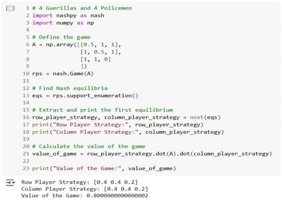
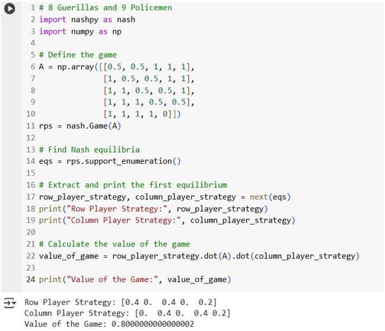
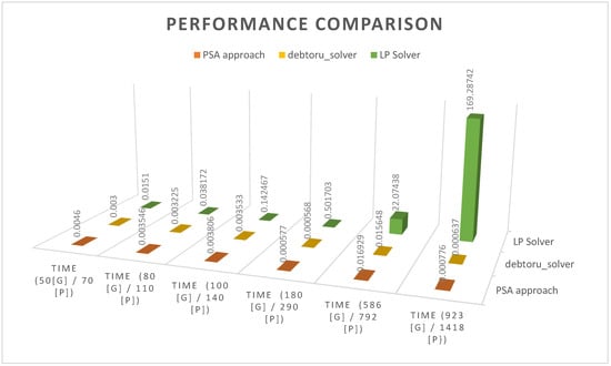
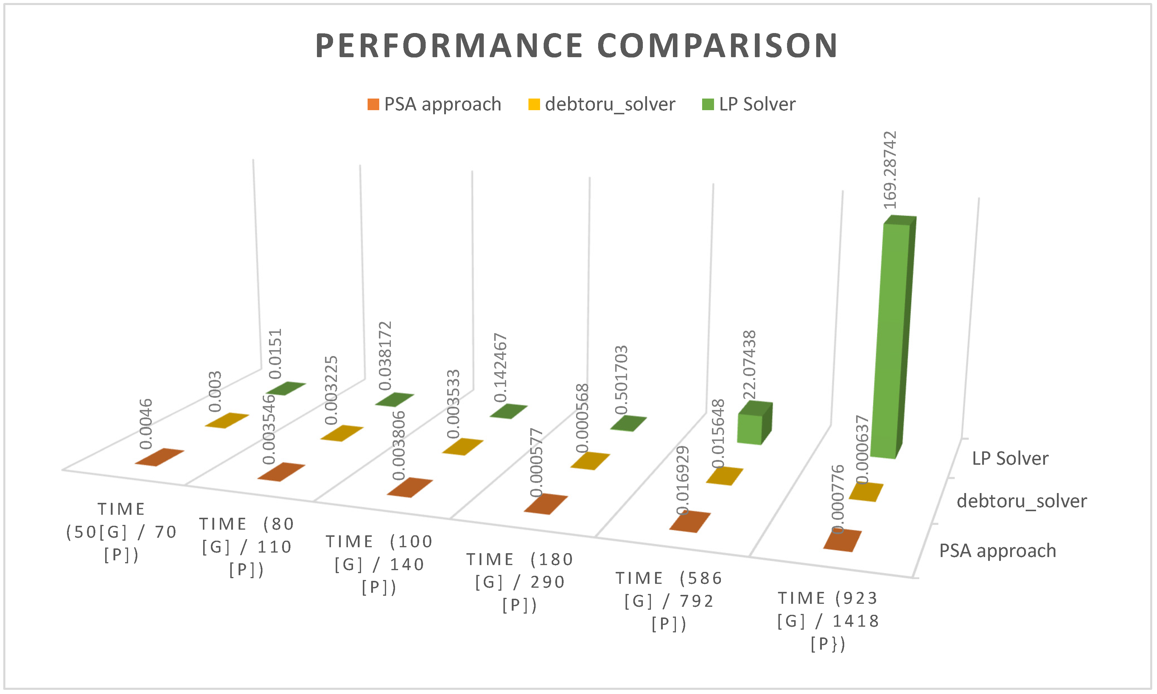

Disclaimer/Publisher’s Note: The statements, opinions and data contained in all publications are solely those of the individual author(s) and contributor(s) and not of MDPI and/or the editor(s). MDPI and/or the editor(s) disclaim responsibility for any injury to people or property resulting from any ideas, methods, instructions or products referred to in the content. |
© 2026 by the authors. Licensee MDPI, Basel, Switzerland. This article is an open access article distributed under the terms and conditions of the Creative Commons Attribution (CC BY) license.