Optimal Design of Non-Linear Fuzzy Inference Controllers via Black-Backed Jackal Optimization: A New Robust Bio-Inspired Framework for Industrial and Autonomous Systems

Abstract

This study introduces the ’Black-Backed Jackal Optimization’ (BBJO), a nature-inspired meta-heuristic algorithm designed for complex, non-linear, and high-dimensional search spaces. The fundamental mathematical model of BBJO relies on the opportunistic hunting behavior and survivability strategies of the black-backed jackal (Lupulella mesomelas). We use non-linear energy decrease and adaptive Lévy flight to maintain the equilibrium of the search. This allows the algorithm to scan large areas first, then zoom in with a high degree of precision once it has identified a suitable location. This configuration prevents the algorithm from getting stuck on a suboptimal local solution, which is a frequent danger during searches in complex spaces. BBJO has been validated against 23 standard benchmark functions, demonstrating significantly greater accuracy than Particle Swarm Optimization (PSO) on complex and large-scale search spaces. On fixed-size domains ($F_{21}$–$F_{23}$), the BBJO algorithm achieved a 100% success rate with zero standard deviation, surpassing the Grey Wolf Optimizer (GWO) and Differential Evolution (DE), which frequently suffered from structural stagnation. Visual convergence study shows that BBJO efficiently identifies optimal search regions early in the iteration budget, saving time compared to traditional linear decay models. BBJO optimizes fuzzy inference systems (FISs) for two practical applications: autonomous car speed control and industrial furnace regulation. Experimental results indicate that BBJO significantly decreased cumulative penalties and improved steady-state error reduction compared to baseline configurations and established meta-heuristic methods. The results show that BBJO is a reliable and useful technique for engineering optimization.

1. Introduction

Industrial automation and autonomous systems operate under conditions that conventional controllers handle poorly. In a lot of cases sensor data is imprecise, system dynamics are non-linear, and also the relationship between inputs and outputs resists exact mathematical description. To resolve this, Fuzzy Inference Systems (FISs), introduced by Zadeh [1], address these conditions through representations of linguistic variables that encode expert knowledge in a computationally tractable form. Based on this, the Mamdani inference framework [2] established the standard mapping from linguistic rules to numerical control outputs; this framework remains the basis for fuzzy controller design in engineering applications.

The performance of a fuzzy controller depends critically on the shape and position of its membership functions. For instance, centers, widths, and overlap regions must be precisely determined, while the associated rule base must remain internally consistent. However, as system complexity increases, the number of parameters needing tuning grows rapidly [3]. That is why manual tuning through trial and error becomes both time-consuming and fails to produce optimal results [4].

These factors have led to the adoption of meta-heuristic optimization as the standard approach to automated membership function design [5]. In this setup, population-based algorithms search the fuzzy parameter space without requiring gradient information, a feature that makes them applicable to objective functions such as the Integral of Time-weighted Absolute Error (ITAE) that are non-differentiable with respect to membership function parameters [6,7]. In the end, the combination of fuzzy logic with population-based search constitutes the current paradigm in adaptive control design [4].

1.1. Motivation and Research Gap

Safety-critical and energy-intensive systems necessitate extremely precise and stable control loop tuning. Tuning deviations in applications such as autonomous vehicle speed control [8] and industrial furnace regulation [9] can cause mechanical failures, compromise passenger safety, or result in significant energy losses [6].

Gradient-based methods like backpropagation and steepest descent are poorly suited to this class of problem. The parameter space of a fuzzy controller is characterized by flat regions where the gradient drops, discontinuous surfaces, and numerous local optima that trap descent-based optimizers [4]. Furthermore, the mapping between membership function parameters and performance indices such as ITAE or IAE is generally non-differentiable, which prevents the direct application of analytical optimization [7].

The principal limitation of existing meta-heuristic algorithms is the rigidity of their phase-transition mechanisms. Most established methods govern the exploration–exploitation balance through a linear parameter decay, but this schedule does not reflect the non-linear behavioral shifts observed in biological foraging, leading to premature convergence: the algorithm commits to local refinement before the global search space has been adequately sampled [6].

A second limitation is the gap between benchmark performance and performance on engineering optimization problems. Fuzzy surfaces are characterized by extended plateau regions where the objective function is insensitive to parameter perturbations, and by narrow high-gradient ridges where the global optimum is located. These features are not represented in classical unimodal or separable benchmark functions [6].

There is currently no framework that integrates a heavy-tailed foraging operator, biologically grounded pair-based leadership, and non-linear energy decay into a single structure calibrated for FIS tuning. BBJO is introduced to address this set of limitations. Population-based and gradient-free optimizers navigate the search space through stochastic sampling rather than derivative information and are capable of operating on objective functions that are non-convex, discontinuous, or computationally expensive to evaluate.

1.2. The Philosophy of Opportunistic Search

The design of BBJO is grounded in the foraging ecology of Lupulella mesomelas, the black-backed jackal. Empirical studies on animal movement confirm that efficient foragers do not sample the environment uniformly. Optimal foraging results in heavy-tailed displacement distributions in unpredictable or food-scarce situations, with many short relocations interspersed with infrequent long-range jumps. This pattern is compatible with Lévy statistics [10]. This movement structure maximizes the probability of locating resources in unknown terrain and is the biological basis for the Lévy flight operator in BBJO.

The black-backed jackal is characterized by its behavioral adaptability, altering its hunting tactics depending on its own energy levels and the behavior of its prey [11]. This adaptive behavior, switching from high-speed pursuit to targeted harassment as stamina drops, offers the biological inspiration for the exploration/exploitation trade-off in the BBJO framework. Instead of a linear schedule, BBJO models the transition with a parabolic energy decay function, which allows for a gradual and highly controlled change in search pressure over the iteration budget, avoiding abrupt transitions and enabling more stable refinement as the limit is approached.

1.3. Research Contributions

The primary contributions of this paper are as follows:

• Adaptive Energy Mechanism with Non-Linear Decay. To control the transition between exploration and exploitation, we introduce a parabolic energy parameter $E\left(t\right)=2(1-{(t/T)}^2)$. This results in a slower decay than a linear schedule, keeping global mobility active for longer and concentrating the exploitation budget in the final iterations where accuracy is more crucial.
• Pair-Based Cooperative Update with Lévy Displacement. In the phase of exploration ($\left|E\right|\ge 1$), each agent moves to the arithmetic mean of three directional candidates derived from the dominant male $X_m$, the dominant female $X_f$, and the global best $X^{*}$ (Equations (3)–(6)). The three impact vectors are rarely coincident in practice because the stochastic coefficients $A_k$ and $C_k$ change the step magnitude individually for each leader. A Lévy displacement (Equation (9), $\beta =1.5$) is then added, whose heavy-tailed distribution produces occasional long-range jumps that help agents escape deceptive local basins.
• Quadratic Prey Refinement. We develop a non-linear exploitation operator in which the step size toward the global best scales quadratically with distance. This results in higher attraction when the agent is far from $X^{*}$ and finer correction in its immediate neighborhood, which reduces oscillatory behavior during the final convergence phase.
• Validation on 23 Benchmark Functions and Two Engineering Applications. BBJO is compared with GWO, PSO, and DE on 23 mathematical benchmark functions and against 13 meta-heuristic algorithms on two non-linear FIS tuning problems: autonomous vehicle speed regulation and industrial furnace temperature regulation.

1.4. Paper Organization

Section 2 reviews the state of the art. Section 3 presents the biological foundations. Section 4 develops the mathematical model. Section 5 analyses convergence and complexity. Section 6 defines the FIS optimization problems. Section 7 presents comparative results. Section 8 concludes the paper.

2. State of the Art and Taxonomic Evolution

Meta-heuristic optimization is generally based on three paradigms: evolutionary computing (EAs), trajectory or physics-based formulations and swarm intelligence (SI) techniques. Each of the frameworks attempts to address one fundamental problem, albeit with different underlying metaphors: how to efficiently balance exploration of the space and refinement of local solutions on complex, non-linear error surfaces.

The No Free Lunch theorem [12] is the baseline constraint for this entire domain. This shows that there is no optimization procedure that can beat all other methods in all possible problem instances. Any gain in performance on one class of problems is quantitatively balanced by poor performance on others. There is no default to choose or build an optimization tool. This is a basic design choice that requires a deep understanding of the mathematical properties of the system to be targeted.

Evolutionary algorithms (EAs) are optimization algorithms that iteratively improve a population of potential solutions by utilizing natural selection mechanisms like genetic crossover and mutation. Holland’s Genetic Algorithm (GA) [13] serves as the foundation for this course. Goldberg [14] later expanded it to practical engineering scenarios. A theory influenced by evolution is called Differential Evolution (DE) [15]. By working directly on real vectors and generating trial states from vector differences of random agents, DE automatically adjusts to the local topology of the search space. It can be used for tasks involving continual optimization because of this feature. This includes fuzzy membership function calibration.

Later evolutionary designs incorporated broader ecological or behavioral concepts. Biogeography-Based Optimization (BBO) [16] treats solution vectors as habitats and uses migratory models to propagate superior features prior to being eliminated by selection pressures. Other methods regulate exploration by giving specific roles to the population. The Artificial Bee Colony (ABC) algorithm [17] separates agents into employed bees, onlookers and scouts in order to carry out specific search behaviors. Cultural Algorithms (CA) [18] retain and utilize global knowledge between generations in an auxiliary belief space. The Covariance Matrix Adaptation Evolution Strategy (CMA-ES) [19] provides a rigorous alternative for very ill-conditioned landscapes. It keeps a full covariance matrix of the search distribution, which is continuously adjusted to track the exact mathematical curvature of the cost function.

Physics-based approaches use explicit physical laws (not biological metaphors) to determine the movements of agents. The Gravitational Search Algorithm (GSA) [20] views potential solutions as physical masses interacting with each other through Newtonian attraction. High-fitness agents act as heavy masses, attracting lighter agents to promising regions. In a similar fashion, the Archimedes Optimization Algorithm (AOA) [21] employs Archimedes’ principle of fluid buoyancy and immersion depth for agent displacement control, balancing convergence pressure with repulsion loops.

Other physics-inspired approaches simulate thermodynamic or cosmological equilibrium situations. The Sine Cosine Algorithm (SCA) [22] applies simple trigonometric equations to generate oscillatory motions, which compel the agents to alternate between wide exploration and local exploitation. The Multi-Verse Optimizer (MVO) [23] is based on the cosmology concepts and utilizes white holes, black holes and wormholes to control the solution transfers. On the other hand, the Equilibrium Optimizer (EO) [24] is based on mass balance equations in a control volume to formulate its search rules. The mass balance approach is structurally similar to other specialized physics solvers such as Henry Gas Solubility Optimization (HGSO) [25], Thermal Exchange Optimization (TEO) [26], and the Crystal Structure Algorithm (CryStAl) [27].

Swarm intelligence (SI) is concerned with the emergence of a global behavior in groups of animals based on simple local interactions. Particle Swarm Optimization (PSO) [28] is still the classic paradigm in this kind. PSO is inspired by bird flocking and updates particle velocities from a combination of personal historical best positions and the global optimum of the swarm. PSO is easy to implement and computationally inexpensive. However, PSO tends to lose population diversity fast and tend to get stuck in local minima for complex multimodal landscapes.

The problem of premature convergence is addressed by numerous modern SI frameworks. In order to stabilize the transition between exploration and exploitation, the Grey Wolf Optimizer (GWO) [29] uses a strict three-tier social hierarchy (alpha, beta, and delta leaders) to direct an encircling approach. The Whale Optimization Algorithm (WOA) [30] uses a logarithmic spiral model for local updates to simulate the bubble-net feeding behavior of whales. A alternative topological structure is used by the Salp Swarm Algorithm (SSA) [31], where agents are connected in a linear chain and each salp follows the salp in front of it to maintain a wide population spread.

In order to find alternative behavioral splits, the Sparrow Search Algorithm (SpSA) [32] divides the agents into producers and scroungers and adds a predator avoidance trigger. The Firefly Algorithm (FA) [33,34] is based on the attraction of light intensity, where brightness is determined by a solution’s quality and decreases with distance. So as to smoothly transition between four distinct cooperative hunting modes, Harris Hawks Optimization (HHO) [35] uses an energy parameter. In order to preserve variety of search, the Dung Beetle Optimizer (DBO) [36] uses rolling, foraging, and stealing behaviors among several subpopulations.

Mathematical operators and highly specialized ecological niches are recent themes in SI. While the Crested Porcupine Optimizer (CPO) [37] uses a four-phase defensive model to maintain population diversity, the Artificial Hummingbird Algorithm (AHA) [38] looks for limited local solutions. While the Mantis Search Algorithm (MSA) [39] alternates between static ambush and active strike, the Nutcracker Optimization Algorithm (NOA) [40] is based on spatial memory. Frameworks such as the Zebra Optimization Algorithm (ZOA) [41] and associated meta-heuristics [42,43] use Lévy flights [10] with power-law step variations for effective coverage of large search domains to enhance global exploration. The Golden Jackal Optimization (GJO) [44], the African Vulture Optimization Algorithm (AVOA) [45], Teaching-Learning-Based Optimization (TLBO) [46], Jaya [47], Moth-Flame Optimization (MFO) [48], the Ant Lion Optimizer (ALO) [49], and the Bat Algorithm (BAT) [50] are also covered by this vast area.

In recent years, the taxonomy of bio-inspired meta-heuristics has expanded significantly with the introduction of highly specialized swarm-based frameworks. Notable examples include the Zebra Optimization Algorithm (ZOA) [41], which models the foraging and anti-predator behaviors of zebras, and the Mantis Search Algorithm (MSA) [39], which mathematically replicates the unique hunting and clutching mechanics of praying mantises. While these contemporary algorithms introduce sophisticated multi-phase kinematic rules to balance exploration and exploitation, they fundamentally belong to the class of leader-follower or pattern-based localized search paradigms. Consequently, they often encounter structural vulnerabilities—such as asymptotic stagnation—when navigating high-dimensional, highly non-convex landscapes where gradient trajectories disappear. The proposed BBJO breaks from these rigid step-wise frameworks by introducing a heavy-tailed Lévy flight component coupled with an adaptive metabolic energy decay model, offering a fundamentally different mathematical approach to overcoming localized traps.

Yet, none of the existing methods capture this specific dual-leader hierarchy, the non-linear metabolic stamina depletion and opportunistic scavenging traits of Lupulella mesomelas within this wide range of biological and physical metaphors. Simple linear or uniform random decay schedules are the foundation of current energy-driven techniques like GJO and AVOA. These functions do not correspond to a predator’s actual physiological weariness curve after a protracted hunt. The optimization landscape for adjusting fuzzy inference systems (FISs) is made up of small high-gradient valleys between flat plateaus. The inflexible, linear transitions between exploration and exploitation cause these algorithms to either stall early or fail to refine the membership function limits. Black-Backed Jackal Optimization (BBJO) was developed in response to this problem. In order to overcome these structural constraints and improve convergence accuracy, BBJO incorporates a cooperative flanking operator and a parabolic energy decay model.

3. Biological Foundations and Inspiration: The Black-Backed Jackal

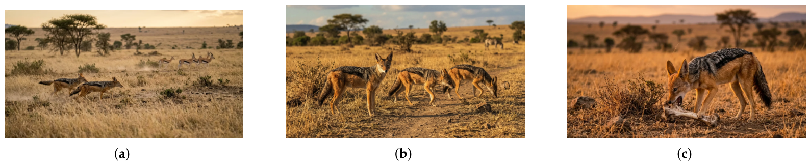
Compared to single-strategy predators, Lupulella mesomelas maximizes survival by opportunistically adapting its hunting role dependent on energy levels and environmental factors [11,51]. It alternates between territorial sentinel responsibilities, scavenging, and active hunting with ease. These behavioral shifts are mathematically mapped into the dynamic energy parameter $\left|E\right|$ via the BBJO framework. The swarm can either engage in direct carcass scavenging, cooperative pair hunting, or loose-group foraging with a sentinel, depending on this threshold (Figure 1).

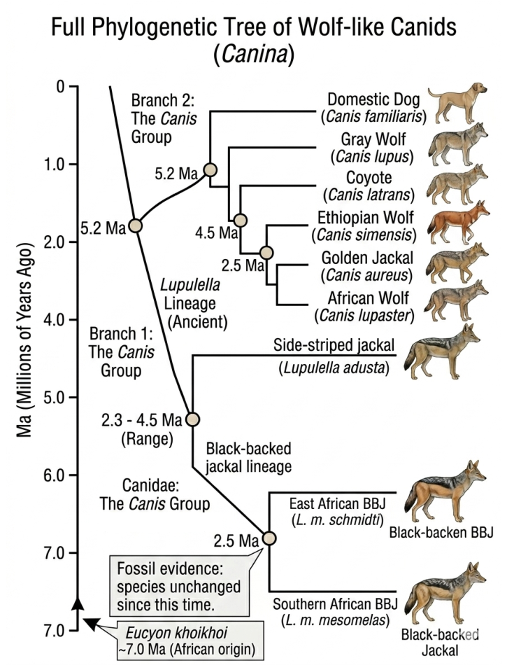
As the phylogenetic tree in Figure 2 reveals, L. mesomelas branched off from other wolf-like canids approximately 5.2 million years ago [53], predating the entire modern Canis radiation. Fossil evidence further indicates that the species has remained morphologically stable for approximately 2.5 million years [54]—a testament to the effectiveness of its generalist strategy [52].

3.1. Pair-Based Hierarchical Leadership

Jackals usually hunt in pairs. However, they can gather in larger groups to chase big prey [55]. Their movement decisions come from a clear negotiation between dominant and sub-dominant members [56]. The BBJO algorithm selects two elite candidates at each iteration. These are the dominant male $X_m$ and the dominant female $X_f$, which represent the best and second-best solutions. A third component, the global best $X^{*}$, is also used. It pulls the group toward the most promising area. This independent pull from $X^{*}$ is useful. Even if both leaders get stuck in the same local optimum, $X^{*}$ helps maintain directional diversity.

3.2. The Fatigue Principle and Non-Linear Search Pressure

The hunting intensity of L. mesomelas depends on its metabolic stamina and the energy needed for the chase [57]. At first, the predator uses high-velocity exploration. When its stamina drops, it switches to a low-energy approach [58]. The BBJO algorithm models this using the Adaptive Energy Mechanism $E\left(t\right)$. This mechanism uses a parabolic decay function $(1-{(t/T)}^2)$. It keeps global mobility high while $\left|E\right|\ge 1$. Then, it switches to the Quadratic Prey Refinement operator when $\left|E\right|<1$. This switch reduces the exploitation budget in the final iterations to focus strictly on precision.

3.3. The Generalist Spectrum: Scavenging and Foraging

• Non-Gaussian Foraging (Exploration): When food is scarce, L. mesomelas travels using heavy-tailed patterns. This means they take many regular short steps combined with occasional long-distance jumps [59]. BBJO models this behavior through Lévy flights (Equation (9)) during the exploration phase when $\left|E\right|\ge 1$. This mechanism helps the agents escape from local traps in complex multimodal landscapes.
• Opportunistic Scavenging (Exploitation): Jackals can travel long distances to use found resources. They do this by watching social cues [60]. When they find a high-value resource, their random movement stops and they move directly toward it. The Scavenging Mechanism (Equation (13)) activates with a probability $P_{scav}$. This mechanism pulls the agents directly toward the current global best $X^{*}$.

3.4. Adaptive Vigilance and Risk Evasion

When feeding near larger competitors such as lions or hyenas, L. mesomelas makes sudden erratic directional shifts. The Random Jump Mechanism (Equation (14)) mimics this behavior, applied independently with probability $P_r$ after all positional updates. The perturbation magnitude is calibrated to be small enough not to displace well-converged agents, yet frequent enough to prevent premature settling.

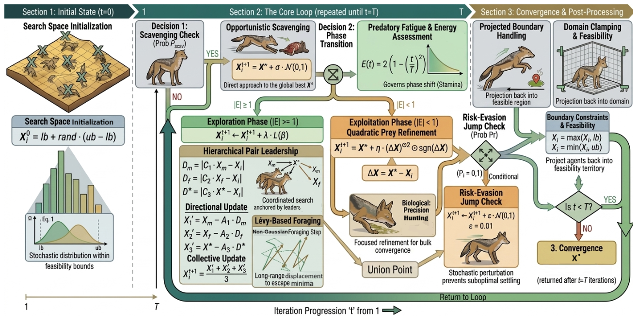
Figure 3 consolidates the mappings between the three behavioral modes and BBJO’s mathematical operators, showing how $\left|E\right|$ governs the transition across the full iteration cycle.

4. Mathematical Model and Framework of BBJO

4.1. Search Space Initialization and Agent Distribution

The optimization process begins with the stochastic distribution of N agents across a d-dimensional search domain $\mathsf{\Omega }\subset {\mathbb{R}}^d$:

$$X_i^0=lb+rand·(ub-lb),i=1,\dots ,N,$$

(1)

where $lb$ and $ub$ are the lower and upper boundaries, and $rand\sim \mathcal{U}(0,1)$.

4.2. Hierarchical Pair Leadership and Group Hunting

BBJO identifies two elite candidates at each iteration t [55]: the dominant male $X_m$ and the dominant female $X_f$ (best and second-best agents). The global best $X^{*}$ is updated whenever a superior fitness value is encountered:

$$X^{*}\leftarrow X_i\mathrm{if}f\left(X_i\right)<f\left(X^{*}\right).$$

(2)

The spatial influence of each leader on agent $X_i$ is quantified through distance vectors and associated directional updates:

$$\begin{array}{cc}\hfill D_m& =\left|C_1·X_m-X_i\right|,X_1^{\prime }=X_m-A_1·D_m\hfill \end{array}$$

(3)

$$\begin{array}{cc}\hfill D_f& =\left|C_2·X_f-X_i\right|,X_2^{\prime }=X_f-A_2·D_f.\hfill \end{array}$$

(4)

A third directional component is derived from the global best $X^{*}$:

$$D^{*}=\left|C_3·X^{*}-X_i\right|,X_3^{\prime }=X^{*}-A_3·D^{*}.$$

(5)

The collective position update is the arithmetic mean of these three coordinated trajectories:

$$X_i^{t+1}={\displaystyle \frac{X_1^{\prime }+X_2^{\prime }+X_3^{\prime }}{3}}.$$

(6)

The stochastic coefficients $A_k$ and $C_k$ introduce variability to simulate unpredictable pursuit paths:

$$A_k={\alpha }_0(2r_k-1),C_k=2r_k,r_k\sim \mathcal{U}(0,1),$$

(7)

where ${\alpha }_0=2$ is held constant throughout the run, allowing agents to overshoot their leaders and sustain global exploration in later iterations.

4.3. Predatory Fatigue and Phase Transition

The Adaptive Energy Mechanism $E\left(t\right)$ [57] governs the transition from global exploration to local refinement via a parabolic decay:

$$E\left(t\right)=2\left(1-{\left({\displaystyle \frac{t}{T}}\right)}^2\right),$$

(8)

where T is the maximum number of iterations. The magnitude $\left|E\right|$ selects the active behavioral phase of every agent at each iteration.

4.3.1. Exploration Phase: Lévy-Based Foraging

When $\left|E\right|\ge 1$, agents operate through the cooperative leadership update of Equation (6), augmented by a Lévy flight displacement:

$$X_i^{t+1}\leftarrow X_i^{t+1}+\lambda ·L\left(\beta \right),$$

(9)

where $\lambda$ scales the step magnitude and $L\left(\beta \right)$ is a Lévy-stable random vector with index $\beta =1.5$, generated via Mantegna’s algorithm [61]:

$$L_j={\displaystyle \frac{u_j}{|v_j{|}^{1/\beta }}},u_j\sim \mathcal{N}(0,{\sigma }^2),v_j\sim \mathcal{N}(0,1),$$

(10)

$$\sigma ={\left({\displaystyle \frac{\Gamma (1+\beta )sin(\pi \beta /2)}{\Gamma \left(\frac{1+\beta }{2}\right)\beta 2^{(\beta -1)/2}}}\right)}^{1/\beta }.$$

(11)

The heavy tail of $L\left(\beta \right)$ generates rare long-range jumps, allowing agents to exit deceptive basins.

4.3.2. Exploitation Phase: Quadratic Prey Refinement

When $\left|E\right|<1$, the agent transitions to precision refinement [58]:

$$\begin{array}{cc}\hfill \Delta X& =X^{*}-X_i\hfill \\ \hfill X_i^{t+1}& =X^{*}+\eta ·{(\Delta X)}^{\odot 2}\odot sgn(\Delta X),\hfill \end{array}$$

(12)

where $\eta$ is the exploitation coefficient and ⊙ denotes element-wise multiplication. The squared displacement applies stronger attraction when the agent is distant from $X^{*}$ and progressively gentler correction nearby, accelerating convergence without collapsing the population to a single point.

4.4. Generalist Strategies: Scavenging and Vigilance

Opportunistic Scavenging. With probability $P_{scav}$, an agent bypasses the energy-conditioned branching and moves directly toward the global best [60]:

$$X_i^{t+1}=X^{*}+\sigma ·\mathcal{N}(0,1),$$

(13)

where $\sigma =0.05$. This mechanism is evaluated first at each iteration, prior to the energy-conditioned update.

Risk-Evasion Jump. Applied independently with probability $P_r$ after all positional updates:

$$X_i^{t+1}\leftarrow X_i^{t+1}+ϵ·\mathcal{N}(0,1),$$

(14)

where $ϵ=0.01$ and $P_r=0.1$. After every update, agents are projected back into the feasible domain:

$$X_i=max(X_i,lb),X_i=min(X_i,ub).$$

(15)

4.5. BBJO Metaheuristic Procedure

The complete operational flow of BBJO is summarized in Algorithm 1 and

Table 1. BBJO parameter summary.

Parameter	Symbol	Value	Biological Meaning
Exploration scale	${\alpha }_0$	2.0	Hunt aggression
Exploitation coeff.	$\eta$	0.5	Late-stage precision
Scavenging prob.	$P_{scav}$	0.25	Carcass detection rate
Risk-evasion prob.	$P_r$	0.1	Competitor-induced evasion
Lévy scale	$\lambda$	0.01	Long-range step amplitude
Lévy index	$\beta$	1.5	Step-length tail weight
Scavenging noise	$\sigma$	0.05	Neighborhood radius around $X^{*}$
Evasion noise	$ϵ$	0.01	Evasion displacement

.

Algorithm 1: Black-Backed Jackal Optimization (BBJO)

5. Convergence and Computational Complexity Analysis

5.1. Probabilistic Convergence Analysis

While proving global optimality is very difficult for stochastic meta-heuristics, BBJO ensures convergence through a high-probability framework. This framework relies on four main structural properties.

Exploration and Exploitation Balance. The adaptive energy parameter $E\left(t\right)=2(1-{(t/T)}^2)$ keeps $\left|E\right|\ge 1$ during the early iterations. This forces the agents to explore wide areas. Near the maximum iteration T, the parabolic decay drops faster than a simple linear model. This rapid drop speeds up the transition to the exploitation phase. It also concentrates the computing power on local refinement during the final steps.

Pair Leadership and Directional Diversity. The collective update formula $X_i^{t+1}=(X_1^{\prime }+X_2^{\prime }+X_3^{\prime })/3$ splits the influence among three independent vectors. This setup reduces directional bias compared to models that use only a single leader. As a result, it helps preserve population diversity throughout the entire execution.

Lévy Flights and Global Ergodicity. During the exploration phase, Lévy flights create heavy-tailed and long-range jumps: $X_i^{t+1}\leftarrow X_i^{t+1}+\lambda ·L\left(\beta \right)$. This movement ensures that the search process is ergodic. This means that any part of the search space $\mathsf{\Omega }$ can still be reached at any iteration [62]. This property is the main tool used to avoid getting stuck in deceptive local optima.

Quadratic Refinement and Stable Convergence. In the exploitation phase, the step size drops quadratically as $\Delta X\to 0$. This behavior removes the oscillations that often happen with linear update rules. In linear rules, the step size stays proportional to the distance, even close to $X^{*}$. Here, the quadratic approach ensures a much more stable convergence.

5.2. Computational Complexity Analysis

The computational complexity is evaluated using the population size N, the dimensionality D, the maximum number of iterations T, and the objective function evaluation cost $C_{obj}$.

Proposition 1. 

The total time complexity of BBJO is given by ${\mathcal{T}}_{BBJO}=\mathcal{O}(T·[f(N,D)+N·C_{obj}])$.

Proof. 

The initialization step requires $\mathcal{O}(N·D)$ operations. During each iteration, evaluating the fitness of the population costs $N·C_{obj}$. This evaluation step dominates the runtime in FIS tuning applications because $C_{obj}$ requires a complete inference simulation. Finding the leaders $X_m$ and $X_f$ involves a basic sorting operation, which costs $\mathcal{O}(NlogN)$. The rest of the position updates are performed element-wise across the D coordinates for each agent, costing $\mathcal{O}(N·D)$. By defining $f(N,D)=\mathcal{O}(NlogN+ND)$ and neglecting the initialization cost for large values of T, we obtain the final expression. □

Proposition 2. 

The space complexity of BBJO is bounded by $\mathcal{S}=\mathcal{O}(N·D)$, which corresponds to a memory multiplier $k=1$.

Proof. 

The main data structure used in the algorithm is the population position matrix $\mathbf{X}\in {\mathbb{R}}^{N\times D}$, requiring ${\mathcal{S}}_{pop}=ND$ storage. Additionally, the algorithm stores the vectors for the two leaders and the global best solution, which takes ${\mathcal{S}}_{elite}=3D$. The scalar auxiliary buffers require minimal memory, represented as ${\mathcal{S}}_{aux}=\mathcal{O}\left(D\right)$. Because BBJO performs all position updates in-place, it does not need to store separate trial or mutant matrices. Therefore, the total memory allocation remains ${\mathcal{S}}_{total}\approx N·D$, meaning $k=1$. This structural choice is more efficient than other algorithms like PSO, which requires $k=3$ due to separate velocity and personal-best matrices, or DE and BAT, which require $k=2$. □

Table 2. Temporal and spatial complexity of the 14 meta-heuristic optimizers.

Algorithm	Time: $\mathit{f}(\mathit{N},\mathit{D})$	Space: k	Internal Logic
PSO	$\mathcal{O}(N·D)$	3	Velocity and personal best
GWO	$\mathcal{O}(N·D)$	1	Alpha/Beta hierarchy
DE	$\mathcal{O}(N·D)$	2	Mutant/trial vectors
BBJO	$\mathcal{O}(\mathbf{N}·\mathbf{D}+\mathbf{N}log\mathbf{N})$	1	Lévy + quadratic refinement
FA	$\mathcal{O}(N^2·D)$	1	All-to-all comparison
TLBO	$\mathcal{O}(N·D)$	1	Teacher/learner phases (two-pass)
MFO	$\mathcal{O}(NlogN+N·D)$	2	Flame sorting
WOA	$\mathcal{O}(N·D)$	1	Spiral bubble-net
SCA	$\mathcal{O}(N·D)$	1	Sine-cosine periodicity
HHO	$\mathcal{O}(N·D)$	1	Multi-stage besiege
ALO	$\mathcal{O}(NlogN+N·D)$	2	Random walk and sorting
Jaya	$\mathcal{O}(N·D)$	1	Best/worst attraction
BAT	$\mathcal{O}(N·D)$	2	Frequency/loudness
SSA	$\mathcal{O}(N·D)$	1	Leader-follower chain

compares the complexity of all 14 meta-heuristics considered in this study. FA incurs a quadratic bottleneck at $\mathcal{O}(N^2·D)$ from all-to-all pairwise comparisons. BBJO operates in the same linear-time tier as GWO, WOA, and HHO, while its $k=1$ memory footprint makes it three times more efficient than PSO—a relevant advantage in embedded FIS applications.

6. Optimal Design of Fuzzy Controllers via BBJO

6.1. Fuzzy Speed Regulator for Autonomous Vehicles

6.1.1. Problem Description

The Speed Regulator manages the longitudinal movement of an autonomous vehicle. Its primary task is to maintain a safe headway behind a leading vehicle while adjusting speed smoothly [8,63]. The optimization setup balances two operational goals. First, Tracking Precision focuses on reducing spacing errors to improve distance tracking. Second, Comfort requires minimizing vehicle jerk, defined as the rate of change of acceleration, to prevent sudden switching between throttle and braking controls.

6.1.2. FIS System Description

A Mamdani-type FIS with two inputs and a single output handles the control inference.

Table 3. Linguistic variable definitions for the Speed Regulator FIS.

Variable	Role	Label	Meaning
Distance d (m)	Input	Close	Short following gap
		Medium	Safe headway
		Far	Large following gap
Velocity v (m/s)	Input	Slow	Low speed
		Medium	Moderate speed
		Fast	High speed
Acceleration a (m/s2)	Output	Hard brake	Strong deceleration
		Light brake	Gentle deceleration
		Stable	Maintain speed
		Light accel.	Gentle acceleration
		Hard accel.	Strong acceleration

summarizes the linguistic variables and their associated sets.

Inputs and Outputs with Linguistic Sets:

Fuzzy Rule Base:

• If d is Close and v is Fast ⇒ Hard brake.
• If d is Close and v is Medium ⇒ Light brake.
• If d is Medium and v is Fast ⇒ Light brake.
• If d is Medium and v is Medium ⇒ Stable.
• If d is Far and v is Slow ⇒ Hard accel.
• If d is Far and v is Medium ⇒ Light accel.

6.1.3. Optimization Variables, Constraints, and Objective

The decision vector ${\mathbf{X}}_1\in {\mathbb{R}}^{22}$ defines all tunable membership function vertices within the FIS. Monotonicity conditions enforce strict linguistic ordering:

$$\left\{\begin{array}{c}{d}_{\mathrm{close},1}\le d_{\mathrm{close},2}\le d_{\mathrm{close},3}\le d_{\mathrm{close},4}\hfill \\ d_{\mathrm{close},3}<d_{\mathrm{medium},2}<d_{\mathrm{far},2}\hfill \\ v_{\mathrm{slow},1}\le v_{\mathrm{slow},2}\le v_{\mathrm{slow},3}\hfill \\ v_{\mathrm{slow},2}<v_{\mathrm{medium},2}<v_{\mathrm{fast},2}\hfill \end{array}\right.$$

(16)

The longitudinal dynamics of the vehicle model the evolution of relative spacing and velocity. Here, $d\left(t\right)$ represents the inter-vehicle distance and $v_{\mathrm{lead}}$ is the constant speed of the preceding vehicle during simulation. The system updates use the following kinematic equations:

$$v_{k+1}=v_k+a_k\Delta t$$

(17)

$$d_{k+1}=d_k+\left(v_{\mathrm{lead}}-v_k\right)\Delta t\kappa$$

(18)

where $\kappa =0.05$ acts as a scaling coefficient inside the simulation environment.

The cost function minimizes the tracking distance error over time alongside passenger discomfort caused by sudden changes in acceleration profile:

$$J\left({\mathbf{X}}_1\right)={\displaystyle \sum _{k=0}^K}{t}_k|d_{\mathrm{ref}}-d_k|\Delta t+\gamma \underset{k}{max}\left|j_k\right|$$

(19)

Here, $\gamma$ is the penalty weight applied to the peak jerk, balancing tracking accuracy against ride comfort. The discrete-time vehicle jerk $j_k$ is evaluated as:

$$j_k={\displaystyle \frac{a_k-a_{k-1}}{\Delta t}}$$

(20)

6.2. Smart Oven Temperature Regulation

6.2.1. Problem Description

Thermal processing in the industry requires accurate control of the heat trajectories. The main difficulty is to reach the setpoint quickly without overshoot which can cause deterioration of the material [9]. Here BBJO addresses two major problems. First, Transient Response Balancing balances the transition from maximum to maintenance power according to the remaining time. Second, Thermal Lag Compensation changes the membership functions to consider the lag between the application of energy and the measurement of temperature.

6.2.2. FIS System Description

The oven controller is built for an asymmetric cost structure. In this setup any temperature overshoot irreversibly damages the material. The time-remaining input provides the system with a sense of urgency. This context allows the controller to differentiate between similar temperatures at different points during the operation.

Table 4. Linguistic variable definitions for the Smart Oven FIS.

Variable	Role	Label	Meaning
Temperature T (°C)	Input	Cold	Below target
		Medium	Near target
		Hot	At or above target
Time Remaining t (s)	Input	Short	Little time left
		Medium	Moderate time left
		Long	Ample time left
Heating Intensity P (%)	Output	Low	Maintenance power
		Medium	Moderate heating
		High	Maximum heating

defines the linguistic variables used in this controller.

Inputs and Outputs with Linguistic Sets:

Fuzzy Rule Base (6 rules): (1) T Cold ∧ t Short ⇒ High; (2) T Cold ∧ t Long ⇒ Medium; (3) T Medium ∧ t Short ⇒ Medium; (4) T Hot ⇒ Low; (5) t Medium ∧ T Medium ⇒ Medium; (6) T Cold ∧ t Medium ⇒ High.

6.2.3. Optimization Variables, Constraints, and Objective

The decision vector ${\mathbf{X}}_2=[t_{short,i},t_{medium,i},t_{long,i},tem{p}_i,powe{r}_i]$ with constraints:

$$\left\{\begin{array}{c}{T}_{cold,\mathrm{peak}}<T_{medium,\mathrm{peak}}<T_{hot,\mathrm{peak}}\hfill \\ 0<t_{short,\mathrm{peak}}<t_{medium,\mathrm{peak}}<t_{long,\mathrm{peak}}\hfill \\ {\mathbf{X}}_{2,\mathrm{power}}\in [0,100].\hfill \end{array}\right.$$

(21)

The objective minimizes rise time $t_r$, steady-state error $e_{ss}$, and maximum overshoot $M_p$ [9]:

$$minJ\left({\mathbf{X}}_2\right)={\omega }_1·t_r+{\omega }_2·|T_{target}-T_{final}|+{\omega }_3·M_p.$$

(22)

7. Comparative Results and Discussion

7.1. Comparison on Benchmark Problems

7.1.1. Benchmark Functions Description

Three different topological classes cover the 23 benchmark functions.

Table 5. Unimodal benchmark functions.

Function	Dim	Range	${\mathit{f}}_{min}$
$f_1\left(x\right)={\sum }_{i=1}^n{x}_i^2$	30	$[-100,100]$	0
$f_2\left(x\right)={\sum }_{i=1}^n\left|x_i\right|+{\prod }_{i=1}^n\left|x_i\right|$	30	$[-10,10]$	0
$f_3\left(x\right)={\sum }_{i=1}^n{\left({\sum }_{j=1}^i{x}_j\right)}^2$	30	$[-100,100]$	0
$f_4\left(x\right)=max\left\{\right|x_i|,1\le i\le n\}$	30	$[-100,100]$	0
$f_5\left(x\right)={\sum }_{i=1}^{n-1}\left[100{(x_{i+1}-x_i^2)}^2+{(x_i-1)}^2\right]$	30	$[-30,30]$	0
$f_6\left(x\right)={\sum }_{i=1}^n{(x_i+0.5)}^2$	30	$[-100,100]$	0
$f_7\left(x\right)={\sum }_{i=1}^{n}i{x}_i^4+\mathrm{rand}[0,1]$	30	$[-1.28,1.28]$	0

contains seven unimodal functions in the first group, which range from $f_1$ to $f_7$. These functions, which are used to evaluate raw exploitation speed, lack local optima. Six high-dimensional multimodal functions, ranging from $f_8$ to $f_{13}$ in

Table 6. Multimodal benchmark functions (high-dimensional).

Function	Dim	Range	${\mathit{f}}_{min}$
$f_8\left(x\right)={\sum }_{i=1}^n-x_{i}sin\left(\sqrt{|x_i|}\right)$	30	$[-500,500]$	$-418.9\times n$
$f_9\left(x\right)={\sum }_{i=1}^n[x_i^2-10cos\left(2\pi x_i\right)+10]$	30	$[-5.12,5.12]$	0
$f_{10}\left(x\right)=-20exp\left(-0.2\sqrt{\frac{1}{n}\sum x_i^2}\right)-exp\left(\frac{1}{n}\sum cos\left(2\pi x_i\right)\right)+20+e$	30	$[-32,32]$	0
$f_{11}\left(x\right)=\frac{1}{4000}\sum x_i^2-\prod cos\left(\frac{x_i}{\sqrt{i}}\right)+1$	30	$[-600,600]$	0
$f_{12}\left(x\right)=\frac{\pi }{n}\left[10{sin}^2\left(\pi y_1\right)+\sum {(y_i-1)}^2(1+10{sin}^2\left(\pi y_{i+1}\right))+{(y_n-1)}^2\right]+\sum u(x_i,10,100,4)$	30	$[-50,50]$	0
$f_{13}\left(x\right)=0.1\left[{sin}^2\left(3\pi x_1\right)+\sum {(x_i-1)}^2(1+{sin}^2(3\pi x_i+1))+{(x_n-1)}^2(1+{sin}^2\left(2\pi x_n\right))\right]+\sum u(x_i,5,100,4)$	30	$[-50,50]$	0

, make up the second group. These functions assess the Lévy flight operator’s capacity to avoid local traps. Ten fixed-dimension functions, from $f_{14}$ to $f_{23}$, are included in the third group in

Table 7. Fixed-dimension multimodal benchmark functions.

Function	Dim	Range	${\mathit{f}}_{min}$
$f_{14}\left(x\right)={\left(\frac{1}{500}+{\sum }_{j=1}^{25}\frac{1}{j+\sum {(x_i-a_{ij})}^6}\right)}^{-1}$	2	$[-65,65]$	1
$f_{15}\left(x\right)={\sum }_{i=1}^{11}{\left[a_i-\frac{x_1(b_i^2+b_i{x}_2)}{b_i^2+b_i{x}_3+x_4}\right]}^2$	4	$[-5,5]$	0.00030
$f_{16}\left(x\right)=4x_1^2-2.1x_1^4+\frac{x_1^6}{3}+x_1{x}_2-4x_2^2+4x_2^4$	2	$[-5,5]$	$-1.0316$
$f_{17}\left(x\right)={\left(x_2-\frac{5.1}{4{\pi }^2}{x}_1^2+\frac{5}{\pi }{x}_1-6\right)}^2+10\left(1-\frac{1}{8\pi }\right)cos{x}_1+10$	2	$[-5,5]$	0.398
$f_{18}\left(x\right)=[1+{(x_1+x_2+1)}^2(19-14x_1+3x_1^2-14x_2+6x_1{x}_2+3x_2^2)]$ $\times [30+{(2x_1-3x_2)}^2(18-32x_1+12x_1^2+48x_2-36x_1{x}_2+27x_2^2)]$	2	$[-2,2]$	3
$f_{19}\left(x\right)=-{\sum }_{i=1}^4{c}_{i}exp\left(-\sum a_{ij}{(x_j-p_{ij})}^2\right)$	3	$[1,3]$	$-3.86$
$f_{20}\left(x\right)=-{\sum }_{i=1}^4{c}_{i}exp\left(-{\sum }_{j=1}^6{a}_{ij}{(x_j-p_{ij})}^2\right)$	6	$[0,1]$	$-3.3224$
$f_{21}\left(x\right)=-{\sum }_{i=1}^5{\left[(X-a_i){(X-a_i)}^T+c_i\right]}^{-1}$	4	$[0,10]$	$-10.1532$
$f_{22}\left(x\right)=-{\sum }_{i=1}^7{\left[(X-a_i){(X-a_i)}^T+c_i\right]}^{-1}$	4	$[0,10]$	$-10.4029$
$f_{23}\left(x\right)=-{\sum }_{i=1}^{10}{\left[(X-a_i){(X-a_i)}^T+c_i\right]}^{-1}$	4	$[0,10]$	$-10.5363$

. The topologies of these functions are extremely complicated but low-dimensional. The Shekel family in particular tests the algorithm for premature convergence, from $f_{21}$ to $f_{23}$, inside this group.

Every result is averaged across 30 separate runs to guarantee statistical reliability. Every run begins with a new initial population that has been randomly selected. The three baselines are chosen to represent the principal paradigms in the field: PSO [28] is the canonical swarm reference and the most widely used benchmark in the meta-heuristic literature; GWO [29] belongs to the same canid-inspired family as BBJO and therefore constitutes the most relevant biological peer; and DE [15] is retained as a strong non-swarm representative, since its differential mutation operator is particularly effective on complex, multimodal landscapes of the type considered here. For the more complex FIS tuning issues discussed in Section 7.2, the full comparison which includes all 14 algorithms is saved.

7.1.2. Statistical Comparison

To evaluate the optimization efficiency of BBJO, its performance is statistically benchmarked against three iconic foundational meta-heuristics: Grey Wolf Optimizer (GWO), Particle Swarm Optimization (PSO), and Differential Evolution (DE). This baseline selection is deliberately structured to represent distinct algorithmic mathematical paradigms, rather than merely multiplying similar behavioral models:

• PSO serves as the baseline representative for classical inertia-, velocity-, and social-attraction-driven swarm intelligence.
• DE represents the paradigm of vector-mutation and crossover-driven evolutionary algorithms.
• GWO represents strict hierarchical, encircling-based hunting mechanism, serving as a structural proxy for modern animal-behavior algorithms like the Zebra Optimization Algorithm (ZOA) or Mantis Search Algorithm (MSA), which share highly related mathematical trajectory-tracking mechanics.

By benchmarking against these three fundamentally distinct algorithmic classes, we isolate and verify the unique mathematical advantages of BBJO’s non-linear energy decay and heavy-tailed Lévy flight operator against established, mathematically well-understood search mechanics. Best, Mean, and Standard Deviation (Std) values over 30 independent runs are reported in

Table 8. Performance comparison on 23 benchmark functions (30 runs).

	GWO			PSO			DE			BBJO
Func.	Best	Mean	Std	Best	Mean	Std	Best	Mean	Std	Best	Mean	Std
F1	$2.45\times {10}^{-29}$	$7.06\times {10}^{-28}$	$7.81\times {10}^{-28}$	$4.68\times {10}^{-7}$	$3.33\times {10}^2$	$1.83\times {10}^3$	$3.28\times {10}^{-4}$	$1.12\times {10}^1$	$3.21\times {10}^1$	$6.53\times {10}^{-5}$	$1.40\times {10}^{-4}$	$3.69\times {10}^{-5}$
F2	$2.32\times {10}^{-17}$	$1.45\times {10}^{-16}$	$1.57\times {10}^{-16}$	$2.61\times {10}^{-2}$	$1.40\times {10}^1$	$1.17\times {10}^1$	$2.22\times {10}^{-4}$	$9.73\times {10}^{-2}$	$2.64\times {10}^{-1}$	$3.64\times {10}^{-2}$	$5.36\times {10}^{-2}$	$1.45\times {10}^{-2}$
F3	$2.36\times {10}^{-8}$	$1.19\times {10}^{-5}$	$2.57\times {10}^{-5}$	$3.51\times {10}^2$	$6.37\times {10}^3$	$5.58\times {10}^3$	$1.71\times {10}^2$	$6.15\times {10}^2$	$3.33\times {10}^2$	$2.18\times {10}^{-3}$	$8.89\times {10}^{-3}$	$5.15\times {10}^{-3}$
F4	$8.19\times {10}^{-8}$	$1.06\times {10}^{-6}$	$1.20\times {10}^{-6}$	$4.48\times {10}^0$	$1.04\times {10}^1$	$4.02\times {10}^0$	$1.19\times {10}^1$	$2.39\times {10}^1$	$6.54\times {10}^0$	$6.55\times {10}^{-3}$	$1.13\times {10}^{-2}$	$2.73\times {10}^{-3}$
F5	$2.61\times {10}^1$	$2.72\times {10}^1$	$6.76\times {10}^{-1}$	$1.82\times {10}^1$	$1.81\times {10}^4$	$3.66\times {10}^4$	$1.05\times {10}^2$	$2.64\times {10}^3$	$5.49\times {10}^3$	$2.69\times {10}^1$	$2.80\times {10}^1$	$4.42\times {10}^{-1}$
F6	$2.51\times {10}^{-1}$	$7.44\times {10}^{-1}$	$3.45\times {10}^{-1}$	$4.55\times {10}^{-7}$	$3.37\times {10}^2$	$1.84\times {10}^3$	$4.47\times {10}^{-4}$	$1.40\times {10}^1$	$2.25\times {10}^1$	$7.91\times {10}^{-5}$	$1.34\times {10}^{-4}$	$3.30\times {10}^{-5}$
F7	$4.94\times {10}^{-4}$	$1.97\times {10}^{-3}$	$1.14\times {10}^{-3}$	$1.78\times {10}^{-2}$	$1.77\times {10}^0$	$3.70\times {10}^0$	$3.24\times {10}^{-2}$	$1.02\times {10}^{-1}$	$7.48\times {10}^{-2}$	$6.45\times {10}^{-4}$	$5.40\times {10}^{-3}$	$2.65\times {10}^{-3}$
F8	$-7.53\times {10}^3$	$-6.20\times {10}^3$	$8.65\times {10}^2$	$-1.08\times {10}^4$	$-8.55\times {10}^3$	$7.66\times {10}^2$	$-9.83\times {10}^3$	$-7.55\times {10}^3$	$1.28\times {10}^3$	$-1.26\times {10}^4$	$-8.77\times {10}^3$	$2.25\times {10}^3$
F9	$5.68\times {10}^{-14}$	$2.90\times {10}^0$	$4.24\times {10}^0$	$7.96\times {10}^1$	$1.31\times {10}^2$	$3.45\times {10}^1$	$3.54\times {10}^1$	$1.33\times {10}^2$	$4.18\times {10}^1$	$7.66\times {10}^{-3}$	$5.07\times {10}^{-2}$	$1.82\times {10}^{-1}$
F10	$7.90\times {10}^{-14}$	$1.04\times {10}^{-13}$	$1.34\times {10}^{-14}$	$9.31\times {10}^{-1}$	$5.33\times {10}^0$	$4.39\times {10}^0$	$6.51\times {10}^{-3}$	$2.06\times {10}^0$	$1.11\times {10}^0$	$4.82\times {10}^{-3}$	$7.07\times {10}^{-3}$	$1.12\times {10}^{-3}$
F11	0	$4.79\times {10}^{-3}$	$1.16\times {10}^{-2}$	$9.56\times {10}^{-6}$	$1.21\times {10}^1$	$3.12\times {10}^1$	$1.77\times {10}^{-3}$	$5.93\times {10}^{-1}$	$1.80\times {10}^0$	$3.07\times {10}^{-6}$	$6.16\times {10}^{-6}$	$2.11\times {10}^{-6}$
F12	$1.29\times {10}^{-2}$	$4.65\times {10}^{-2}$	$2.17\times {10}^{-2}$	$2.20\times {10}^{-6}$	$1.77\times {10}^0$	$1.55\times {10}^0$	$6.07\times {10}^{-3}$	$3.83\times {10}^3$	$1.93\times {10}^4$	$1.78\times {10}^{-6}$	$3.95\times {10}^{-6}$	$1.81\times {10}^{-6}$
F13	$2.31\times {10}^{-1}$	$5.96\times {10}^{-1}$	$2.16\times {10}^{-1}$	$7.86\times {10}^{-6}$	$9.32\times {10}^{-1}$	$1.45\times {10}^0$	$2.82\times {10}^{-1}$	$1.70\times {10}^4$	$2.89\times {10}^4$	$2.53\times {10}^{-5}$	$2.28\times {10}^{-2}$	$2.75\times {10}^{-2}$
F14	$9.98\times {10}^{-1}$	$3.85\times {10}^0$	$3.26\times {10}^0$	$9.98\times {10}^{-1}$	$9.98\times {10}^{-1}$	0	$9.98\times {10}^{-1}$	$1.06\times {10}^0$	$3.62\times {10}^{-1}$	$9.98\times {10}^{-1}$	$6.57\times {10}^0$	$4.64\times {10}^0$
F15	$3.08\times {10}^{-4}$	$3.16\times {10}^{-3}$	$6.87\times {10}^{-3}$	$3.07\times {10}^{-4}$	$7.92\times {10}^{-3}$	$9.86\times {10}^{-3}$	$3.07\times {10}^{-4}$	$1.98\times {10}^{-3}$	$5.02\times {10}^{-3}$	$3.07\times {10}^{-4}$	$1.01\times {10}^{-3}$	$3.66\times {10}^{-3}$
F16	$-1.03\times {10}^0$	$-1.03\times {10}^0$	0	$-1.03\times {10}^0$	$-1.03\times {10}^0$	0	$-1.03\times {10}^0$	$-1.03\times {10}^0$	0	$-1.03\times {10}^0$	$-1.03\times {10}^0$	0
F17	$3.98\times {10}^{-1}$	$3.98\times {10}^{-1}$	$1.66\times {10}^{-6}$	$3.98\times {10}^{-1}$	$3.98\times {10}^{-1}$	0	$3.98\times {10}^{-1}$	$3.98\times {10}^{-1}$	0	$3.98\times {10}^{-1}$	$3.98\times {10}^{-1}$	0
F18	$3.00\times {10}^0$	$3.00\times {10}^0$	$1.43\times {10}^{-5}$	$3.00\times {10}^0$	$3.00\times {10}^0$	0	$3.00\times {10}^0$	$3.00\times {10}^0$	0	$3.00\times {10}^0$	$3.00\times {10}^0$	0
F19	$-3.86\times {10}^0$	$-3.86\times {10}^0$	$3.35\times {10}^{-3}$	$-3.86\times {10}^0$	$-3.86\times {10}^0$	0	$-3.86\times {10}^0$	$-3.86\times {10}^0$	0	$-3.86\times {10}^0$	$-3.86\times {10}^0$	0
F20	$-3.32\times {10}^0$	$-3.26\times {10}^0$	$8.05\times {10}^{-2}$	$-3.32\times {10}^0$	$-3.27\times {10}^0$	$7.03\times {10}^{-2}$	$-3.32\times {10}^0$	$-3.23\times {10}^0$	$5.35\times {10}^{-2}$	$-3.32\times {10}^0$	$-3.29\times {10}^0$	$5.38\times {10}^{-2}$
F21	$-1.02\times {10}^1$	$-9.23\times {10}^0$	$2.14\times {10}^0$	$-1.02\times {10}^1$	$-6.30\times {10}^0$	$3.33\times {10}^0$	$-1.02\times {10}^1$	$-9.07\times {10}^0$	$2.52\times {10}^0$	$-1.02\times {10}^1$	$-1.02\times {10}^1$	0
F22	$-1.04\times {10}^1$	$-1.04\times {10}^1$	$1.33\times {10}^{-3}$	$-1.04\times {10}^1$	$-5.02\times {10}^0$	$3.18\times {10}^0$	$-1.04\times {10}^1$	$-9.67\times {10}^0$	$2.24\times {10}^0$	$-1.04\times {10}^1$	$-1.04\times {10}^1$	0
F23	$-1.05\times {10}^1$	$-1.05\times {10}^1$	$1.21\times {10}^{-3}$	$-1.05\times {10}^1$	$-6.78\times {10}^0$	$3.67\times {10}^0$	$-1.05\times {10}^1$	$-9.61\times {10}^0$	$2.41\times {10}^0$	$-1.05\times {10}^1$	$-1.05\times {10}^1$	0

.

Unimodal Functions ($F_1$ to $F_7$)

BBJO achieves mean errors of about $1.40\times {10}^{-4}$ on $F_1$ and $1.34\times {10}^{-4}$ on $F_6$. In contrast, both PSO and DE exceed ${10}^2$ on these functions. GWO shows better precision on $F_1$ and $F_2$. However, on $F_3$ and $F_4$, BBJO keeps the gap between its Best and Mean values narrower than any other algorithm. This tight margin means it is highly consistent. On the Rosenbrock function ($F_5$), BBJO scores a mean of $2.80\times {10}^1$ while GWO reaches $2.72\times {10}^1$. This tiny difference is within one standard deviation for both methods, so it has no real significance.

Multimodal Functions ($F_8$ to $F_{13}$)

BBJO reaches a best value of $-1.26\times {10}^4$ on the Schwefel function ($F_8$). This score clearly beats PSO at $-1.08\times {10}^4$, DE at $-9.83\times {10}^3$, and GWO at $-7.53\times {10}^3$. On $F_{12}$, BBJO’s mean error drops to $3.95\times {10}^{-6}$. That is four orders of magnitude lower than GWO’s score of $4.65\times {10}^{-2}$. The only exception is the Ackley function ($F_{10}$). On this surface, GWO reaches $1.04\times {10}^{-13}$ compared to $7.07\times {10}^{-3}$ for BBJO. Beyond this single function, BBJO’s strength comes directly from the Lévy flight operator.

Fixed-Dimension Functions ($F_{14}$ to $F_{23}$)

On the Shekel functions ($F_{21}$, $F_{22}$, and $F_{23}$), BBJO successfully hits the exact theoretical minimum. It also maintains a perfect standard deviation of zero across all 30 trials. For these same functions, GWO shows deviations of 2.14, $1.33\times {10}^{-3}$, and $1.21\times {10}^{-3}$, while PSO and DE scatter between 2.24 and 3.67. Foxholes ($F_{14}$) is the only function where PSO wins, reaching a mean of $9.98\times {10}^{-1}$ with zero deviation against BBJO’s 6.57.

This outcome is structurally expected. $F_{14}$ is a simple two-dimensional landscape with 25 narrow, equally-spaced wells separated by broad flat plateaus. Finding the global optimum requires a sharp, highly localized descent. Here, the heavy-tailed Lévy flights that help BBJO on high-dimensional surfaces become a liability. The occasional long-range jumps cause agents to miss the narrow target well in this low-dimensional shape. Conversely, PSO uses velocity updates that produce smoother, more directional paths. This makes it naturally suited to this specific class of problem. This trade-off aligns perfectly with the No Free Lunch theorem [12] and does not change BBJO’s clear advantage on the high-dimensional problems that motivate this work.

7.1.3. Convergence Analysis

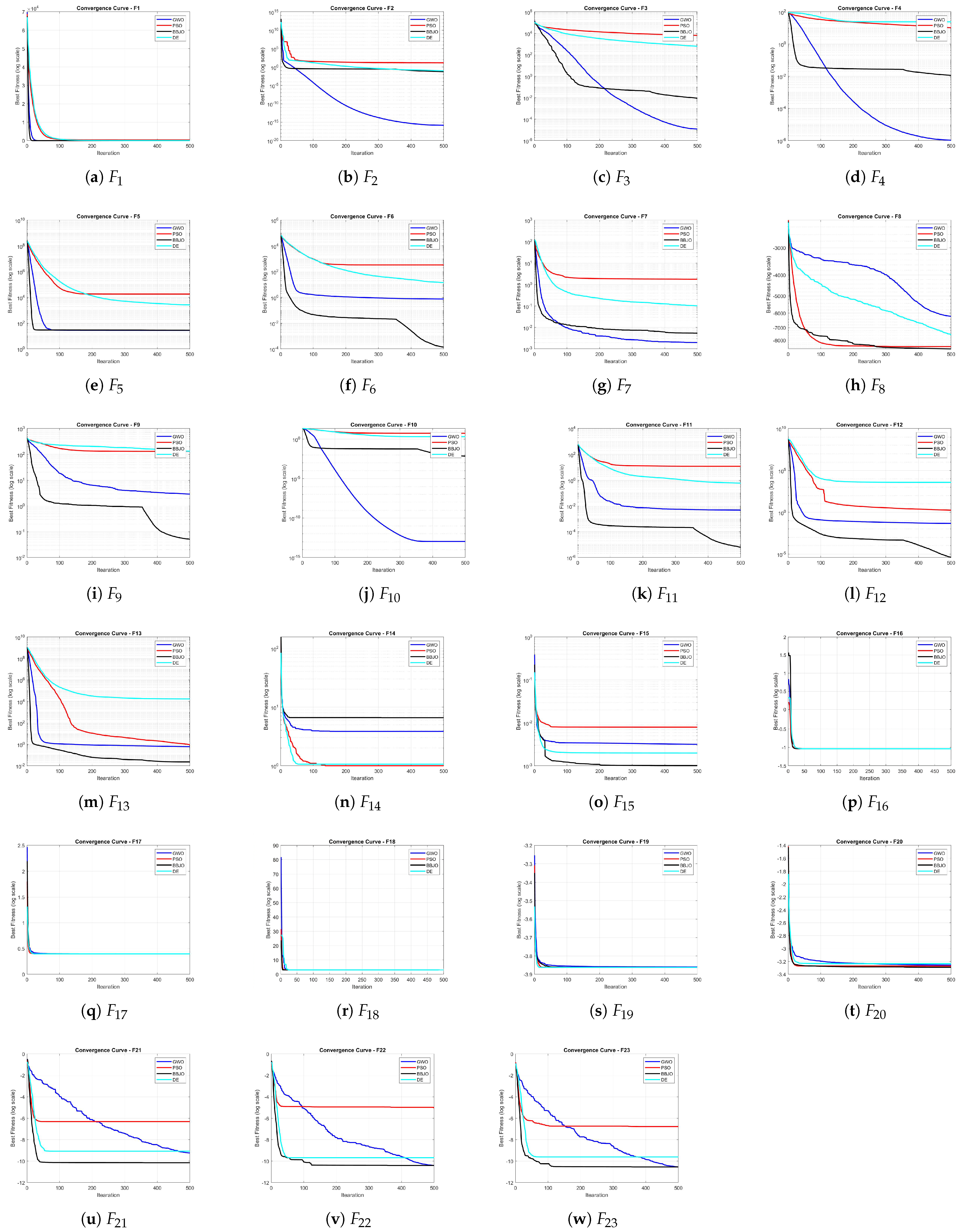
The optimization trajectories across all 23 benchmark functions are consolidated in Figure 4. On the unimodal landscapes ($F_1–F_7$), BBJO exhibits a steep initial descent within the first 50 iterations, outperforming the flatter convergence paths of PSO and DE. For the standard multimodal problems ($F_8–F_{13}$), BBJO’s curves display sharp, step-like drops that indicate successful local optima avoidance triggered by its heavy-tailed Lévy flights, while GWO and PSO prematurely plateau. Finally, on the fixed-dimension surfaces ($F_{14}–F_{23}$), BBJO consistently hits the exact global theoretical minimum on the Shekel functions ($F_{21}–F_{23}$), maintaining a perfectly stable convergence envelope across all 30 independent trials.

7.2. Optimal Design of Fuzzy Controllers: Experimentation

7.2.1. Experimental Setup

Two Mamdani FIS applications benchmark the performance of BBJO against 13 established meta-heuristic solvers [64,65]. These industrial calibration tasks tune scaling and membership parameters, modeling them as highly non-linear, constrained optimization problems. Each competitor minimizes a multi-component objective function $J\left(\mathbf{X}\right)$ over a discrete simulation horizon:

$$\underset{\mathbf{X}\in {\mathbb{R}}^D}{min}J\left(\mathbf{X}\right)={\mathsf{\Phi }}_{\mathrm{precision}}\left(\mathbf{X}\right)+\lambda ·{\mathsf{\Psi }}_{\mathrm{transient}}\left(\mathbf{X}\right)$$

(23)

where $\mathbf{X}$ represents the decision vector of tunable fuzzy parameters ($D=22$ for the speed regulator, $D=15$ for the smart oven). The term ${\mathsf{\Phi }}_{\mathrm{precision}}$ minimizes tracking or steady-state error, while ${\mathsf{\Psi }}_{\mathrm{transient}}$ penalizes transient dynamics like mechanical jerk or thermal overshoot. The coefficient $\lambda$ scales these components.

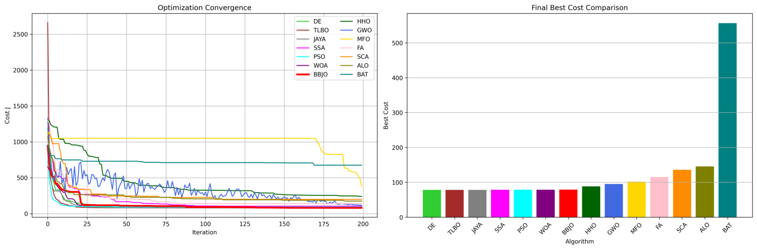
In this study, robustness means run-to-run consistency under random population initialization: each of the 14 solvers is executed for 30 independent trials with different random seeds, and robustness is quantified as the standard deviation of the final $J\left(\mathbf{X}\right)$ across these trials. A low standard deviation indicates that an algorithm reliably converges to a similar-quality solution regardless of its random starting population, which is the relevant notion of reliability for automated re-tuning pipelines. This work does not evaluate robustness to external plant-model uncertainty (e.g., sensor noise, actuator delay, or parameter drift in the vehicle or oven dynamics); We do not evaluate this here and note it as a limitation of the current study.

All 14 algorithms run with a standardized population $N=50$ over 200 iterations. For BBJO, a non-linear parabolic energy decay $E=2(1-{(it/iters)}^2)$ governs the transition between exploration and exploitation. The algorithm switches from heavy-tailed Lévy flights for wide spatial exploration to localized Gaussian sniffing for fine-grained refinement. Throughout the optimization, a sorting and clipping repair operator enforces the ordering constraint $P_i\le P_{i+1}$ across all membership function peaks, guaranteeing physical and linguistic validity.

7.2.2. Autonomous Vehicle Speed Regulator FIS

The speed regulator optimization involves a non-smooth, 22-dimensional search space combining ITAE and vehicle jerk. For automotive safety, run-to-run reliability during automated re-tuning outweighs a single, isolated optimum.

Table 9. Performance and improvement vs. BAT for the speed regulator FIS (30 runs).

Alg.	Best	Mean	Std	vs. BAT
DE	78.32	83.46	9.55	85.92%
TLBO	78.40	78.96	0.71	85.91%
Jaya	78.49	79.07	0.30	85.89%
SSA	78.73	103.84	22.42	85.85%
PSO	78.87	92.46	12.89	85.82%
WOA	78.90	83.51	5.62	85.82%
BBJO	79.21	80.35	1.28	85.76%
HHO	88.60	240.14	151.10	84.08%
GWO	95.10	116.65	12.51	82.91%
MFO	101.63	379.83	229.47	81.73%
FA	115.44	139.64	17.06	79.25%
SCA	136.12	198.14	64.35	75.53%
ALO	145.56	174.58	15.44	73.84%
BAT	556.34	674.89	80.25	0.00%

evaluates this operational consistency using the best cost and standard deviation over 30 independent trials.

BBJO demonstrates exceptional robustness here, achieving the lowest variance ($\mathrm{std}=1.28$, mean = 80.35) among all 14 competitors. Conversely, PSO reaches a low peak cost (78.87) but exhibits a tenfold increase in variability ($\mathrm{std}=12.89$). This indicates highly unpredictable tuning cycles, an instability that worsens with SSA (22.42) and HHO (151.10). For safety-critical longitudinal control, such fluctuations are unacceptable; they risk sudden tracking degradation. While DE (78.32), TLBO (78.40), and Jaya (78.49) form the absolute peak tier below the 78.50 threshold, BBJO remains highly competitive (79.21), finishing within 1.2 units of the global optimum. Other baselines simply stagnate on suboptimal plateaus well outside this competitive zone.

Figure 5 corroborates these findings. BBJO exhibits a steady descent and stabilizes around iteration 75. Meanwhile, PSO oscillates heavily and SSA shows a wide variance band. Weak optimizers like BAT, SCA, and ALO rapidly flatten out and stagnate early. When agents hit the massive flat regions of the fuzzy logic landscape, BBJO deploys heavy-tailed Lévy flights to break the deadlock. These sudden, long-range jumps give the population the exact momentum needed to escape local traps.

7.2.3. Smart Oven Temperature Regulation FIS

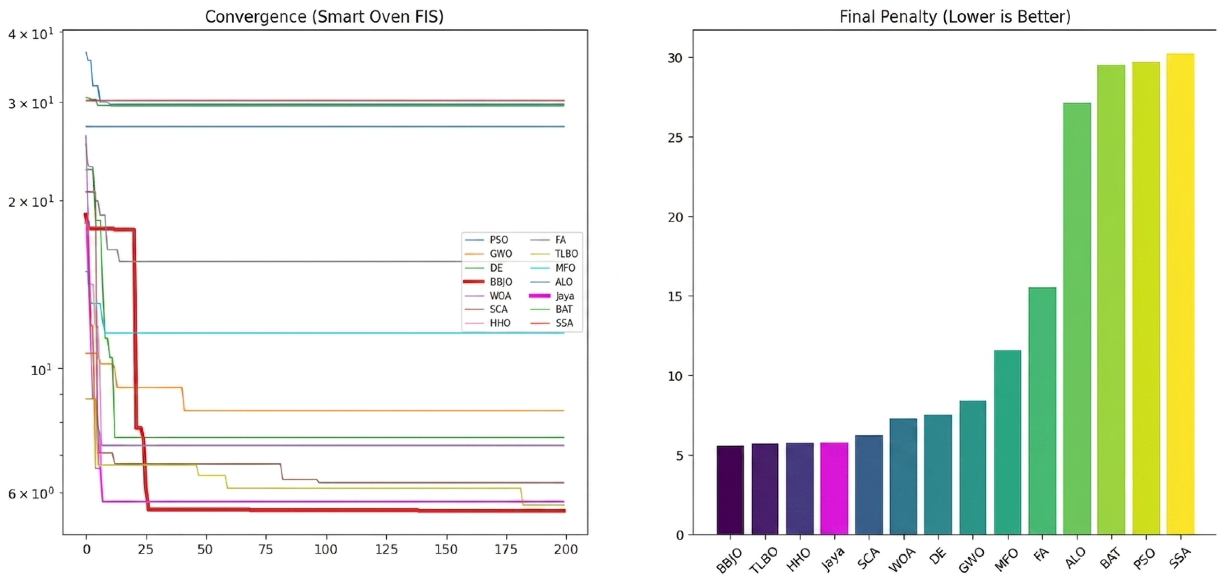
The smart oven optimization presents a non-linear fitness landscape with severe local optima, as illustrated in Figure 6. Solvers like PSO and ALO stagnate immediately in these areas. In contrast, BBJO maintains strong search mobility during iterations 10–25, bypassing local traps to reach the lowest final cost of 5.55 (

Table 10. Final costs and improvement relative to PSO for the smart oven FIS.

Algorithm	Final Cost	Improv. vs. PSO
BBJO	5.55	81.30%
TLBO	5.68	80.84%
HHO	5.77	80.57%
Jaya	5.77	80.57%
SCA	6.24	78.98%
WOA	7.27	75.50%
DE	7.52	74.67%
GWO	8.40	71.70%
MFO	11.56	61.04%
FA	15.52	47.70%
ALO	27.08	8.73%
BAT	29.49	0.62%
PSO	29.67	0.00%
SSA	30.19	−1.76%

). This result outperforms the second-best solver, TLBO (5.68), by 2.3% and reduces the PSO penalty (29.67) by 81.30%. This high accuracy stems directly from the Quadratic Prey Refinement operator, which minimizes steady-state errors much better than the rigid linear updates of GWO or PSO.

7.2.4. Global Discussion

BBJO shows a reliable and robust behavioral profile across both industrial applications. In the smart oven case, it secures the lowest absolute penalty score of 5.55. For the speed regulator task, it reaches a highly competitive mean cost of 80.35, marking a 13.1% improvement over standard PSO. At the same time, it provides the lowest standard deviation in the entire test field (1.28). This performance makes BBJO ten times more stable than PSO and a hundred times more predictable than HHO.

This double advantage comes directly from the structural design of BBJO. The parabolic energy decay mechanism maintains global search mobility longer than standard linear methods. This characteristic keeps the mean costs highly competitive across independent runs, even if a competing method occasionally identifies a lower isolated optimum. Additionally, fuzzy logic control surfaces contain massive flat zones where algorithms typically stall. When agents hit these regions, BBJO deploys heavy-tailed Lévy flights to break the deadlock. These sudden, long-range jumps provide the exact momentum needed to escape local traps, preventing the heavy stagnation that ruins methods like BAT, SCA, ALO, and MFO.

The baseline methods highlight a clear limitation in the remaining solvers. Algorithms like BAT, ALO, SCA, and MFO consistently fail to locate the global optimum in both engineering benchmarks. Their main design weakness stems from a lack of long-range displacement steps combined with a rigid linear decay. Consequently, they suffer from premature stagnation, spending their iteration budget inside suboptimal local valleys before they can identify the global search zone.

For physical implementations, control engineers value mean performance across deployments over single, isolated optimization runs. A tuning algorithm that delivers a tight mean of 80.35 with a standard deviation of 1.28 is practically superior to a method averaging 92.46 with a deviation of 12.89. This predictability ensures that the physical controller operates safely and reliably every time the system triggers an automated re-tuning cycle.

8. Conclusions

This paper presented the Black-Backed Jackal Optimization (BBJO) meta-heuristic, inspired by the opportunistic foraging and stamina dynamics of Lupulella mesomelas. By integrating a non-linear parabolic energy decay with adaptive Lévy flights, the algorithm achieves a robust balance between exploration and exploitation. Benchmark evaluations across 23 classical functions confirmed its capacity to bypass local optima. Specifically, BBJO achieved mean errors two orders of magnitude lower than PSO on unimodal surfaces ($F_1,F_6$), prevented premature convergence on high-dimensional multimodal topologies ($F_8,F_9,F_{11}–F_{13}$), and consistently reached the exact theoretical minima with zero variance on Shekel functions ($F_{21}–F_{23}$).

Practical validation on two industrial fuzzy control tasks demonstrated the algorithm’s field readiness. For the smart oven system, BBJO secured the lowest overall penalty (5.55), outperforming TLBO by 2.3% and PSO by 81.30%. In the autonomous vehicle speed regulation test, BBJO established superior run-to-run consistency with the lowest standard deviation (1.28) and a 13.1% mean cost reduction over PSO. These metrics show that BBJO provides the deterministic stability necessary for safety-critical industrial loops. Future work will adapt BBJO for multi-objective challenges, focusing on the tradeoff between ITAE and overshoot, while shifting from simulation to real-time embedded hardware validation.

References

1. Zadeh, L.A. Fuzzy sets. Inf. Control 1965, 8, 338–353. [Google Scholar] [CrossRef] [Scilit]
2. Mamdani, E.H.; Assilian, S. An experiment in linguistic synthesis with a fuzzy logic controller. Int. J. Man-Mach. Stud. 1975, 7, 1–13. [Google Scholar] [CrossRef] [Scilit]
3. El Moutaouakil, K.; Cheggour, M.; Chellak, S.; Baizri, H. Metaheuristics optimization algorithm to an optimal Moroccan diet. In Proceedings of the 2021 7th Annual International Conference on Network and Information Systems for Computers (ICNISC), Guiyang, China, 23–25 July 2021; IEEE: New York, NY, USA, 2021; pp. 364–368. [Google Scholar]
4. Kar, I.; Behera, L. Hybrid soft computing strategies for the control of nonlinear systems: A review. Theor. Comput. Sci. 2014, 529, 107–127. [Google Scholar] [CrossRef] [Scilit]
5. Bonissone, P.P.; Badami, V.; Chiang, K.H.; Khedkar, P.S.; Marcelle, K.; Schutten, M. Industrial applications of fuzzy logic at General Electric. Proc. IEEE 1995, 84, 437–449. [Google Scholar]
6. Agrawal, S.; Kumar, R. A comprehensive review on meta-heuristic algorithms for solving optimization problems: Applications, challenges and future prospects. Complex Intell. Syst. 2021, 7, 2221–2245. [Google Scholar]
7. Precup, R.E.; David, R.C. Nature-Inspired Optimization Algorithms for Fuzzy Controlled Servo Systems; Butterworth-Heinemann: Oxford, UK, 2019. [Google Scholar]
8. Rakshit, S.M.; Das, N.K. Fuzzy Logic Based Speed Control of Autonomous Vehicles for Safe Distance Maintenance. Int. J. Eng. Res. 2021, 10, 112–118. [Google Scholar] [CrossRef] [Scilit]
9. Hossain, M.J. Design of a Fuzzy Temperature Controller for Electric Furnaces with Improved Step Response. Control Eng. Pract. 2020, 102, 104500. [Google Scholar] [CrossRef] [Scilit]
10. Viswanathan, G.M.; Buldyrev, S.V.; Havlin, S.; da Luz, M.; Raposo, E.; Stanley, H.E. Optimizing the success of random searches. Nature 1999, 401, 911–914. [Google Scholar] [CrossRef] [Scilit] [PubMed]
11. Loveridge, A.J.; Macdonald, D.W. Behavioural ecology and niche segregation in a sympatric canid community. J. Zool. 2002, 258, 123–131. [Google Scholar] [CrossRef] [Scilit]
12. Wolpert, D.H.; Macready, W.G. No Free Lunch theorems for optimization. IEEE Trans. Evol. Comput. 1997, 1, 67–82. [Google Scholar] [CrossRef] [Scilit]
13. Holland, J.H. Adaptation in Natural and Artificial Systems: An Introductory Analysis with Applications to Biology, Control, and Artificial Intelligence; MIT Press: Cambridge, MA, USA, 1992. [Google Scholar]
14. Goldberg, D.E. Genetic Algorithms in Search, Optimization and Machine Learning; Addison Welssey Publishing Company: Reading, MA, USA, 1989. [Google Scholar]
15. Storn, R.; Price, K. Differential evolution—A simple and efficient heuristic for global optimization over continuous spaces. J. Glob. Optim. 1997, 11, 341–359. [Google Scholar] [CrossRef] [Scilit]
16. Simon, D. Biogeography-based optimization. IEEE Trans. Evol. Comput. 2008, 12, 702–713. [Google Scholar] [CrossRef] [Scilit]
17. Karaboga, D.; Basturk, B. A powerful and efficient algorithm for numerical function optimization: Artificial bee colony (ABC) algorithm. J. Glob. Optim. 2007, 39, 459–471. [Google Scholar] [CrossRef] [Scilit]
18. Reynolds, R.G. An introduction to cultural algorithms. In Proceedings of the Third Annual Conference on Evolutionary Programming, River Edge, NJ, USA, 24–26 February 1994; World Scientific: Singapore, 1994; pp. 131–139. [Google Scholar]
19. Hansen, N.; Ostermeier, A. Completely derandomized self-adaptation in evolution strategies. Evol. Comput. 2001, 9, 159–195. [Google Scholar] [CrossRef] [Scilit] [PubMed]
20. Rashedi, E.; Nezamabadi-Pour, H.; Saryazdi, S. GSA: A gravitational search algorithm. Inf. Sci. 2009, 179, 2232–2248. [Google Scholar] [CrossRef] [Scilit]
21. Hashim, F.A.; Hussain, K.; Houssein, E.H.; Mabrouk, M.S.; Al-Atabany, W. Archimedes optimization algorithm: A new metaheuristic algorithm for solving optimization problems. Appl. Intell. 2021, 51, 1531–1551. [Google Scholar]
22. Mirjalili, S. SCA: A sine cosine algorithm for solving optimization problems. Knowl.-Based Syst. 2016, 96, 125–137. [Google Scholar] [CrossRef] [Scilit]
23. Mirjalili, S.; Mirjalili, M.M.; Hatamlou, A. Multi-verse optimizer: A nature-inspired algorithm for global optimization. Neural Comput. Appl. 2015, 27, 495–513. [Google Scholar] [CrossRef] [Scilit]
24. Faramarzi, A.; Heidari, A.A.; Stephens, B.; Mirjalili, S. Equilibrium optimizer: A novel optimization algorithm. Knowl.-Based Syst. 2020, 191, 105190. [Google Scholar] [CrossRef] [Scilit]
25. Hashim, F.A.; Hussain, K.; Houssein, E.H.; Mabrouk, M.S.; Al-Atabany, W. Henry gas solubility optimization: A novel physics-based algorithm. Future Gener. Comput. Syst. 2019, 101, 646–667. [Google Scholar] [CrossRef] [Scilit]
26. Kaveh, A.; Dadras, A. A novel meta-heuristic optimization algorithm: Thermal exchange optimization. Adv. Eng. Softw. 2016, 110, 69–84. [Google Scholar] [CrossRef] [Scilit]
27. Talatahari, S.; Azizi, M. Crystal Structure Algorithm (CryStAl): A New Nature-Inspired Meta-Heuristic Optimization Method. IEEE Access 2021, 9, 17744–17761. [Google Scholar] [CrossRef] [Scilit]
28. Kennedy, J.; Eberhart, R. Particle swarm optimization. In Proceedings of the ICNN’95—International Conference on Neural Networks, Perth, WA, Australia, 27 November–1 December 1995; IEEE: New York, NY, USA, 1995; Volume 4, pp. 1942–1948. [Google Scholar]
29. Mirjalili, S.; Mirjalili, M.; Lewis, A. Grey Wolf Optimizer. Adv. Eng. Softw. 2014, 69, 46–61. [Google Scholar] [CrossRef] [Scilit]
30. Mirjalili, S.; Lewis, A. The whale optimization algorithm. Adv. Eng. Softw. 2016, 95, 51–67. [Google Scholar] [CrossRef] [Scilit]
31. Mirjalili, S.; Gandomi, A.H.; Mirjalili, M.Z.; Saremi, S.; Faris, H.; Mirjalili, S.M. Salp Swarm Algorithm: A bio-inspired optimizer for engineering design problems. Adv. Eng. Softw. 2017, 114, 163–191. [Google Scholar] [CrossRef] [Scilit]
32. Xue, J.; Shen, B. A novel sparrow search algorithm. Syst. Sci. Control Eng. 2020, 8, 22–34. [Google Scholar] [CrossRef] [Scilit]
33. Yang, X.S. Firefly algorithms for multimodal optimization. In Proceedings of the International Symposium on Stochastic Algorithms, Sapporo, Japan, 26–28 October 2009; Springer: Berlin/Heidelberg, Germany, 2009; pp. 169–178. [Google Scholar]
34. Fister, I.; Fister, I., Jr.; Yang, X.S.; Brest, J. A comprehensive review of firefly algorithms. Swarm Evol. Comput. 2013, 13, 34–46. [Google Scholar] [CrossRef] [Scilit]
35. Heidari, A.A.; Mirjalili, S.; Faris, H.; Aljarah, I.; Mafarja, M.; Chen, H. Harris hawks optimization: Algorithm and applications. Future Gener. Comput. Syst. 2019, 97, 849–872. [Google Scholar] [CrossRef] [Scilit]
36. Xue, J.; Shen, B. Dung beetle optimizer: A new meta-heuristic algorithm for digital image watermarking and optimization. J. Supercomput. 2023, 79, 12305–12336. [Google Scholar]
37. Abdel-Basset, M.; Mohamed, R.; Jameel, M.; Abu-Zied, M.S. Crested Porcupine Optimizer: A new nature-inspired metaheuristic algorithm. Knowl.-Based Syst. 2024, 284, 111257. [Google Scholar] [CrossRef] [Scilit]
38. Zhao, W.; Wang, L.; Mirjalili, S. Artificial hummingbird algorithm: A new bio-inspired optimizer with its engineering applications. Comput. Methods Appl. Mech. Eng. 2022, 388, 114194. [Google Scholar] [CrossRef] [Scilit]
39. Abdel-Basset, M.; Mohamed, R.; Zidan, M.; Jameel, M.; Abouhawwash, M. Mantis Search Algorithm: A novel bio-inspired algorithm for global optimization and engineering design problems. Comput. Methods Appl. Mech. Eng. 2023, 415, 116200. [Google Scholar] [CrossRef] [Scilit]
40. Abdel-Basset, M.; Mohamed, R.; Azeem, S.A.; Jameel, M.; Abouhawwash, M. Nutcracker optimization algorithm: A new nature-inspired metaheuristic algorithm for solving continuous and discrete optimization problems. Knowl.-Based Syst. 2023, 262, 110248. [Google Scholar] [CrossRef] [Scilit]
41. Trojovská, E.; Dehghani, M.; Trojovskỳ, P. Zebra optimization algorithm: A new bio-inspired optimization algorithm for solving optimization algorithm. IEEE Access 2022, 10, 49445–49473. [Google Scholar] [CrossRef] [Scilit]
42. Pavlyukevich, I. Lévy flights, Lévy fractional diffusion and genetic algorithms. J. Comput. Phys. 2007, 226, 1830–1844. [Google Scholar] [CrossRef] [Scilit]
43. Yang, X.S. Nature-Inspired Metaheuristic Algorithms; Luniver Press: Frome, UK, 2010. [Google Scholar]
44. Chopra, N.; Ansari, M.A. Golden jackal optimization: A novel nature-inspired optimizer for engineering problems. Expert Syst. Appl. 2022, 191, 116248. [Google Scholar]
45. Abdollahzadeh, B.; Gharehchopogh, F.R.; Mirjalili, S. African vultures optimization algorithm: A new nature-inspired metaheuristic algorithm for global optimization problems. Comput. Ind. Eng. 2021, 158, 107408. [Google Scholar] [CrossRef] [Scilit]
46. Rao, R.V.; Savsani, V.J.; Vakharia, D.P. Teaching–learning-based optimization: A novel method for constrained mechanical design optimization problems. Comput.-Aided Des. 2011, 43, 303–315. [Google Scholar] [CrossRef] [Scilit]
47. Rao, R.V. Jaya: A simple and new optimization algorithm for solving constrained and unconstrained optimization problems. Int. J. Ind. Eng. Comput. 2016, 7, 19–34. [Google Scholar] [CrossRef] [Scilit]
48. Mirjalili, S. Moth-flame optimization algorithm: A novel nature-inspired heuristic paradigm. Knowl.-Based Syst. 2015, 89, 228–249. [Google Scholar] [CrossRef] [Scilit]
49. Mirjalili, S. The ant lion optimizer. Adv. Eng. Softw. 2015, 83, 80–98. [Google Scholar] [CrossRef] [Scilit]
50. Yang, X.S. A new metaheuristic bat-inspired algorithm. In Nature Inspired Cooperative Strategies for Optimization (NICSO 2010); Studies in Computational Intelligence; González, J.R., Pelta, D.A., Cruz, C., Terrazas, G., Krasnogor, N., Eds.; Springer: Berlin/Heidelberg, Germany, 2010; Volume 284, pp. 65–74. [Google Scholar]
51. Kaunda, S.; Skinner, J. Black-backed jackal diet at Mokolodi nature reserve, Botswana. Afr. J. Ecol. 2003, 41, 39–46. [Google Scholar] [CrossRef] [Scilit]
52. Mitchell, C. Jackals—Facts, Characteristics, History, Habitat, Lifespan, and More! World Animal Foundation: Dover, DE, USA, 2023; Available online: https://worldanimalfoundation.org (accessed on 1 May 2026).
53. Koepfli, K.P.; Pollinger, J.; Godinho, R.; Robinson, J.; Lea, A.; Hendricks, S.; Schweizer, R.M.; Thalmann, O.; Silva, P.; Fan, Z.; et al. Genome-wide evidence reveals that African and Eurasian golden jackals are distinct species. Curr. Biol. 2015, 25, 2158–2165. [Google Scholar] [CrossRef] [Scilit] [PubMed]
54. Atickem, A.; Stenseth, N.C.; Drouilly, M.; Bock, S.; Roos, C.; Zinner, D. Deep divergence among mitochondrial lineages in African jackals. Zool. Scr. 2018, 47, 1–8. [Google Scholar]
55. Moehlman, P.D. Social organization in jackals. Am. Sci. 1987, 75, 366–375. [Google Scholar]
56. Mech, L.D. Alpha status, dominance, and division of labor in wolf packs. Can. J. Zool. 1999, 77, 1196–1203. [Google Scholar] [CrossRef]
57. Gorman, M.L.; Mills, M.G.; Raath, J.P.; Speakman, J.R. High hunting costs make African wild dogs vulnerable to kleptoparasitism by hyaenas. Nature 1998, 391, 479–481. [Google Scholar] [CrossRef] [Scilit]
58. Van der Merwe, J. The Ecology of the Black-Backed Jackal in the Royal Natal National Park; University of Natal: Durban, South Africa, 1981. [Google Scholar]
59. Reynolds, A.; Rhodes, C. Lévy flights in nature: Are they regional or universal? J. Theor. Biol. 2009, 259, 447–456. [Google Scholar] [CrossRef] [Scilit] [PubMed]
60. Hiscocks, K.; Perrin, M. The foraging ecology of the black-backed jackal in the Central Namib Desert. S. Afr. J. Wildl. Res. 1988, 18, 81–86. [Google Scholar]
61. Mantegna, R.N. Fast, accurate algorithm for numerical simulation of Levy stable stochastic processes. Phys. Rev. E 1994, 49, 4677. [Google Scholar] [CrossRef] [Scilit]
62. Rudolph, G. Convergence Properties of Evolutionary Algorithms; Kovac: Hamburg, Germany, 1997. [Google Scholar]
63. Charroud, A.; El Moutaouakil, K.; Palade, V.; Yahyaouy, A.; Onyekpe, U.; Eyo, E.U. Localization and mapping for self-driving vehicles: A survey. Machines 2024, 12, 118. [Google Scholar] [CrossRef] [Scilit]
64. El Ouissari, A.; El Moutaouakil, K.; Baizri, H.; Chellak, S. Intelligent local search for an optimal control of diabetic population dynamics. Math. Model. Comput. Simul. 2022, 14, 1051–1071. [Google Scholar] [CrossRef] [Scilit]
65. El Moutaouakil, K.; Ahourag, A.; Chakir, S.; Kabbaj, Z.; Chellack, S.; Cheggour, M.; Baizri, H. Hybrid firefly genetic algorithm and integral fuzzy quadratic programming to an optimal Moroccan diet. Math. Model. Comput. 2023, 10, 338–350. [Google Scholar] [CrossRef] [Scilit]
Figure 1. Behavioral repertoire of Lupulella mesomelas. Source: Mitchell (2023), World Animal Foundation [52]. (a) Cooperative pair hunting: pair-based leadership modelled in BBJO. (b) Small-group foraging with one individual maintaining vigilance. (c) Opportunistic scavenging: biological basis for Equation (13).
Algorithms 19 00566 g001
Figure 2. Phylogenetic tree of wolf-like canids. The black-backed jackal diverged from the main Canis lineage at ≈5.2 Ma; fossil evidence shows the species has remained morphologically stable since ≈2.5 Ma.
Algorithms 19 00566 g002
Figure 3. Structural Mapping of Biological Inspiration to BBJO Operators. Biological behaviors are mapped to mathematical search operators. The transition between them is controlled by | E | . The precision-hunting refinement mirrors the low-stamina, targeted hunting mode described in [58].
Algorithms 19 00566 g003
Figure 4. Convergence profiles across all benchmark landscapes: unimodal ( F 1 F 7 ), standard multimodal ( F 8 F 13 ), and fixed-dimension multimodal ( F 14 F 23 ) functions.
Algorithms 19 00566 g004
Figure 5. Optimization criterion: the FIS objective cost J ( X ) of Equation (23), combining tracking precision and jerk-based transient penalty. Left: evolution of the best J ( X ) found so far versus iteration count for all 14 solvers. Right: final best J ( X ) reached by each algorithm after 200 iterations, averaged over 30 independent trials (lower is better).
Algorithms 19 00566 g005
Figure 6. Optimization criterion: the FIS objective cost J ( X ) of Equation (23), here combining steady-state temperature error and thermal-overshoot penalty. Left: evolution of the best J ( X ) found so far versus iteration count for all 14 solvers. Right: final best J ( X ) (penalty) reached by each algorithm, averaged over 30 independent trials (lower is better).
Algorithms 19 00566 g006