ECPD-SG: An Emotion-Aware Contrastive Prototype Algorithm for Change Point Detection in Dynamic Social Graphs

Abstract

Change point detection in dynamic social graphs aims to identify significant transitions in evolving interaction patterns. The task is particularly challenging due to sparse and noisy interactions and frequent user turnover, while the existing methods largely overlook the semantic and emotional signals in user-generated content by focusing primarily on structural changes. To address these limitations, this paper proposes ECPD-SG, an emotion-aware contrastive prototype learning algorithm for unsupervised change point detection in dynamic social graphs. ECPD-SG constructs emotion-aware graph snapshots by integrating textual and affective features into node representations and recalibrating interaction weights through emotion-aware attention. It then summarizes temporal node representations into adaptive prototypes and models their evolution using optimal-transport-based alignment and contrastive learning. Change points are detected from prototype-level shift scores with an adaptive CUSUM decision rule. Experiments on real-world dynamic social graph datasets show that ECPD-SG achieves competitive or superior performance over representative baselines, while ablation and sensitivity analyses verify the effectiveness of its key components.

1. Introduction

Text-rich social interaction systems continuously capture how large populations communicate, interact, and respond to real-world events, generating dynamic social graphs that evolve in both structure and content. When significant events occur, these graphs undergo abrupt transitions in communication patterns and community organization, marking critical boundaries between qualitatively distinct phases of online social activity. Detecting such transitions, referred to as change points, is of broad practical relevance, with applications in event tracking [1], public opinion analysis [2], and misinformation detection [3]. Compared with general dynamic graphs, dynamic social graphs contain not only time-varying interaction structures but also rich user-generated textual content that carries semantic information.

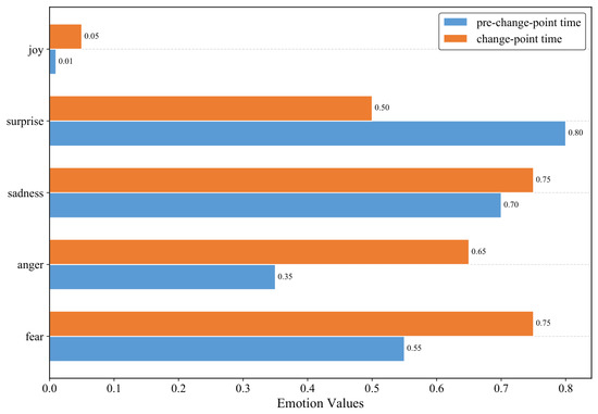
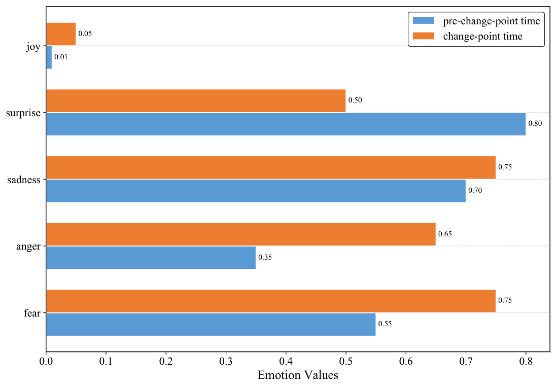
A key observation motivating this work is that change points in dynamic social graphs are often accompanied by pronounced shifts in the emotional composition of user-generated content. Since user posts are associated with users and their interactions in the graph, the emotional signals embedded in such content constitute an important part of the evolving graph state rather than merely external annotations. Figure 1 illustrates this through the Charlie Hebdo event: compared with the pre-change-point period, the change-point period exhibits a clear redistribution of comment-level emotional categories, with anger, fear, and sadness becoming more prominent while surprise declines. This observation suggests that emotional signals provide a complementary perspective to graph topology for characterizing change points.

Figure 1. Distribution of emotional categories in user-generated content before and at the change point during the Charlie Hebdo event.

Nevertheless, detecting change points from node-level representations remains challenging because the node space in dynamic social graphs is often unstable. Users may appear or disappear across snapshots, while local interactions and user-generated content are frequently sparse, noisy, and sensitive to short-term fluctuations. Directly comparing individual nodes may therefore amplify transient local changes and obscure broader social transitions. A more principled approach is to characterize each snapshot through latent group patterns, where users with similar interaction patterns, textual semantics, and emotional states are summarized together into compact prototype representations. Since important social transitions often manifest as reorganizations of user groups rather than isolated node-level variations, prototype-based representations provide a more robust basis for change point detection in dynamic social graphs.

The existing methods for change point detection in dynamic graphs can be roughly divided into two groups. The first group identifies changes from explicit structural signals, such as Laplacian spectra, community structures, and node centrality [4,5,6]. The second group learns node-level or graph-level representations and detects changes through embedding deviations, graph similarities, or reconstruction errors [7,8,9,10]. Despite their effectiveness, these methods are less suited to dynamic social graphs, where user posts provide not only textual semantics but also affective signals that reflect changes in online discussions. Most of the existing approaches either focus on structural variation or treat node attributes as generic features, without distinguishing the emotional dimension embedded in user-generated content. Moreover, their node-level or snapshot-level comparisons often overlook stable group-level patterns, limiting their ability to characterize social transitions that involve structural, semantic, and emotional changes.

To address these limitations, we propose ECPD-SG, an emotion-aware contrastive prototype learning algorithm for unsupervised change point detection in dynamic social graphs. ECPD-SG first constructs emotion-aware graph snapshots by integrating textual semantics and affective representations into node features and interaction weights. It then applies a temporal graph encoder to learn evolving node representations and summarizes each snapshot into a set of adaptive prototypes, where each prototype represents a dominant group-level graph state. Prototype evolution is modeled through optimal-transport-based alignment and contrastive learning, which preserves temporal consistency while remaining sensitive to genuine transitions. Finally, change points are detected from prototype-level shift scores using an adaptive decision rule. The main contributions of this paper are summarized as follows:

• We formulate change point detection in dynamic social graphs as an unsupervised prototype-based graph sequence detection problem and propose ECPD-SG, an emotion-aware contrastive prototype learning algorithm for identifying group-level state transitions.
• We design an emotion-aware graph snapshot construction strategy that integrates textual semantics and affective signals into node representations and recalibrates observed interaction weights through emotion-aware attention.
• We introduce an optimal-transport-aligned contrastive prototype dynamics module to summarize each snapshot into adaptive prototypes and model their temporal evolution for robust change point scoring.
• Our extensive experiments on real-world dynamic social graph datasets demonstrate that ECPD-SG consistently outperforms competitive baselines, while our ablation studies further verify the effectiveness of emotion-aware graph modeling and contrastive prototype dynamics.

2. Related Work

2.1. Change Point Detection in Dynamic Graphs

The existing methods for change point detection in dynamic graphs fall into two broad categories: statistical approaches and representation-learning approaches. Statistical approaches detect change points by monitoring explicit graph statistics, structural summaries, or probabilistic changes computed from graph snapshots. Early studies mainly formulated dynamic graph change detection as a statistical testing problem over evolving network structures. GHRG [11] detects changes in the large-scale structure of evolving networks by fitting hierarchical random graph models and performing Bayesian hypothesis testing between consecutive temporal segments. To improve efficiency under the snapshot model, EdgeMonitoring [12] estimates edge-probability distributions within sliding windows and compares their changes across time, providing a scalable likelihood-based solution for dynamic social networks. Later methods have further enriched the structural summaries used for detection. CICPD [6] characterizes each snapshot through node-importance distributions and community profiles, and it identifies change points by tracking variations among clustered snapshot representations. LAD [4] introduces a spectral view by representing each snapshot with graph Laplacian eigenvalues, allowing both short-term and long-term structural variations to be captured through temporal windows. MultiLAD [5] extends this Laplacian-based idea to single-view and multi-view dynamic graphs, making it applicable to graph sequences with multiple relational views. Although effective for detecting topological changes, these methods mainly rely on explicit structural summaries, making them less suitable for dynamic social graphs where user-generated posts carry important textual semantics and emotional signals.

Representation-learning approaches learn node-level, graph-level, or latent representations of dynamic graphs and then detect change points from temporal inconsistencies in the learned space: s-GNN [8] formulates online change point detection as a graph similarity learning problem, using graph neural networks to learn a similarity function between graph snapshots for real-time structural change detection; CPDlatent [9] adopts a decoder-only latent space model to learn low-dimensional graph representations and uses Group Fused Lasso regularization to identify structural changes in graph sequences; CD-HADG [10] extends change point detection to highly attributed dynamic graphs by estimating graph modularity with graph neural networks, allowing the model to capture changes in both graph structure and high-dimensional node attributes. More broadly, optimization-based approaches to network alignment, including nature-inspired meta-heuristic methods [13], provide a general perspective on how graph structures can be compared and matched, which is relevant to the prototype alignment step in our framework.

Although these methods improve dynamic graph modeling beyond hand-crafted structural statistics, they are mostly designed for general dynamic graphs and provide limited modeling of user-generated textual and emotional content. This motivates the need to consider emotion-aware social graph representation learning for content-rich dynamic social graphs.

2.2. Emotion-Aware Social Graph Representation Learning

Emotion modeling has received growing attention in social graph analysis, as user-generated content carries affective signals that reflect collective responses to social events and interactions [14,15,16]. Beyond structural signals, text-based approaches have shown that latent emotional states can be inferred from social media content, including detection of depression-related patterns from user posts [17]. Early work extracts sentiment or emotion features from text and incorporates them into graph-based analysis, demonstrating that emotional information provides useful context for understanding user behavior and network structure [18,19,20]. More recent studies integrate affective signals directly into graph neural networks: emotion-enhanced GNNs jointly encode textual sentiment and graph topology into node representations [21], sequence models combined with sentiment classifiers identify abnormal emotional patterns in crisis-related social media streams [22]. Despite these advances, existing emotion-aware methods mainly focus on sentiment analysis, user behavior modeling, bot detection, or local anomaly detection, and they have not sufficiently explored how emotional information can be integrated into dynamic social graph representations for change point detection.

2.3. Contrastive Learning for Dynamic Graphs

Contrastive learning has been applied to dynamic graphs to improve the robustness and discriminability of temporal node representations. DySubC [23] constructs a subgraph-level contrastive task by sampling temporal subgraphs around target nodes. DyGCL [24] encourages short-term temporal consistency while contrasting long-term inconsistent node pairs. TGAC [25] generates informative contrastive views through temporal graph augmentation. IDOL [26] updates representations incrementally by monitoring topology changes. These methods advance self-supervised learning on dynamic graphs, but they are optimized for node classification or link prediction rather than change point detection, and they operate at the node or subgraph level without modeling group-level graph evolution. In contrast, ECPD-SG applies contrastive learning to prototype dynamics, regularizing the temporally aligned evolution of dynamic prototypes to capture stable group-level patterns and detect structural transitions.

3. Preliminaries

We represent a dynamic social graph as a sequence of temporal snapshots $\mathcal{G}=\{G_1,G_2,\dots ,G_T\}$, where each snapshot is a tuple $G_t=(V_t,E_t,X_t^{\mathrm{text}},X_t^{\mathrm{emo}}).$ Here, $V_t$ is the node set of users, $E_t$ is the edge set of reply interactions, $X_t^{\mathrm{text}}\in {\mathbb{R}}^{n_t\times d}$ are textual semantic features, and $X_t^{\mathrm{emo}}\in {\mathbb{R}}^{n_t\times f}$ are emotional features, with $n_t=\left|V_t\right|$.

Problem Formulation

Given $\mathcal{G}=\{G_1,\dots ,G_T\}$, the goal is to identify a subset $\mathcal{T}*\subseteq \{1,\dots ,T\}$ of time indices at which the graph undergoes significant structural shifts in interaction patterns and node representations. To detect such shifts, we associate each snapshot $G_t$ with a scalar shift score $S_t$, which consists of a short-term adjacent-snapshot component $S_t^{\mathrm{in}}$ and a historical-deviation component $S_t^{\mathrm{out}}$. Here, $S_t^{\mathrm{in}}$ measures short-term changes between adjacent snapshots, and $S_t^{\mathrm{out}}$ measures the deviation of the current snapshot from a recent historical reference window ${\mathcal{H}}_t=\{G_{t-h},\dots ,G_{t-1}\}$. A time index $t\ge t_0$ is declared a change point when $\mathrm{\Psi }(S_{t_0},\dots ,S_t)=1$, where $t_0=max(w,h,w_{\tau })+1$ is the first index with sufficient temporal, historical, and threshold-estimation context, and where $\mathrm{\Psi }$ is a binary decision rule instantiated by a CUSUM statistic with an adaptive threshold, as described in Section 4.3.

4. Methodology

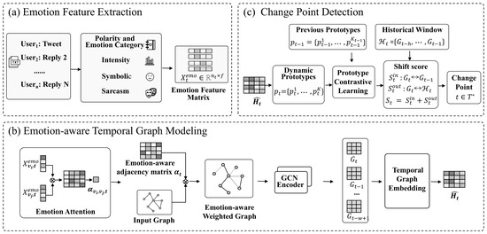
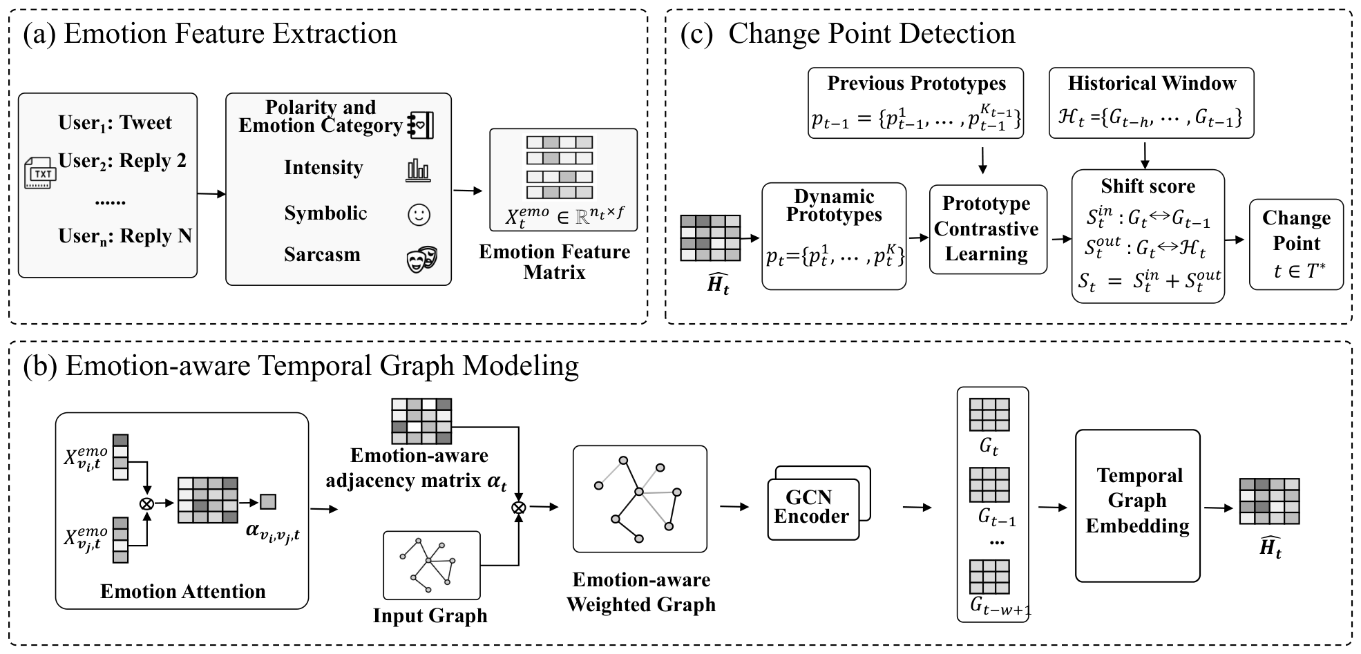
ECPD-SG is designed to detect structural shifts in dynamic social graphs by incorporating textual semantics and emotional signals into temporal graph modeling. As shown in Figure 2, the framework contains three modules: emotion feature extraction, emotion-aware temporal graph modeling, and change point detection. These modules progressively transform user-generated content and interaction structures into temporal node representations, prototype-level dynamics, and final change point decisions.

Figure 2. Overall architecture of ECPD-SG: (a) Emotion feature extraction derives node-level emotion representations from user-generated texts. (b) Emotion-aware temporal graph modeling constructs emotion-aware weighted graphs and encodes their temporal evolution. (c) Contrastive prototype dynamics summarizes temporal node representations into dynamic prototypes and detects change points from prototype shift scores. Gray grid blocks denote matrices or graph snapshots, solid arrows denote the main computational flow, ⊗ denotes emotion-aware structure fusion, and different edge shades in the weighted graph indicate emotion-recalibrated interaction weights.

4.1. Emotion Feature Extraction

For each user node v in snapshot $G_t$, let ${\mathcal{C}}_{v,t}=\{c_1,c_2,\dots ,c_r\}$ denote the textual content associated with v in this snapshot, where $c_j$ is the j-th word. If multiple posts or replies are generated by the same user within the snapshot then they are concatenated in temporal order to form ${\mathcal{C}}_{v,t}$. We extract four groups of emotion features from ${\mathcal{C}}_{v,t}$ and concatenate them into the node-level emotion representation $x_{v,t}^{\mathrm{emo}}$. Stacking the representations of all $n_t$ user nodes gives the emotion feature matrix $X_t^{\mathrm{emo}}\in {\mathbb{R}}^{n_t\times f}$, where f denotes the dimensionality of the final emotion feature vector. Two lexical resources are used in this subsection: a word-level emotion lexicon $\mathcal{D}$, which provides affective relevance scores and emotion intensity scores, and a symbolic sentiment lexicon ${\mathcal{D}}_{\mathrm{sym}}$, which provides polarity scores for symbolic cues such as emojis, kaomojis, and punctuation marks.

4.1.1. Polarity and Emotion Category Features

We use the word-level emotion lexicon $\mathcal{D}$ to derive polarity and emotion category features. Let $\mathcal{P}$ denote the set of polarity classes, including positive, negative, and neutral, and let $\mathcal{M}$ denote the set of emotion categories, such as joy, anger, sadness, and fear. The affective attribute set is defined as $\mathcal{A}=\mathcal{P}\cup \mathcal{M}=\{a_1,a_2,\dots ,a_k\}$, where $k=p+m$, $p=\left|\mathcal{P}\right|$, and $m=\left|\mathcal{M}\right|$. For each word c and affective attribute $a\in \mathcal{A}$, the lexicon provides a relevance score $\omega (c,a)$. The affective score of ${\mathcal{C}}_{v,t}$ with respect to attribute a is computed as

$$\varphi ({\mathcal{C}}_{v,t},a)=\sum _{c\in {\mathcal{C}}_{v,t}}f(c,{\mathcal{C}}_{v,t})\omega (c,a)\rho (c,w_{\mathrm{text}}\left(c\right))\delta (c,w_{\mathrm{text}}\left(c\right)).$$

(1)

Here, $f(c,{\mathcal{C}}_{v,t})$ denotes the term frequency of word c in ${\mathcal{C}}_{v,t}$, and $\omega (c,a)$ denotes its lexicon-based relevance to affective attribute a. The local context window $w_{\mathrm{text}}\left(c\right)$ contains the surrounding words of c within the same text. The factor $\rho (c,w_{\mathrm{text}}\left(c\right))$ models contextual polarity changes, such as negation or polarity reversal, while $\delta (c,w_{\mathrm{text}}\left(c\right))$ adjusts the affective contribution according to degree modifiers, such as intensifiers or weakeners. Concatenating the scores over all affective attributes gives

$$e_{v,t}^{\mathrm{lex}}=\varphi ({\mathcal{C}}_{v,t},a_1)\oplus \varphi ({\mathcal{C}}_{v,t},a_2)\oplus \cdots \oplus \varphi ({\mathcal{C}}_{v,t},a_k)\in {\mathbb{R}}^k.$$

(2)

This vector records the polarity and emotion-category information expressed in ${\mathcal{C}}_{v,t}$.

4.1.2. Emotion Intensity Features

We further compute emotion intensity to measure how strongly each emotion category is expressed in ${\mathcal{C}}_{v,t}$. For each emotion category $e\in \mathcal{M}$, let ${\mathcal{W}}_{v,t}^e$ denote the word occurrences in ${\mathcal{C}}_{v,t}$ that are associated with category e according to $\mathcal{D}$. Each occurrence $c\in {\mathcal{W}}_{v,t}^e$ is assigned an intensity score ${\varphi }_{\mathrm{int}}(c,e)$. The cumulative intensity of emotion category e is defined as

$$\psi ({\mathcal{C}}_{v,t},e)=\sum _{c\in {\mathcal{W}}_{v,t}^e}{\varphi }_{\mathrm{int}}(c,e).$$

(3)

Stacking the cumulative intensities over all emotion categories gives

$$e_{v,t}^{\mathrm{int}}=\psi ({\mathcal{C}}_{v,t},e_1)\oplus \psi ({\mathcal{C}}_{v,t},e_2)\oplus \cdots \oplus \psi ({\mathcal{C}}_{v,t},e_m)\in {\mathbb{R}}^m,$$

(4)

where m denotes the number of emotion categories. This vector represents the category-wise emotion intensity of ${\mathcal{C}}_{v,t}$.

4.1.3. Symbolic Emotion Features

Texts may contain symbolic cues, such as emojis, kaomojis, and repeated punctuation marks. Let ${\mathcal{S}}_{v,t}=\{s_1,s_2,\dots ,s_q\}$ denote the set of symbolic cues extracted from ${\mathcal{C}}_{v,t}$. Each symbol s is represented by a polarity vector $\eta \left(s\right)\in {\mathbb{R}}^p$ according to ${\mathcal{D}}_{\mathrm{sym}}$, where p is the number of polarity classes. The symbolic emotion feature is computed as

$$e_{v,t}^{\mathrm{sym}}=\left\{\begin{array}{cc}{\displaystyle \frac{1}{|{\mathcal{S}}_{v,t}|}\sum _{s\in {\mathcal{S}}_{v,t}}\eta \left(s\right),}\hfill & |{\mathcal{S}}_{v,t}|>0,\hfill \\ 0,\hfill & |{\mathcal{S}}_{v,t}|=0.\hfill \end{array}\right.$$

(5)

Here, $\eta \left(s\right)$ encodes the negative, neutral, and positive sentiment scores of symbol s. For symbols not covered by ${\mathcal{D}}_{\mathrm{sym}}$, their vectors are estimated from available constituent sub-symbols when possible; otherwise, a zero vector is used. This feature summarizes the polarity tendency conveyed by symbolic expressions in ${\mathcal{C}}_{v,t}$.

4.1.4. Sarcasm-Related Polarity-Conflict Features

Sarcasm-related expressions often involve polarity conflict or affective inconsistency among different emotional cues. Since reliable sarcasm detection is highly dependent on language and context, we do not introduce a standalone sarcasm classifier. Instead, we construct a lightweight sarcasm-related feature as an auxiliary affective cue.

For ${\mathcal{C}}_{v,t}$, the sarcasm-related score is estimated from three bounded components: polarity conflict, polarity inconsistency, and sarcasm-related lexical patterns:

$$\mathrm{sar}\left({\mathcal{C}}_{v,t}\right)=\alpha S_{\mathrm{conf}}\left({\mathcal{C}}_{v,t}\right)+\beta S_{\mathrm{inc}}\left({\mathcal{C}}_{v,t}\right)+\gamma S_{\mathrm{trig}}\left({\mathcal{C}}_{v,t}\right).$$

(6)

Here, $S_{\mathrm{conf}}\left({\mathcal{C}}_{v,t}\right)$ measures the degree of positive–negative emotional conflict, $S_{\mathrm{inc}}\left({\mathcal{C}}_{v,t}\right)$ captures polarity inconsistency among different affective cues, and $S_{\mathrm{trig}}\left({\mathcal{C}}_{v,t}\right)$ represents the occurrence of sarcasm-related lexical patterns. The three component scores are normalized to $[0,1]$. The weights satisfy $\alpha ,\beta ,\gamma \ge 0$ and $\alpha +\beta +\gamma =1$, so the resulting sarcasm-related score is also bounded within $[0,1]$. The sarcasm-related feature is defined as a single scalar:

$$e_{v,t}^{\mathrm{sar}}=\mathrm{sar}\left({\mathcal{C}}_{v,t}\right)\in \mathbb{R}.$$

(7)

Finally, the emotion representation of user node v at time t is obtained by concatenating the four feature groups introduced above:

$$x_{v,t}^{\mathrm{emo}}=e_{v,t}^{\mathrm{lex}}\oplus e_{v,t}^{\mathrm{int}}\oplus e_{v,t}^{\mathrm{sym}}\oplus e_{v,t}^{\mathrm{sar}}.$$

(8)

By stacking the emotion representations of all $n_t$ user nodes in snapshot $G_t$, we obtain the emotion feature matrix:

$$X_t^{\mathrm{emo}}=[x_{1,t}^{\mathrm{emo}};x_{2,t}^{\mathrm{emo}};\cdots ;x_{n_t,t}^{\mathrm{emo}}]\in {\mathbb{R}}^{n_t\times f},$$

(9)

where $f=k+m+p+1$ denotes the dimensionality of the final emotion feature vector.

4.2. Emotion-Aware Temporal Graph Modeling

To jointly model textual semantics, emotional signals, and interaction structures, we construct an emotion-aware temporal graph encoder. At each snapshot, emotional features are incorporated into both node representations and edge weights, and the resulting graph representations are further encoded along the temporal dimension.

At time t, let $X_t^{\mathrm{text}}\in {\mathbb{R}}^{n_t\times d}$ denote the textual semantic feature matrix of all nodes, and let $X_t^{\mathrm{emo}}\in {\mathbb{R}}^{n_t\times f}$ denote the emotion feature matrix extracted in Section 4.1. We concatenate the two feature matrices along the feature dimension to obtain the initial node representation:

$$H_t^{\left(0\right)}=X_t^{\mathrm{text}}\oplus X_t^{\mathrm{emo}}\in {\mathbb{R}}^{n_t\times (d+f)}.$$

To incorporate emotional consistency into graph propagation, we compute an emotion-based attention weight for each observed edge. Let $x_{v,t}^{\mathrm{emo}}$ denote the emotion feature vector of node v at time t. For a neighbor $j\in {\mathcal{N}}_t\left(v\right)$, the attention score from node v to node j is defined as

$${\alpha }_{vj,t}={\displaystyle \frac{exp\left(f_{\mathrm{act}}\left(a^{\top }[W_Q{x}_{v,t}^{\mathrm{emo}}\Vert W_K{x}_{j,t}^{\mathrm{emo}}]\right)\right)}{{\sum }_{k\in {\mathcal{N}}_t\left(v\right)}exp\left(f_{\mathrm{act}}\left(a^{\top }[W_Q{x}_{v,t}^{\mathrm{emo}}\Vert W_K{x}_{k,t}^{\mathrm{emo}}]\right)\right)}},$$

(10)

where $a\in {\mathbb{R}}^{2f}$ is a learnable vector, $W_Q,W_K\in {\mathbb{R}}^{f\times f}$ are projection matrices, ‖ denotes vector concatenation, and $f_{\mathrm{act}}(·)$ is a nonlinear activation function. The attention weight ${\alpha }_{vj,t}$ measures the emotion-conditioned importance of neighbor j to node v.

Next, we combine the structural adjacency matrix $A_t$ with the emotion-aware attention matrix ${\alpha }_t$ to construct an emotion-aware adjacency matrix. Here, ${\alpha }_t$ is defined on the observed neighborhood of each node and reflects the emotion-based interaction strength between connected nodes. The fused adjacency matrix is computed as

$$\begin{array}{cc}\hfill {\tilde{A}}_t& =\lambda A_t+(1-\lambda ){\alpha }_t,\hfill \\ \hfill {\tilde{D}}_{ii,t}& =\sum _j{\tilde{A}}_{ij,t},\lambda \in [0,1],\hfill \\ \hfill {\widehat{A}}_t& ={\tilde{D}}_t^{-1/2}{\tilde{A}}_t{\tilde{D}}_t^{-1/2}.\hfill \end{array}$$

(11)

The coefficient $\lambda$ balances the contribution of the original interaction structure and the emotion-aware edge weights. The normalized matrix ${\widehat{A}}_t$ is then used for graph convolution.

We then perform edge-weighted graph convolution over the emotion-aware normalized adjacency matrix ${\widehat{A}}_t$. Using the joint semantic–emotional node features $H_t^{\left(0\right)}$ as input, the l-th graph convolution layer is defined as

$$H_t^{\left(l\right)}=\sigma \left({\widehat{A}}_t{H}_t^{(l-1)}{W}^{\left(l\right)}\right),$$

(12)

where $W^{\left(l\right)}$ is the learnable weight matrix of the l-th layer, and where $\sigma (·)$ is a nonlinear activation function. After L layers, we obtain the emotion-aware spatial node representation $H_t^{\mathrm{spa}}=H_t^{\left(L\right)}$.

To improve the robustness and discriminability of node representations, we introduce a contrastive regularization strategy. Given the spatial representation $H_t^{\mathrm{spa}}$, we generate a perturbed view

$${\tilde{H}}_t^{\mathrm{spa}}=\mathrm{Perturb}\left(H_t^{\mathrm{spa}}\right),$$

(13)

where $\mathrm{Perturb}(·)$ denotes feature dropout or edge dropout. A contrastive objective is then imposed between $H_t^{\mathrm{spa}}$ and ${\tilde{H}}_t^{\mathrm{spa}}$:

$${\mathcal{L}}_{\mathrm{con}}=F_{\mathrm{contrast}}\left(H_t^{\mathrm{spa}},{\tilde{H}}_t^{\mathrm{spa}}\right).$$

(14)

Here, $F_{\mathrm{contrast}}(·,·)$ denotes a node-level contrastive loss between the original spatial representation and its perturbed view. It encourages the representation of the same node under two views to remain consistent while distinguishing it from other nodes. This objective is used as a training regularizer for the spatial encoder, and the regularized spatial representation is denoted as $H_t^{\mathrm{final}}$ for subsequent temporal modeling.

Finally, to capture temporal dependencies across snapshots, we feed the spatial node representations into DySAT [27]. Since the active node set may vary over time, node representations within each temporal window are aligned according to global user identifiers, and inactive nodes are masked during temporal attention. Given a temporal window of size w, the temporally encoded node representation for snapshot $G_t$ is computed as

$${\widehat{H}}_t=\mathrm{DySAT}\left(\left\{H_{t-w+1}^{\mathrm{final}},\dots ,H_t^{\mathrm{final}}\right\}\right),$$

(15)

where ${\widehat{H}}_t$ denotes the temporal node representation matrix of snapshot $G_t$.

4.3. Contrastive Prototype Dynamics for Change Point Detection

We introduce a prototype-based dynamics module that summarizes the node representations of each snapshot into a set of latent centroids, referred to as prototypes, via soft assignment. Each prototype captures a group-level pattern reflecting the structural, semantic, and emotional characteristics shared among a subset of nodes. Prototype shifts between consecutive snapshots are then used to derive change scores for change point detection.

At time step t, given the node representation matrix ${\widehat{H}}_t={[{\widehat{h}}_{1,t},\dots ,{\widehat{h}}_{n_t,t}]}^{\top }$, we first construct candidate prototypes under a maximum prototype budget $K_{max}$, and we then retain the active prototypes to form the dynamic prototype set $P_t$. The query vectors $\{q_1,\dots ,q_{K_{max}}\}$ are learnable parameters shared across snapshots. The soft assignment of node i to candidate prototype k is defined as:

$$r_{ik,t}={\displaystyle \frac{exp\left({\widehat{h}}_{i,t}^{\top }{q}_k/{\tau }_{\mathrm{att}}\right)}{{\sum }_{k^{\prime }=1}^{K_{max}}exp\left({\widehat{h}}_{i,t}^{\top }{q}_{k^{\prime }}/{\tau }_{\mathrm{att}}\right)}},k=1,\dots ,K_{max},$$

(16)

where $q_k$ is the learnable query vector for candidate prototype k and ${\tau }_{\mathrm{att}}>0$ is the attention temperature.

Each candidate prototype is formed by aggregating node representations weighted by their assignment scores:

$$g_{k,t}={\displaystyle \sum _{i=1}^{n_t}}{r}_{ik,t},p_{k,t}={\displaystyle \frac{{\sum }_{i=1}^{n_t}{r}_{ik,t}{\widehat{h}}_{i,t}}{g_{k,t}+ϵ}},$$

(17)

where $g_{k,t}$ is the total soft assignment mass of candidate prototype k and $ϵ>0$ ensures numerical stability. The normalized assignment mass for prototype activation is computed as

$${\tilde{u}}_{k,t}={\displaystyle \frac{g_{k,t}}{{\sum }_{\ell =1}^{K_{max}}{g}_{\ell ,t}+ϵ}}.$$

(18)

Given a fixed minimum effective mass threshold $m_{min}$, the active prototype index set is defined as

$${\mathcal{I}}_t=\{k\mid {\tilde{u}}_{k,t}\ge m_{min}\}.$$

(19)

If ${\mathcal{I}}_t$ is empty, we set ${\mathcal{I}}_t=\{arg{max}_k{\tilde{u}}_{k,t}\}$. The dynamic prototype set and the adaptive prototype count are then defined as

$$P_t=\{p_{k,t}\mid k\in {\mathcal{I}}_t\},K_t=\left|{\mathcal{I}}_t\right|.$$

(20)

For adjacent-snapshot alignment and current-time change-score computation, the active prototypes in $P_t$ are re-indexed from 1 to $K_t$ for notational convenience. Candidate prototypes outside ${\mathcal{I}}_t$ are excluded from adjacent-snapshot alignment, prototype-level contrastive regularization, and change-score computation at time step t, but they are not permanently pruned from the candidate pool and may be reactivated in later snapshots when their assignment mass increases. For historical reference construction, we retain the original candidate prototype indices before re-indexing, so that prototype states from different snapshots can be aggregated according to shared candidate identities. Inactive candidate prototypes contribute zero masked mass to the historical aggregation.

4.3.1. Prototype Alignment via Optimal Transport

To compare prototype structures across consecutive snapshots, we align $P_t$ and $P_{t-1}$ using entropy-regularized optimal transport. Let $u_t=g_t/{\parallel g_t\parallel }_1$ and $u_{t-1}=g_{t-1}/{\parallel g_{t-1}\parallel }_1$ denote the normalized assignment weights of prototypes at snapshots t and $t-1$, respectively. Here, $g_t$ contains the assignment masses of the re-indexed active prototypes in $P_t$. We define $\mathcal{U}(u_t,u_{t-1})$ as the set of non-negative transport plans whose row and column marginals are $u_t$ and $u_{t-1}$. The prototype-level cost matrix $C_t\in {\mathbb{R}}^{K_t\times K_{t-1}}$ is defined by

$$C_t(k,j)=1-\mathrm{sim}(p_{k,t},p_{j,t-1}),$$

(21)

where $\mathrm{sim}(·,·)$ denotes cosine similarity. The optimal transport plan is obtained by solving

$$T_t=\underset{T\in \mathcal{U}(u_t,u_{t-1})}{arg\; min}\left\{⟨T,C_t⟩+\eta \mathrm{KL}\left(T\parallel u_t{u}_{t-1}^{\top }\right)\right\},$$

(22)

where $\eta >0$ controls the entropy regularization strength. Since $K_t$ may differ from $K_{t-1}$, the transport plan $T_t\in {\mathbb{R}}^{K_t\times K_{t-1}}$ provides a flexible soft alignment between active prototypes across consecutive snapshots.

4.3.2. Temporal Contrastive Regularization

Given the optimal transport plan $T_t$, we impose a temporal contrastive regularization on prototype trajectories. For each current prototype $p_{k,t}$, the prototypes ${\left\{p_{j,t-1}\right\}}_{j=1}^{K_{t-1}}$ from the immediately preceding snapshot are used as temporal candidates. We denote by ${\pi }_t\left(j\right|k)$ the row-normalized transport weight derived from $T_t(k,j)$, which measures the soft alignment strength between $p_{k,t}$ and $p_{j,t-1}$. The prototype-level contrastive loss is defined as

$${\mathcal{L}}_t^{\mathrm{proto}}=-{\displaystyle \sum _{k=1}^{K_t}}{\displaystyle \sum _{j=1}^{K_{t-1}}}{\pi }_t(j\mid k)log{\displaystyle \frac{exp\left(\mathrm{sim}(p_{k,t},p_{j,t-1})/{\tau }_{\mathrm{temp}}\right)}{{\sum }_{j^{\prime }=1}^{K_{t-1}}exp\left(\mathrm{sim}(p_{k,t},p_{j^{\prime },t-1})/{\tau }_{\mathrm{temp}}\right)}},$$

(23)

where ${\tau }_{\mathrm{temp}}$ is the contrastive temperature. This objective regularizes prototype trajectories by assigning higher similarity to OT-aligned prototypes from the preceding snapshot than to less-related previous-time prototypes.

The node-level contrastive loss and the prototype-level temporal contrastive loss are used only during model training. After training, the parameters of the graph encoder, temporal encoder, and prototype queries are fixed. Change points are then detected by computing prototype shift scores and applying the adaptive CUSUM decision rule, without using any ground-truth change-point labels.

4.3.3. Change Point Detection

With the prototypes at time t in hand, we compute a shift score $S_t$ to measure how much the current graph state deviates from its recent temporal context. The score contains two complementary parts. The first part, $S_t^{\mathrm{in}}$, captures short-term variation between two consecutive snapshots. The second part, $S_t^{\mathrm{out}}$, measures the deviation between the current snapshot and its historical context.

The recent historical window ${\mathcal{H}}_t=\{G_{t-h},\dots ,G_{t-1}\}$ is summarized into a set of historical reference prototypes. Historical aggregation is performed according to the original candidate prototype indices before active-prototype re-indexing. Therefore, the same index j refers to the same candidate prototype identity across snapshots within the historical window.

For each snapshot $G_s\in {\mathcal{H}}_t$, the candidate prototype $p_{j,s}$ and its soft assignment mass are obtained from the node-to-prototype soft assignments:

$$g_{j,s}={\displaystyle \sum _{i=1}^{n_s}}{r}_{ij,s},j=1,\dots ,K_{max}.$$

Since only active prototypes should contribute to the historical reference, we define a masked historical mass as

$${\tilde{g}}_{j,s}^{\mathrm{hist}}=\mathbb{I}(j\in {\mathcal{I}}_s)g_{j,s},$$

where $\mathbb{I}(·)$ is the indicator function and ${\mathcal{I}}_s$ is the active candidate index set at snapshot $G_s$. Thus, inactive candidate prototypes contribute zero mass to historical aggregation.

The j-th historical reference prototype is then computed as the mass-weighted average of the corresponding candidate prototype states in the historical window:

$${\overline{p}}_{j,t}^{\mathrm{hist}}={\displaystyle \frac{{\sum }_{s=t-h}^{t-1}{\tilde{g}}_{j,s}^{\mathrm{hist}}{p}_{j,s}}{{\sum }_{s=t-h}^{t-1}{\tilde{g}}_{j,s}^{\mathrm{hist}}+ϵ}},$$

with averaged historical assignment mass

$${\overline{g}}_{j,t}^{\mathrm{hist}}={\displaystyle \frac{1}{h}}{\displaystyle \sum _{s=t-h}^{t-1}}{\tilde{g}}_{j,s}^{\mathrm{hist}}.$$

Historical components with zero masked averaged mass are removed before historical OT alignment. In implementation, components whose averaged mass is smaller than the numerical stability threshold $ϵ$ are also masked. The remaining historical reference components form ${\overline{P}}_t^{\mathrm{hist}}$ and are re-indexed only for the historical OT computation. The effective number of historical reference components $K_t^{\mathrm{hist}}$ is therefore bounded by the maximum prototype budget $K_{max}$.

The historical alignment matrix $T_t^{\mathrm{hist}}$ is computed using the same entropy-regularized optimal transport framework as the adjacent-snapshot prototype alignment, with the current and historical prototype masses normalized as

$$u_{k,t}={\displaystyle \frac{g_{k,t}}{{\sum }_{\ell =1}^{K_t}{g}_{\ell ,t}+ϵ}},{\overline{u}}_{j,t}^{\mathrm{hist}}={\displaystyle \frac{{\overline{g}}_{j,t}^{\mathrm{hist}}}{{\sum }_{\ell =1}^{K_t^{\mathrm{hist}}}{\overline{g}}_{\ell ,t}^{\mathrm{hist}}+ϵ}}.$$

The historical transport plan is obtained by solving

$$T_t^{\mathrm{hist}}=\underset{T\in \mathcal{U}(u_t,{\overline{u}}_t^{\mathrm{hist}})}{arg\; min}\left\{⟨T,C_t^{\mathrm{hist}}⟩+\eta \mathrm{KL}\left(T\parallel u_t{\left({\overline{u}}_t^{\mathrm{hist}}\right)}^{\top }\right)\right\},$$

where

$$C_t^{\mathrm{hist}}(k,j)=1-\mathrm{sim}\left(p_{k,t},{\overline{p}}_{j,t}^{\mathrm{hist}}\right)$$

uses the same cosine dissimilarity as the adjacent-snapshot alignment.

The final shift score is defined as

$$\begin{array}{cc}\hfill S_t& =S_t^{\mathrm{in}}+S_t^{\mathrm{out}},\hfill \\ \hfill S_t^{\mathrm{in}}& ={\displaystyle \sum _{k=1}^{K_t}}{u}_{k,t}\left({\mathrm{\Delta }}_t^k+{\delta }_t^k\right),\hfill \\ \hfill S_t^{\mathrm{out}}& ={\displaystyle \sum _{k=1}^{K_t}}{\displaystyle \sum _{j=1}^{K_t^{\mathrm{hist}}}}{T}_t^{\mathrm{hist}}(k,j){∥{\tilde{p}}_{k,t}-{\tilde{\overline{p}}}_{j,t}^{\mathrm{hist}}∥}_2\hfill \\ & +{\displaystyle \sum _{k=1}^{K_t}}{\displaystyle \sum _{j=1}^{K_t^{\mathrm{hist}}}}{T}_t^{\mathrm{hist}}(k,j)\left||C_{k,t}|-|{\overline{C}}_{j,t}^{\mathrm{hist}}|\right|.\hfill \end{array}$$

Here, ${\tilde{p}}_{k,t}=p_{k,t}/(\parallel p_{k,t}{\parallel }_2+ϵ)$ and ${\tilde{\overline{p}}}_{j,t}^{\mathrm{hist}}={\overline{p}}_{j,t}^{\mathrm{hist}}/(\parallel {\overline{p}}_{j,t}^{\mathrm{hist}}{\parallel }_2+ϵ)$. ${\mathrm{\Delta }}_t^k$ denotes the short-term displacement of the k-th current prototype from its transport-aligned counterpart in the previous snapshot, and ${\delta }_t^k$ denotes the corresponding change in relative assignment weight. In $S_t^{\mathrm{out}}$, ${\overline{p}}_{j,t}^{\mathrm{hist}}$ denotes the j-th historical reference prototype, and $T_t^{\mathrm{hist}}(k,j)$ gives the OT-based soft alignment weight between the current and historical reference prototypes. The group-size term uses the normalized soft assignment masses $u_{k,t}$ and ${\overline{u}}_{j,t}^{\mathrm{hist}}$. Accordingly, $|C_{k,t}|$ and $|{\overline{C}}_{j,t}^{\mathrm{hist}}|$ denote normalized soft group sizes rather than raw node counts. This normalization prevents the historical deviation score from being dominated by raw embedding magnitude or graph-size differences.

To reduce transient fluctuations in the shift score sequence, we first standardize the raw shift score $S_t$ and denote the resulting standardized score as ${\tilde{S}}_t$. We then apply a one-sided CUSUM [28] statistic to accumulate evidence of persistent changes over time. Given ${\tilde{S}}_t$, the CUSUM statistic is updated as

$$z_t=max(0,z_{t-1}+{\tilde{S}}_t-\kappa ),$$

(24)

where $\kappa$ is a drift parameter that suppresses small fluctuations and controls the sensitivity to gradual changes.

Instead of using a fixed global threshold, we compute a time-varying decision boundary from recent historical CUSUM statistics. Let ${\mathcal{Z}}_t=\{z_{t-w_{\tau }},\dots ,z_{t-1}\}$ denote the recent CUSUM history before time t, where $w_{\tau }$ is the threshold estimation window. The threshold function $f_{\theta }$ takes ${\mathcal{Z}}_t$ as input and returns the adaptive threshold ${\tau }_t$:

$${\tau }_t=f_{\theta }\left({\mathcal{Z}}_t\right)=\mathrm{median}\left({\mathcal{Z}}_t\right)+{\lambda }_{\tau }\mathrm{MAD}\left({\mathcal{Z}}_t\right),$$

(25)

where $\mathrm{MAD}\left({\mathcal{Z}}_t\right)$ denotes the median absolute deviation of the recent CUSUM history, and where ${\lambda }_{\tau }$ controls the width of the adaptive decision boundary.

This yields a non-parametric, label-free adaptive decision rule. The decision boundary is estimated solely from the preceding CUSUM trajectory and is recomputed at each time step as ${\mathcal{Z}}_t$ advances. A time index t is declared as a change point when $z_t>{\tau }_t$.

4.4. Overall Algorithm and Complexity Analysis

To make the proposed method reproducible and clarify the interaction among the three modules, Algorithm 1 summarizes the overall procedure of ECPD-SG. The algorithm first constructs emotion-aware graph snapshots then learns temporal node representations, summarizes each snapshot into adaptive prototypes, and finally detects change points from prototype-level shift scores.

Complexity analysis. Let T be the number of snapshots, and let n, e, and d denote the average number of nodes, edges, and hidden dimensions per snapshot. Let K be the maximum number of prototypes, where $K\ll n$. For each snapshot, the emotion-aware graph encoder mainly costs $O\left(ed\right)$, while prototype construction costs $O\left(nKd\right)$. Since prototype alignment and change scoring are performed in the prototype space, their cost is $O\left(K^2\right)$. Therefore, the overall time complexity of ECPD-SG is $O\left(T(ed+nKd+K^2)\right).$ The memory complexity is mainly determined by storing graph edges and node embeddings within the active temporal window. Thus, ECPD-SG keeps the main cost at the graph-encoding stage and introduces only lightweight prototype-level overhead.

Algorithm 1 Overall procedure of ECPD-SG

Require: Dynamic social graph sequence $\mathcal{G}=\{G_1,\dots ,G_T\}$; text features $X^{\mathrm{text}}$; emotion lexicons; temporal window size w; historical window size h; prototype budget $K_{max}$; minimum mass threshold $m_{min}$; CUSUM parameters $\kappa$, $w_{\tau }$, ${\lambda }_{\tau }$. Ensure: Detected change point set $\mathcal{T}*$.   1: Initialize $\mathcal{T}*\leftarrow \varnothing$ and $z_0\leftarrow 0$.   2: for $t=1$ to T do   3:      Extract emotion features $X_t^{\mathrm{emo}}$ from user-generated content.   4:      Construct the emotion-aware graph snapshot.   5:      Encode the snapshot with the emotion-aware GCN and node-level contrastive regularization during training.   6:      Obtain spatial node representation $H_t^{\mathrm{final}}$.   7: end for   8: for $t=w$ to T do   9:      Encode temporal dependencies within the recent window to obtain ${\widehat{H}}_t$. 10:      Generate candidate prototypes ${\left\{p_{k,t}\right\}}_{k=1}^{K_{max}}$ and assignment masses ${\left\{g_{k,t}\right\}}_{k=1}^{K_{max}}$ by soft assignment. 11:      Activate prototypes according to the mass threshold $m_{min}$ to obtain ${\mathcal{I}}_t$, $P_t$, and $K_t$. 12:      Store the candidate prototype states, assignment masses, and active index set ${\mathcal{I}}_t$ for historical aggregation. 13:      if $t>max(w,h,w_{\tau })$ then 14:           Align $P_t$ and $P_{t-1}$ using entropy-regularized OT. 15:           Compute prototype-level contrastive regularization during training. 16:        Construct historical reference prototypes ${\overline{P}}_t^{\mathrm{hist}}$ from the candidate prototype states and masked assignment masses in $\{t-h,\dots ,t-1\}$ using the original candidate indices. 17:           Align ${\overline{P}}_t^{\mathrm{hist}}$ with $P_t$ via entropy-regularized OT. 18:           Compute shift score $S_t=S_t^{\mathrm{in}}+S_t^{\mathrm{out}}$. 19:           Standardize $S_t$ to obtain ${\tilde{S}}_t$ and update CUSUM statistic $z_t$. 20:           Estimate adaptive threshold ${\tau }_t$ from ${\mathcal{Z}}_t=\{z_{t-w_{\tau }},\dots ,z_{t-1}\}$. 21:           if $z_t>{\tau }_t$ then 22:                 $\mathcal{T}*\leftarrow \mathcal{T}*\cup \left\{t\right\}$. 23:           end if 24:      end if 25: end for 26: return $\mathcal{T}*$

5. Experiments

We evaluated ECPD-SG on real-world dynamic social graph datasets against competitive baselines to validate its effectiveness for change point detection.

5.1. Experimental Setup

5.1.1. Datasets

We evaluated ECPD-SG on three dynamic social graph datasets: Pheme [29], Weibo [30], and Enron [31]. Each dataset consists of timestamped user interactions with user-generated textual content, providing both structural and content-level signals for change point detection. In Pheme and Weibo, nodes represent users and edges capture reply or retweet interactions. Pheme is divided into six event-specific subsets, one per event, while Weibo focuses on user discussions surrounding a single social event. In Enron, nodes correspond to employee email accounts and edges denote email exchanges. Multiple interactions between the same node pair within a snapshot window are aggregated into a single weighted edge, with weight equal to interaction count. Snapshots are constructed using non-overlapping time windows of dataset-specific granularity: one hour for Pheme, one day for Weibo, and one month for Enron. Dataset statistics are summarized in Table 1, and the ground-truth change points used for evaluation are reported in Table A1 in Appendix A.

Table 1. Statistics of the Pheme, Weibo, and Enron datasets.

Dataset	Event Name	Nodes	Edges	Time Resolution	Snapshots
Pheme-1	Charlie Hebdo	38,268	22,972	Hourly	369
Pheme-2	Ferguson	23,403	13,065	Hourly	191
Pheme-3	Germanwings Crash	4489	2554	Hourly	63
Pheme-4	Ottawa Shooting	12,284	7669	Hourly	47
Pheme-5	Prince Toronto	902	423	Hourly	24
Pheme-6	Sydney Siege	23,996	16,150	Hourly	65
Weibo	Live Monkey Brain	59,317	72,629	Daily	273
Enron	Enron Scandal	150	26,989	Monthly	12

5.1.2. Baselines

We evaluated ECPD-SG against representative dynamic graph change point detection methods. These baselines included both classical structure-driven methods and representation-learning-based models, providing a comprehensive comparison with the existing approaches:

• CICPD [6]: This method builds snapshot-level representations from the structural similarities among graph snapshots and detects change points by locating phase boundaries in the temporal sequence.
• LAD [4]: As a spectral change detection method, LAD uses Laplacian eigenvalues as compact descriptors of graph snapshots. A change point is reported when the spectral behavior of the graph sequence shows a significant departure from recent historical patterns.
• MultiLAD [5]: This method generalizes Laplacian spectral detection from single-view graphs to multi-view dynamic graphs. By combining spectral summaries from multiple relational views and comparing them over temporal windows, it captures structural changes at different timescales.
• CD-HADG [10]: This method addresses change point detection in highly attributed dynamic graphs. It estimates graph modularity with a graph neural network and tracks its temporal variation to detect changes involving both structure and node attributes.
• CPDlatent [9]: This method introduces a decoder-only generative latent-space framework that represents each snapshot as a graph-level latent variable and applies a group fused Lasso penalty to the prior parameters to localize change points in the latent space.
• AdjDiff: AdjDiff directly compares the aligned adjacency matrices of consecutive graph snapshots and uses large matrix differences as indicators of potential change points.

5.1.3. Implementation Details

All the models were implemented in PyTorch 2.0.1 [32]. The text representations were obtained using the all-MiniLM-L6-v2 model from SentenceTransformers [33], producing 384-dimensional embeddings per node. The emotion representations were 23-dimensional, comprising 11 polarity and emotion-category dimensions (three polarity classes and eight emotion categories), eight emotion-intensity dimensions, three symbolic-emotion dimensions, and one sarcasm dimension. For the sarcasm-related feature, we used fixed weights $\alpha =0.5$, $\beta =0.3$, and $\gamma =0.2$ in all the experiments. $S_{\mathrm{conf}}$ was computed from the co-occurrence strength of the positive and negative affective cues, $S_{\mathrm{inc}}$ from the disagreement among the polarity-related affective cues, and $S_{\mathrm{trig}}$ from normalized matches of the sarcasm-related lexical patterns. For Pheme and Enron, the polarity and emotion-category features were extracted using the NRC emotion lexicon [34] with the NLTK toolkit [35]; for Weibo, the Chinese emotion dictionary [36] and HowNet [37] were used. The lexicon-count-based emotion features were divided by the total number of matched emotion cues. The symbol-level affective features were averaged over the matched symbols using bounded polarity scores. The node emotion vectors were ${\ell }_2$-normalized before emotion similarity computation, and the outgoing edge weights were normalized with a source-wise softmax. Each dataset was trained and evaluated independently, so English and Chinese emotion features did not share parameters or statistics across languages. Each node was represented by concatenating the text and emotion vectors, yielding a 407-dimensional initial feature. Feature and edge dropout were applied to construct perturbed views for node-level contrastive regularization. Temporal encoding followed DySAT [27], with one structural and one temporal attention layer, each using four heads and dropout rate $0.2$. The maximum number of active prototypes per snapshot was set to 100, and the historical window length was 3 for Enron and 5 for Pheme and Weibo. All the models were optimized with AdamW (learning rate $3\times {10}^{-4}$, weight decay ${10}^{-4}$), with gradient-norm clipping at $1.0$ and mixed-precision training. For the entropy-regularized OT, we used a PyTorch implementation of the Sinkhorn–Knopp matrix-scaling solver. The prototype cost matrix was computed from the cosine distance between the normalized prototype representations, and the Gibbs kernel was constructed as $K=exp(-C/\eta )$. We set the entropy coefficient to $\eta =0.05$, the maximum number of Sinkhorn iterations to $N_{\mathrm{OT}}=100$, the stopping tolerance to ${\epsilon }_{\mathrm{tol}}={10}^{-4}$, and the numerical stability constant to $ϵ={10}^{-12}$ for all the reported datasets. The Sinkhorn iteration stopped early when the maximum change of the scaling vectors was smaller than ${\epsilon }_{\mathrm{tol}}$, or it terminated when the maximum iteration budget was reached. For the adaptive CUSUM decision rule, we set the drift parameter to $\kappa =0.25$, the threshold estimation window to $w_{\tau }=5$, and the boundary coefficient to ${\lambda }_{\tau }=2.0$ for all the reported datasets. A detected change point $\widehat{t}$ was counted as a true positive if $|\widehat{t}-t*|\le 1$ for some unmatched ground-truth point $t*$, under a greedy one-to-one matching protocol. Unmatched detections were false positives and unmatched ground-truth points were false negatives. For score-based baselines, candidates were ranked by score, and repeated detections within a local temporal window were suppressed, retaining only the highest-scoring one. The baselines with official discrete outputs followed their original implementations. All the methods were evaluated under the same protocol.

5.2. Evaluation Results

Table 2 reports the performance of ECPD-SG and the baseline methods on change point detection across Pheme, Weibo, and Enron. Overall, ECPD-SG achieved the best or tied-best $F_1$ on the majority of datasets, demonstrating more consistent detection performance across diverse dynamic social graph settings. Among the statistical and structure-driven methods, AdjDiff directly compared adjacency matrices between consecutive snapshots without modeling node content or higher-order structural evolution, leading to the weakest overall performance. CICPD, LAD, and MultiLAD relied on snapshot-level structural similarity or Laplacian spectral summaries, which could be effective when change points corresponded to abrupt structural discontinuities, such as the strong performance of MultiLAD on Pheme-4. However, these methods depend primarily on structural statistics and are less capable of capturing transitions driven by semantic or affective shifts, which led to unstable performance across different datasets. Among the representation-learning methods, CPDlatent achieved $F_1$ of 0.8571 on Enron, close to ECPD-SG (0.8889), indicating the effectiveness of latent-space modeling on structurally regular communication networks, but it did not explicitly model group-level evolution patterns, limiting its robustness on sparse and noisy social graphs. CD-HADG incorporated node attributes but focused on modularity estimation rather than emotional content modeling, resulting in suboptimal performance on most of the datasets.

Table 2. Overall performance comparison on change point detection across Pheme, Weibo, and Enron datasets. The best results are highlighted in bold, and the second-best results are underlined.

Method	Pheme-1			Pheme-2			Pheme-3			Pheme-4
	P	R	${\mathit{F}}_{\mathbf{1}}$	P	R	${\mathit{F}}_{\mathbf{1}}$	P	R	${\mathit{F}}_{\mathbf{1}}$	P	R	${\mathit{F}}_{\mathbf{1}}$
AdjDiff	0.2308	0.3333	0.2727	0.2727	0.3333	0.3000	0.5000	0.4444	0.4706	0.3333	0.2857	0.3077
CICPD	0.3333	0.2222	0.2667	0.2609	0.6667	0.3750	0.1429	0.5556	0.2273	0.5000	0.1429	0.2222
CPDlatent	0.4000	0.6667	0.5000	0.3043	0.7778	0.4375	0.6667	0.4444	0.5333	0.8333	0.7143	0.7692
CD-HADG	0.2000	0.3333	0.2500	0.2609	0.6667	0.3750	0.5000	0.5556	0.5263	0.5000	0.4286	0.4615
LAD	0.4667	0.7778	0.5833	0.3000	0.3333	0.3158	0.6250	0.5556	0.5882	0.6667	0.5714	0.6154
MultiLAD	0.7500	0.6667	0.7059	0.5833	0.7778	0.6667	0.6667	0.2222	0.3333	0.8333	0.7143	0.7692
ECPD-SG	0.8000	0.8889	0.8421	0.6364	0.7778	0.7000	0.6000	0.6667	0.6316	0.6250	0.7143	0.6667
Method	Pheme-5			Pheme-6			Weibo			Enron
	P	R	${\mathit{F}}_{\mathbf{1}}$	P	R	${\mathit{F}}_{\mathbf{1}}$	P	R	${\mathit{F}}_{\mathbf{1}}$	P	R	${\mathit{F}}_{\mathbf{1}}$
AdjDiff	0.1429	0.2500	0.1818	0.2500	0.1667	0.2000	0.1250	0.4000	0.1905	0.4000	0.5000	0.4444
CICPD	0.5000	0.2500	0.3333	0.3750	0.5000	0.4286	0.1429	0.4000	0.2105	0.7500	0.7500	0.7500
CPDlatent	0.6667	0.5000	0.5714	0.5000	0.5000	0.5000	0.5000	0.8000	0.6154	1.0000	0.7500	0.8571
CD-HADG	0.4000	0.5000	0.4444	0.2500	0.3333	0.2857	0.4444	0.8000	0.5714	0.7500	0.7500	0.7500
LAD	1.0000	0.2500	0.4000	0.6667	0.3333	0.4444	0.4286	0.6000	0.5000	1.0000	0.2500	0.4000
MultiLAD	0.6667	0.5000	0.5714	0.6000	0.5000	0.5455	0.5714	0.8000	0.6667	1.0000	0.7500	0.8571
ECPD-SG	1.0000	0.5000	0.6667	0.5714	0.6667	0.6154	0.5714	0.8000	0.6667	0.8000	1.0000	0.8889

At the dataset level, ECPD-SG achieved the highest $F_1$ on Pheme-1, Pheme-2, Pheme-5, and Pheme-6, improving over the second-best method by $13.6$, $3.3$, $9.5$, and $6.9$ percentage points, respectively. These improvements suggest that emotion-aware modeling provides useful signals for identifying event-driven transitions, while the prototype dynamics module stabilizes detection by abstracting local interactions into group-level evolution patterns. The advantage of ECPD-SG was relatively limited on Pheme-4 and Weibo, suggesting that when changes are mainly governed by explicit structural shifts or concentrated single-event propagation, the marginal contribution of emotional signals may be reduced. On Enron, where the changes were mainly reflected in interaction structure, ECPD-SG still achieved the highest $F_1$ (0.8889) and recall (1.0000), demonstrating that the prototype dynamics module maintains reliable detection by modeling group-level interaction evolution even when emotional signals offer limited marginal benefit. Overall, the results confirm that emotion-aware modeling and prototype dynamics address complementary aspects of change point detection, improving both sensitivity to content-driven transitions and robustness under structural noise.

5.3. Ablation Study

In Table 3, w/o Proto-CL denotes the variant without prototype-level contrastive learning, and NN Matching denotes the variant that replaced the OT-based prototype alignment with nearest-neighbor matching. Removing or replacing key components generally led to performance degradation, confirming the necessity of each module. Removing emotion-aware modeling degraded $F_1$ on most of the datasets, with the most notable drop being on Pheme-1, from 0.8421 to 0.6364, indicating that emotional signals provide effective cues for identifying content-driven transitions in event-driven social graphs. Removing the sarcasm feature reduced $F_1$ on Pheme-1 from 0.8421 to 0.8000 and on Pheme-2 from 0.7000 to 0.6000, with little change on the remaining datasets. The benefit was most visible on event-driven rumor discussions, where polarity conflict and sarcastic expressions were more prevalent. Further removing all node attributes resulted in more pronounced degradation, suggesting that textual semantics and emotional information together constitute the primary basis for capturing content-driven changes. The most significant performance drop was observed when the prototype dynamics module was removed, with clear degradation on Pheme-1, Pheme-2, and Enron, demonstrating that snapshot-level representation differences alone are insufficient for stably characterizing the continuous evolution of group-level interaction structure. Within the prototype dynamics module, removing the prototype-level contrastive loss (w/o Proto-CL) led to performance drops on Pheme-1, Pheme-2, and Pheme-5, confirming that temporal contrastive regularization helps stabilize prototype trajectories across snapshots. Replacing OT-based alignment with nearest-neighbor matching (NN Matching) resulted in more inconsistent performance, with clear drops on Pheme-2, Pheme-5, Pheme-6, and Weibo, indicating that soft OT-based alignment is more robust against prototype permutation and mass imbalance than local hard matching.

Table 3. Ablation results on change point detection across Pheme, Weibo, and Enron datasets. The best results are highlighted in bold, and the second-best results are underlined.

Variant	Pheme-1			Pheme-2			Pheme-3			Pheme-4
	P	R	${\mathit{F}}_{\mathbf{1}}$	P	R	${\mathit{F}}_{\mathbf{1}}$	P	R	${\mathit{F}}_{\mathbf{1}}$	P	R	${\mathit{F}}_{\mathbf{1}}$
w/o Emotion	0.5385	0.7778	0.6364	0.6250	0.5556	0.5882	0.4000	0.4444	0.4211	0.6250	0.7143	0.6667
w/o Sarcasm	0.7273	0.8889	0.8000	0.5455	0.6667	0.6000	0.6000	0.6667	0.6316	0.6250	0.7143	0.6667
w/o Prototype	0.5000	0.3333	0.4000	0.3000	0.3333	0.3158	0.5714	0.4444	0.5000	0.5000	0.5714	0.5333
w/o Proto-CL	0.7000	0.7778	0.7368	0.5455	0.6667	0.6000	0.6000	0.6667	0.6316	0.5556	0.7143	0.6250
NN Matching	0.8000	0.8889	0.8421	0.5714	0.4444	0.5000	0.6000	0.6667	0.6316	0.6250	0.7143	0.6667
w/o Attributes	0.7500	0.6667	0.7059	0.5714	0.4444	0.5000	0.4286	0.3333	0.3750	0.6000	0.4286	0.5000
ECPD-SG	0.8000	0.8889	0.8421	0.6364	0.7778	0.7000	0.6000	0.6667	0.6316	0.6250	0.7143	0.6667
Variant	Pheme-5			Pheme-6			Weibo			Enron
	P	R	${\mathit{F}}_{\mathbf{1}}$	P	R	${\mathit{F}}_{\mathbf{1}}$	P	R	${\mathit{F}}_{\mathbf{1}}$	P	R	${\mathit{F}}_{\mathbf{1}}$
w/o Emotion	0.6667	0.5000	0.5714	0.6000	0.5000	0.5455	0.5000	0.8000	0.6154	0.7500	1.0000	0.8571
w/o Sarcasm	1.0000	0.5000	0.6667	0.5714	0.6667	0.6154	0.5714	0.8000	0.6667	0.8000	1.0000	0.8889
w/o Prototype	1.0000	0.2500	0.4000	0.5000	0.6667	0.5714	0.5000	0.6000	0.5455	0.5000	0.5000	0.5000
w/o Proto-CL	0.4000	0.5000	0.4444	0.4545	0.8333	0.5882	0.5714	0.8000	0.6667	0.8000	1.0000	0.8889
NN Matching	0.4000	0.5000	0.4444	0.4286	0.5000	0.4615	0.4000	0.8000	0.5333	0.8000	1.0000	0.8889
w/o Attributes	0.5000	0.2500	0.3333	0.4000	0.3333	0.3636	0.5000	0.8000	0.6154	0.6667	1.0000	0.8000
ECPD-SG	1.0000	0.5000	0.6667	0.5714	0.6667	0.6154	0.5714	0.8000	0.6667	0.8000	1.0000	0.8889

5.4. Sensitivity Analysis

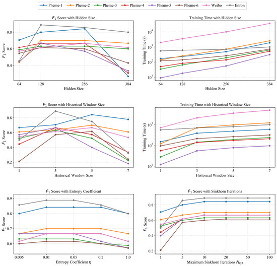
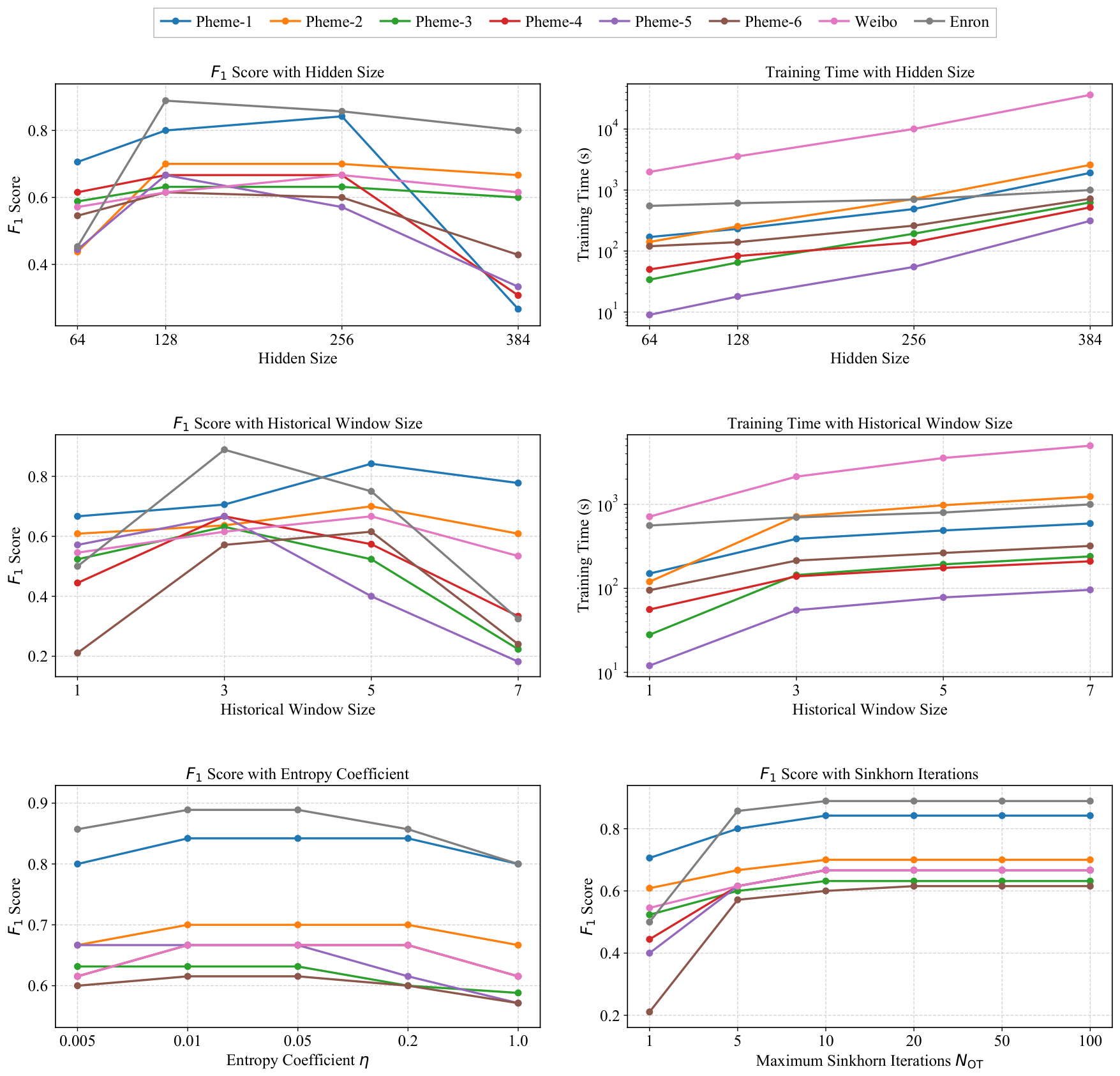
Figure 3 reports the sensitivity of ECPD-SG to hidden size, historical window size, and OT-related hyperparameters. For hidden size, most of the datasets reached peak or near-peak $F_1$ at $d=128$, with performance remaining competitive at $d=256$ but at notably higher training cost. Increasing d to 384 led to consistent $F_1$ degradation across most of the datasets, suggesting that excessively large representations are prone to overfitting on sparse social graphs. These results indicate that a moderate hidden size provides a favorable balance between model capacity and generalization. For historical window size, $F_1$ generally improved as the window increased from 1 to 3 or 5, suggesting that a short historical context helps stabilize representations and capture local evolution patterns. Extending the window to 7, however, led to degradation on most datasets, likely because longer aggregation windows dilute recent transition signals with earlier stable patterns. For the entropy coefficient $\eta$, performance was relatively stable around $\eta =0.01$ to $\eta =0.05$ across most of the datasets, and it remained competitive at $\eta =0.2$ on several of the datasets. When $\eta$ became too large, the transport plan tended to be over-smoothed, which weakened tee prototype-level correspondences and led to a drop in $F_1$ on most of the datasets. For the maximum Sinkhorn iterations $N_{\mathrm{OT}}$, $F_1$ improved noticeably from $N_{\mathrm{OT}}=1$ to 10 and then became stable in most cases, indicating that the OT alignment had largely converged after a moderate number of iterations. These results justify the default choices of $\eta =0.05$ and $N_{\mathrm{OT}}=100$.

Figure 3. Sensitivity of ECPD-SG to hidden size, historical window size, and OT-related hyperparameters across eight datasets. The first two rows report the effect of hidden size and historical window size in terms of $F_1$ and training time, while the last row reports the effect of the entropy coefficient $\eta$ and the maximum Sinkhorn iterations $N_{\mathrm{OT}}$ on $F_1$.

5.5. Case Study

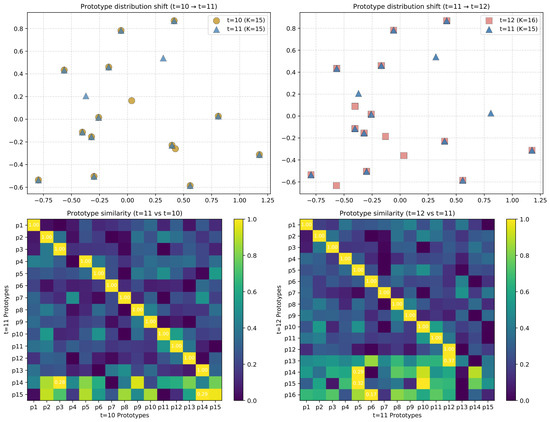
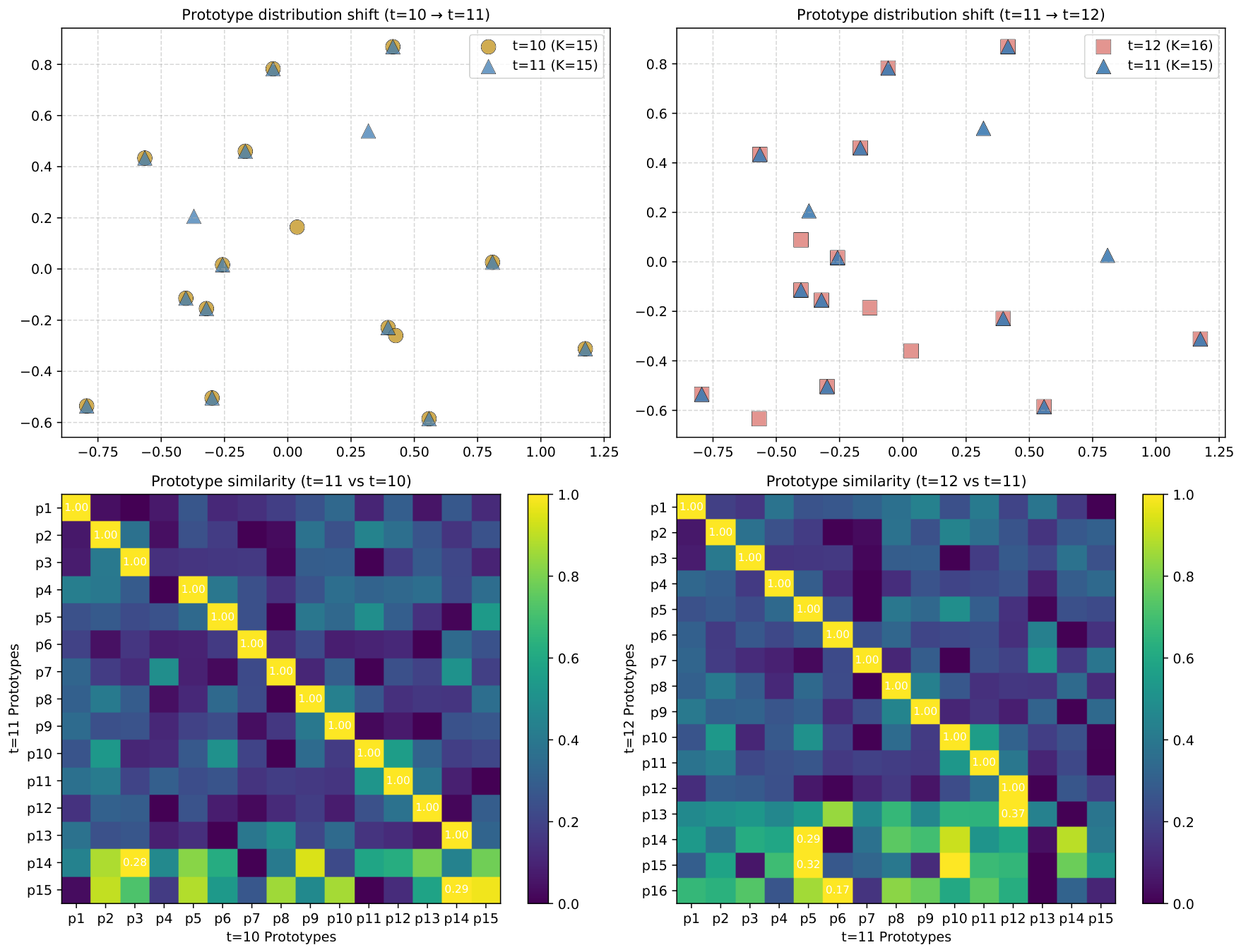
To further examine the interpretability of the prototype dynamics module, we analyzed the evolution of the prototype distributions across consecutive months on the Enron dataset, as shown in Figure 4. From October to November, the prototypes remained largely stable in the embedding space, and the similarity heatmap exhibited a clear diagonal pattern, indicating that the group-level interaction structure was consistent across this period, with most pf the prototypes maintaining strong cross-time alignment. From November to December, the prototype distributions showed more pronounced displacement, and the heatmap exhibited weaker diagonal similarity with stronger off-diagonal responses, suggesting that the prototype groups underwent reassignment or reorganization, reflecting a substantial shift in the underlying communication structure. These observations confirm that prototype shift patterns are interpretable indicators of structural transitions, consistent with the ground-truth change point occurring at this boundary.

Figure 4. Prototype evolution on the Enron dataset across two consecutive transitions: October to November ($t=10\to t=11$, left) and November to December ($t=11\to t=12$, right). The top row shows prototype distributions projected by t-SNE, and the bottom row shows pairwise cosine similarity matrices between prototypes from adjacent snapshots.

6. Conclusions

In this paper, we propose ECPD-SG, an emotion-aware contrastive prototype learning framework for change point detection in dynamic social graphs. ECPD-SG integrates textual semantics and emotional signals into temporal graph modeling and, furthermore, it summarizes evolving node representations into dynamic prototypes to capture group-level structural transitions. Our experiments on Pheme, Weibo, and Enron showed that ECPD-SG achieved competitive or superior performance over the representative baselines, while our ablation studies and case analysis verified the effectiveness and interpretability of emotion-aware modeling and prototype dynamics. In future work, we will extend ECPD-SG to larger-scale heterogeneous social graphs and develop online detection strategies for streaming scenarios.

References

- Mathioudakis, M.; Koudas, N. Twittermonitor: Trend detection over the twitter stream. In Proceedings of the ACM SIGMOD International Conference on Management of Data, SIGMOD, Indianapolis, IN, USA, 6–10 June 2010; Association for Computing Machinery: New York, NY, USA, 2010; pp. 1155–1158. [Google Scholar]
- Liu, C.; Tian, Y.; Shi, Y.; Huang, Z.; Shao, Y. An analysis of public topics and sentiments based on social media during the COVID-19 Omicron Variant outbreak in Shanghai 2022. Comput. Urban Sci. 2024, 4, 19. [Google Scholar] [CrossRef] [Scilit]
- Shu, K.; Sliva, A.; Wang, S.; Tang, J.; Liu, H. Fake news detection on social media: A data mining perspective. ACM SIGKDD Explor. Newsl. 2017, 19, 22–36. [Google Scholar]
- Huang, S.; Hitti, Y.; Rabusseau, G.; Rabbany, R. Laplacian Change Point Detection for Dynamic Graphs. In Proceedings of the ACM SIGKDD Conference on Knowledge Discovery and Data Mining, KDD, Virtual Event, 6–10 July 2020; Association for Computing Machinery: New York, NY, USA, 2020; pp. 349–358. [Google Scholar]
- Huang, S.; Coulombe, S.; Hitti, Y.; Rabbany, R.; Rabusseau, G. Laplacian Change Point Detection for Single and Multi-View Dynamic Graphs. ACM Trans. Knowl. Discov. Data 2024, 18, 1–32. [Google Scholar] [CrossRef] [Scilit]
- Zhu, T.; Li, P.; Yu, L.; Chen, K.; Chen, Y. Change Point Detection in Dynamic Networks Based on Community Identification. IEEE Trans. Netw. Sci. Eng. 2020, 7, 2067–2077. [Google Scholar] [CrossRef] [Scilit]
- Yu, W.; Cheng, W.; Aggarwal, C.C.; Zhang, K.; Chen, H.; Wang, W. NetWalk: A Flexible Deep Embedding Approach for Anomaly Detection in Dynamic Networks. In Proceedings of the ACM SIGKDD Conference on Knowledge Discovery and Data Mining, KDD, London, UK, 19–23 August, 2018; Association for Computing Machinery: New York, NY, USA, 2018; pp. 2672–2681. [Google Scholar]
- Sulem, D.; Kenlay, H.; Cucuringu, M.; Dong, X. Graph Similarity Learning for Change-Point Detection in Dynamic Networks. Mach. Learn. 2024, 113, 1–44. [Google Scholar]
- Kei, Y.L.; Li, J.; Li, H.; Chen, Y.; Madrid Padilla, O.H. Change Point Detection in Dynamic Graphs with Decoder-only Latent Space Model. Trans. Mach. Learn. Res. 2025. Available online: https://tmlr.infinite-conf.org/paper_pages/DVeFqV56Iz.html (accessed on 28 June 2026).
- Penaloza, E.; Stevens, N. Changepoint Detection in Highly-Attributed Dynamic Graphs. arXiv 2024, arXiv:2407.06998. [Google Scholar]
- Peel, L.; Clauset, A. Detecting Change Points in the Large-Scale Structure of Evolving Networks. In Proceedings of the AAAI Conference on Artificial Intelligence, AAAI, Austin, TX, USA, 25–30 January 2015; Association for the Advancement of Artificial Intelligence (AAAI): Washington, DC, USA, 2015; pp. 2914–2920. [Google Scholar]
- Wang, Y.; Chakrabarti, A.; Sivakoff, D.; Parthasarathy, S. Fast Change Point Detection on Dynamic Social Networks. In Proceedings of the International Joint Conference on Artificial Intelligence, IJCAI, Melbourne, Australia, 19–25 August 2017; AAAI Press: Washington, DC, USA, 2017; pp. 2992–2998. [Google Scholar]
- Awal, A.; Pandit, F. A Survey of Nature-Inspired Meta-Heuristic Algorithms in Network Alignment. Adv. Eng. Intell. Syst. 2024, 3, 15–38. [Google Scholar]
- Basiri, M.E.; Nemati, S.; Abdar, M.; Cambria, E.; Acharya, U.R. ABCDM: An Attention-Based Bidirectional CNN-RNN Deep Model for Sentiment Analysis. Future Gener. Comput. Syst. 2021, 115, 279–294. [Google Scholar]
- Horner, C.G.; Galletta, D.; Crawford, J.; Shirsat, A. Emotions: The unexplored fuel of fake news on social media. J. Manag. Inf. Syst. 2021, 38, 1039–1066. [Google Scholar] [CrossRef] [Scilit]
- Pho, K.H. Recommended System Optimization in Social Networks Based on Cooperative Filter with Deep MVR Algorithm. Adv. Eng. Intell. Syst. 2022, 1, 41–49. [Google Scholar]
- Lu, X. Detecting Depression via Tweets on Twitter Utilizing Machine Learning and Neural Network Models. J. Artif. Intell. Syst. Model. 2025, 3, 1–14. [Google Scholar]
- Khalid, M.; Sano, A. Exploiting Social Graph Networks for Emotion Prediction. Sci. Rep. 2023, 13, 6069. [Google Scholar] [CrossRef] [Scilit] [PubMed]
- Yan, J.; Pu, P.; Jiang, L. Emotion-RGC Net: A novel approach for emotion recognition in social media using RoBERTa and Graph Neural Networks. PLoS ONE 2025, 20, e0318524. [Google Scholar] [PubMed]
- Li, C.; Li, F. Emotion recognition of social media users based on deep learning. PeerJ Comput. Sci. 2023, 9, e1414. [Google Scholar] [CrossRef] [Scilit] [PubMed]
- Anoop, V.S.; Krishna, C.S.; Govindarajan, U.H. Graph embedding approaches for social media sentiment analysis with model explanation. Int. J. Inf. Manag. Data Insights 2024, 4, 100221. [Google Scholar] [CrossRef] [Scilit]
- Katalinić, J.; Dunđer, I. Neural Network-Based Sentiment Analysis and Anomaly Detection in Crisis-Related Tweets. Electronics 2025, 14, 2273. [Google Scholar]
- Chen, K.J.; Liu, L.; Jiang, L.; Chen, J. Self-supervised dynamic graph representation learning via temporal subgraph contrast. ACM Trans. Knowl. Discov. Data 2023, 18, 1–20. [Google Scholar] [CrossRef] [Scilit]
- Bao, P.; Li, J.; Yan, R.; Liu, Z. Dynamic graph contrastive learning via maximize temporal consistency. Pattern Recognit. 2024, 148, 110144. [Google Scholar]
- Chen, H.; Jiao, P.; Tang, H.; Wu, H. Temporal Graph Representation Learning with Adaptive Augmentation Contrastive. In Proceedings of the European Conference on Machine Learning and Principles and Practice of Knowledge Discovery in Databases, PAKDD, Turin, Italy, 18–22 September 2023; Springer Nature: Cham, Switzerland, 2023; pp. 683–699. [Google Scholar]
- Zhu, Z.; Wang, K.; Liu, H.; Li, J.; Luo, S. Topology-Monitorable Contrastive Learning on Dynamic Graphs. In Proceedings of the ACM SIGKDD Conference on Knowledge Discovery and Data Mining, KDD, Barcelona, Spain, 25–29 August 2024; Association for Computing Machinery: New York, NY, USA, 2024; pp. 4700–4711. [Google Scholar]
- Sankar, A.; Wu, Y.; Gou, L.; Zhang, W.; Yang, H. DySAT: Deep Neural Representation Learning on Dynamic Graphs via Self-Attention Networks. In Proceedings of the ACM International Conference on Web Search and Data Mining, WSDM, Houston, TX, USA, 3–7 February 2020; Association for Computing Machinery: New York, NY, USA, 2020; pp. 519–527. [Google Scholar]
- Page, E.S. Continuous inspection schemes. Biometrika 1954, 41, 100–115. [Google Scholar] [CrossRef] [Scilit]
- Zubiaga, A.; Liakata, M.; Procter, R. Exploiting Context for Rumour Detection in Social Media. In Proceedings of the International Conference on Social Informatics, Oxford, UK, 13–15 September 2017; Springer: Cham, Switzerland, 2017; pp. 109–123. Available online: https://figshare.com/articles/dataset/PHEME_dataset_for_Rumour_Detection_and_Veracity_Classification/6392078 (accessed on 24 June 2026).
- Ma, J.; Gao, W.; Mitra, P.; Kwon, S.; Jansen, B.J.; Wong, K.F.; Cha, M. Detecting Rumors from Microblogs with Recurrent Neural Networks. In Proceedings of the International Joint Conference on Artificial Intelligence, IJCAI, New York, NY, USA, 9–15 July 2016; AAAI Press: Washington, DC, USA, 2016; pp. 3818–3824. Available online: https://www.dropbox.com/s/46r50ctrfa0ur1o/rumdect.zip?dl=0 (accessed on 24 June 2026).
- Klimt, B.; Yang, Y. Introducing the Enron Corpus. In Proceedings of the Conference on Email and Anti-Spam, CEAS, Mountain View, CA, USA, 30–31 July 2004; pp. 92–96. Available online: https://www.cs.cmu.edu/~enron/ (accessed on 24 June 2026).
- Paszke, A.; Gross, S.; Massa, F.; Lerer, A.; Bradbury, J.; Chanan, G.; Killeen, T.; Gimelshein, N.; Antiga, L.; Desmaison, A.; et al. PyTorch: An Imperative Style, High-Performance Deep Learning Library. In Proceedings of the Annual Conference on Neural Information Processing Systems, NeurIPS, Vancouver, BC, Canada, 8–14 December 2019; Curran Associates Inc.: Red Hook, NY, USA, 2019; pp. 8024–8035. [Google Scholar]
- Reimers, N.; Gurevych, I. Sentence-BERT: Sentence Embeddings using Siamese BERT-Networks. In Proceedings of the Conference on Empirical Methods in Natural Language Processing, EMNLP, Hong Kong, China, 3–7 November 2019; Association for Computational Linguistics: Stroudsburg, PA, USA, 2019; pp. 3980–3990. [Google Scholar]
- Mohammad, S.M.; Turney, P.D. Crowdsourcing a Word–Emotion Association Lexicon. Comput. Intell. 2017, 29, 436–465. [Google Scholar]
- Bird, S.; Klein, E.; Loper, E. Natural Language Processing with Python: Analyzing Text with the Natural Language Toolkit; O’Reilly Media, Inc.: Sebastopol, CA, USA, 2009. [Google Scholar]
- Xu, L.; Lin, H.; Pan, Y.; Ren, H.; Chen, J. Constructing the Affective Lexicon Ontology. J. China Soc. Sci. Tech. Inf. 2008, 27, 180–185. [Google Scholar]
- Dong, Z.; Dong, Q. HowNet: A Hybrid Language and Knowledge Resource. In Proceedings of the International Conference on Natural Language Processing and Knowledge Engineering, NLPKE; IEEE: Piscataway, NJ, USA, 2003; pp. 820–824. [Google Scholar]
Disclaimer/Publisher’s Note: The statements, opinions and data contained in all publications are solely those of the individual author(s) and contributor(s) and not of MDPI and/or the editor(s). MDPI and/or the editor(s) disclaim responsibility for any injury to people or property resulting from any ideas, methods, instructions or products referred to in the content. |
© 2026 by the authors. Licensee MDPI, Basel, Switzerland. This article is an open access article distributed under the terms and conditions of the Creative Commons Attribution (CC BY) license.