


Abstract
Rotating machinery is a key component in modern industry, and its operating condition directly affects equipment safety and production reliability. However, discrepancies among different machines cause source–target distribution shifts, while fault annotation for target machines is costly, limiting the performance of deep learning-based diagnosis under cross-machine scenarios with limited labels. To address these issues, this paper proposes a multi-scale time–frequency semantic consistency model based on self-supervised transferable representation learning, termed MTFSC. First, augmented waveform views and multi-scale frequency-domain views are constructed from unlabeled source-domain vibration signals for self-supervised pre-training without source labels. Then, a time-domain impulse-aware feature extractor and a time–frequency decoupled spectral feature extractor are designed to enhance local impulsive responses and emphasize fault-sensitive time–frequency patterns. Furthermore, a semantic-aware soft contrastive loss is developed to mine potential semantic neighbors from multi-scale frequency-domain structural similarity, reducing false-negative effects in conventional hard-label contrastive learning. Finally, the pre-trained time-domain extractor is transferred to the target machine and fine-tuned with limited labeled samples. Experimental results show that MTFSC outperforms comparison methods under different labeled sample ratios and achieves an average accuracy of 97.5% across four cross-machine diagnostic tasks.
1. Introduction
Rotating machinery constitutes a critical power transmission and supporting unit for the long-term stable operation of mechanical equipment, and is widely used in rail transportation, aerospace, and industrial production systems. During long-term service, such machinery is commonly subjected to alternating loads, impulsive vibrations, and complex environmental disturbances. Once faults occur, they may lead to equipment shutdown or even serious safety accidents [1,2]. Therefore, timely and accurate identification of the operating condition of rotating machinery and determination of fault types are of great significance for ensuring equipment safety, reducing maintenance costs, and improving the reliability of industrial systems [3,4].
Traditional fault diagnosis (FD) methods for rotating machinery generally extract fault features through time–frequency analysis and signal decomposition techniques, followed by machine learning-based classifiers for condition identification [5,6,7]. However, these methods usually rely on expert experience for feature design and exhibit limited adaptability to different working scenarios and non-stationary operating conditions. When equipment structures and operating conditions vary, the stability and generalization capability of handcrafted features are often difficult to guarantee. With the development of sensing technologies, the Industrial Internet of Things, and big data analytics, deep learning-based intelligent FD has gradually become an important research direction in the field of rotating machinery health monitoring. Since deep learning models can automatically mine deep nonlinear features from input signals, they demonstrate strong feature representation capability in complex fault identification tasks. Hou et al. [8] fed frequency–domain features extracted by FFT into an improved Transformer architecture, and extracted both local and global features through a multi-feature parallel fusion encoder and a cross-flipping decoder, achieving high recognition accuracy for rolling bearing faults. Yuan et al. [9] employed SE-Conv1d to adaptively enhance key features and modeled long-sequence global dependencies using a ProbSparse self-attention mechanism, thereby improving the accuracy and stability of bearing FD. Zou et al. [10] developed a three-channel FD model integrating a convolutional autoencoder, multimodal time–frequency representations, and a dual-attention mechanism, enabling deep multi-domain feature mining and high-accuracy classification under strong noise conditions. He et al. [11] proposed an adaptive graph framework convolutional network, in which vibration signals were constructed as graph structures and dynamic graph learning and framelet transform convolution were introduced to enhance fault feature extraction under complex operating conditions. These studies demonstrate that deep learning methods can effectively improve the performance of rotating machinery FD, particularly showing clear advantages in nonlinear feature extraction and fault identification under complex working conditions.
Although deep learning methods have made significant progress in rotating machinery FD, several key limitations remain in practical engineering applications. First, most deep learning-based diagnostic models rely on large amounts of high-quality labeled data for training. However, rotating machinery typically operates in a healthy state for long periods, resulting in a limited number of real fault samples. Moreover, fault data annotation usually requires domain expertise and experimental verification, making it costly to obtain reliable labels [12,13]. In addition, most supervised learning models assume that the training and testing data follow identical or similar distributions. In real industrial scenarios, however, variations may exist in equipment types, mechanical structures, transmission paths, rotational speeds, and sampling conditions, leading to significant distribution discrepancies between the source and target domains [14,15]. For different machines or operating conditions, data often need to be recollected, samples relabeled, and diagnostic models retrained, which not only increases the cost of model deployment but also restricts the widespread application of deep learning methods across multiple devices and scenarios. Therefore, how to fully exploit existing data to learn transferable and generalizable fault representations under limited labeled samples from the target machine has become an important issue in intelligent FD of rotating machinery.
To mitigate the effects of data distribution discrepancies and insufficient target-domain annotations, transfer learning and cross-domain diagnostic methods have been widely introduced into rotating machinery FD. Huang et al. [16] proposed a deep multi-source transfer learning model, which selects appropriate source-domain data using maximum mean discrepancy and improves multi-source cross-condition transfer diagnosis performance by combining independent domain-specific feature extractors, Wasserstein distance, and a weighted decision mechanism. Li et al. [17] integrated multi-kernel MMD and conditional MMD into a joint distribution metric, and enhanced cross-condition diagnostic capability through adaptive weighting and pseudo-label correction mechanisms. Considering the class imbalance phenomenon in practical industrial monitoring, where normal samples are far more abundant than fault samples, Luo et al. [18] proposed a dynamic maximum three-view classifier discrepancy network to improve imbalanced cross-domain FD performance. The above methods improve cross-domain diagnostic performance from the perspectives of distribution alignment, adversarial learning, and pseudo-label optimization. However, most existing studies mainly focus on transfer problems across different operating conditions of the same machine. When the diagnostic object is extended to different machines, the discrepancies in mechanical structures, fault modes, and signal transmission paths become more pronounced. In such cases, cross-domain methods that rely solely on distribution alignment or pseudo-label optimization are prone to feature mismatching, negative transfer, and insufficient generalization. Compared with cross-condition diagnosis, cross-machine FD is more consistent with practical engineering deployment scenarios and is also more challenging. Under cross-machine conditions, the source and target machines may differ in bearing types, structural parameters, operating ranges, and fault generation mechanisms, resulting in substantially enlarged discrepancies in fault signal distributions [19,20]. Zhao et al. [21] addressed the problems of large domain discrepancies and low recognition accuracy in cross-machine bearing FD by proposing a cross-domain adaptive clustering and dynamic thresholding method. This method generates pseudo-labels through adversarial clustering loss and class-specific dynamic thresholds, thereby improving the stability of clustering cores under few-shot target-domain conditions. From the perspective of causal representation learning, Jia et al. [22] proposed a deep causal disentanglement network, in which cross-machine generalizable fault representations are regarded as causal factors, while machine-related representations are treated as non-causal factors. Stable fault representations are learned through causal task decomposition and feature disentanglement. Guo et al. [23] employed a structural causal model to decompose multi-source-domain fault data into fault-related causal factors and domain-related non-causal factors, and enhanced cross-machine generalization capability through causal aggregation, entropy maximization, contrastive estimation, and redundancy reduction losses. These studies have effectively advanced the development of cross-machine FD. Nevertheless, several limitations remain. Most cross-machine diagnostic methods still rely on labeled source-domain data or multi-source-domain annotation information to learn discriminative decision boundaries. In addition, complex procedures such as causal disentanglement, domain alignment, or pseudo-label filtering may increase the training complexity of the model. Moreover, when only very few labeled samples are available in the target domain, or when substantial discrepancies exist between the target and source machines, the stability of the learned feature representations still requires further improvement.
Self-supervised pre-training knowledge transfer (SSPKT) provides a new perspective for addressing the aforementioned issues. Its basic idea is to pre-train a feature extractor in a data-rich source domain, enabling the model to learn general fault representations, and then transfer it to downstream diagnostic tasks in the target domain for fine-tuning with only a small number of labeled samples [24,25]. Compared with direct supervised training, SSPKT can mine latent structural information from unlabeled data through predefined pretext tasks, allowing the model to learn useful representations without relying on manual annotations. In recent years, SSPKT has been introduced into rotating machinery FD [26,27]. Xu et al. [28] constructed time-domain augmentations, frequency-domain prediction, and a cross-correlation smoothed matrix loss function to learn effective representations from unlabeled traction motor bearing fault data, achieving efficient train bearing FD with only a few labeled samples. Fan et al. [29] proposed a time–frequency residual self-supervised (SS) network based on an improved MoBY framework, where time–frequency representations were used to construct a contrastive pre-training task, and a dynamic queue and fault-signal augmentation strategy were incorporated to enhance feature extraction performance under limited-label conditions. He et al. [30] designed a dual-encoder and a time–frequency fusion encoder, and jointly optimized the model using time–frequency contrastive loss and time–frequency fusion loss, enabling it to learn latent fault representations from unlabeled time–frequency signals. These SS methods effectively reduce the dependence of diagnostic models on labeled data. However, they mainly focus on few-shot diagnosis within the same dataset or the same platform, and their adaptability to cross-machine distribution discrepancies remains limited. Some contrastive learning methods rely on the construction of positive and negative sample pairs, which may incorrectly treat different samples with similar fault patterns as negative samples. Therefore, a few researchers have begun to explore SS pre-training diagnostic methods for cross-machine scenarios. Chen et al. [31] exploited the consistency between waveform and spectrogram representations to learn transferable features from unlabeled source-domain fault data, and transferred the pre-trained encoder to multiple cross-machine downstream diagnostic tasks. Zhao et al. [32] proposed a multi-task SS transfer learning framework, in which mask tasks at different scales were used to enhance the model’s attention to the intrinsic structure of bearing vibration signals, while probability distribution and geometric similarity metrics were combined to achieve multi-view feature transfer. Wang et al. [33] proposed an SS-enhanced open-set cross-machine diagnostic method, integrating open-set risk minimization, SS contrastive learning, and pseudo-label consistency self-training to improve unknown fault recognition and cross-machine transfer performance. These studies indicate that SS pre-training has great potential in cross-machine FD. Although cross-machine SS pre-training methods provide an effective solution for FD of target machines with limited annotations, they still face several challenges in complex engineering scenarios. Cross-machine diagnosis involves multi-factor discrepancies, and source-domain pre-trained representations are prone to insufficient transfer or even performance degradation in the target domain. In addition, most existing SS pretext tasks construct training objectives from the perspectives of view consistency, instance discrimination, or masked reconstruction, while insufficient consideration is given to the inherent time-varying impulses, frequency-band responses, and latent semantic relationships among samples in fault signals. Consequently, the discriminability and robustness of the pre-trained features are still limited under complex noise interference and cross-domain distribution shifts.
To address the aforementioned issues, this paper proposes a multi-scale time–frequency semantic consistency (MTFSC) model based on SS transferable representation learning. This method constructs enhanced waveform views and multi-scale frequency-domain views from the unannotated vibration signals of the source domain, and learns transferable fault representations through dual-branch SS pre-training. At the feature extraction level, a time-domain pulse-aware feature extractor and a frequency-domain time–frequency decoupling feature extractor are designed, enabling the model to focus on local pulse segments in the waveform, key time frames in the frequency-domain view, and frequency bands sensitive to faults. In the pre-training objective, a semantic-aware soft contrastive loss is constructed, based on the structural similarity of multi-scale frequency-domain representations, to assign soft positive weights to potential semantic neighborhoods, thereby alleviating the false negative problem in traditional contrastive learning. After pre-training, the time-domain encoder is retained as the backbone for downstream diagnosis and is fine-tuned using a small number of labeled samples from the target machine to achieve cross-machine fault identification. It is important to note that MTFSC does not simply combine waveform enhancement, time–frequency representation, attention modules, and contrastive learning. Instead, these components are designed based on the inherent characteristics of rotating machinery fault signals and the requirements of cross-machine transferable representation learning. Specifically, waveform signals are more sensitive to local impacts and periodic transient responses, while multi-scale frequency-domain views can provide complementary descriptions of fault-sensitive frequency-band structures at different time–frequency resolutions. Therefore, the dual-branch architecture is designed to extract complementary fault information from these two views. Additionally, different samples with similar fault mechanisms may exhibit similar time–frequency structures. If the traditional hard-label contrastive learning method is directly adopted, these semantically similar samples may be wrongly regarded as negative samples and pulled apart in the representation space. To solve this problem, the proposed semantic-aware soft contrastive loss utilizes the structural similarity of multi-scale frequency domain views to explore potential semantic neighborhoods, thereby enhancing the organization and transferability of the self-supervised feature space. This framework achieves a unified design in signal representation, feature extraction, and learning objectives, rather than simply stacking existing modules. The main contributions of this paper are summarized as follows:
The main contributions of this paper are summarized as follows:
- (1)
- An SS transferable representation learning framework is proposed for cross-machine FD of rotating machinery. The framework can perform pre-training using unlabeled source-domain signals without relying on source-domain fault labels to train a fixed classifier. By learning the consistency between waveform and frequency-domain representations, it obtains general fault representations suitable for few-shot diagnosis on target machines.
- (2)
- A fault-sensitive dual-branch feature extraction structure is constructed. For local impulsive characteristics in waveform signals, a time-domain impulse attention module is designed to enhance critical transient responses. Meanwhile, a time–frequency decoupled attention module is developed to emphasize key time frames and fault-sensitive frequency bands, thereby improving the discriminability and stability of fault features under cross-machine conditions.
- (3)
- A semantic-aware soft contrastive loss function is designed. This loss mines potential semantic neighbors by measuring the similarity among multi-scale frequency-domain views. While maintaining strong cross-view consistency for the same sample, it avoids excessively separating similar fault segments, thereby improving the semantic organization of the SS feature space and enhancing the transfer diagnostic performance of the model under limited labeled samples from the target machine.
The remainder of this paper is organized as follows. Section 2 introduces the overall framework of the proposed method, including dual-view construction, feature extractors, and the semantic-aware soft contrastive loss function. Section 3 describes the experimental datasets, preprocessing procedures, comparison methods, and experimental settings. Section 4 presents the ablation studies and cross-machine diagnostic results. Finally, Section 5 concludes this paper and discusses future research directions.
2. Methodology
2.1. The Basic Framework and Workflow of MTFSC
To address the issues of insufficient labeled samples in the target domain and the susceptibility of fault features to variations in operating conditions in cross-machine FD of rotating machinery, this paper develops an MTFSC model based on SS transferable representation learning. MTFSC constructs waveform views and multi-scale frequency-domain views from unlabeled fault signals in the source domain, and learns consistent representations of the two types of views in the latent space through a dual-branch encoder. In this way, the model can be pre-trained without relying on source-domain labels to train a fixed category classifier. Subsequently, the pre-trained time-domain encoder is transferred to the target-domain diagnostic task, and the classifier is fine-tuned using a small number of labeled target samples.
Let the unlabeled data set of the source domain be represented as , where Ns denotes the number of source-domain samples, and is a one-dimensional vibration signal segment of length N. Similarly, let the small-labeled data set of the target domain be represented as , where Nt denotes the number of target-domain samples, is the target fault category label. The workflow of MTFSC is mainly shown in Figure 1, which mainly consists of three stages:
Figure 1.
MTFSC FD workflow diagram.
Stage 1: First, the unlabeled vibration signals in the source domain are normalized and segmented to obtain signal samples with a unified length. Then, two complementary views are constructed from the same signal. An augmented waveform view is generated through random noise perturbation to preserve time-domain information such as fault impulses, abrupt amplitude variations, and periodic fluctuations. In addition, multi-scale frequency-domain views are generated using multiple short-time Fourier transform (STFT) window lengths to characterize the energy distributions under different time-frequency resolutions. Through this dual-view construction strategy, the model can simultaneously obtain the temporal dynamic characteristics and frequency-domain structural characteristics of fault signals, thereby providing the input basis for subsequent SS consistency learning.
Stage 2: In the pre-training stage, the two complementary views are fed into the time-domain impulse perception feature extractor (TIPFE) and the frequency-domain time–frequency decoupling feature extractor (FTDFE), respectively. The time-domain branch is used to extract local impulsive and periodic modulation information from waveforms, while the frequency-domain branch is used to capture key time frames and fault-sensitive frequency bands from spectrograms. Subsequently, the two types of features are mapped into a unified latent representation space through dual projection heads and constrained by the semantic-aware soft contrastive loss. This loss not only enforces consistency between the waveform and frequency-domain features of the same sample, but also mines potential semantic neighbors by exploiting multi-scale frequency-domain similarity, thereby alleviating the problem that similar fault samples may be incorrectly treated as negative samples in conventional contrastive learning. Through this stage, the model can learn fault-sensitive and cross-domain transferable representations from abundant unlabeled source-domain data.
Stage 3: After self-supervised pre-training, the frequency-domain branch and the projection heads are removed, and the pre-trained TIPFE is retained as the backbone of the target-domain diagnostic model. A new fully connected classification layer is then initialized according to the number of fault categories in the target domain. During fine-tuning, the labeled target-domain samples are input into the TIPFE to obtain fault feature representations, and the classification layer outputs the predicted category probabilities. The downstream model is optimized using the cross-entropy loss calculated between the predicted labels and the true labels. Finally, the fine-tuned model is used to predict the fault categories of the target-domain test samples.
2.2. Wave Enhancement and Construction of Multi-Scale Frequency-Domain Views
Fault signals of rotating machinery usually contain information such as local impulses, periodic modulation, background noise, and variations in frequency-band energy. A single time-domain or frequency-domain representation is insufficient to comprehensively characterize the feature differences among different fault modes. Therefore, in this paper, two complementary views are constructed based on the same raw signal. Specifically, the waveform view is formed by adding random perturbations to the raw signal, so as to preserve the impulsive and fluctuating information in the original time series. In addition, a multi-scale frequency-domain view is constructed using multiple STFT scales to describe the energy distribution under different time-frequency resolutions. These two views jointly provide cross-view consistency constraints for SS pre-training. Figure 2 shows a set of signals that have undergone wavelet enhancement and multi-scale STFT transformation from the original signals.
Figure 2.
Example of wave enhancement samples and construction of multi-scale frequency-domain view.
2.2.1. Wave Enhancement
In SS pre-training, the role of data augmentation is not to alter the semantic information of fault categories, but to provide reasonable perturbations that enable the model to learn features more robust to noise and variations in operating environments. Considering that vibration signals collected in industrial fields are often affected by sensor noise, background vibration, electromagnetic interference, and other factors, random signal-to-noise ratio Gaussian noise is adopted to construct the augmented waveform view. For the i-th source-domain signal xi, its augmented waveform can be expressed as
where denotes the augmented waveform view, represents the added Gaussian noise, N is the signal length, denotes the L2-norm of the signal, SNRi is the signal-to-noise ratio randomly sampled from the predefined range, and SNRmin and SNRmax are the lower and upper bounds of the SNR range, respectively. Through this augmentation strategy, the model is exposed to signal patterns under different noise levels during the pre-training stage, thereby improving the adaptability of the time-domain encoder to field noise and cross-condition disturbances.
2.2.2. Construction of Multi-Scale Frequency-Domain View
The frequency-domain view is used to characterize the energy distribution of fault signals in the time–frequency plane. Conventional single-scale STFT usually requires a trade-off between time resolution and frequency resolution. A shorter window is beneficial for capturing transient impulses, but provides insufficient frequency resolution. In contrast, a longer window can provide a clearer frequency structure, but may weaken the temporal localization capability for local impulses. To fully preserve fault information at different scales, this paper applies STFT to the same signal using multiple window lengths, and the resulting spectrograms are resized to a unified scale and concatenated to form a multi-channel frequency-domain view.
Let Lm denote the window length of the m-th STFT scale, Hm denote the hop size, and wm(n) denote the window function. Then, the frequency-domain representation of the i-th signal at this scale can be written as
where denotes the spectral energy at the q-th time frame and the p-th frequency bin under the m-th scale, Lm is the Fourier window length, Hm is the hop size, and wm(n) is the window function. To reduce the influence of extreme amplitude variations in the spectrogram on model training, the spectrogram is further processed by logarithmic compression and normalization:
Subsequently, the spectrograms at different scales were resampled to a uniform size and concatenated along the channel dimension to obtain a multi-scale frequency-domain view:
where M denotes the number of STFT scales, and H and W denote the unified frequency dimension and time-frame dimension, respectively. In the implementation of this paper, multiple STFT window lengths are adopted to construct the multi-channel frequency-domain input. A shorter window mainly captures transient impact-related energy changes, a longer window emphasizes stable frequency components and harmonic structures, and a medium window balances these two aspects to reflect repeated impact and modulation patterns. Therefore, the multi-scale spectrogram input provides complementary time–frequency information for the frequency-domain encoder.
2.3. SS Pre-Training Process
The objective of the SS pre-training stage is to learn fault representations with cross-machine transferability without using source-domain class labels. For the same signal xi, although the augmented waveform view and the multi-scale frequency-domain view originate from different representation domains, they reflect the fault information under the same mechanical state. Therefore, the two views should exhibit high consistency in the latent space. Based on this, this paper constructs an SS pre-training structure composed of a time-domain branch, a frequency-domain branch, and dual projection heads.
Given a set of pre-trained samples, the process of extracting their dual-view features can be expressed as
where Ft(·) denotes the time-domain impulse-aware feature extractor, Ff(·) denotes the frequency-domain time–frequency decoupled feature extractor, and are the learnable parameters of the two encoders, respectively, and ui and vi denote the time-domain feature and frequency-domain feature, respectively.
2.3.1. TIPFE
Time-domain waveforms contain information such as the temporal locations of fault impacts, abrupt amplitude variations, and periodic fluctuations. For rotating components such as bearings, damages on the outer race, inner race, and rolling elements are often manifested as local impacts and repetitive impulses, while these key features occupy only partial time intervals in the overall waveform. To make the model pay more attention to the transient responses related to faults, this paper introduces a time-domain impulse attention module after the high-level features of the one-dimensional residual network, forming a TIPFE, whose structure is shown in Figure 3.
Figure 3.
TIPFE structure diagram.
Let the output feature of the one-dimensional residual backbone at a certain stage be where C denotes the number of channels and L denotes the length of the temporal dimension. First, the average response and maximum response are calculated along the channel dimension, and the two responses are concatenated to form a temporal descriptor:
Subsequently, time attention weights are generated through one-dimensional convolution and the Sigmoid function:
where denotes the importance weights at different temporal positions, and is the Sigmoid activation function. Specifically, is calculated from the concatenated average-pooled and max-pooled temporal descriptor through a learnable one-dimensional convolution layer, and each value is normalized to the range of 0–1 by the Sigmoid function. Therefore, a larger value in indicates that the corresponding temporal position is more likely to contain fault-related impulsive information. To prevent the attention mechanism from excessively suppressing the original features at the early stage of training, a residual enhancement strategy is adopted in this paper to recalibrate the features:
In the formula, represents element-wise multiplication. Through this mechanism, the model can enhance the local impact segments while retaining the original time-domain representation, making the subsequent features more sensitive to the transient changes in the fault. Eventually, the enhanced high-level time-domain features are processed by subsequent residual blocks and global average pooling to obtain the time-domain representation ui.
2.3.2. FTDFE
The multi-scale frequency-domain view is essentially a two-dimensional time-frequency representation with explicit physical meanings, where the frequency axis reflects fault-sensitive frequency bands and harmonic structures, while the time axis indicates the occurrence locations and duration of impulsive responses. If it is directly treated as a conventional image and fed into a two-dimensional convolutional network, the differences between the temporal and frequency directions may be ignored. Therefore, this paper introduces a time–frequency decoupled attention module into the two-dimensional residual network, enabling the frequency-domain branch to separately focus on key time frames and important frequency bands. The structure of FTDFE is shown in Figure 4; the time–frequency decoupled attention module contains two parallel branches. For the input feature map , the frequency attention branch first aggregates the feature responses along the temporal dimension and then uses convolutional mapping and Sigmoid activation to generate the frequency attention map . Similarly, the temporal attention branch aggregates the feature responses along the frequency dimension and generates the temporal attention map . The two attention maps are broadcast to the same size as the input feature map and are used to recalibrate the original features through residual enhancement.
Figure 4.
FTDFE structure diagram.
Let the intermediate feature output by the two-dimensional residual backbone be where H denotes the frequency dimension and W denotes the temporal dimension. The frequency attention branch aggregates feature responses along the temporal dimension to describe the importance of different frequency bands, while the temporal attention branch aggregates feature responses along the frequency dimension to describe the importance of different time frames:
where denotes the frequency attention map, denotes the temporal attention map, and gf(·) and gt(·) represent the pooling and convolutional mapping operations in the frequency and temporal branches, respectively. Finally, the frequency-domain features are recalibrated using a residual enhancement strategy:
This structure can simultaneously enhance fault-sensitive frequency bands and transient impact time frames, enabling the frequency-domain features to no longer rely solely on local two-dimensional textures, but to further incorporate the physical meanings of the axes in the spectrogram. The enhanced frequency-domain features are then passed through subsequent convolutional layers and global pooling to obtain the frequency-domain representation vi.
Both of the above two feature extractors are adapted based on the residual bottleneck structure. Table 1 summarizes the detailed architectures of the two feature extractors. The trainable parameters of TIPFE and FTDFE are 6,312,398 and 13,866,204 respectively. The complete self-supervised pre-training network, including TIPFE, FTDFE and two projection heads, contains a total of 28,072,107 trainable parameters. These parameters are optimized using 4420 unlabeled training samples from the PU source-domain dataset. After pre-training, only TIPFE is retained for downstream diagnosis, and a new fully connected classification layer is initialized based on the health status of the eight target-domains. The downstream diagnostic model contains 6,316,502 trainable parameters, including 6,312,398 parameters from TIPFE and 4104 parameters from the classification layer. During downstream fine-tuning, the model is optimized using 32 labeled training samples from each target domain dataset. Validation and test samples are not used for parameter optimization.
Table 1.
Detailed information about the TIPFE and FTDFE feature extraction architectures.
2.3.3. Dual Projection Head Based on Self-Attention
The features output by TIPFE and FTDFE exhibit different statistical characteristics and representation emphases. To compare the consistency between the two types of features in a unified latent space, this paper assigns a projection head to each branch, mapping the high-dimensional features extracted by the feature extractors into low-dimensional representations suitable for SS alignment. Let Pt(·) and Pf(·) denote the time-domain projection head and the frequency-domain projection head, respectively. Then, this process can be expressed as
where hi and zi denote the representations of the time-domain view and the frequency-domain view in the consistency learning space, respectively. The projection head adopts a self-attention structure to model the relationships among feature dimensions. For the input feature ri, its query, key, and value vectors can be expressed as
The self-attention mapping process can be expressed as
Here, WQ, WK, and WV are learnable mapping matrices, and d denotes the feature dimension. Through the self-attention projection head, the model can adaptively reweight important components in the feature dimensions, enabling the time-domain and frequency-domain representations to exhibit more stable comparability in the unified representation space.
2.4. Semantic Perception Soft Contrastive Loss Function
In conventional cross-view contrastive learning, only two views of the same sample in a batch are usually regarded as a positive pair, while all other non-corresponding samples are treated as negative samples. However, in fault signals of rotating machinery, different samples may originate from similar fault patterns or exhibit similar frequency-band structures. If all these potentially similar samples are forcibly pushed apart, the false negative problem may arise, which can impair the intra-class compactness of the feature space. Therefore, this paper proposes the semantic-aware soft contrastive loss function as shown in Figure 5. A soft-label matrix is constructed based on the similarity between multi-scale frequency-domain views. While maintaining the strong consistency across views for the same sample, smaller positive weights are assigned to potential semantic neighbors.
Figure 5.
Principle diagram of semantic-aware soft contrastive loss function.
First, the projected time-domain representation hi and frequency-domain representation zj are normalized, and the cross-view similarity matrix is calculated as follows:
where sij denotes the similarity between the i-th time-domain feature and the j-th frequency-domain feature, and is a learnable temperature parameter. After Softmax normalization, the matching probability from the time domain to the frequency domain is obtained as
To mine potential semantic neighbors, this paper constructs semantic similarities among samples using the multi-scale frequency-domain views. Let denote the low-dimensional descriptor obtained from the multi-scale frequency-domain view. Then, the semantic similarity between samples is defined as
For each sample i, the top K similar samples are selected according to rij to form the semantic-neighbor set . At the early stage of training, a conventional hard-label contrastive loss is first adopted for warm-up to ensure stable convergence. After the warm-up stage, the soft-label matrix is constructed as follows:
Here, denotes the total soft positive weight assigned to semantic neighbors, is the temperature parameter for semantic-neighbor weight allocation, and represents the frequency-domain semantic-neighbor set of the i-th sample. When a sample has no neighbors satisfying the similarity threshold, its label degenerates into a one-hot form to avoid introducing unreliable soft positive samples.
Based on the soft-label matrix, the loss from the time domain to the frequency domain is defined as
Similarly, the loss from the frequency domain to the time domain, , can be obtained. The final SS pre-training loss is defined as
While optimizing the consistency between the two views of the same sample, this loss function exploits the multi-scale frequency-domain structure to mine potentially similar samples, allowing similar fault segments to remain moderately close in the feature space. In this way, the semantic organization capability of the SS representations and the robustness of cross-machine transfer are improved. After pre-training, the time-domain impulse-aware feature extractor is retained as the backbone for downstream diagnosis, and a classification head is trained using a small number of labeled samples from the target domain to achieve cross-machine fault identification.
3. Data Set and Experimental Design
3.1. Source and Introduction of the Experimental Data Set
3.1.1. Paderborn University Laboratory Equipment and Data
As shown in Figure 6, the Paderborn University (PU) bearing test rig [34] was constructed by Paderborn University in Germany and is mainly used for condition monitoring of external rolling bearings in electric motor drive systems. The tested bearing is installed in the rolling bearing test module, where different rotational speeds, load torques, and radial loads can be applied during the experiments. Vibration signals from the bearing housing were collected at a sampling frequency of 64 kHz. The PU dataset includes four typical operating conditions, corresponding to different combinations of rotational speed, load torque, and radial load.
Figure 6.
PU experimental platform and its components.
In this paper, the PU dataset is used only as the source-domain dataset for self-supervised pre-training. It contains 13 bearing health states, including one healthy state and 12 real damage states. The damage states mainly involve outer race faults, inner race faults, and compound inner-outer race faults with different damage forms, such as pitting and indentation. It should be emphasized that the health-state labels of the PU dataset are not used to train a supervised source-domain classifier. During the pre-training stage, the PU dataset is treated as unlabeled source-domain data, and MTFSC learns transferable fault representations through consistency learning between waveform views and multi-scale frequency-domain views.
3.1.2. Self-Built Bearing Fault Simulation Experimental Platform 1
To verify the cross-machine FD capability of the proposed MTFSC model under limited labeled samples from the target machine, an in-house bearing fault test rig was used to collect downstream target-domain data. As shown in Figure 7, the test platform mainly consists of a drive motor, tested bearing, brake, vibration sensor, and signal acquisition instrument. During the experiment, tested bearings with different fault types were sequentially mounted on the test rig, and the operating state of the bearing was adjusted using the control system. When the rotational speeds were stabilized at 1500 r/min and 2100 r/min, vibration response signals during bearing operation were collected using the vibration sensor. The sampling frequency was set to 20 kHz, and the continuous sampling duration for each health state was 60 s. The data collected under the two rotational speed conditions were used to construct target-domain diagnostic tasks, so as to evaluate the transfer adaptability of the model under different machines and operating conditions.
Figure 7.
Self-built experimental bench 1 and its components.
In the experiment, local cracks were machined at different bearing components using wire electrical discharge machining to simulate typical bearing damages that may occur during actual operation. The crack width and depth were set to 0.2 mm and 0.1 mm, respectively. The target-domain dataset contains eight health states, including one healthy state and seven fault states. The seven fault states are shown in Figure 8. The seven fault states are outer race fault (OF), inner race fault (IF), rolling element fault (RF), compound outer race and rolling element fault (RF&OF), compound inner race and rolling element fault (IF&RF), compound inner race and outer race fault (IF&OF), and compound inner race, outer race, and rolling element fault (IF&RF&OF). The health status is also included in the target domain classification task, and it does not include any damage to any part. Therefore, the downstream diagnosis task is an eight-class classification problem, including one health status and seven fault states. These fault types cover two typical patterns, namely single-component damage and multi-component compound damage, and can comprehensively reflect the differences in bearing fault signals under complex damage conditions. In this paper, this dataset is used as the downstream target-domain data. Only a small number of labeled samples are used to fine-tune the source-domain pre-trained model, while the remaining samples are used to test the cross-machine fault identification performance of the model.
Figure 8.
Diagrams of seven different faulty bearings.
3.1.3. Self-Built Bearing Fault Simulation Experimental Platform 2
To further examine the transfer diagnostic capability of the proposed MTFSC model under different experimental platforms and operating environments, a second bearing fault test rig was constructed to collect target-domain data, as shown in Figure 9. This platform mainly consists of a drive motor, tested bearing, vibration sensor, and signal acquisition instrument. Compared with the aforementioned target-domain data acquisition platform, this test rig differs in structural configuration, load simulation strategy, and signal transmission path, and can therefore be used to verify the generalization performance of the model across different machine platforms. During the experiment, a 5 kg counterweight was mounted on the rotating shaft to simulate the load effect during actual bearing operation. Bearing vibration signals were collected under two rotational speed conditions, namely 1500 r/min and 2100 r/min. The sampling frequency was set to 20 kHz, and the continuous sampling duration for each health state was 60 s.
Figure 9.
Self-built experimental bench 2 and its components.
This dataset also contains one healthy state and multiple typical bearing fault states, including inner race faults, rolling element faults, outer race faults, and compound faults involving different bearing components. By collecting data from the second test platform, a downstream diagnostic task that differs from both the source-domain PU dataset and the first target-domain dataset can be further constructed. In this paper, this dataset is used as the second target-domain test dataset to evaluate the robustness of the source-domain SS pre-trained model for cross-machine FD under different test platforms, load conditions, and rotational speeds. Consistent with the first target-domain dataset, only a small number of labeled samples are selected for model fine-tuning during the downstream transfer stage, while the remaining samples are used to evaluate the model’s ability to identify fault categories in the target machine.
3.1.4. Data Preprocessing
To ensure consistency in input format and sample scale across different datasets, a unified data preprocessing procedure is applied to the source-domain PU dataset and the two target-domain bearing datasets. Specifically, the time-domain data corresponding to each health state are normalized to the range of (−1, 1), thereby reducing amplitude-scale discrepancies caused by different experimental platforms, sensor installation positions, and operating conditions. Subsequently, the normalized continuous time-series signals are segmented using a sliding-window strategy. The window length is set to 1024 sampling points, and the sliding step is set to 512 sampling points. After the above processing, a sufficient number of samples can be obtained for each fault state to meet the experimental requirements. Three test rigs are used in the experimental validation. The datasets collected from the in-house test rig 1 and in-house test rig 2 both contain two working conditions, denoted as Working Condition 1 and Working Condition 2. Table 2 provides the detailed information of the three datasets, including data partitioning, bearing fault types, and other related settings. Since the PU dataset contains a relatively large number of samples, it is used to pre-train the feature extractor of the MTFSC model. Subsequently, the pre-trained feature extractor and its associated parameters are transferred to the in-house dataset 1 and in-house dataset 2 for downstream FD.
Table 2.
Details of dataset division.
It should be noted that the PU source-domain dataset and the two target-domain datasets do not have identical category spaces. The PU dataset contains 13 health states, whereas each target-domain dataset contains eight health states. However, in the proposed framework, the PU labels are not used to train a supervised source-domain classifier. The PU dataset is used only as unlabeled source-domain data for self-supervised pre-training. Therefore, MTFSC does not require one-to-one category correspondence between the source and target domains. The pre-training stage aims to learn transferable signal representations related to local impacts, periodic modulation, and frequency-band structures. In the downstream stage, the classification layer is re-initialized according to the eight target-domain categories and fine-tuned using the limited labeled target samples.
To qualitatively and quantitatively demonstrate the distribution differences between the source dataset and the target dataset, this paper uses t-SNE to project the samples of the PU dataset and the two internal datasets into a two-dimensional space. Additionally, the maximum mean discrepancy (MMD) and CORAL distance are introduced to further measure the inter-domain differences between the source dataset and the target dataset. As shown in Figure 10, in the t-SNE space, the sample distributions of the PU dataset and the two internal datasets are relatively separated, indicating the existence of observable domain gaps between the source domain and the target domain. The quantitative results further show that the MMD value between the PU dataset and the internal dataset 1 is 1.08416, and the MMD value between the PU dataset and the internal dataset 2 is 1.39969, indicating significant distribution differences between the PU source domain and the two target domains. Meanwhile, the CORAL distances are 0.00778 and 0.00003 respectively, indicating that the second-order statistical differences between different domain pairs are not completely consistent. This is because MMD and CORAL distance describe domain differences from different statistical perspectives. The observed domain gap may be related to the structure of the test equipment, the type of bearings, the composition of fault categories, the sampling frequency, operating conditions, and the differences in signal transmission paths. Therefore, Figure 10 visually and quantitatively presents the cross-device distribution differences that this study focuses on.
Figure 10.
Visualization of the source and target datasets.
3.2. Experimental Setup and Implementation Method
To verify the effectiveness and robustness of the proposed MTFSC model in the cross-machine fault diagnosis task for rotating machinery, this paper conducts experimental design focusing on source-domain SS pre-training, target-domain transfer diagnosis, contrast model validation, and ablation experiment analysis. Firstly, using the PU bearing dataset as the source-domain data, fault representations with transfer ability are learned through SS pre-training without using the source-domain labels. Subsequently, the pre-trained time-domain feature extractor is transferred to the self-built target-domain bearing fault dataset, and downstream fault classification is completed under the condition of a small number of labeled samples to test the cross-machine diagnosis ability of the model under different machine platforms and different rotational speed conditions. To further validate the advancement of MTFSC, representative SS or transfer diagnosis models are selected as comparison methods, and a fair comparison is conducted under the same data partition, the same training settings, and the same evaluation indicators. Additionally, a series of ablation experiments are designed to verify the effectiveness of the method. Through the above experiments, the representation learning ability, transfer generalization ability, and structural design rationality of MTFSC in cross-machine fault diagnosis of rotating machinery can be comprehensively verified.
3.2.1. Model Implementation Details
In the experiments, MTFSC is first self-supervisedly pre-trained on the source-domain PU dataset. For each sample, an augmented waveform view and multi-scale frequency-domain views are constructed. The STFT window lengths are set to 64, 128, and 256, and the spectrograms at different scales are aligned and concatenated as a three-channel frequency-domain input. A one-dimensional residual encoder is adopted to extract waveform features, with a time-domain impulse attention module inserted after the third residual stage. Meanwhile, a two-dimensional residual encoder is used to extract frequency-domain features, with a time-frequency decoupled attention module introduced after the third residual stage. The 512-dimensional features output by the two branches are mapped into a unified representation space through dual projection heads and optimized in an SS manner using the semantic-aware soft contrastive loss. During the pre-training stage, a conventional cross-view contrastive loss is used for warm-up in the first 30 epochs, after which the semantic soft-label constraint is introduced. The number of semantic neighbors is set to 3, and the soft positive weight is set to 0.2. The pre-training batch size is set to 128, the maximum number of training epochs is 500, and the initial learning rate is set to 1 × 10⁻¹. The SGD optimizer is employed with a momentum coefficient of 0.9 and a weight decay coefficient of 5 × 10⁻⁴. In the downstream diagnostic stage, the pre-trained time-domain encoder is retained, and the classification layer is re-initialized according to the eight health states in the target domain. The model is then fine-tuned using a small number of labeled target samples. All experiments are conducted using the same data partitioning and preprocessing procedures on a computing platform equipped with an NVIDIA GeForce RTX 4090 GPU.
3.2.2. Introduction to the Comparative Model
To ensure fair and task-relevant comparisons, as shown in Table 3, the selected comparison methods come from multiple closely related research directions, including self-supervised fault diagnosis, deep transfer learning, semi-supervised meta-learning, and cross-domain few-shot diagnosis. Among them, TFDDCF is a typical Transformer-based self-supervised diagnostic method that adopts a CNN–Transformer encoder structure and learns the potential fault representation through time–frequency comparison and fusion. TFDDP represents time–frequency dual-domain self-supervised prediction, DDTLN represents deep transfer learning for cross-machine fault diagnosis, SSMN and ISSML, respectively, represent few-shot diagnostic methods based on semi-supervised or meta-learning. Therefore, these comparison methods are all closely related to the limited-label cross-machine diagnosis task considered in this paper.
Table 3.
Comparison model and its introduction.
3.2.3. Ablation Experiment Design Scheme
To verify the actual contribution of the key design in MTFSC to the cross-machine fault diagnosis performance, four sets of ablation experiments were conducted, focusing on data augmentation strategies, feature extraction structures, projection head design, and the hyperparameters of the semantic-aware soft contrastive loss. Firstly, in the waveform enhancement process during the self-supervised pre-training stage, hyperparameter ablation experiments were designed to analyze the impact of different signal-to-noise ratio ranges and enhancement probabilities on the model’s representation learning ability. This experiment was used to determine the appropriate enhancement configuration for the cross-machine diagnosis task considered in this paper. Secondly, structural ablation studies were conducted on the temporal pulse perception feature extractor, the frequency-domain time–frequency decoupling feature extractor, and the semantic-aware soft contrastive loss. The complete MTFSC model is denoted as A1. Based on A1, multiple key components were removed one by one, including the semantic-aware soft contrastive loss, the time–frequency decoupling attention module, and the temporal pulse attention module, to construct different ablation models. When the semantic-aware soft contrastive loss was removed, the model was trained using the basic hard label cross-view contrastive learning objective. By comparing the diagnostic accuracy of different ablation models, the influence of temporal pulse enhancement, frequency-domain time–frequency decoupling modeling, and semantic-aware soft constraints on the pre-training representation quality could be analyzed. Then, ablation experiments on the dual projection head structure were conducted. Specifically, different projection head settings were compared, including MLP projection heads and self-attention projection heads. Additionally, the influence of different hidden dimensions and attention head numbers was further analyzed to verify the role of the projection head in constructing a stable cross-view representation space. Finally, since the semantic-aware soft contrastive loss is a key component of MTFSC, the sensitivity analysis of the main hyperparameters (including the total soft positive sample weight β, the number of semantic neighborhoods K, and the semantic temperature parameter τs) was conducted. In this experiment, only one parameter was changed at a time, with the other settings remaining unchanged, to evaluate the robustness of MTFSC under different hyperparameter configurations. All the above ablation experiments were conducted under the operating condition of 1500 revolutions per minute on internal platform 1 to ensure the fairness of the experimental comparison. Through these experiments, the rationality and necessity of MTFSC were verified from aspects such as data augmentation, fault-sensitive feature extraction, cross-view representation alignment, semantic-aware contrastive learning, and hyperparameter robustness.
4. Comparative Experiment and Ablation Experiment Analysis
4.1. Ablation Experiment
4.1.1. Ablation 1: Hyperparameter Ablation for Data Augmentation
During the SS pre-training stage, appropriate data augmentation can increase the diversity of sample perturbations and enable the model to learn fault representations that are more robust to noise and variations in operating conditions. However, excessively weak augmentation may fail to effectively improve model generalization, whereas overly strong augmentation may destroy the impulsive characteristics and periodic structures inherent in the original fault signals. To analyze the influence of waveform augmentation hyperparameters on the performance of MTFSC, Gaussian noise augmentation with different SNR ranges and augmentation application probabilities is investigated in this paper.
The experimental results are shown in Figure 11. Different SNR ranges and augmentation probabilities have a significant influence on the diagnostic performance of the model. When the augmentation probability is relatively low, the model is exposed to only a limited number of perturbed samples, resulting in insufficient feature learning during pre-training and relatively low overall accuracy. As the augmentation probability increases from 0.2 to 0.8, the model accuracy shows an overall upward trend, indicating that appropriately increasing the proportion of augmented samples helps improve the adaptability of the model to noise perturbations and cross-machine distribution variations. Specifically, when the SNR range is set to [0, 15] dB and the augmentation application probability is set to 0.8, the model achieves the highest diagnostic accuracy of 96.25%. This indicates that this parameter combination can introduce moderate perturbations while preserving the main structure of the fault signals, thereby enhancing the robustness of the SS pre-trained representations.
Figure 11.
The accuracy rate of MTFSC under different signal-to-noise ratio ranges and enhancement intensities.
In addition, when the augmentation probability is further increased to 1.0, the model accuracy does not continue to improve but instead decreases to a certain extent. This suggests that applying noise perturbation to all samples may weaken the real distribution characteristics of the original fault waveforms, causing the model to over-adapt to the augmented signal patterns and thus affecting the downstream diagnostic performance in the target domain. Based on the overall experimental results, the SNR range of Gaussian noise augmentation is set to [0, 15] dB, and the augmentation application probability is set to 0.8 in the subsequent experiments. This configuration effectively improves the adaptability of the model to noise variations and distribution shifts in cross-machine environments, providing a stable pre-training foundation for the subsequent ablation experiments on feature extractors and loss functions.
4.1.2. Ablation 2: The Influence of Each Structure on MTFSC
To verify the contribution of each key structure to the cross-machine diagnostic performance in MTFSC, the complete model A1 was used as the benchmark. Based on A1, the semantic-aware soft contrast loss, time–frequency decoupling attention module, and time-domain pulse attention module were removed to construct the Ablation models A2 to A5. To reduce the influence of random initialization and sample selection, each model was tested five times, and the results were reported in the form of average accuracy and standard deviation.
As shown in Table 4, the complete MTFSC model performed the best, with an average accuracy of 95.98 ± 0.30%. Meanwhile, A1 had the smallest standard deviation among all variants, indicating that the complete model still maintained stable diagnostic performance under different runs. Compared with A1, when the semantic-aware soft contrast loss was removed, the average accuracy of A2 decreased to 91.58 ± 1.86%, and the standard deviation significantly increased. This indicates that the proposed loss can effectively utilize the potential semantic relationships between samples, thereby improving the discriminability and stability of the learned representations. When the time–frequency decoupling attention module in the frequency-domain branch was further removed, the average accuracy of A3 decreased to 85.68 ± 1.61%, indicating that the frequency-domain attention helps to enhance the fault-sensitive time–frequency information. When the time-domain pulse attention module was removed, the average accuracy of A4 dropped to 80.53 ± 2.21%, showing that local impact and periodic pulse features are crucial for bearing fault representation learning. When both attention modules were removed and the basic contrast loss was adopted, the average accuracy of A5 was the lowest, at 73.73 ± 2.62%. The standard deviations of A4 and A5 increased further, indicating that removing the key attention structures not only reduced the diagnostic accuracy but also weakened the robustness of the model in repeated experimental runs. The above results show that the complete MTFSC model consistently achieved the highest average accuracy and the smallest standard deviation. This indicates that the improvement in MTFSC performance is not due to a single module, but rather results from the joint optimization of time-domain pulse enhancement, frequency-domain time–frequency decoupling modeling, and semantic-aware soft contrast learning.
Table 4.
The experimental results of the ablation experiment 2.
4.1.3. Ablation 3: Projection Head
The projection head is used to map the high-dimensional features output by TIPFE and FTDFE into a unified SS representation space, and its structural configuration directly affects the effectiveness of cross-view feature alignment. To analyze the influence of projection head design on the performance of MTFSC, this paper compares the diagnostic results of the MLP projection head and the self-attention projection head, and further investigates the effects of the hidden-layer dimension and the number of attention heads in the self-attention projection head. The experimental results are shown in Figure 12. Overall, the self-attention projection head outperforms the conventional MLP projection head. When a three-layer MLP projection head is adopted, the model achieves an accuracy of 93.87%. In contrast, when a two-layer self-attention projection head is used, the accuracy increases to 96.25%. This indicates that the self-attention structure can more effectively model the correlations among feature dimensions, enabling more sufficient consistency representation between time-domain waveform features and multi-scale frequency-domain features in the latent space. By comparison, the MLP projection head mainly relies on layer-by-layer nonlinear mapping, and its ability to characterize global dependencies among different feature components is relatively limited, resulting in slightly weaker performance in cross-view alignment tasks. In addition, the model performance first improves and then slightly declines as the hidden-layer dimension increases. When the hidden-layer dimensions are set to 64, 128, 256, and 512, the corresponding diagnostic accuracies are 94.36%, 95.41%, 96.25%, and 95.18%, respectively. The best result is obtained when the hidden-layer dimension is set to 256, indicating that appropriately enlarging the projection space helps enhance feature representation capability. However, when the dimension is further increased to 512, redundant features may be introduced and the optimization difficulty may increase, leading to a slight performance degradation. Furthermore, this paper compares the results with 1, 2, 4, and 8 attention heads, corresponding to accuracies of 96.25%, 95.72%, 95.06%, and 94.48%, respectively. It can be observed that a single attention head is already sufficient to model the relationships between time–frequency features, whereas using excessive attention heads does not bring further improvement. Instead, it may over-partition the feature space and weaken the stability of the projected representations.
Figure 12.
The line graph showing the results of the ablation experiment 3.
Finally, a two-layer self-attention projection head is adopted in MTFSC, with the hidden-layer dimension set to 256 and the number of attention heads set to 1. This configuration ensures sufficient representation capability while avoiding excessive structural complexity. It enables more stable alignment between time-domain and frequency-domain features during SS pre-training, thereby providing more discriminative and transferable latent representations for downstream cross-machine FD.
Overall, the ablation results demonstrate that the performance improvement in MTFSC is not obtained by simply stacking existing modules. Instead, waveform augmentation, fault-sensitive feature extraction, semantic-aware contrastive learning, and projection-space alignment play complementary roles in improving transferable fault representation learning under cross-machine conditions. These results further verify the rationality and necessity of the proposed framework.
4.1.4. Ablation 4: Sensitivity Analysis of Semantic-Aware Soft Contrastive Loss Hyperparameters
Since the semantic-aware soft contrastive loss is an important component of MTFSC, this section further analyzes the influence of its key hyperparameters, including the total soft positive weight β, the number of semantic neighbors K, and the semantic temperature parameter . During the experiment, one parameter is changed at a time while the other parameters are kept unchanged. The experiment is conducted under the 1500 rpm operating condition of in-house platform 1.
The results are shown in Figure 13. Within the reasonable parameter range, the diagnostic performance of MTFSC remains relatively stable. When β is too small, the semantic-neighbor constraint becomes weak, and the loss tends to degenerate into conventional hard-label contrastive learning. When β is too large, unreliable semantic neighbors may be assigned excessive positive weights, which may weaken the inter-class separability of the learned representations. Similarly, a small K provides insufficient semantic-neighbor information, whereas an excessively large K may introduce weakly related samples and reduce the reliability of soft-label construction. The semantic temperature parameter controls the sharpness of the neighbor-weight distribution. A too-small value makes the distribution overly concentrated, while a too-large value makes the weights too uniform. Based on the sensitivity analysis, β = 0.2, K = 3, and the selected temperature setting are adopted in this paper, which provide a good balance between semantic compactness and feature discriminability.
Figure 13.
Bar chart of the results of the ablation experiment 4.
4.2. Comparative Test
4.2.1. Case 1: Verification of the Advancement of Pre-Trained Models
To verify the effectiveness of the feature representations learned by the proposed MTFSC model during SS pre-training, a linear evaluation protocol is adopted to compare the representation capability of different pre-trained models. Linear evaluation is a commonly used evaluation strategy for SS features. Its core idea is to freeze the parameters of the feature extractor after pre-training, connect only a trainable linear classifier to the frozen encoder, and train the classifier using different proportions of labeled samples [38]. Since the parameters of the feature extractor are no longer updated during this process, the classification results can directly reflect the discriminative capability of the features extracted by the pre-trained model. In this paper, all models are pre-trained on the PU source-domain dataset, and 1%, 5%, 10%, 15%, and 20% of labeled samples are then selected to train the linear classifier. The experimental results are shown in Figure 14. As the proportion of labeled samples increases, the diagnostic accuracy of all models generally shows an upward trend, indicating that more labeled samples can further improve the decision boundary of the linear classifier. However, under extremely limited annotation ratios, the performance differences among different models are more evident. When only 1% of labeled samples are used, MTFSC achieves a diagnostic accuracy of 91.09%, which is significantly higher than those of the comparison models. This demonstrates that the proposed model can learn more discriminative fault representations in limited-label scenarios, and that the features obtained during pre-training exhibit stronger transferability and separability for downstream classification tasks. When the proportion of labeled samples increases from 5% to 20%, MTFSC still achieves accuracies ranging from 95.14% to 95.55%, consistently maintaining the best performance. In contrast, although TFDDP and TFDDCF are also SS learning methods, their accuracies remain lower than that of MTFSC. This indicates that, when relying only on conventional strategies, these models still have certain limitations in characterizing fault-sensitive structures and latent semantic relationships. DDTLN exhibits relatively low accuracy under all labeled sample ratios, which may be because transfer learning methods are more dependent on distribution alignment and label information between the source and target domains. Therefore, under the pure linear evaluation setting, they cannot fully demonstrate the advantages of unlabeled pre-trained representations.
Figure 14.
The diagnostic performance of each pre-trained model under different label proportions.
In summary, MTFSC achieves the best diagnostic results under different proportions of labeled samples, and exhibits strong recognition capability, particularly under extremely limited annotation conditions of 1% and 5%. This indicates that the proposed multi-scale time–frequency semantic consistency pre-training strategy can effectively mine stable fault representations from unlabeled vibration signals, enabling the features extracted by the frozen encoder to exhibit good inter-class separability and downstream adaptability. These results verify the superiority of the MTFSC pre-trained model and provide a reliable feature foundation for subsequent few-shot transfer in cross-machine FD tasks.
4.2.2. Case 2: Cross-Machine Performance Comparison Verification of Each Model
Cross-machine FD is more challenging than same-platform diagnosis because differences in bearing structures, fault fabrication methods, and operating conditions often exist among different test rigs, leading to significant distribution shifts between source- and target-domain signals. To verify the transfer diagnostic capability of the proposed MTFSC model in cross-machine scenarios, the PU dataset is used as the source-domain pre-training dataset, while in-house experimental platform 1 and in-house experimental platform 2 are used as downstream target-domain datasets. Fault identification experiments are conducted under two rotational speed conditions, namely 1500 rpm and 2100 rpm. The experimental results are presented in Table 5. As shown in Table 5, MTFSC achieves the highest recognition accuracy in all four cross-machine diagnostic tasks, reaching 96.25%, 97.38%, 98.50%, and 97.88%, respectively, with an average accuracy of 97.50%. In comparison, TFDDP performs well in most tasks, with an average accuracy of 91.19%; however, its accuracy decreases to 87.88% under the 2100 rpm condition of in-house experimental platform 1, indicating that its cross-platform adaptability still exhibits certain fluctuations. TFDDCF, SSMN, and ISSML also obtain relatively stable results under some operating conditions, but their overall performance remains lower than that of MTFSC. As a transfer learning model, DDTLN achieves relatively low accuracy in the cross-machine tasks, suggesting that when a large distribution discrepancy exists between the source and target domains, relying solely on domain alignment and discriminative transfer strategies is still insufficient to obtain stable fault representations. Further analysis of the results on different target datasets shows that, on in-house experimental platform 1, MTFSC improves the accuracy by 4.75% and 9.50% over the second-best model under the 1500 rpm and 2100 rpm conditions, respectively. On in-house experimental platform 2, MTFSC improves the accuracy by 5.37% and 5.63% over the second-best model under the two rotational speeds, respectively. These results indicate that the proposed model not only exhibits favorable transfer performance on a single target platform, but also maintains strong diagnostic stability across different experimental platforms and rotational speed conditions. In particular, on in-house experimental platform 2, although this platform differs from experimental platform 1 in terms of load simulation strategy and signal acquisition environment, MTFSC still maintains a recognition accuracy close to 98%, demonstrating that the fault representations learned during pre-training possess good cross-machine generalization capability.
Table 5.
Accuracy rate of cross-machine FD for each model.
To further examine the recognition performance of the model for different fault categories, the target-domain test task under the 1500 rpm condition of in-house platform 1 is selected to plot the confusion matrix, as shown in Figure 15. It can be observed that MTFSC achieves favorable classification performance across all eight health states. Most test samples are concentrated along the main diagonal, indicating that the model can accurately distinguish the healthy state, single faults, and multi-component compound faults. For various compound fault categories, MTFSC still maintains high recognition accuracy, with only a small number of samples misclassified into adjacent or related fault categories. In contrast, although the comparison models also exhibit relatively clear diagonal distributions, certain confusion still exists among compound fault categories. The misclassification phenomenon of DDTLN is more evident, especially between compound faults and single faults. These results further demonstrate that the fault representations learned by MTFSC possess stronger category discrimination capability and can effectively improve the recognition stability of complex bearing faults under cross-machine conditions.
Figure 15.
Confusion matrix of the diagnostic accuracy of each model under the 1500 rpm operating condition in the self-built platform 1.
The above results further reveal the relationship between the proposed method and the research gap discussed in the introduction. Compared with traditional transfer learning methods, MTFSC does not rely on the class labels of the source-domain to learn a fixed supervised classifier. Instead, it first learns transferable fault representations from unlabeled source domain signals through self-supervised pre-training. This design is particularly suitable for cross-machine diagnosis, where the source machine and the target machine may differ in mechanical structure, signal transmission path, fault generation mechanism, and operating conditions. The relatively low performance of DDTLN indicates that directly aligning the feature distributions of the source domain and the target domain may not be sufficient when the domain differences between different machines are large. Although TFDDP and TFDDCF also utilize self-supervised time–frequency information, their performance is still lower than MTFSC, which suggests that relying solely on traditional time–frequency consistency or fusion methods may not fully address the problem of misclassifying as negative and the potential semantic relationships between fault samples. In contrast, MTFSC uses multi-scale frequency-domain structural similarity to explore potential semantic proximity relationships and introduces soft positive weights in contrastive learning. This helps prevent semantic similar fault segments from being overly separated in the feature space, thereby improving the transferability and inter-class separability of the learned representation. Furthermore, although the category spaces of the source-domain dataset and the target-domain dataset are different, MTFSC has learned fault-related representations that are independent of the categories. In the downstream stage, the classification layer is reinitialized based on the eight target-domain health states and fine-tuned using the limited labeled target samples. Therefore, the experimental results show that even with category mismatch, the learned representations can effectively adapt to the diagnostic tasks of the target domain.
It is worth noting that in this experiment, the vibration sensor was installed on the test bearing seat to more clearly monitor the bearing fault signals. In an actual motor monitoring system, the sensor might be installed on the motor housing. In this case, the measured signals may be affected by a longer transmission path, structural attenuation, and background vibration. This change can be regarded as an additional domain difference. Since MTFSC aims to learn transferable fault feature representations, as long as the signals at the motor end still contain information related to the fault, it can remain applicable, especially after fine-tuning with a small number of labeled samples. However, since no sensors installed on the motor housing were used for direct verification in this study, this issue will be further investigated in future work.
5. Conclusions
To address the problems of insufficient labeled samples in the target domain and degraded diagnostic accuracy caused by significant distribution discrepancies between the source and target domains in cross-machine FD of rotating machinery, this paper proposes MTFSC, a cross-machine FD method for rotating machinery based on SS transferable representation learning. In the proposed method, unlabeled vibration signals from the source-domain dataset are used as pre-training data to construct augmented waveform views and multi-scale frequency-domain views. A time-domain impulse-aware feature extractor and a frequency-domain time–frequency decoupled feature extractor are then employed to extract complementary features from the two branches. Furthermore, dual projection heads and a semantic-aware soft contrastive loss are adopted to learn fault representations with cross-machine transferability. Subsequently, the pre-trained time-domain feature extractor is transferred to the target-domain dataset, and downstream fault identification is completed using a small number of labeled samples. The main conclusions are summarized as follows:
- (1)
- A multi-scale time–frequency semantic consistency SS learning framework is proposed for cross-machine FD. The framework can extract transferable fault representations from unlabeled vibration signals, thereby reducing the dependence of the model on large amounts of labeled samples in the target domain.
- (2)
- A time-domain impulse-aware feature extractor and a frequency-domain time–frequency decoupled feature extractor are designed. These modules can enhance local impulsive and periodic impulse characteristics in vibration waveforms, while focusing on key time frames and fault-sensitive frequency bands in multi-scale spectrograms.
- (3)
- A semantic-aware soft contrastive loss function is constructed. Compared with conventional hard-label-based cross-view consistency constraints, the proposed loss further exploits frequency-domain structural similarity to characterize latent semantic relationships among samples, alleviating the problem that similar fault samples may be incorrectly treated as negative samples. As a result, the semantic organization capability and class separability of the SS pre-trained feature space are improved.
- (4)
- Ablation studies, linear evaluation, and cross-machine diagnostic comparison experiments are conducted based on the PU source-domain dataset and two in-house target-domain bearing fault datasets. The experimental results show that MTFSC outperforms the selected comparison models under different experimental scenarios. The average accuracy of the four cross-machine diagnostic tasks reaches 97.50%, verifying the effectiveness and robustness of the proposed method under cross-machine conditions.
The experimental results on the PU source-domain dataset and two in-house target-domain platforms demonstrate that MTFSC achieves promising cross-machine transferability under the tested experimental settings. Nevertheless, the current validation is still limited by the number and type of target platforms. Future work will further take into account unseen fault types, more complex operating conditions (such as strong noise interference, variable load operation, and different sensor installation positions, especially the sensing scenarios where the motor housing is installed), on-site industrial data, and unbalanced fault distribution, in order to further enhance the applicability of the proposed method in actual industrial monitoring systems.
Author Contributions
Conceptualization, Y.X. and E.X.; methodology, Y.X.; software, Y.X.; validation, Y.X., Z.J. and E.X.; formal analysis, Y.X.; investigation, E.X.; resources, Y.G.; data curation, Y.X.; writing—original draft preparation, Y.X.; writing—review and editing, Z.J.; visualization, Y.G.; supervision, Z.J.; project administration, Z.J.; funding acquisition, Z.J. All authors have read and agreed to the published version of the manuscript.
Funding
This research was supported by Guangxi Natural Science Foundation under (Grant No.2026GXNSFAA00640916, 2025GXNSFBA069131), Guangxi Science and Technology Program (Grant Number Guike AD25069080), 2025 Guangxi key laboratory of auto parts and vehicle technology open research topic (Grant No. 2025GKLACVTKF05), Foundational Research Capacity Enhancement Program for Young and Middle-Aged Teachers in Guangxi Higher Education Institutions (2025KY0060) and Innovation Project of Guangxi Graduate Education (YCBZ2026064).
Data Availability Statement
The datasets generated during the current study are not publicly available due to the project confidentiality requirements but are available from the corresponding author on reasonable request.
Acknowledgments
The authors would like to thank all colleagues and collaborators who provided valuable guidance and support during this study. All individuals mentioned have given their consent to be acknowledged.
Conflicts of Interest
The authors declare no conflicts of interest.
Abbreviations
The following abbreviations are used in this manuscript:
| FD | Fault Diagnosis |
| SS | Self-Supervised |
| SSPKT | Self-supervised pre-training knowledge transfer |
| MFTSC | Multi-scale Time–Frequency Semantic Consistency |
| TIPFE | Time-domain Impulse Perception Feature Extractor |
| FTDFE | Frequency-domain Time–frequency Decoupling Feature Extractor |
References
- He, D.; Xu, Y.; Jin, Z.; Liu, Q.; Zhao, M.; Chen, Y. A zero-shot model for diagnosing unknown composite faults in train bearings based on label feature vector generated fault features. Appl. Acoust. 2025, 232, 110563. [Google Scholar] [CrossRef] [Scilit]
- Dai, C.; He, D.; Jin, Z.; Zhang, X.; Chen, G.; Wu, J.; Zhao, J.; Xu, Y. Digital twin-assisted graph contrastive domain adaptation for small-sample bearing fault diagnosis. Struct. Health Monit. 2026, 14759217261440798. [Google Scholar] [CrossRef] [Scilit]
- Mohammad, M.; Ibryaeva, O.; Sinitsin, V.; Eremeeva, V. A Computationally Efficient Method for the Diagnosis of Defects in Rolling Bearings Based on Linear Predictive Coding. Algorithms 2025, 18, 58. [Google Scholar] [CrossRef] [Scilit]
- Xu, Y.; He, D.; Jin, Z.; Sun, H.; Zhang, X.; Zhang, S.; Fu, Y. A fault diagnosis method for ship motors based on a multi-source data three-level fusion strategy. Ocean Eng. 2026, 358, 125758. [Google Scholar] [CrossRef] [Scilit]
- Li, T.; Yu, M.; Ma, T.; Du, Y.; Dou, S. A Variable-Speed and Multi-Condition Bearing Fault Diagnosis Method Based on Adaptive Signal Decomposition and Deep Feature Fusion. Algorithms 2025, 18, 753. [Google Scholar] [CrossRef] [Scilit]
- Wang, S.; Lian, G.; Cheng, C.; Chen, H. A novel method of rolling bearings fault diagnosis based on singular spectrum decomposition and optimized stochastic configuration network. Neurocomputing 2024, 574, 127278. [Google Scholar] [CrossRef] [Scilit]
- Lu, S.; Lu, J.; An, K.; Wang, X.; He, Q. Edge computing on IoT for machine signal processing and fault diagnosis: A review. IEEE Internet Things J. 2023, 10, 11093–11116. [Google Scholar] [CrossRef] [Scilit]
- Hou, Y.; Wang, J.; Chen, Z.; Ma, J.; Li, T. Diagnosisformer: An efficient rolling bearing fault diagnosis method based on improved transformer. Eng. Appl. Artif. Intell. 2023, 124, 106507. [Google Scholar] [CrossRef] [Scilit]
- Yuan, B.; Du, Y.; Xie, Z.; Chen, S. Squeeze-and-Excitation Networks and the Improved Informer Model for Bearing Fault Diagnosis. Algorithms 2025, 18, 700. [Google Scholar] [CrossRef] [Scilit]
- Zou, Y.; Li, C.; Zhang, Y.; Si, Z.; Li, L. A Multimodal Three-Channel Bearing Fault Diagnosis Method Based on CNN Fusion Attention Mechanism Under Strong Noise Conditions. Algorithms 2026, 19, 144. [Google Scholar] [CrossRef] [Scilit]
- He, D.; Wu, J.; Jin, Z.; Huang, C.; Wei, Z.; Yi, C. AGFCN: A bearing fault diagnosis method for high-speed train bogie under complex working conditions. Reliab. Eng. Syst. Saf. 2025, 258, 110907. [Google Scholar] [CrossRef] [Scilit]
- Lu, Z.; Cai, Z.; Qian, W.; Zhou, D. Intelligent fault diagnosis of bearings with both working condition variation and target data scarcity. IEEE Trans. Instrum. Meas. 2023, 72, 1–12. [Google Scholar] [CrossRef] [Scilit]
- Wu, M.; Zhang, J.; Xu, P.; Liang, Y.; Dai, Y.; Gao, T.; Bai, Y. Bearing fault diagnosis for cross-condition scenarios under data scarcity based on transformer transfer learning network. Electronics 2025, 14, 515. [Google Scholar] [CrossRef] [Scilit]
- Shen, C.; Wang, X.; Wang, D.; Li, Y.; Zhu, J.; Gong, M. Dynamic joint distribution alignment network for bearing fault diagnosis under variable working conditions. IEEE Trans. Instrum. Meas. 2021, 70, 1–13. [Google Scholar] [CrossRef] [Scilit]
- Zhao, B.; Zhang, X.; Li, H.; Yang, Z. Intelligent fault diagnosis of rolling bearings based on normalized CNN considering data imbalance and variable working conditions. Knowl.-Based Syst. 2020, 199, 105971. [Google Scholar] [CrossRef] [Scilit]
- Huang, M.; Yin, J.; Yan, S.; Xue, P. A fault diagnosis method of bearings based on deep transfer learning. Simul. Model. Pract. Theory 2023, 122, 102659. [Google Scholar] [CrossRef] [Scilit]
- Li, X.; Chen, H.; Li, S.; Wei, D.; Zou, X.; Si, L.; Shao, H. Multi-kernel weighted joint domain adaptation network for cross-condition fault diagnosis of rolling bearings. Reliab. Eng. Syst. Saf. 2025, 261, 111109. [Google Scholar] [CrossRef] [Scilit]
- Luo, R.; Xie, H.; Wen, H.; He, H.; Li, Y.; Wang, K. Cross-Domain Bearing Fault Diagnosis Under Class Imbalance: A Dynamic Maximum Triple-View Classifier Discrepancy Network. Algorithms 2026, 19, 228. [Google Scholar] [CrossRef] [Scilit]
- Zhou, Y.; Dong, Y.; Zhou, H.; Tang, G. Deep dynamic adaptive transfer network for rolling bearing fault diagnosis with considering cross-machine instance. IEEE Trans. Instrum. Meas. 2021, 70, 3525211. [Google Scholar] [CrossRef] [Scilit]
- Kang, X.; Cheng, J.; Yang, Y.; Liu, F. Repetitive transient impact detection and its application in cross-machine fault detection of rolling bearings. Mech. Syst. Signal Process. 2025, 228, 112422. [Google Scholar] [CrossRef] [Scilit]
- Zhao, X.; Xu, W.; Dai, Z.; Lin, Z. CACDT: An approach to cross-machine bearing fault diagnosis. Meas. Sci. Technol. 2024, 35, 015003. [Google Scholar] [CrossRef] [Scilit]
- Jia, S.; Li, Y.; Wang, X.; Sun, D.; Deng, Z. Deep causal factorization network: A novel domain generalization method for cross-machine bearing fault diagnosis. Mech. Syst. Signal Process. 2023, 192, 110228. [Google Scholar] [CrossRef] [Scilit]
- Guo, C.; Sun, Y.; Yu, R.; Ren, X. Deep causal disentanglement network with domain generalization for cross-machine bearing fault diagnosis. IEEE Trans. Instrum. Meas. 2025, 74, 1–16. [Google Scholar] [CrossRef] [Scilit]
- Ma, Y.; Han, P.; Qiao, H.; Cui, C.; Yin, Y.; Yu, D. SPAKT: A self-supervised pre-training method for knowledge tracing. IEEE Access 2022, 10, 72145–72154. [Google Scholar] [CrossRef] [Scilit]
- Zhang, T.; Gao, P.; Dong, H.; Zhuang, Y.; Wang, G.; Zhang, W.; Chen, H. Consecutive pre-training: A knowledge transfer learning strategy with relevant unlabeled data for remote sensing domain. Remote Sens. 2022, 14, 5675. [Google Scholar] [CrossRef] [Scilit]
- Gong, X.; Wei, Y.; Du, W.; Gao, Y.; Guan, T. Self-supervised contrastive learning with time-frequency consistency for few-shot bearing fault diagnosis. Meas. Sci. Technol. 2025, 36, 066204. [Google Scholar] [CrossRef] [Scilit]
- Ding, Y.; Zhuang, J.; Ding, P.; Jia, M. Self-supervised pretraining via contrast learning for intelligent incipient fault detection of bearings. Reliab. Eng. Syst. Saf. 2022, 218, 108126. [Google Scholar] [CrossRef] [Scilit]
- Xu, Y.; He, D.; Sun, H.; Jin, Z.; Zhao, M. Self-supervised learning for train bearing fault diagnosis based on time-frequency dual domain prediction. Struct. Health Monit. 2026, 14759217251405584. [Google Scholar] [CrossRef] [Scilit]
- Fan, Z.; Zhang, Z.; Wang, J.; Bao, H.; Han, B.; Wang, W.; Ge, R.; Ma, J. Time–frequency residual self-supervised network for bearing fault diagnosis with limited labeled data. J. Vib. Eng. Technol. 2025, 13, 436. [Google Scholar] [CrossRef] [Scilit]
- He, D.; Xu, Y.; Sun, H.; Jin, Z.; Zhao, M. Self-supervised learning for vehicle bearing fault diagnosis based on time–frequency dual-domain contrast and fusion. Nonlinear Dyn. 2025, 113, 17385–17412. [Google Scholar] [CrossRef] [Scilit]
- Chen, X.; Yang, R.; Xue, Y.; Wang, Z. CoWS: Self-Supervised Representation Pre-Training for Cross-Machine Fault Diagnosis. IEEE Trans. Emerg. Top. Comput. Intell. 2026, 10, 1311–1323. [Google Scholar] [CrossRef] [Scilit]
- Zhao, L.; He, Y.; Dai, D.; Wang, X.; Bai, H.; Huang, W. A novel multi-task self-supervised transfer learning framework for cross-machine rolling bearing fault diagnosis. Electronics 2024, 13, 4622. [Google Scholar] [CrossRef] [Scilit]
- Wang, L.; Gao, Y.; Li, X.; Gao, L. Self-supervised-enabled open-set cross-domain fault diagnosis method for rotating machinery. IEEE Trans. Ind. Inform. 2024, 20, 10314–10324. [Google Scholar] [CrossRef] [Scilit]
- Lessmeier, C.; Kimotho, J.K.; Zimmer, D.; Sextro, W. Condition monitoring of bearing damage in electromechanical drive systems by using motor current signals of electric motors: A benchmark data set for data-driven classification. In Proceedings of the PHM Society European Conference, Bilbao, Spain, 5–8 July 2016; Volume 3. [Google Scholar] [CrossRef] [Scilit]
- Qian, Q.; Qin, Y.; Luo, J.; Wang, Y.; Wu, F. Deep discriminative transfer learning network for cross-machine fault diagnosis. Mech. Syst. Signal Process. 2023, 186, 109884. [Google Scholar] [CrossRef] [Scilit]
- Feng, Y.; Chen, J.; Zhang, T.; He, S.; Xu, E.; Zhou, Z. Semi-supervised meta-learning networks with squeeze-and-excitation attention for few-shot fault diagnosis. ISA Trans. 2022, 120, 383–401. [Google Scholar] [CrossRef] [Scilit] [PubMed]
- Lin, J.; Shao, H.; Min, Z.; Luo, J.; Xiao, Y.; Yan, S.; Zhou, J. Cross-domain fault diagnosis of bearing using improved semi-supervised meta-learning towards interference of out-of-distribution samples. Knowl.-Based Syst. 2022, 252, 109493. [Google Scholar] [CrossRef] [Scilit]
- Grill, J.B.; Strub, F.; Altché, F.; Tallec, C.; Richemond, P.; Buchatskaya, E.; Doersch, C.; Pires, B.A.; Guo, Z.; Azar, M.G.; et al. Bootstrap your own latent-a new approach to self-supervised learning. Adv. Neural Inf. Process. Syst. 2020, 33, 21271–21284. [Google Scholar] [CrossRef] [Scilit]
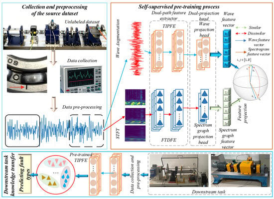
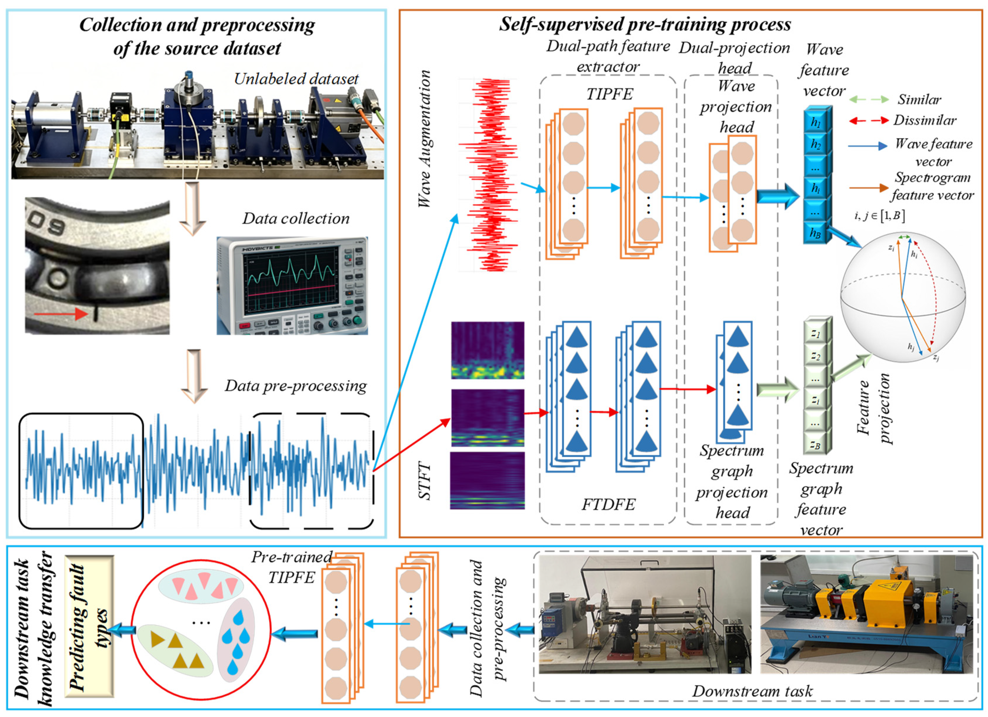
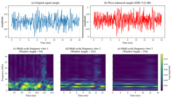
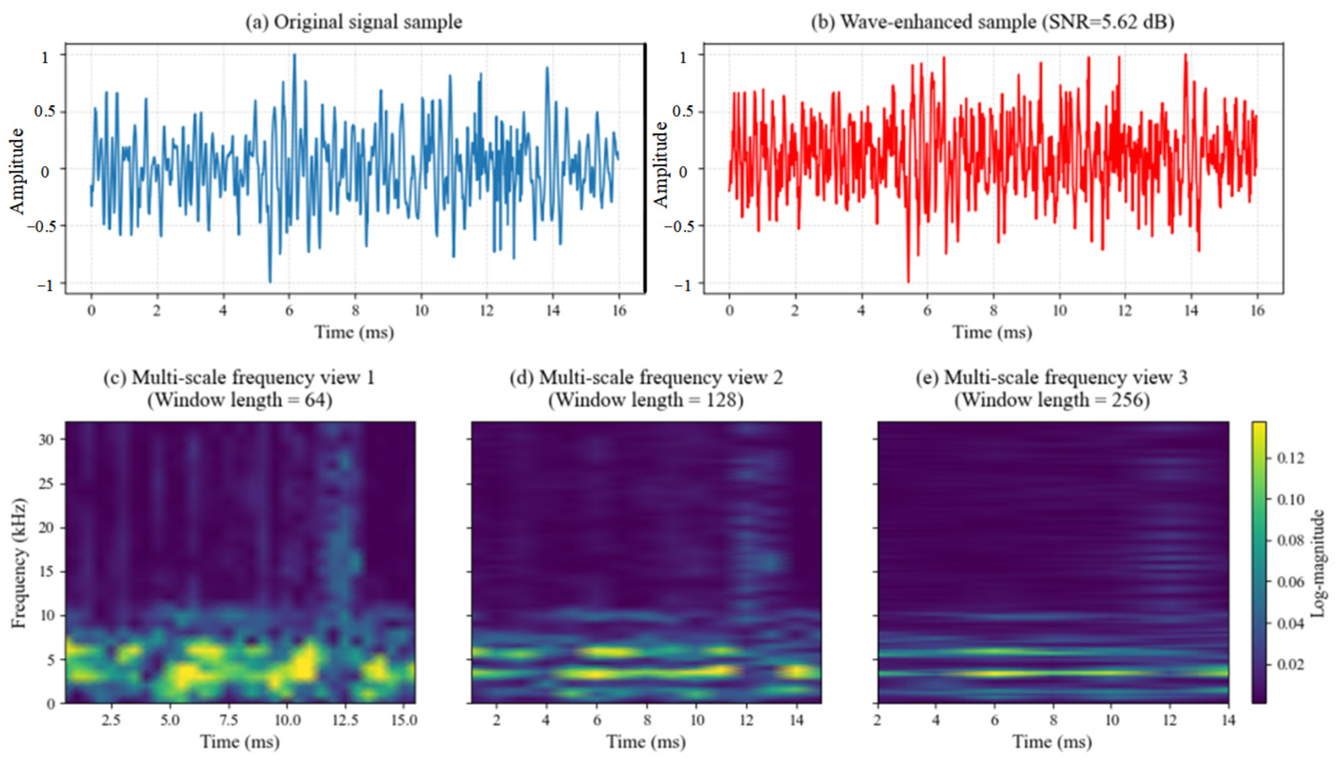
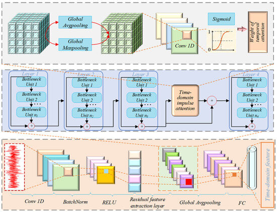
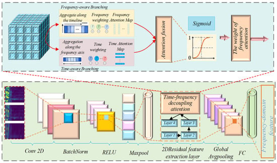
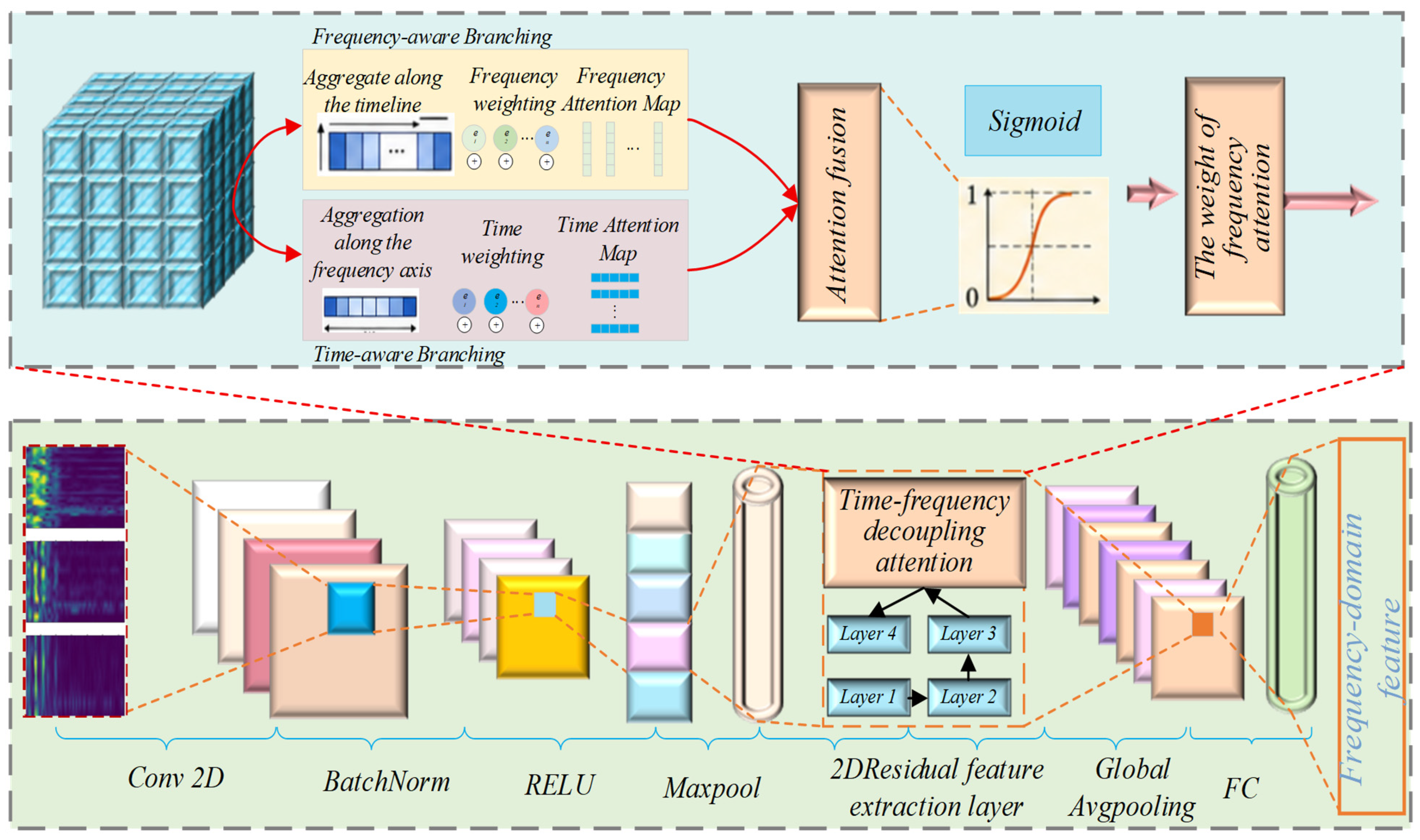
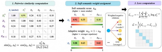
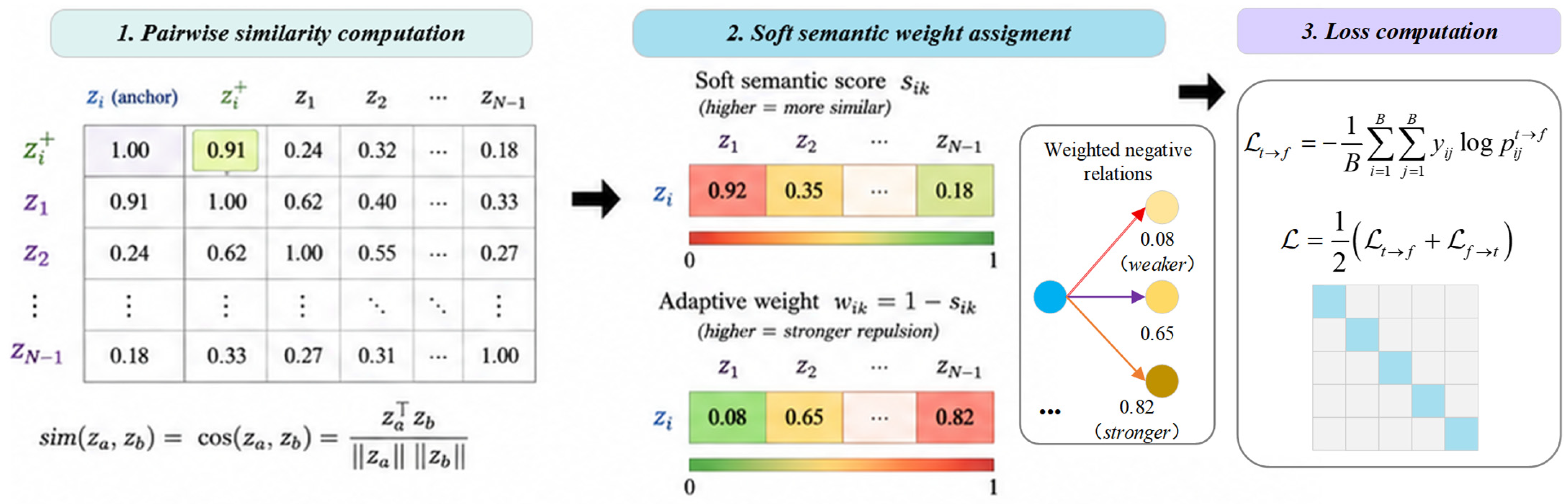
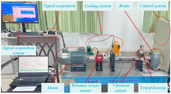
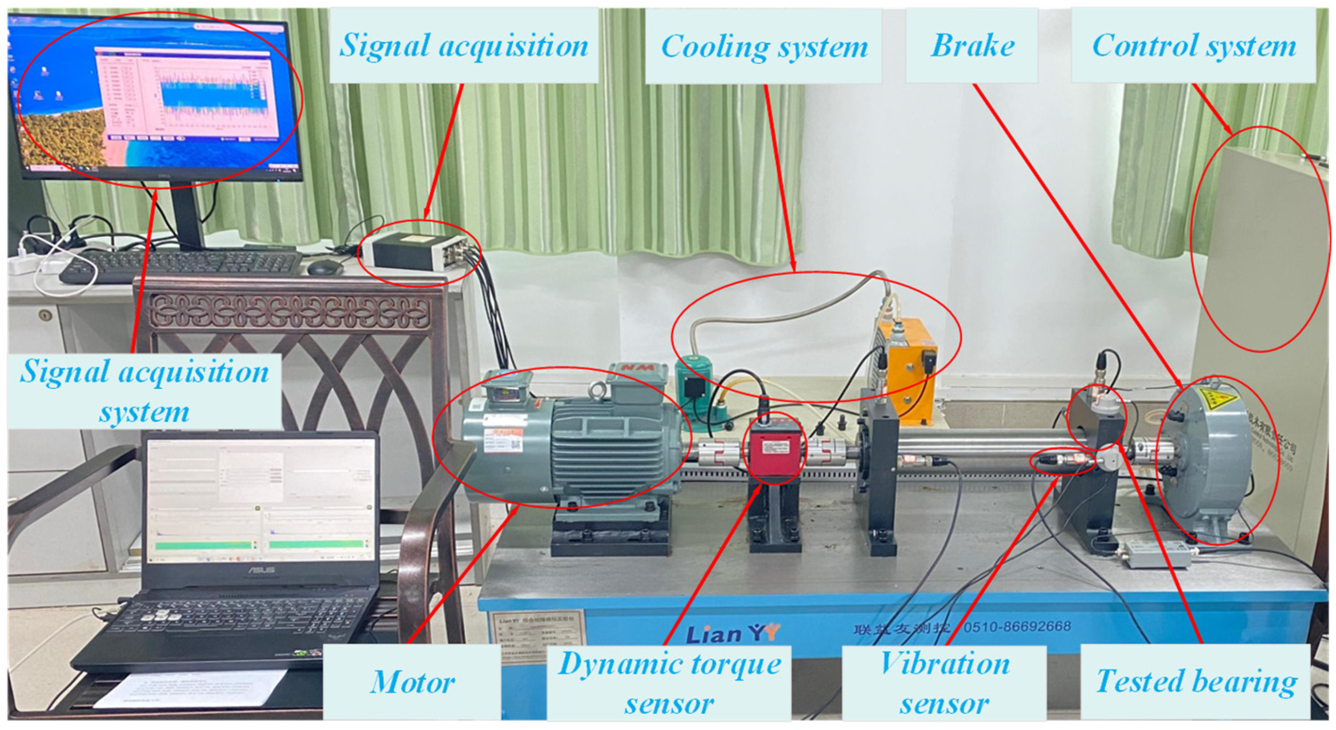
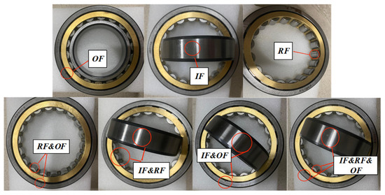
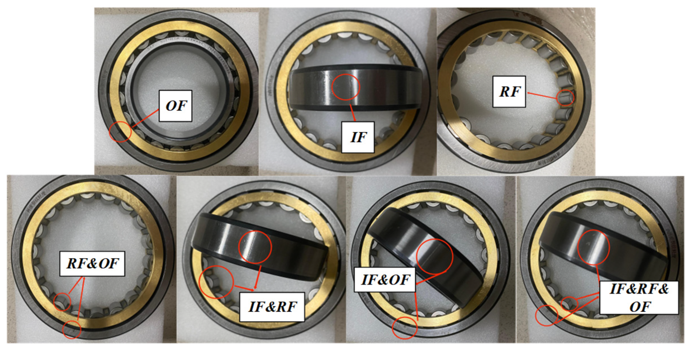
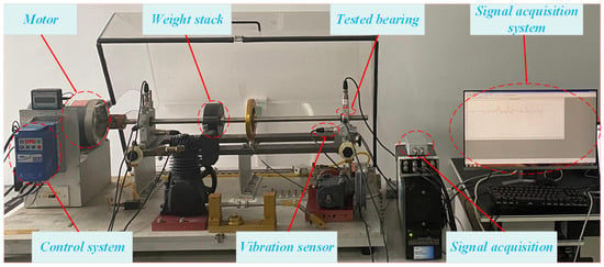
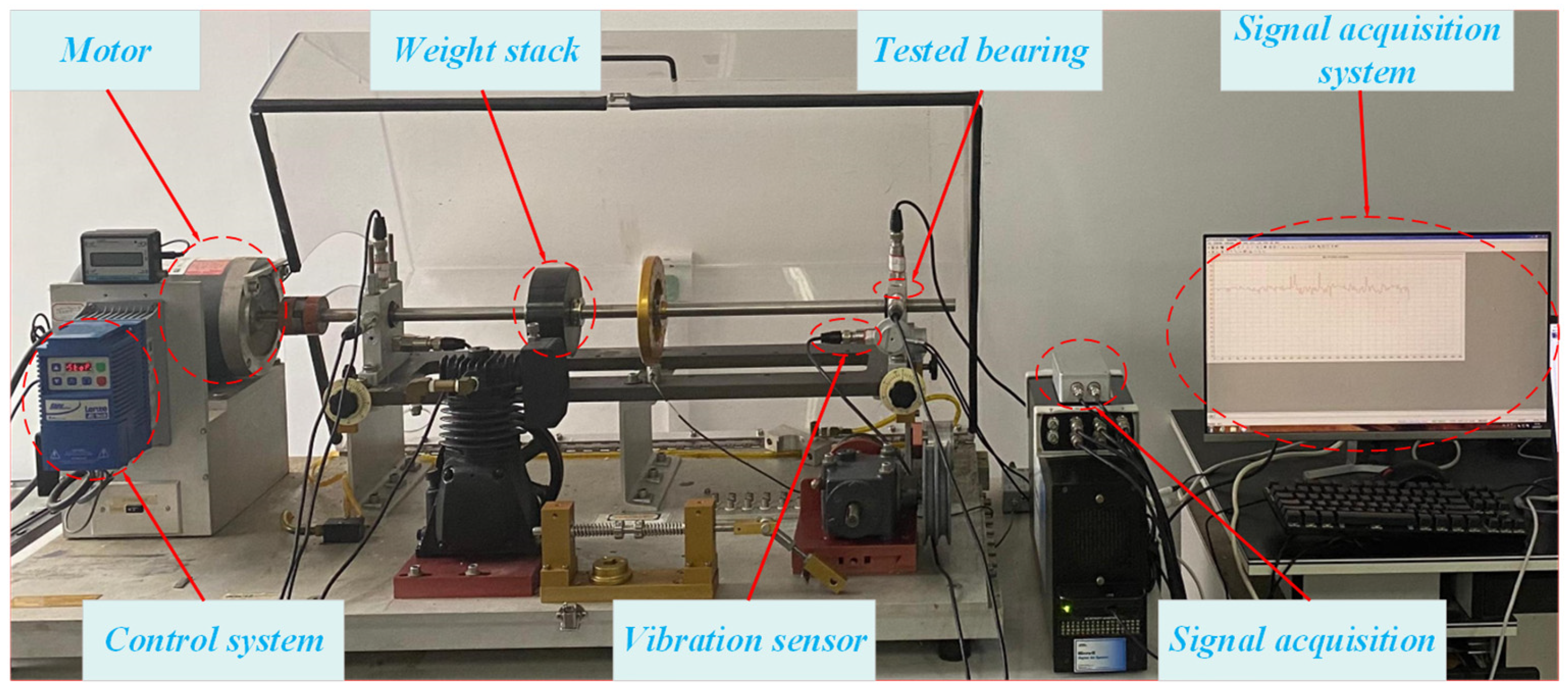
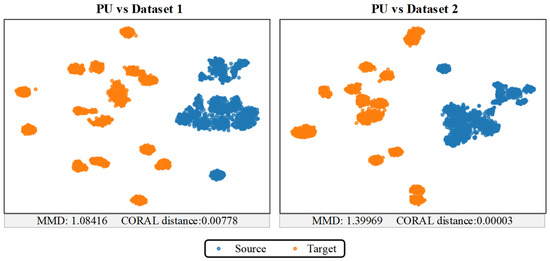
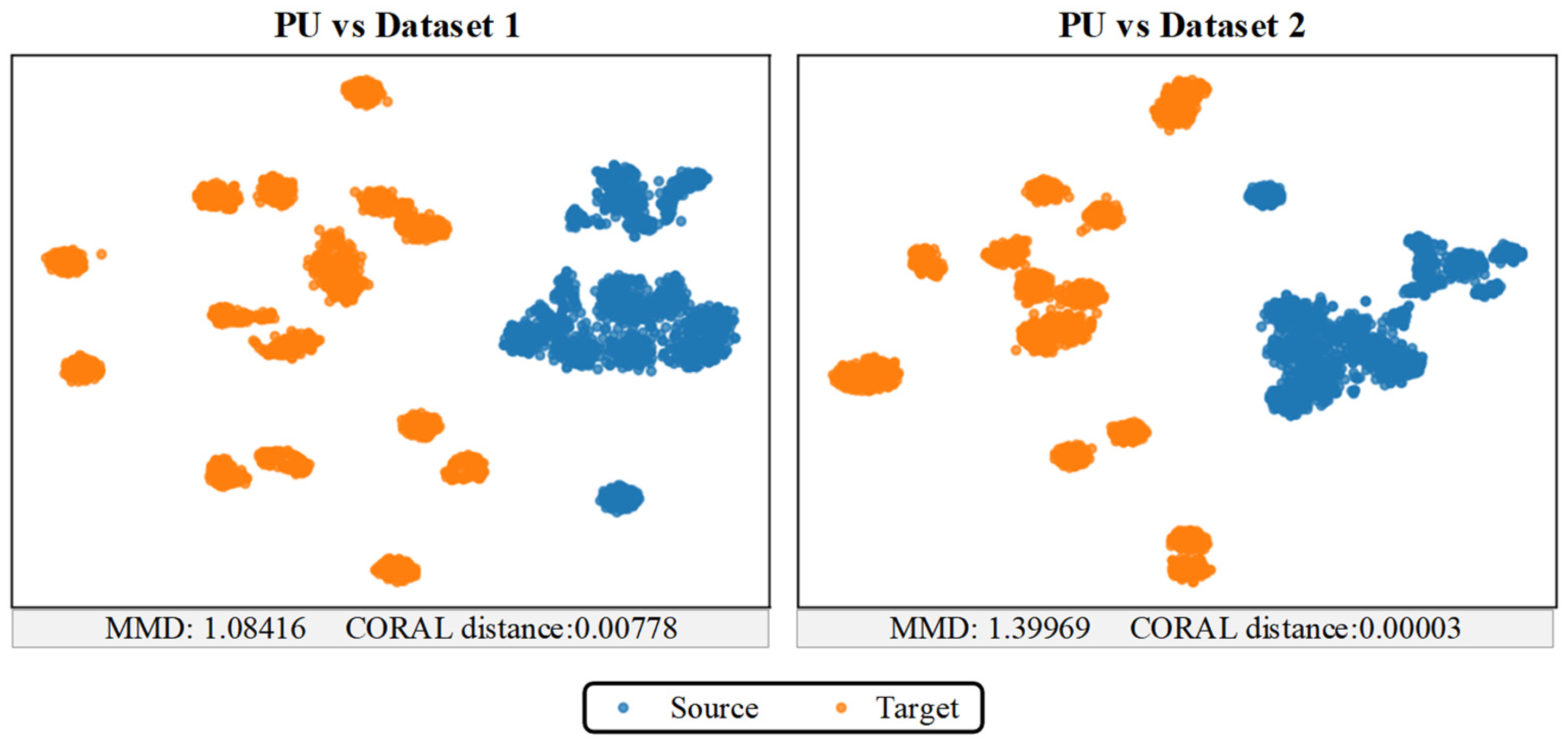
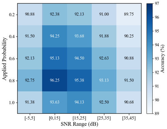
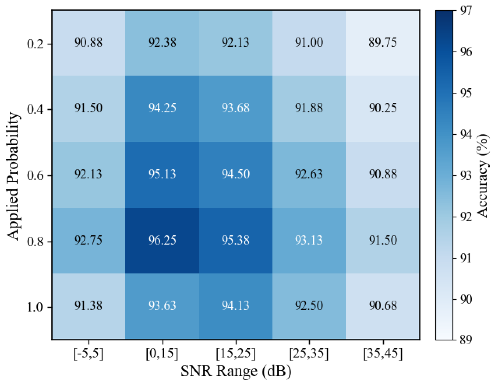
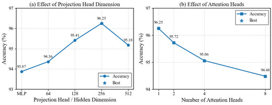
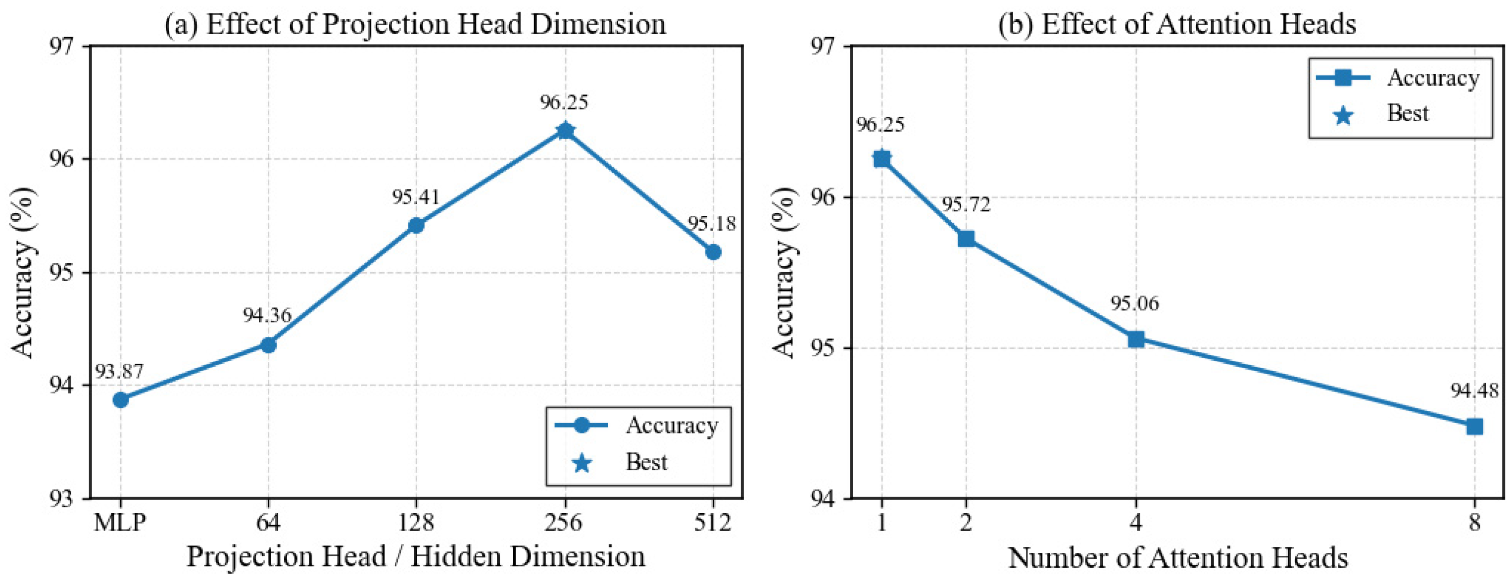
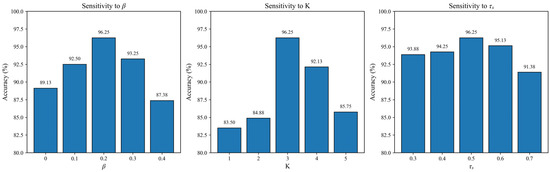
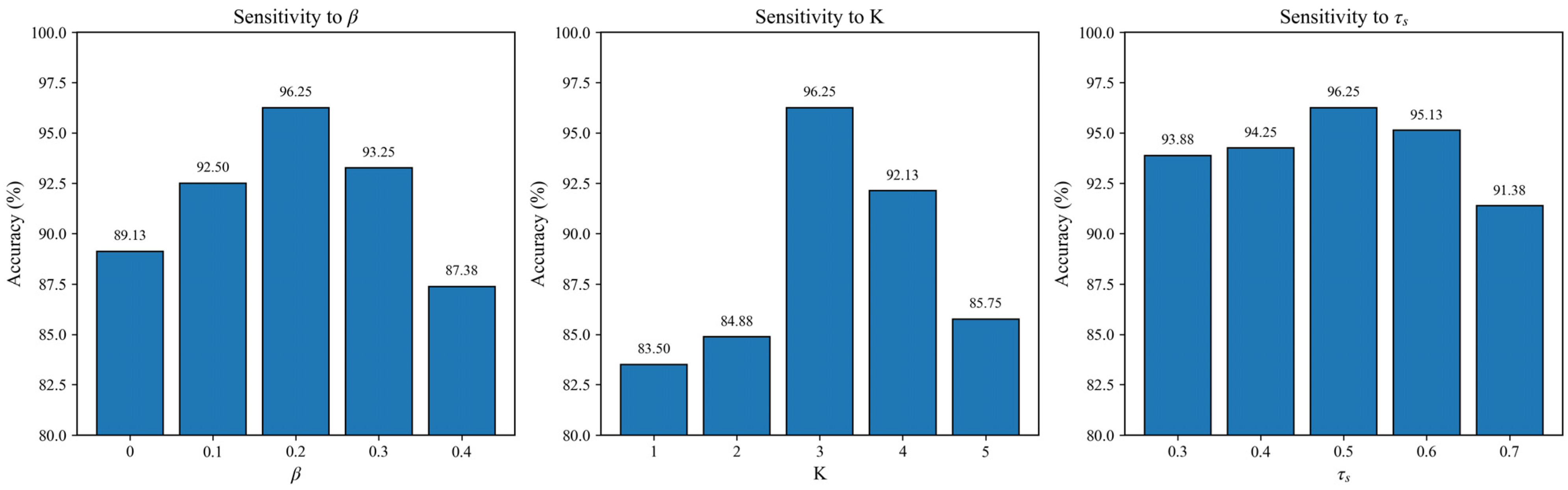
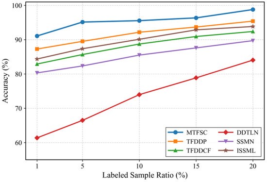
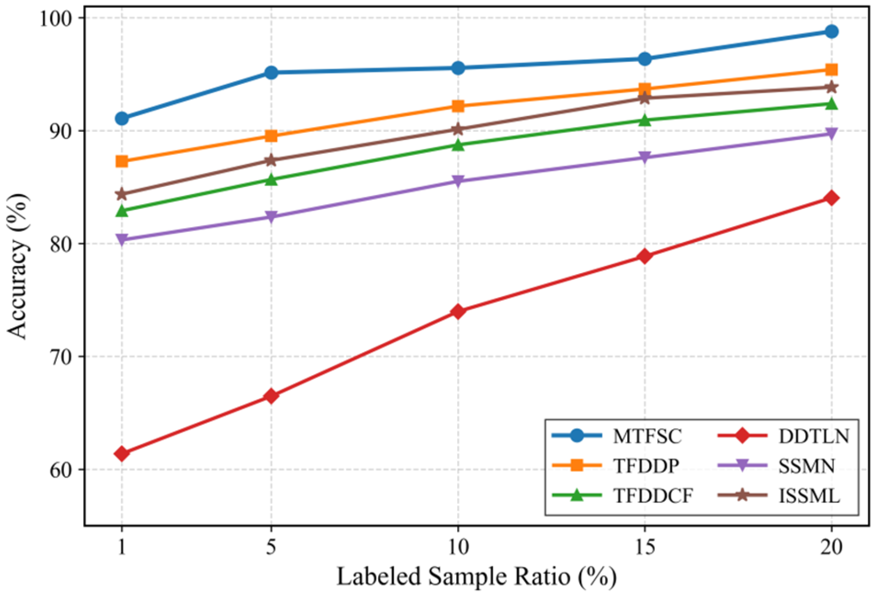
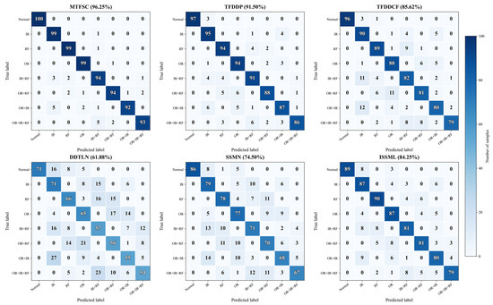
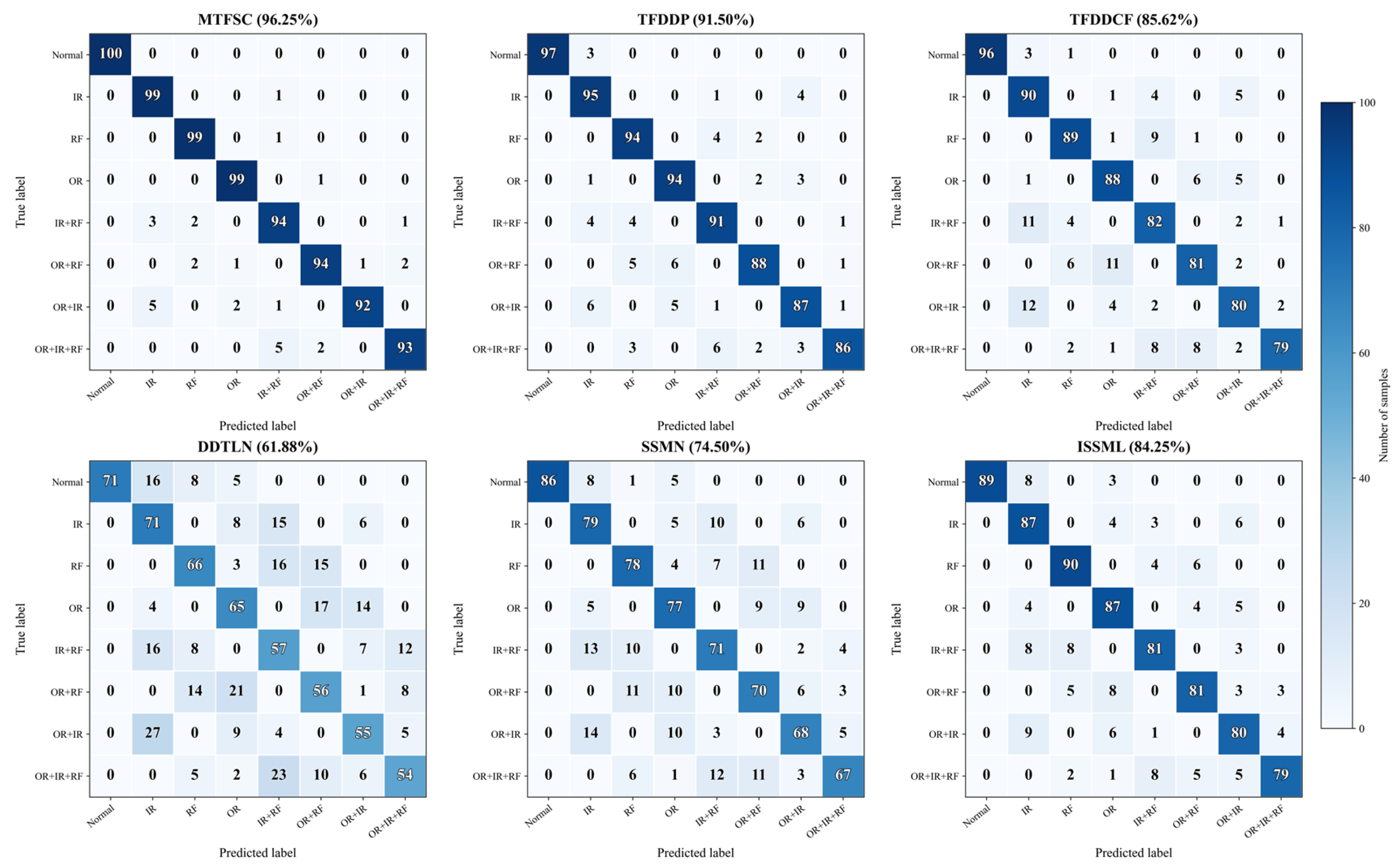

Disclaimer/Publisher’s Note: The statements, opinions and data contained in all publications are solely those of the individual author(s) and contributor(s) and not of MDPI and/or the editor(s). MDPI and/or the editor(s) disclaim responsibility for any injury to people or property resulting from any ideas, methods, instructions or products referred to in the content. |
© 2026 by the authors. Licensee MDPI, Basel, Switzerland. This article is an open access article distributed under the terms and conditions of the Creative Commons Attribution (CC BY) license.