On Iterative Algorithms with Different Mapping in Each Iteration

Abstract

Algorithm unrolling (unfolding) is a process where an existing iterative algorithm is converted into another iterative algorithm, but the mapping in each iteration of the new algorithm can potentially be different. An abstraction is to consider a sequence of mappings $T_m$, where each mapping potentially acts on a different metric space $(X_m,d_m)$. We study the iterates from the sequence of mappings and derive conditions for convergence. The first result is when both the mapping and metric space are different in each iteration. The second result is when all metric spaces are the same, but the mapping is different in each iteration. The second result can be considered as a generalization of the Banach Fixed Point theorem. A concrete practical example is the unrolling of the Iterative Shrinkage–Thresholding Algorithm, which has applications in statistics, machine learning and signal processing. The convergence of this example will be analyzed with the aid of the result established through this work.

1. Introduction

Recently there has been an increasing interest in developing AI (artificial intelligence) algorithms using the technique of algorithm unrolling [1]. The motivation behind algorithm unrolling is to achieve some interpretability in the AI algorithm, unlike many other AI algorithms which are usually considered ’black boxes’. The main idea with algorithm unrolling is the conversion of an iterative algorithm, e.g., Iterative Shrinkage–Thresholding Algorithm (ISTA) [2,3,4,5], into another iterative algorithm with a different mapping in each iteration. Algorithm unrolling has been successfully applied in applications such as compressed sensing [6], phase retrieval [7], power systems [8], image fusion [9] and microscopy [10]. The original iterative algorithm is usually derived from theoretical and/or physical consideration of the problem at hand. The unrolled algorithm inherits some of the theoretical and/or physical features from the original algorithm, and therefore has some aspects of interpretability. For example with ISTA, the theoretical consideration is to achieve a sparse representation of a signal vector given a dictionary of atom (constituent) vectors. An abstraction of algorithm unrolling is to consider a sequence of mappings between metric spaces, where the application of a mapping can be considered as one iteration of the algorithm. This abstraction is also relevant in other areas like non-autonomous contraction mappings [11].

Consider a sequence of metric spaces $(X_m,d_m)$, $m=0,1,2,\dots$, where $X_m$ denotes the set of elements (points) and $d_m(•,•)$ denotes the corresponding distance function. The sequence of mappings $T_m$ is between the metric spaces:

$$T_m:X_{m-1}\to X_m$$

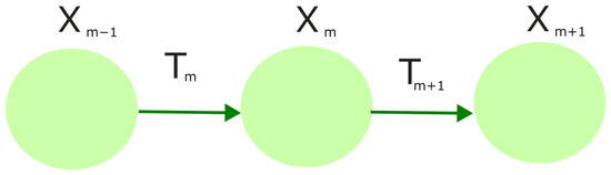
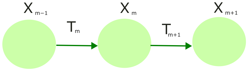
for $m=1,\dots$, as illustrated in Figure 1. Starting with an initial point $x^{\left(0\right)}\in X_0$, we consider the new point after the application of the sequence of mappings:

$$x^{\left(M\right)}=T_M\circ \dots \circ T_1\left(x^{\left(0\right)}\right)\in X_M,$$

(1)

where the symbol ‘∘’ denotes the composition of mappings. The superscript ‘$\left(m\right)$’ in $x^{\left(m\right)}$ denotes the index of the space the point belongs to, i.e., $x^{\left(m\right)}\in X_m$. However if the point is obtained using (1), m also represents the index of the term in the sequence. In other words, $x^{\left(m\right)}$ is the $m^{th}$ term in the sequence $x^{\left(0\right)},x^{\left(1\right)},\dots$, where every term in the sequence, in general, belongs to a different space.

Figure 1. Sequence of mappings between metric spaces.

When all metric spaces are the same, i.e., $X_m=X$, $\forall m$, and all mappings are the same, i.e., $T_m=T$, $\forall m$, (1) represents the classical iteration procedure found in many branches of applied mathematics and data science, e.g., Jacobi iterations and Gauss–Seidel iterations [12]. Furthermore, when the mapping T is a contraction, the Banach Fixed Point theorem applies, and this also has applications in the study of differential and integral equations [12].

In practice, with algorithm unrolling, the different mappings are obtained through parametrization; i.e., $T_m(•)=T(•;{\mathit{\kappa }}_m)$ where ${\mathit{\kappa }}_m$ is the parameter vector that defines the mapping in each iteration.

Sequences of contraction mappings have also previously been considered in [13,14,15,16]. However the context considered in [13,14,15,16] is different to that considered here. The works in [13,14,15,16] are mainly interested in the convergence of the sequence of fixed points from the sequence of contraction mappings $T_1,T_2,\dots$, i.e., the convergence of $x_n^{\ast }$ where $T_n\left(x_n^{\ast }\right)=x_n^{\ast }$. These previous works do not consider the tandem application of the sequence of mappings as shown in (1). In this work, we study the behavior of (1) as $M\to \infty$ and prove some convergence results. More detailed comparisons are deferred to Section 5. Application to the unrolled ISTA will also be considered. To the best of our knowledge, similar results are not found elsewhere.

Organization of paper: In Section 2, we review some definitions and concepts in metric spaces that are relevant to this work. New definitions which are generalizations of classical notions will also be presented here. The convergence in the general case, with different mappings and different metric spaces, is analyzed in Section 3. In Section 4, the convergence with different mappings on the same metric space is analyzed. Detailed comparisons with previous works, which considered sequences of mappings, are found in Section 5. The general convergence result is then used to analyze the convergence of the unrolled ISTA in Section 6. Concluding remarks are found in Section 7.

2. Preliminaries and Definitions

Firstly, we provide some comments about the notation used in the paper. As mentioned earlier, the superscript ‘$\left(m\right)$’ in $x^{\left(m\right)}$ denotes the index of the space the point belongs to, i.e., $x^{\left(m\right)}\in X_m$. In general, the spaces are different; i.e., $X_{m_1}\ne X_{m_2}$ for $m_1\ne m_2$. Since we are concerned with a sequence of mappings from one space to another space, m also represents the index of the sequence; i.e., $(x^{\left(0\right)},x^{\left(1\right)},\dots )$ represents a sequence of points in different spaces (in general). In the special case when all the spaces are the same, we use a subscript to denote the index of the sequence, i.e., $x_0,x_1,\dots$, which is the common convention for sequences.

We first recall some basic definitions for metric spaces [12] which are relevant to the developments that follow. A metric space is a set of points (elements) X and an endowed distance function $d(•,•)$ that satisfies the following axioms. For all $x,y,z\in X$, we have

A1 

$d(x,y)$ is a non-negative finite-valued function.

A2 

$d(x,y)=0$ if and only if $x=y$.

A3 

$d(x,y)=d(y,x)$; i.e., the distance function is symmetric.

A4 

$d(x,y)\le d(x,z)+d(z,y)$ which is known as the triangle inequality.

Using induction on axiom A4, we have the following.

Definition 1 (Generalized triangle inequality).

For all $x_1,x_2,\dots ,x_K\in X$,

$$d(x_1,x_K)\le {\displaystyle \sum _{k=1}^{K-1}}d(x_k,x_{k+1})$$

(2)

Definition 2 (Cauchy sequence and completeness).

A sequence $x_k\in X$ ($k=1,\dots$) is a Cauchy sequence if for every $ϵ>0$, there exists $K=K\left(ϵ\right)$ such that

$$d(x_{k_1},x_{k_2})<ϵfor every k_1,k_2>K\left(ϵ\right).$$

If every Cauchy sequence $x_k$ converges to a limit point, i.e.,

$$\underset{k\to \infty }{\lim }{x}_k=x_{\mathit{limit}},$$

then the space X is complete.

Consider a mapping $T:X⟶X$ which maps points in X onto itself. The mapping T is a contraction if there exists a constant $0<\widehat{\alpha }<1$ such that for all $x,y\in X$

$$d(T\left(x\right),T\left(y\right))\le \widehat{\alpha }d(x,y)$$

With a contraction mapping, we have the well-known Banach Fixed Point Theorem (BFPT).

Theorem 1 (BFPT).

Consider a complete metric space $(X,d)$ and a contraction mapping T: $X⟶X$. We have the following:

1. 

There exists a point $x^{\ast }\in X$ such that

$$T\left(x^{\ast }\right)=x^{\ast }.$$

The point $x^{\ast }$ is unique and is known as the fixed point of T.

2. 

Given any initial point $x_0\in X$, the sequence of points $x_1,x_2,\dots$ generated from the iterations

$$x_k=T\left(x_{k-1}\right)fork\ge 1$$

converges to a fixed point; i.e.,

$$\underset{k\to \infty }{\lim }{x}_k=x^{\ast }$$

The discussions above are for a single metric space and a single mapping. However, in this work we are considering the general case of multiple metric spaces and multiple mappings as described in (1). Some of the results above are still relevant, e.g., axioms A1–A4 and Definitions 1 and 2, when we are considering each metric space in the sequence in isolation. The relationships above will have superscript ^(m) for the elements of the metric space $X_m$ with the corresponding distance function $d_m$. However, new definitions are needed, when multiple metric spaces and mappings are involved.

Definition 3 (Lipschitz coefficient).

For the map $T_m:X_{m-1}\to X_m$, let

$$S_m\equiv \{(x_A^{(m-1)},x_B^{(m-1)}):x_A^{(m-1)}\ne x_B^{(m-1)},x_A^{(m-1)},x_B^{(m-1)}\in X_{m-1}\}.$$

The coefficient ${\alpha }_m$ of the map is defined as

$${\alpha }_m\equiv \underset{S_m}{\sup }{\displaystyle \frac{d_m(T_m(x_A^{(m-1)}),T_m(x_B^{(m-1)}))}{d_{m-1}(x_A^{(m-1)},x_B^{(m-1)})}}$$

Note that since $x_A^{(m-1)}\ne x_B^{(m-1)}$, by axiom A2, the denominator is non-zero. If $T_m$ is a trivial constant map, then the numerator and ${\alpha }_m$ are equal to zero. We only consider non-trivial maps such that ${\alpha }_m$ is positive. If ${\alpha }_m$ is finite-valued, we have the following inequality:

$$d_m(T_m\left(x_A^{(m-1)}\right),T_m\left(x_B^{(m-1)}\right))\le {\alpha }_m{d}_{m-1}(x_A^{(m-1)},x_B^{(m-1)})$$

(3)

Note that when $x_A^{(m-1)}=x_B^{(m-1)}$, $T_m\left(x_A^{(m-1)}\right)=T_m\left(x_B^{(m-1)}\right)$, and both sides of (3) are equal to zero; i.e., (3) is still valid.

Definition 4 (Contraction mapping).

The (non-trivial) mapping $T_m$ is a contraction if $0<{\alpha }_m<1$ and we have

$$\begin{array}{ccc}\hfill d_m(T_m\left(x_A^{(m-1)}\right),T_m\left(x_B^{(m-1)}\right))& \le & {\alpha }_m{d}_{m-1}(x_A^{(m-1)},x_B^{(m-1)})\hfill \\ & \le & d_{m-1}(x_A^{(m-1)},x_B^{(m-1)})\hfill \end{array}$$

(4)

$\forall x_A^{(m-1)},x_B^{(m-1)}\in X_{m-1}$.

Definitions 3 and 4 are generalizations of the classical notions in a single metric space and mapping to sequences of metric spaces and mappings. Note that inequality (3) applies to any mapping $T_m$, but (4) applies only to mappings that are contractions.

3. Different Spaces and Different Mappings

Suppose we start the iterations in (1) with two different initial points $x_A^{\left(0\right)}\in X_0$ and $x_B^{\left(0\right)}\in X_0$. We have the following result.

Theorem 2. 

Suppose the mappings $T_m$ ($m=1,\dots$) satisfy the following conditions:

1. 

The Lipschitz coefficients ${\alpha }_m$ (for all m) are positive and finite; i.e., $0<{\alpha }_m<\infty$.

2. 

There exists a finite positive integer L such that

$$\widehat{\alpha }\equiv \underset{m\ge L}{\sup }{\alpha }_m\le c<1.$$

(5)

Then we have

$$\underset{M\to \infty }{\lim }{d}_M(x_A^{\left(M\right)},x_B^{\left(M\right)})=0$$

(6)

for any $x_A^{\left(0\right)}\in X_0$ and $x_B^{\left(0\right)}\in X_0$.

Proof. 

If $x_A^{\left(0\right)}=x_B^{\left(0\right)}$, then $x_A^{\left(m\right)}=x_B^{\left(m\right)}$ for all m, and (6) is satisfied. We then consider the general case when $x_A^{\left(0\right)}\ne x_B^{\left(0\right)}$. By definition

$$d_M(x_A^{\left(M\right)},x_B^{\left(M\right)})=d_M(T_M\left(x_A^{(M-1)}\right),T_M\left(x_B^{(M-1)}\right)).$$

Using inequality (3), we have

$$\begin{array}{ccc}\hfill d_M(x_A^{\left(M\right)},x_B^{\left(M\right)})& \le & {\alpha }_M{d}_{M-1}(x_A^{(M-1)},x_B^{(M-1)})\hfill \\ & =& {\alpha }_M{d}_{M-1}(T_{M-1}\left(x_A^{(M-2)}\right),T_{M-1}\left(x_B^{(M-2)}\right))\hfill \\ & \le & {\alpha }_M{\alpha }_{M-1}{d}_{M-2}(x_A^{(M-2)},x_B^{(M-2)})\hfill \\ & & ⋮\hfill \\ & \le & {\alpha }_M{\alpha }_{M-1}\dots {\alpha }_1{d}_0(x_A^{\left(0\right)},x_B^{\left(0\right)})\hfill \\ & =& \left({\displaystyle \prod _{k=L}^M}{\alpha }_k\right)\left({\displaystyle \prod _{k=1}^{L-1}}{\alpha }_k\right)d_0(x_A^{\left(0\right)},x_B^{\left(0\right)})\hfill \end{array}$$

(7)

Condition (5) implies that

$$0<{\alpha }_m\le \widehat{\alpha }<1\mathrm{for}m\ge L$$

(8)

Using (8) in (7), we have

$$\begin{array}{ccc}\hfill d_M(x_A^{\left(M\right)},x_B^{\left(M\right)})& \le & {\widehat{\alpha }}^{M-L+1}\left({\displaystyle \prod _{k=1}^{L-1}}{\alpha }_k\right)d_0(x_A^{\left(0\right)},x_B^{\left(0\right)})\hfill \\ & =& {\widehat{\alpha }}^M\underset{\equiv K(L,x_A^{\left(0\right)},x_B^{\left(0\right)})}{\underbrace{{\widehat{\alpha }}^{-L+1}\left(\prod _{k=1}^{L-1}{\alpha }_k\right)d_0(x_A^{\left(0\right)},x_B^{\left(0\right)})}}\hfill \end{array}$$

$$\therefore d_M(x_A^{\left(M\right)},x_B^{\left(M\right)})\le {\widehat{\alpha }}^{M}K(L,x_A^{\left(0\right)},x_B^{\left(0\right)})$$

(9)

Now $K(L,x_A^{\left(0\right)},x_B^{\left(0\right)})$ consists of a finite product of the terms involving $\widehat{\alpha }$, ${\alpha }_k$ and $d_0(x_A^{\left(0\right)},x_B^{\left(0\right)})$. Since $\widehat{\alpha }$, ${\alpha }_k$ and $d_0(x_A^{\left(0\right)},x_B^{\left(0\right)})$ are all finite, $K(L,x_A^{\left(0\right)},x_B^{\left(0\right)})$ will also be finite. As a consequence of (8), the term ${\widehat{\alpha }}^M$ can be made arbitrarily small by choosing a sufficiently large M; i.e.,

$$\underset{M\to \infty }{\lim }{\widehat{\alpha }}^M=0.$$

Therefore we have (6). □

Remark 1. 

1. 

Theorem 2 shows that not every mapping needs to be contractive for convergence. As long as the mappings become contractive after a finite number of iterations, convergence is achieved.

2. 

It is important to note that, starting from an initial point $x_A^{\left(0\right)}$, the iterates do not necessarily converge to a limit point. Rather, the initial point is immaterial, after a sufficiently large number of iterations, to the eventual sequence of iterates; i.e., $x_A^{\left(M\right)}\approx x_B^{\left(M\right)}$ for large M—trajectory convergence. This is useful, from a practical perspective, as one does not need to be too concerned with the initialization of the iterative algorithm, as long as there is a sufficient number of iterations.

3. 

Note that, since the iterates $x^{\left(m\right)}$ belong to different function spaces in general, the notion of a Cauchy sequence is not relevant here. In a Cauchy sequence (Definition 2), all terms belong to the same space. Even when all iterates belong to the same space, trajectory convergence does not imply convergence to a limit point—see the example below.

4. 

Conditions for convergence to a limit point are considered in Section 4.

Example 1.

Consider a simple example, where the metric space is the Banach space of vectors in $X_m={\mathbb{R}}^q$ (for all m), with the following mapping:

$$T_m\left(\mathbf{x}\right)=K{e}^{-\alpha m}\mathbf{x}+m^2\mathbf{1}$$

where $K>1$, $\alpha >0$ and $\mathbf{1}$ is the vector with all ones. We then have

$$d({\mathbf{x}}_m^A,{\mathbf{x}}_m^B)=\left|\right|K{e}^{-\alpha m}({\mathbf{x}}_{m-1}^A-{\mathbf{x}}_{m-1}^B)\left|\right|=K{e}^{-\alpha m}\left|\right|{\mathbf{x}}_{m-1}^A-{\mathbf{x}}_{m-1}^B\left|\right|=K{e}^{-\alpha m}d({\mathbf{x}}_{m-1}^A,{\mathbf{x}}_{m-1}^B)$$

For trajectory convergence, we require $K{e}^{-\alpha m}<1$, which is achieved when

$$m>{\displaystyle \frac{1}{\alpha }}\ln K$$

However, when we consider the difference between two successive iterates, we have

$${\mathbf{x}}_m-{\mathbf{x}}_{m-1}=(K{e}^{-\alpha m}-1){\mathbf{x}}_{m-1}+m^2\mathbf{1}$$

As $m\to \infty$, $\left|\right|{\mathbf{x}}_m-{\mathbf{x}}_{m-1}\left|\right|$ does not approach zero; i.e., the sequence is not Cauchy and does not converge to a limit point.

When all mappings are contractions ($L=1$), a simple formula for estimating the number of iterations to achieve a prescribed error is given by the following.

Corollary 1. 

If all conditions of Theorem 2 are satisfied, when $L=1$, for a given $\epsilon \in (0,d_0(x_A^{\left(0\right)},x_B^{\left(0\right)}))$, the bound

$$d_M(x_A^{\left(M\right)},x_B^{\left(M\right)})\le \epsilon$$

is achieved if the number of iterations M satisfies

$$M\ge {\displaystyle \frac{\log (\epsilon /D_0)}{\log \widehat{\alpha }}},$$

(10)

where

$$D_0\equiv d_0(x_A^{\left(0\right)},x_B^{\left(0\right)})and\widehat{\alpha }\equiv \underset{m}{\sup }{\alpha }_m<1.$$

Proof. 

Using (9) with $L=1$, we require

$$d_M(x_A^{\left(M\right)},x_B^{\left(M\right)})\le {\widehat{\alpha }}^M{D}_0\le \epsilon$$

$$⟹{\widehat{\alpha }}^M\le \epsilon /D_0$$

Taking the logarithm (of any base) of both sides, and noting that $\log (\epsilon /D_0)<0$ and $\log \widehat{\alpha }<0$, so that the inequality is reversed, we have

$$M\log \widehat{\alpha }\ge \log (\epsilon /D_0)$$

Inequality (10) is then obtained. □

4. Different Mappings on the Same Metric Space

We now consider the case where all spaces are the same; i.e., $X_m=X$, for all m and $T_m:X\to X$. Since all points are now in the same space, we denote the sequence $x^{\left(0\right)},x^{\left(1\right)},\dots$ (from the iterations) as $x_0,x_1,\dots$, where

$$x_m=T_m\left(x_{m-1}\right)\in X,\mathrm{for} \mathrm{all}m\ge 1.$$

(11)

Two new definitions, pertaining to the properties of the mappings, are first given.

Definition 5 (Pairwise contraction).

A pair of mappings $(T_p,T_q)$ is a pairwise contraction if for any $x_A,x_B\in X$ such that $x_A\ne x_B$, there exists a positive constant ${\tilde{\gamma }}_{p,q}<1$ such that

$$d(T_p\left(x_A\right),T_q\left(x_B\right))\le {\tilde{\gamma }}_{p,q}d(x_A,x_B)<d(x_A,x_B)$$

For a sequence of mappings $(T_1,T_2,\dots )$, we define the sequence of Lipschitz coefficients ${\gamma }_m$ ($m=1,\dots$) as

$${\gamma }_m\equiv \underset{\tilde{S}}{\sup }{\displaystyle \frac{d(T_{m+1}\left(x_A\right),T_m\left(x_B\right))}{d(x_A,x_B)}}$$

where

$$\tilde{S}\equiv \{(x_A,x_B):x_A\ne x_B,x_A\in X,x_B\in X\}$$

Definition 6 (Sequential contraction).

A sequence of mappings $T_1,T_2,\dots$ is a sequential contraction if the following conditions hold:

1. 

The sequence of Lipschitz coefficients ${\gamma }_m$ ($m=1,\dots$) are positive and finite-valued; i.e., $0<{\gamma }_m<\infty$.

2. 

There exists a finite positive integer L such that $(T_{m+1},T_m)$ is a pairwise contraction for all $m\ge L$; i.e.,

$$d(T_{m+1}\left(x_A\right),T_m\left(x_B\right))\le {\gamma }_{m}d(x_A,x_B)<d(x_A,x_B)$$

(12)

for any $x_A,x_B\in X$ such that $x_A\ne x_B$, and $0<{\gamma }_m<1$.

Remark 2. 

1. 

The definition above reduces to the classical definition of a contraction mapping if all the mappings are the same; i.e., $T_m=T$.

2. 

If T is a contraction mapping (in the classical sense), then $(T,T)$ is a pairwise contraction and the sequence $T,T,\dots$ is a sequential contraction.

We then have the following result.

Theorem 3. 

Consider the iterates from (11) on a complete metric space X. Suppose, for a given initial point $x_0$, the following conditions hold:

1. 

The sequence $T_1,T_2,\dots$ is a sequential contraction.

2. 

There exists a finite positive integer L such that

$$\widehat{\gamma }\equiv \underset{m\ge L}{\sup }{\gamma }_m\le c<1$$

(13)

3. 

$x_m\ne x_{m-1}$ for $m\ge 1$.

Then, for any initial point $x_0\in X$ whose generated iterates satisfy $x_m\ne {\mathit{x}}_{m-1}$, for all $m\ge 1$, there exists a limit point $x_{limit}\in X$ such that

$$\underset{M\to \infty }{\lim }{x}_M=x_{limit}⟺\underset{M\to \infty }{\lim }d(x_M,x_{limit})=0$$

Proof. 

Since ${\gamma }_m$ is positive and finite, we have

$$d(T_{m+1}\left(x_A\right),T_m\left(x_B\right))\le {\gamma }_{m}d(x_A,x_B)$$

(14)

for all $x_A,x_B\in X$ and $x_A\ne x_B$. For $m\ge L$, ${\gamma }_m<1$, and for $m<L$, ${\gamma }_m$ can be any finite positive value. Since $x_m\ne x_{m-1}$, using (14) repeatedly, we have

$$\begin{array}{ccc}\hfill d(x_{m+1},x_m)& =& d(T_{m+1}\left(x_m\right),T_m\left(x_{m-1}\right))\hfill \\ & \le & {\gamma }_{m}d(x_m,x_{m-1})\hfill \\ & \le & {\gamma }_m{\gamma }_{m-1}d(x_{m-1},x_{m-2})\hfill \\ & ⋮& \\ & \le & \left({\displaystyle \prod _{k=1}^m}{\gamma }_k\right)d(x_1,x_0)\hfill \\ & =& \left({\displaystyle \prod _{k=L}^m}{\gamma }_k\right)\left({\displaystyle \prod _{k=1}^{L-1}}{\gamma }_k\right)d(x_1,x_0)\hfill \end{array}$$

Using (13), for $k\ge L$ we have

$$0<{\gamma }_k\le \widehat{\gamma }<1$$

(15)

Therefore

$$\begin{array}{ccc}\hfill d(x_{m+1},x_m)& \le & {\widehat{\gamma }}^{m-L+1}\left({\displaystyle \prod _{k=1}^{L-1}}{\gamma }_k\right)d(x_1,x_0)\hfill \\ & =& {\widehat{\gamma }}^m\underset{\equiv \tilde{K}(L,x_1,x_0)}{\underbrace{{\widehat{\gamma }}^{-L+1}\left(\prod _{k=1}^{L-1}{\gamma }_k\right)d(x_1,x_0)}}\hfill \end{array}$$

$$\therefore d(x_{m+1},x_m)\le {\widehat{\gamma }}^m\tilde{K}(L,x_1,x_0)$$

(16)

Using the generalized triangle inequality (2), for $n>m\ge L$ we have

$$d(x_m,x_n)\le d(x_m,x_{m+1})+d(x_{m+1},x_{m+2})+\dots +d(x_{n-1},x_n)$$

Applying inequality (16) to each term on the R.H.S. we have

$$\begin{array}{ccc}\hfill d(x_m,x_n)& \le & {\widehat{\gamma }}^m\tilde{K}(L,x_1,x_0)+{\widehat{\gamma }}^{m+1}\tilde{K}(L,x_1,x_0)+\dots +{\widehat{\gamma }}^{n-1}\tilde{K}(L,x_1,x_0)\hfill \\ & =& ({\widehat{\gamma }}^m+{\widehat{\gamma }}^{m+1}+\dots +{\widehat{\gamma }}^{n-1})\tilde{K}(L,x_1,x_0)\hfill \end{array}$$

Applying the geometric series formula

$${\displaystyle \sum _{k=0}^{N-1}}a{r}^k={\displaystyle \frac{a(1-r^N)}{1-r}}$$

to the summation in brackets, where $a={\widehat{\gamma }}^m$, $r=\widehat{\gamma }$ and $N=n-m$, we have

$$d(x_m,x_n)\le {\widehat{\gamma }}^m{\displaystyle \frac{1-{\widehat{\gamma }}^{n-m}}{1-\widehat{\gamma }}}\tilde{K}(L,x_1,x_0)$$

Now (15) implies that $0<{\widehat{\gamma }}^{n-m}<1$ and therefore $0<1-{\widehat{\gamma }}^{n-m}<1$. Using this inequality we have

$$d(x_m,x_n)<{\widehat{\gamma }}^m{\displaystyle \frac{1}{1-\widehat{\gamma }}}\tilde{K}(L,x_1,x_0)$$

(17)

Now $\tilde{K}(L,x_1,x_0)$ is a finite product of terms involving $\widehat{\gamma }$, ${\gamma }_k$ and $d(x_1,x_0)$. Since the latter are all finite, $\tilde{K}(L,x_1,x_0)$ is also finite. The term ${\displaystyle \frac{1}{1-\widehat{\gamma }}}$ is positive and finite as $0<\widehat{\gamma }<1$. As a consequence of (15), ${\widehat{\gamma }}^m$ and therefore $d(x_m,x_n)$ can be made sufficiently small by choosing a sufficiently large m. This means that for every $\epsilon >0$, there exists a K such that

$$d(x_m,x_n)<\epsilon \mathrm{for} \mathrm{every}n>m>K,$$

meaning $x_1,x_2,\dots$ is a Cauchy sequence. Since the space X is complete, by Definition 2, a limit point exists. □

Remark 3. 

1. 

Although a limit point $x_{limit}$ exists, in general, $x_{limit}$ is not a fixed point of any of the mappings.

2. 

If all mappings are the same and are contractions, the conditions for the Banach Fixed Point theorem apply, and the limit point is also the fixed point of the mapping.

3. 

The limit point, in general, will depend on the initial point $x_0$.

A simple formula for estimating the number of required iterations, when $L=1$, is given by the following.

Corollary 2. 

If all conditions of Theorem 3 are satisfied, when $L=1$, for a given $\epsilon \in (0,d(x_1,x_0))$, the bound

$$d(x_M,x_{limit})<\epsilon$$

is achieved if the number of iterations M satisfies

$$M>{\displaystyle \frac{\log \left((1-\widehat{\gamma })\epsilon /{\tilde{D}}_0\right)}{\log \widehat{\gamma }}}$$

(18)

where

$${\tilde{D}}_0\equiv d(x_1,x_0)and\widehat{\gamma }\equiv \underset{m}{\sup }{\gamma }_m<1.$$

Proof. 

When $L=1$,

$$\tilde{K}(L,x_1,x_0)=d(x_1,x_0)={\tilde{D}}_0.$$

As $n\to \infty$, $x_n\to x_{limit}$. Therefore, using inequality (17), we have

$$d(x_M,x_{limit})<{\widehat{\gamma }}^M{\displaystyle \frac{1}{1-\widehat{\gamma }}}{\tilde{D}}_0<\epsilon$$

$$⟹{\widehat{\gamma }}^M<(1-\widehat{\gamma })\epsilon /{\tilde{D}}_0$$

Taking the logarithm (of any base) of both sides, and noting that $\log ((1-\widehat{\gamma })\epsilon /{\tilde{D}}_0)<0$ and $\log \widehat{\gamma }<0$, so that the inequality is reversed, we have

$$M\log \widehat{\gamma }>\log \left((1-\widehat{\gamma })\epsilon /{\tilde{D}}_0\right)$$

Inequality (18) is then obtained. □

5. Comparisons

Sequences of mappings have also been considered previously in [13,14,15,16]. We now make detailed comparisons with the previous works, and show that the previous results are fundamentally different to the results in this work.

The fundamental concept in previous works is to consider a sequence of self-mappings $T_n$ on a complete metric space X (with distance function d). The mappings are assumed to be contractions but with the possibility of different Lipschitz coefficients:

$$d(T_n\left(x\right),T_n\left(y\right))\le {\widehat{\alpha }}_{n}d(x,y)\mathrm{for} \mathrm{all}x,y\in X$$

where $0<{\widehat{\alpha }}_n<1$ for all n, and in general ${\widehat{\alpha }}_{n_1}\ne {\widehat{\alpha }}_{n_2}$ ($n_1\ne n_2$). By the Banach Fixed Point Theorem, there exists a unique fixed point for each $T_n$; i.e.,

$$T_n\left(x_n^{\ast }\right)=x_n^{\ast }\mathrm{for} \mathrm{all} n$$

The condition imposed on the sequence of mappings is that there exists a limiting self-map T, which is a contraction, such that

$$\underset{n\to \infty }{\lim }{T}_n\left(x\right)=T\left(x\right)\mathrm{for} \mathrm{all} x\in X$$

(19)

The convergence can be pointwise or uniform over X. Then the sequence of fixed points $x_n$ also converges to the fixed point of T; i.e.,

$$\underset{n\to \infty }{\lim }{x}_n=x^{\ast }\mathrm{where}T\left(x^{\ast }\right)=x^{\ast }$$

(20)

The results above do not explicitly refer to any iteration process to obtain the fixed points. However, Theorem 1 implies that each fixed point $x_n^{\ast }$ can be obtained as follows. Given any initial point $x_{n,0}\in X$, we perform the following iterations:

$$x_{n,k}=T_n\left(x_{n,k-1}\right)\mathrm{for}k\ge 1$$

(21)

and

$$x_n^{\ast }=\underset{k\to \infty }{\lim }{x}_{n,k}$$

(22)

In (21) and (22), the subscript ‘k’ tracks the iteration number, and the subscript ‘n’ tracks the mapping that is used. In general, a different initial point $x_{n,0}$ can be used for each mapping $T_n$. The important observation is that the same mapping is used for the iterations in (21). This is fundamentally different to (11) where, in general, a different mapping is used in each iteration. The condition for convergence in (20) is the existence of a limiting map as shown in (19), but no such condition is needed for (11). Although the limit point exists in both cases, the limit point from (11) is, in general, not associated with any fixed point of the maps, unlike in (19) where the limit point is also the fixed point of the map. Furthermore, not all maps with (11) need to be contractions; only maps after a finite number of iterations need to be contractions. However, all maps in (19) are contractions.

From an application perspective, the scenario described above—where there are multiple iterative algorithms as implied in (21) (one for each n)—is not something typically found in practice. Equations (19) and (20) are therefore primarily of theoretical interest. The iterations in (1), however, are found in practice, e.g., algorithm unrolling, and we will next study a concrete practical example.

6. Unrolled ISTA Algorithm

We now analyze the convergence of a well-known iterative algorithm with the aid of the previous result. The relevant metric space is the Banach space of vectors in ${\mathbb{R}}^q$ with the ${\mathcal{\ell }}^2$ distance function

$$d({\mathit{x}}_A,{\mathit{x}}_B)=\left|\right|{\mathit{x}}_A-{\mathit{x}}_B{\left|\right|}_2\equiv {\left({\displaystyle \sum _{k=1}^q}{({\mathit{x}}_A\left(k\right)-{\mathit{x}}_B\left(k\right))}^2\right)}^{1/2}.$$

The conventional Iterative Shrinkage–Thresholding Algorithm (ISTA) [2,3] can be described by the following iterations:

$${\mathit{x}}_m=S_{\beta }\left(\left(\mathit{I}-{\displaystyle \frac{1}{\mu }}{\mathit{W}}^T\mathit{W}\right){\mathit{x}}_{m-1}+{\displaystyle \frac{1}{\mu }}{\mathit{W}}^T\mathit{y}\right)$$

(23)

where $\beta ,\mu \in {\mathbb{R}}^{+}$ and $\mathit{W}\in {\mathbb{R}}^{p\times q}$ are parameters of the algorithm and $\mathit{y}\in {\mathbb{R}}^p$ is the given input. The soft thresholding function $S_{\beta }$ is applied element-wise to vectors in ${\mathbb{R}}^q$, and for a scalar $b\in \mathbb{R}$, is defined as

$$S_{\beta }\left(b\right)\equiv \left\{\begin{array}{cc}b-\beta \hfill & b>\beta \\ 0\hfill & -\beta \le b\le \beta \\ b+\beta \hfill & b<-\beta \end{array}\right.$$

(24)

Starting with an initial point ${\mathit{x}}_0\in {\mathbb{R}}^q$, a sequence of iterates ${\mathit{x}}_1,{\mathit{x}}_2,\dots \in {\mathbb{R}}^q$ is computed using (23). The algorithm arises in the context of LASSO (least absolute shrinkage and selection operator) in statistics and sparse coding in signal processing. In sparse coding, given an input $\mathit{y}$, the goal is to find a parsimonious representation of $\mathit{y}$ using an overcomplete dictionary of vectors, which are columns of $\mathit{W}$. A common approach to achieve this is to solve the following convex optimization problem:

$$\underset{\mathit{x}}{\min }\left\{\frac{1}{2}\left|\right|\mathit{y}-{\mathit{W}\mathit{x}\left|\right|}_2^2+{\beta \left|\right|\mathit{x}\left|\right|}_1\right\}$$

(25)

where $\beta$ is the regularization parameter that controls the level of sparsity. The solution to (25) can be achieved using the iterations in (23), where the parameter $\mu$ is the iteration step size.

The unrolled ISTA [1], by generalizing (23), is given by

$${\mathit{x}}_m=S_{{\beta }_m}\left({\mathit{X}}_m{\mathit{x}}_{m-1}+{\mathit{Y}}_m\mathit{y}\right)\equiv T_m({\mathit{x}}_{m-1};{\beta }_m,{\mathit{X}}_m,{\mathit{Y}}_m)$$

(26)

where the parameters of the mappings are ${\beta }_m$, ${\mathit{X}}_m$ and ${\mathit{Y}}_m$. When the parameters ${\beta }_m$, ${\mathit{X}}_m$ and ${\mathit{Y}}_m$ are determined via a machine learning framework, i.e., data-driven, we have what is commonly known as Learned ISTA or LISTA.

We will establish conditions for the convergence of (26). We first prove a relevant property of the soft thresholding function.

Lemma 1. 

The function $S_{\beta }\left(b\right)$ is  non-expansive  for any $\beta \in {\mathbb{R}}^{+}$; i.e.,

$$\left|\right|S_{\beta }\left({\mathit{z}}_1\right)-S_{\beta }\left({\mathit{z}}_2\right){\left|\right|}_2\le \left|\right|{\mathit{z}}_1-{\mathit{z}}_2{\left|\right|}_2$$

(27)

for all ${\mathit{z}}_1,{\mathit{z}}_2\in {\mathbb{R}}^q$.

Proof. 

We first establish the scalar form of (27). For any $b_1,b_2\in \mathbb{R}$, define

$${\Delta }_1\equiv |b_1-b_2|;{\Delta }_2\equiv |S_{\beta }\left(b_1\right)-S_{\beta }\left(b_2\right)|.$$

Due to the piece-wise nature of $S_{\beta }\left(b\right)$, as shown in (24), there are four cases to consider:

1.

For $-\beta \le b_1,b_2\le \beta$:

$$S_{\beta }\left(b_1\right)=S_{\beta }\left(b_2\right)=0.$$

Therefore ${\Delta }_2=0$ and since ${\Delta }_1\ge 0$, we have ${\Delta }_2\le {\Delta }_1$.

2.

For $-\beta \le b_1\le \beta$, $b_2>\beta$:

$$S_{\beta }\left(b_1\right)=0\mathrm{and}{S}_{\beta }\left(b_2\right)=b_2-\beta >0.$$

Therefore ${\Delta }_2=b_2-\beta$. Since $-\beta \le b_1\le \beta$,

$${\Delta }_2=b_2-\beta \le b_2-b_1={\Delta }_1.$$

Due to symmetry, this case is similar to the $-\beta \le b_2\le \beta$, $b_1>\beta$ case.

3.

For $b_1,b_2>\beta$:

$$S_{\beta }\left(b_1\right)=b_1-\beta >0\mathrm{and}{S}_{\beta }\left(b_2\right)=b_2-\beta >0.$$

Therefore

$${\Delta }_2=|b_1-b_2|={\Delta }_1.$$

Due to symmetry, this case is similar to the $b_1,b_2<-\beta$ case.

4.

For $b_1>\beta$, $b_2<-\beta$:

$$S_{\beta }\left(b_1\right)=b_1-\beta >0;S_{\beta }\left(b_2\right)=b_2+\beta <0\mathrm{and}{b}_1-b_2>0.$$

Therefore

$${\Delta }_2= |b_1-b_2-2\beta | < |b_1-b_2| ={\Delta }_1.$$

Due to symmetry, this case is similar to the $b_2>\beta$, $b_1<-\beta$ case.

Therefore, for all $b_1,b_2\in \mathbb{R}$, we have

$$\begin{array}{ccc}\hfill {\left({\Delta }_2\right)}^2& =& {(S_{\beta }\left(b_1\right)-S_{\beta }\left(b_2\right))}^2\hfill \\ & \le & {(b_1-b_2)}^2={\left({\Delta }_1\right)}^2\hfill \end{array}$$

(28)

Now consider the square of the L.H.S. of (27). Using (28), we have

$$\begin{array}{ccc}\hfill \left|\right|S_{\beta }\left({\mathit{z}}_1\right)-S_{\beta }\left({\mathit{z}}_2\right){\left|\right|}_2^2& =& {\displaystyle \sum _{k=1}^q}{(S_{\beta }\left({\mathit{z}}_1\left(k\right)\right)-S_{\beta }\left({\mathit{z}}_2\left(k\right)\right))}^2\hfill \\ & \le & {\displaystyle \sum _{k=1}^q}{({\mathit{z}}_1\left(k\right)-{\mathit{z}}_2\left(k\right))}^2\hfill \\ & =& \left|\right|{\mathit{z}}_1-{\mathit{z}}_2{\left|\right|}_2^2\hfill \end{array}$$

Taking the square root yields the desired result. □

The induced/operator norm is defined as

$$\left|\right|{\mathit{X}}_m{\left|\right|}_2\equiv \underset{\mathit{x}\ne \mathbf{0};\mathit{x}\in {\mathbb{R}}^q}{\sup }{\displaystyle \frac{\left|\right|{\mathit{X}}_m\mathit{x}{\left|\right|}_2}{{\left|\right|\mathit{x}\left|\right|}_2}},$$

which is also the spectral norm. The convergence of the unrolled ISTA is given by the following.

Theorem 4. 

Consider two initial points ${\mathit{x}}_0^A\in {\mathbb{R}}^q$ and ${\mathit{x}}_0^B\in {\mathbb{R}}^q$, and the corresponding iterates, ${\mathit{x}}_m^A\in {\mathbb{R}}^q$ and ${\mathit{x}}_m^B\in {\mathbb{R}}^q$, respectively, using (26). Suppose the parameters of the mappings $T_m$ satisfy the following conditions:

1. 

$\left|\right|{\mathit{X}}_m{\left|\right|}_2$ is positive and finite-valued for all m.

2. 

There exists a finite positive integer L such that

$$\underset{m\ge L}{\sup }\left|\right|{\mathit{X}}_m{\left|\right|}_2\le c<1$$

(29)

We then have

$$\underset{m\to \infty }{\lim }\left|\right|{\mathit{x}}_m^A-{\mathit{x}}_m^B{\left|\right|}_2=0\Rightarrow {\mathit{x}}_m^A\approx {\mathit{x}}_m^B\mathit{for}\mathit{large}m$$

(30)

Proof. 

From (26), with the parameters of the mapping suppressed for brevity, we have $T_m\left(\mathit{x}\right)=S_{{\beta }_m}\left({\mathit{X}}_m\mathit{x}+{\mathit{Y}}_m\mathit{y}\right)$. For any two arbitrary points ${\mathit{x}}_a,{\mathit{x}}_b\in {\mathbb{R}}^q$, using (27), we have

$$\begin{array}{ccc}\hfill \left|\right|T_m\left({\mathit{x}}_a\right)-T_m\left({\mathit{x}}_b\right){\left|\right|}_2& =& \left|\right|S_{{\beta }_m}\left({\mathit{X}}_m{\mathit{x}}_a+{\mathit{Y}}_m\mathit{y}\right)-S_{{\beta }_m}\left({\mathit{X}}_m{\mathit{x}}_b+{\mathit{Y}}_m\mathit{y}\right){\left|\right|}_2\hfill \\ & \le & \left|\right|\left({\mathit{X}}_m{\mathit{x}}_a+{\mathit{Y}}_m\mathit{y}\right)-\left({\mathit{X}}_m{\mathit{x}}_b+{\mathit{Y}}_m\mathit{y}\right){\left|\right|}_2\hfill \\ & =& \left|\right|{\mathit{X}}_m({\mathit{x}}_a-{\mathit{x}}_b){\left|\right|}_2\hfill \end{array}$$

Using the definition of the operator norm on the last expression, we have

$$\left|\right|T_m\left({\mathit{x}}_a\right)-T_m\left({\mathit{x}}_b\right){\left|\right|}_2\le \left|\right|{\mathit{X}}_m{\left|\right|}_2\left|\right|{\mathit{x}}_a-{\mathit{x}}_b{\left|\right|}_2$$

The Lipschitz coefficients are then ${\alpha }_m=\left|\right|{\mathit{X}}_m{\left|\right|}_2$ ($m=1,\dots$). By invoking Theorem 2, the required result is obtained. □

A special case of unrolling is when, instead of the generic ${\mathit{X}}_m$ in each iteration, we use a predetermined dictionary $\mathit{W}$, and allow the step size $\mu$ to vary between iterations. We then have the following corollary.

Corollary 3. 

Let ${\sigma }_{min}\left(\mathit{W}\right)$ and ${\sigma }_{max}\left(\mathit{W}\right)$ denote, respectively, the smallest and largest singular value of $\mathit{W}$. Suppose

$${\mathit{X}}_m=\left(\mathit{I}-{\displaystyle \frac{1}{{\mu }_m}}{\mathit{W}}^T\mathit{W}\right),$$

(31)

and the following conditions are satisfied:

1. 

The matrix $\mathit{W}$ has full column rank, so that ${\mathit{W}}^T\mathit{W}$ is positive definite, with singular values that satisfy

$$0<{\sigma }_{min}\left(\mathit{W}\right)<{\sigma }_{max}\left(\mathit{W}\right)<\infty .$$

(32)

2. 

There exists a small positive ϵ ($0<ϵ<<1$) such that

$${\displaystyle \frac{{\sigma }_{max}^2\left(\mathit{W}\right)}{2-ϵ}}<{\mu }_m<{\displaystyle \frac{{\sigma }_{min}^2\left(\mathit{W}\right)}{ϵ}}$$

(33)

for all m.

Convergence in (30) is then achieved.

Proof. 

We will show that conditions 1 and 2 of Theorem 4 are satisfied. The theorem is then invoked to prove the corollary. Firstly, we have

$${\mathit{X}}_m^T=\left({\mathit{I}}^T-{\displaystyle \frac{1}{{\mu }_m}}{\left({\mathit{W}}^T\mathit{W}\right)}^T\right)=\left(\mathit{I}-{\displaystyle \frac{1}{{\mu }_m}}{\mathit{W}}^T\mathit{W}\right)={\mathit{X}}_m$$

This means that ${\mathit{X}}_m$ is symmetric and has real eigenvalues. Therefore, the singular value (${\sigma }_i$) squared is equal to the eigenvalue (${\lambda }_i$) squared; i.e., ${\sigma }_i^2\left({\mathit{X}}_m\right)={\lambda }_i^2\left({\mathit{X}}_m\right)$ and ${\sigma }_i\left({\mathit{X}}_m\right)=\left|{\lambda }_i\left({\mathit{X}}_m\right)\right|$. Using some fundamental identities of the eigenvalues of a matrix and the definition of singular values, we have

$${\lambda }_i\left({\mathit{X}}_m\right)={\lambda }_i\left(\mathit{I}-{\displaystyle \frac{1}{{\mu }_m}}{\mathit{W}}^T\mathit{W}\right)=1-{\displaystyle \frac{1}{{\mu }_m}}{\lambda }_i\left({\mathit{W}}^T\mathit{W}\right)=1-{\displaystyle \frac{1}{{\mu }_m}}{\sigma }_i^2\left(\mathit{W}\right)$$

Since the operator norm is also equal to the spectral norm, we have

$$\left|\right|{\mathit{X}}_m{\left|\right|}_2={\sigma }_{max}\left({\mathit{X}}_m\right)=\underset{i}{\max }\left|{\lambda }_i\left({\mathit{X}}_m\right)\right|=\underset{i}{\max }\left|1-{\displaystyle \frac{1}{{\mu }_m}}{\sigma }_i^2\left(\mathit{W}\right)\right|$$

(34)

Firstly, condition (33) ensures that ${\mu }_m$ is positive. Now condition (32) implies that there are at least two distinct singular values of $\mathit{W}$. Therefore the last expression in (34) cannot be zero. Furthermore, since condition (32) implies that all singular values ${\sigma }_i\left(\mathit{W}\right)$ are finite, the last expression in (34) must be finite. Therefore $\left|\right|{\mathit{X}}_m{\left|\right|}_2$ is finite and positive, which is condition 1 of Theorem 4.

Condition 2 of Theorem 4 (inequality (29)) is satisfied if there exists a small positive $ϵ$ ($0<ϵ<<1$) such that

$$\left|\right|{\mathit{X}}_m{\left|\right|}_2=\underset{i}{\max }\left|1-{\displaystyle \frac{1}{{\mu }_m}}{\sigma }_i^2\left(\mathit{W}\right)\right|<1-ϵ.$$

for all m. This is achieved if

$$\left|1-{\displaystyle \frac{1}{{\mu }_m}}{\sigma }_i^2\left(\mathit{W}\right)\right|<1-ϵ$$

for all i. This implies

$$-1+ϵ<1-{\displaystyle \frac{1}{{\mu }_m}}{\sigma }_i^2\left(\mathit{W}\right)<1-ϵ$$

$$⟹ϵ<{\displaystyle \frac{{\sigma }_i^2\left(\mathit{W}\right)}{{\mu }_m}}<2-ϵ$$

$$⟹{\displaystyle \frac{{\sigma }_i^2\left(\mathit{W}\right)}{2-ϵ}}<{\mu }_m<{\displaystyle \frac{{\sigma }_i^2\left(\mathit{W}\right)}{ϵ}}$$

This condition is ensured by (33). Therefore condition 2 of Theorem 4 is satisfied. □

Remark 4. 

1. 

Note that ${\sup }_{m\ge L}\left|\right|{\mathit{X}}_m{\left|\right|}_2\le c<1$ in (29) is a sufficient condition but not necessary.

2. 

In both Theorem 4 and Corollary 3, there is no restriction on either the soft-threshold parameters ${\beta }_m$, or the matrix ${\mathit{Y}}_m$.

3. 

In the machine learning paradigm, the expressivity of the algorithm generally increases with the number of parameters. With the special case of unrolling in (31), there is only one parameter ${\mu }_m$ in ${\mathit{X}}_m$. However, for convergence, it is not necessary to have

$${\mathit{Y}}_m={\displaystyle \frac{1}{{\mu }_m}}{\mathit{W}}^T,$$

even though that is the case with the original ISTA algorithm in (23). A general ${\mathit{Y}}_m\in {\mathbb{R}}^{q\times p}$, which has $q\times p$ parameters, can be used and results in higher expressivity.

4. 

The term ${\mathit{Y}}_m$ is a generalization of the term ${\displaystyle \frac{1}{\mu }}{\mathit{W}}^T\mathit{y}$ in (23), which is related to the input $\mathit{y}$. In the original ISTA formulation, there is only one input, but in a data-driven machine learning framework, there are multiple inputs ${\mathit{y}}_n$. This generalization allows the algorithm to adapt to this situation.

7. Concluding Remarks

Iterative algorithms are at the heart of many areas in data science and mathematics. Traditionally in these algorithms, the iteration is fixed, and can be represented mathematically with a mapping on metric spaces. Convergence of these algorithms is usually analyzed with the aid of the well-known Banach Fixed Point theorem from functional analysis. This work has extended the convergence analysis to iterations with different mappings and different metric spaces. The results are relevant in the analysis of algorithm unrolling, which is a new approach for developing interpretable machine learning algorithms.

References

- Monga, V.; Li, Y.; Eldar, Y.C. Algorithm unrolling: Interpretable, efficient deep learning for signal and image processing. IEEE Signal Process. Mag. 2021, 38, 18–24. [Google Scholar] [CrossRef] [Scilit]
- Beck, A.; Teboulle, M. A fast iterative shrinkage-thresholding algorithm for linear inverse problems. SIAM J. Imag. Sci. 2009, 2, 183–202. [Google Scholar] [CrossRef] [Scilit]
- Li, B.; Shi, B.; Yuan, Y.X. Proximal subgradient norm minimization of ISTA and FISTA. Appl. Comput. Harmon. Anal. 2026, 82, 101848. [Google Scholar] [CrossRef] [Scilit]
- Ahmadi, S.; Hauffen, J.C.; Kästner, L.; Jung, P.; Caire, G.; Ziegler, M. Learned Block Iterative Shrinkage Thresholding Algorithm for Photothermal Super Resolution Imaging. Sensors 2022, 22, 5533. [Google Scholar] [CrossRef] [Scilit] [PubMed]
- Gan, H.; Wang, X.; He, L.; Liu, J. Learned Two-Step Iterative Shrinkage Thresholding Algorithm for Deep Compressive Sensing. IEEE Trans. Circuits Syst. Video Technol. 2024, 34, 3943–3956. [Google Scholar] [CrossRef] [Scilit]
- Kouni, V.; Panagakis, Y. Generalization analysis of an unfolding network for analysis-based compressed sensing. Appl. Comput. Harmon. Anal. 2025, 79, 101787. [Google Scholar] [CrossRef] [Scilit]
- Naimipour, N.; Khobahi, S.; Soltanalian, M. Unfolded Algorithms for Deep Phase Retrieval. Algorithms 2024, 17, 587. [Google Scholar] [CrossRef] [Scilit]
- Zhang, L.; Wang, G.; Giannakis, G.B. Real-time power system state estimation and forecasting via deep unrolled neural networks. IEEE Trans. Signal Process. 2019, 67, 4069–4077. [Google Scholar] [CrossRef] [Scilit]
- Lohit, S.; Liu, D.; Mansour, H.; Boufounos, P.T. Unrolled projected gradient descent for multi-spectral image fusion. In ICASSP 2019—2019 IEEE International Conference on Acoustics, Speech and Signal Processing (ICASSP); IEEE: Piscataway, NJ, USA, 2019; pp. 7725–7729. [Google Scholar] [CrossRef] [Scilit]
- Dardikman-Yoffe, G.; Eldar, Y.C. Learned SPARCOM: Unfolded deep super-resolution microscopy. Opt. Express 2020, 28, 27736–27763. [Google Scholar] [CrossRef] [Scilit] [PubMed]
- Kiriki, S.; Nakano, Y.; Soma, T. Historic behaviour for nonautonomous contraction mappings. Nonlinearity 2019, 32, 1111–1124. [Google Scholar] [CrossRef] [Scilit]
- Kreyszig, E. Introductory Functional Analysis with Applications; John Wiley and Sons: Hoboken, NJ, USA, 1978. [Google Scholar] [CrossRef] [Scilit]
- Akkouchi, M. On Sequences of Certain Contractive Mappings and Their Fixed Points. Montes Taurus J. Pure Appl. Math. 2021, 3, 70–77. Available online: https://mtjpamjournal.com/papers/article_id_mtjpam-d-20-00008/ (accessed on 30 March 2026).
- Imdad, M.; Khan, M.S.; Sessa, S. On Sequences of Contractive Mappings and Their Fixed Points. Int. J. Math. Math. Sci. 1988, 3, 527–534. [Google Scholar] [CrossRef] [Scilit]
- Nadler, S., Jr. Sequences of Contractions and Fixed Points. Pac. J. Math. 1968, 27, 579–585. [Google Scholar] [CrossRef] [Scilit]
- Singh, S.B. On Sequences of Contractions Mappings. Riv. Mat. Univ. Parma 1970, 2, 227–231. Available online: https://www.rivmat.unipr.it/fulltext/1970-11/1970-11-227.pdf (accessed on 30 March 2026).
Disclaimer/Publisher’s Note: The statements, opinions and data contained in all publications are solely those of the individual author(s) and contributor(s) and not of MDPI and/or the editor(s). MDPI and/or the editor(s) disclaim responsibility for any injury to people or property resulting from any ideas, methods, instructions or products referred to in the content. |
© 2026 by the author. Licensee MDPI, Basel, Switzerland. This article is an open access article distributed under the terms and conditions of the Creative Commons Attribution (CC BY) license.