Complex-Time Neural Networks: Geometric Temporal Access for Long-Range Reasoning

Abstract

Most neural architectures model time as a one-dimensional real-valued variable, constraining temporal reasoning to sequential propagation along a single axis. We introduce Complex-Time Neural Networks (CTNN), a new class of architectures in which temporal coordinates are elements of the complex plane $T=t+i\tau \in \mathbb{C}$, where $Re\left(T\right)$ preserves chronological ordering and $Im\left(T\right)$ encodes an orthogonal experiential dimension. Within this geometry, $Im\left(T\right)<0$ defines a memory domain enabling retrospective retrieval, $Im\left(T\right)=0$ corresponds to present-moment computation, and $Im\left(T\right)>0$ defines an imagination domain for prospective projection. We prove the Expressive Separation Theorem (Theorem 1), establishing that, within the temporally coupled function class $G_{TCP}$ and under explicit Assumptions A1–A4 (in particular the bounded projection Assumption A3), CTNN accesses temporally coupled functions at O(1) cost with respect to temporal distance Δ₁, Δ₂, while real-time architectures incur Ω(Δ₁ + Δ₂) sequential steps. For layered compositions, this yields an exponential composition gap within $G_{TCP}$ under A1–A4. These advantages hold under the stated assumptions and may not directly generalize to broader function classes or large-scale settings where A3 cannot be maintained. Therefore, Theorem 1 provides a formal separation result for $G_{TCP}$, while CTNN more broadly defines a geometric framework for temporal computation. As the first concrete instantiation of this framework, we develop Complex-Time Convolutional Neural Networks (CTCNN). CTCNN achieves state-of-the-art performance on Something-Something V2 ($70.2\pm 0.4\%, +1.1\%$ over VideoMAE v2, $p<0.01$), strong performance on Kinetics-400 ($78.4\pm 0.3\%$), and substantial gains on Long Range Arena Path-X ($87.3\% \mathrm{v}\mathrm{s}. 79.6\%, +7.7\%$), using 3.4× fewer parameters than VideoMAE v2. Learnable angular parameters $\alpha$ and $\beta$ provide computationally interpretable parameters related to memory-access span and prospection breadth, with values varying systematically across task families.

1. Introduction

Temporal reasoning underlies video understanding, language modeling, time-series forecasting, and sequential decision-making. Despite their diversity, modern neural architectures [1,2] share a fundamental assumption: time is a scalar $t\in \mathbb{R}$, and computation proceeds through sequential traversal of a one-dimensional timeline. This constraint forces distant temporal dependencies to be resolved through sequential propagation or accumulated attention across the full span—a structural bottleneck that limits efficiency and expressiveness. We relax this constraint by representing time as $T = t + i\tau \in \mathbb{C}$, building on the complex-time concept of [3]. The real component Re(T) preserves chronological ordering; the imaginary component Im(T) introduces an orthogonal temporal dimension with three computationally distinct regions: Im(T) < 0 enables bounded retrospective retrieval, Im(T) = 0 corresponds to present-moment computation, and Im(T) > 0 supports prospective projection within causal constraints (see Section 3.1). These regions carry measurable computational benefits formalized in Theorem 1, rather than serving merely as metaphorical labels.

This representation gives rise to Complex-Time Neural Networks (CTNN), a general paradigm encompassing Transformers, Recurrent Networks, and Graph Networks operating on complex temporal coordinates. The key computational contribution is a geometric mechanism for temporal access in which distant temporal states are retrieved through bounded projection in complex time. Under Assumption A3 (bounded angular neighborhood), this access incurs O(1) cost with respect to temporal distance Δ₁, Δ₂—that is, the retrieval cost does not grow as the temporal gap increases. This should not be interpreted as implying that CTCNN processes sequences in constant time overall: the O(1) refers specifically to the cost of accessing a temporally distant state given the bounded projection model, not to the total computational cost of processing a sequence of length T. The latter still scales with T through the convolutional and projection layers. From an algorithmic standpoint, the key contribution of CTNN is a geometric mechanism for temporal access in which distant temporal states can be retrieved through bounded projection in complex time. This contrasts with conventional sequential propagation, where access cost grows with temporal distance.

This paper presents the first concrete instantiation: Complex-Time Convolutional Neural Networks (CTCNN), integrating Complex-Time Convolution, angular gating, and CT-Proj temporal projection functions. CTCNN is presented here as the first concrete instantiation of the broader CTNN framework, demonstrating how complex-time representations can be implemented within convolutional architectures.

Main contributions regard (1) CTNN Framework—geometric formulation of time as a complex manifold; (2) Expressive Separation Theorem (Theorem 1)—under explicit Assumptions A1–A4 (particularly A3: bounded projection neighborhood), CTCNN accesses temporally coupled functions at O(1) cost w.r.t. temporal distance Δ₁, Δ₂, versus Ω(Δ₁ + Δ₂) for real-time architectures, with exponential gap for layered compositions; (3) CTCNN architecture—first CTNN instantiation; (4) cognitive interpretability—learned α, β vary systematically across task families and provide candidate metrics for cognitive assessment; (5) rigorous empirical validation—five seeds, 95% confidence intervals, Welch’s t-tests with Bonferroni correction.

The work is organized in 10 Sections: Section 2 reviews related work, including a discussion of S4 and Mamba; Section 3 develops theoretical foundations; Section 4 presents CTCNN; Section 5 provides comparative analysis; Section 6 reports empirical results; Section 7 analyzes cognitive interpretability of α, β; Section 8 discusses implications and limitations; Section 9 differentiates from prior complex-valued networks; while Section 10 concludes.

2. Background and Related Work

2.1. Temporal Processing in Neural Networks

Sequential modeling has been central to neural network research since the introduction of RNNs [4]. Vanilla RNNs suffer from vanishing and exploding gradients [5]; LSTM [6] and GRU [7] address this through gating. Temporal Convolutional Networks exploit dilated convolutions [8]; 3D CNNs add a temporal dimension for video [9]; two-stream architectures separately model spatial and temporal streams [10]. Transformer self-attention achieves strong results on many sequence tasks [11,12], but all these approaches treat time as a one-dimensional ordered variable—none provides native bidirectional temporal navigation or geometric separation of retrospective from prospective processing.

2.2. Complex-Valued Neural Networks

Complex-valued networks extend real-valued computation to the complex domain [13,14]. Trabelsi et al. [15] demonstrated competitive performance on image classification with richer representational capacity. Complex representations have also been applied to acoustic scene analysis [16] and photonic deep learning [17]. A crucial distinction separates CTNN from this line: prior complex-valued networks apply complex arithmetic to weights and activations while retaining t ∈ ℝ as the temporal coordinate. CTNN instead extends the temporal coordinate itself to $T=t+i\tau \in \mathbb{C}$. This enables geometric navigation between memory and imagination regions—behavior absent in networks with complex weights, but in real time. The two approaches are complementary; Section 9 elaborates on this.

2.3. Memory-Augmented Neural Networks

Memory-augmented architectures augment standard networks with external differentiable memory accessed via attention. Neural Turing machines [18] introduced differentiable read/write operations; differentiable neural computers [19] extended this with temporal link structures; memory networks [20] use content-based attention for question answering. All treat memory as discrete addressable slots. CTNN instead makes memory a continuous geometric region (Im(T) < 0), enabling compositional temporal reprocessing without discrete banks.

2.4. Long-Range Temporal Reasoning

The long-range arena benchmark [21] reveals systematic limitations of standard transformers at long context, with Path-X (sequence length 16,384) being particularly challenging due to the need to integrate information across the entire sequence. State-space models S4 [22] and Mamba [23] address this with structured recurrences that achieve $O\left(TlogT\right)$ and $O\left(T\right)$ complexity, respectively, offering a strong alternative to attention-based approaches. However, both models operate on one-dimensional real-valued temporal coordinates: the latent recurrence in S4/Mamba encodes temporal structure implicitly within continuous-time state transitions, but the temporal axis remains scalar. These models lack an explicit geometric separation between retrospective and prospective temporal regions, and their latent states do not carry the interpretable memory-span or prospection-breadth semantics that α and β provide in CTNN. CTNN instead achieves $O\left(1\right)$ cost w.r.t. ${\Delta }_1,{\Delta }_2$ for temporally coupled functions under Assumptions A1–A4—a different computational regime from the per-token recurrence of S4/Mamba. These approaches are complementary: applying structured recurrence within the imaginary temporal dimension of CTNN is a natural future direction.

Neural ordinary differential equations [24] and related continuous-time models [25] offer a complementary perspective: they parameterize temporal dynamics as continuous flows rather than discrete steps, achieving O(1) memory cost through adjoint-based training. However, unlike CTNN, they retain a scalar real-valued temporal coordinate and do not provide geometric separation between retrospective and prospective processing. More closely related are the architectures of [24,25], which also explore structured temporal representations in neural networks. CTNN differentiates from these approaches by lifting the temporal coordinate itself to the complex plane, enabling simultaneous geometric access to memory and imagination domains through learnable angular constraints rather than through recurrent or attention-based temporal modeling.

3. Theoretical Foundations of Complex Time

3.1. Complex-Time Formulation

We define complex time T as an element of ℂ:

$$T = t + i\tau , t, \tau \in \mathbb{R}$$

(1)

As anticipated before, the real part $t=Re\left(T\right)$ represents chronological time; the imaginary part $\tau =Im\left(T\right)$ introduces an orthogonal temporal dimension:

• for τ < 0: Memory domain—retrospective retrieval and reprocessing,
• for τ = 0: Present moment—immediate sensory and computational processing,
• for τ > 0: Imagination domain—prospective projection and simulation.

Causality constraint: the imagination domain (Im(T) > 0) does not imply access to future ground-truth observations. Rather, it encodes learned prospective representations—projections conditioned solely on information available at or before the current real-time step t = Re(T). Formally, the CT-Proj operator Pθ mapping to target coordinates with $Im\left(T_{tgt}\right)>0$ uses only keys from the sequence X seen up to time t, ensuring that no future ground-truth data leaks into the prediction. This preserves the causal structure required for sequence generation and time-series forecasting tasks. The imagination domain thus represents internally generated prospective hypotheses, not observed future states.

Conventional real-time architectures correspond to the degenerate case τ ≡ 0, establishing CTNN as a strict generalization.

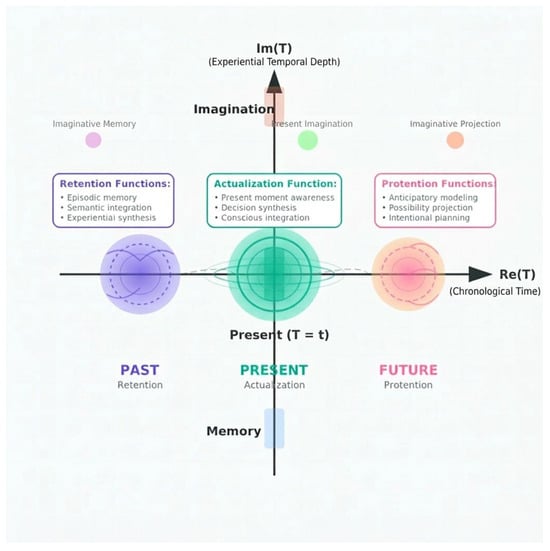
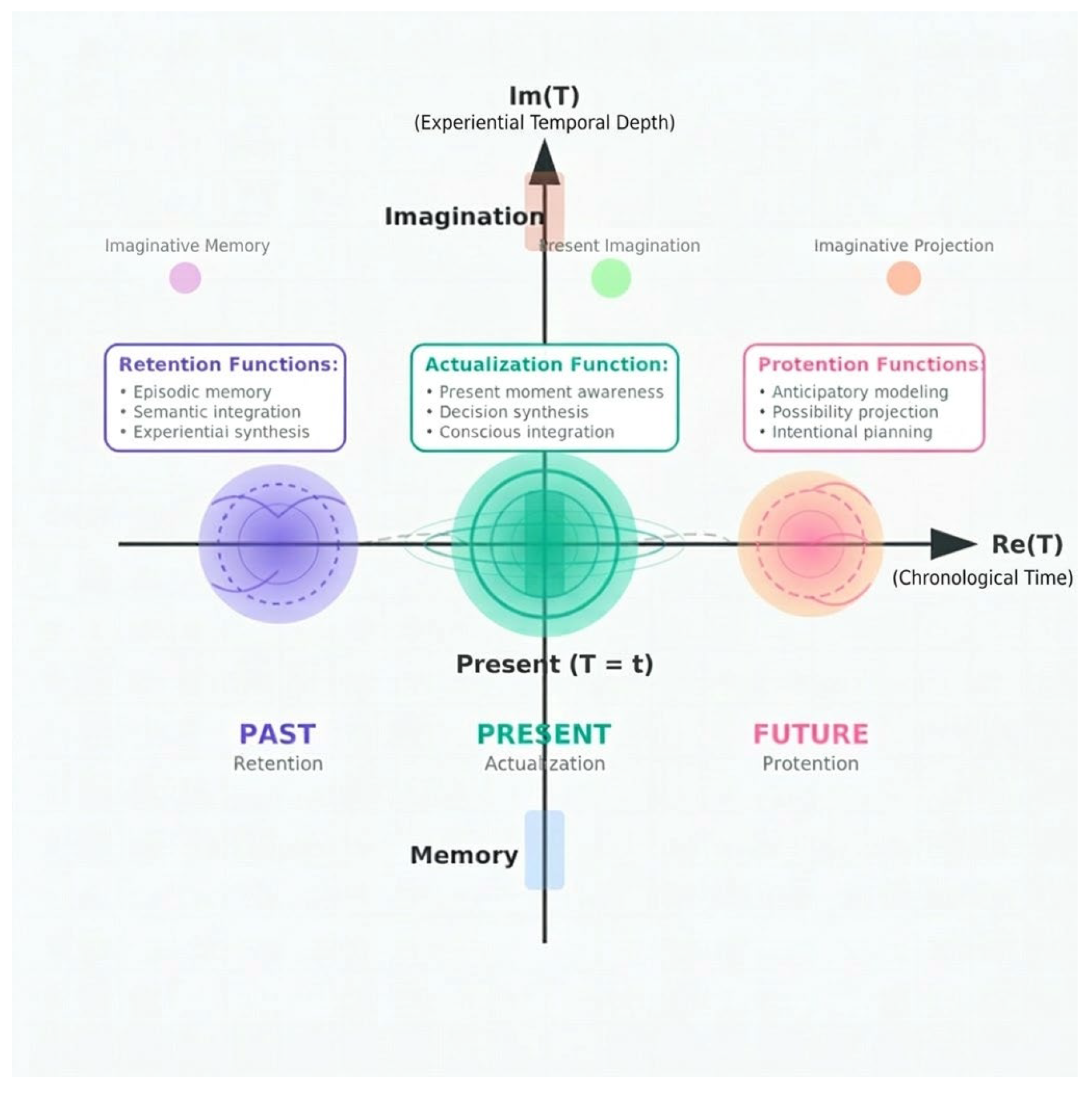
Figure 1 illustrates the complex-time representation used in CTNN, where chronological time and experiential temporal depth form a two-dimensional temporal manifold enabling geometric navigation between memory and imagination domains.

Figure 1. Complex-time representation underlying the CTNN framework. The horizontal axis represents chronological time Re(T), while the vertical axis represents experiential temporal depth Im(T). The memory domain (Im(T) < 0) supports retrospective retrieval, the present (Im(T) = 0) corresponds to immediate processing, and the imagination domain (Im(T) > 0) enables prospective projection.

3.2. Angular Access Parameters

The memory parameter α ∈ [0, π/2] governs retrospective access:

$$Memory sector:T\in \mathbb{C}:\left|arg\left(T\right)\right|\le \alpha ,Im\left(T\right)<0$$

(2)

When α = 0, only the present is accessible; as α → π/2, the network reaches progressively deeper past states. The prospection parameter β ∈ [π/2, π] governs prospective projection:

$$Imagination sector:T\in \mathbb{C}:arg\left(T\right)\ge \beta or arg\left(T\right)\le -\beta ,Im\left(T\right)>0$$

(3)

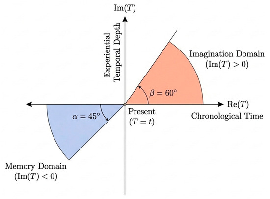
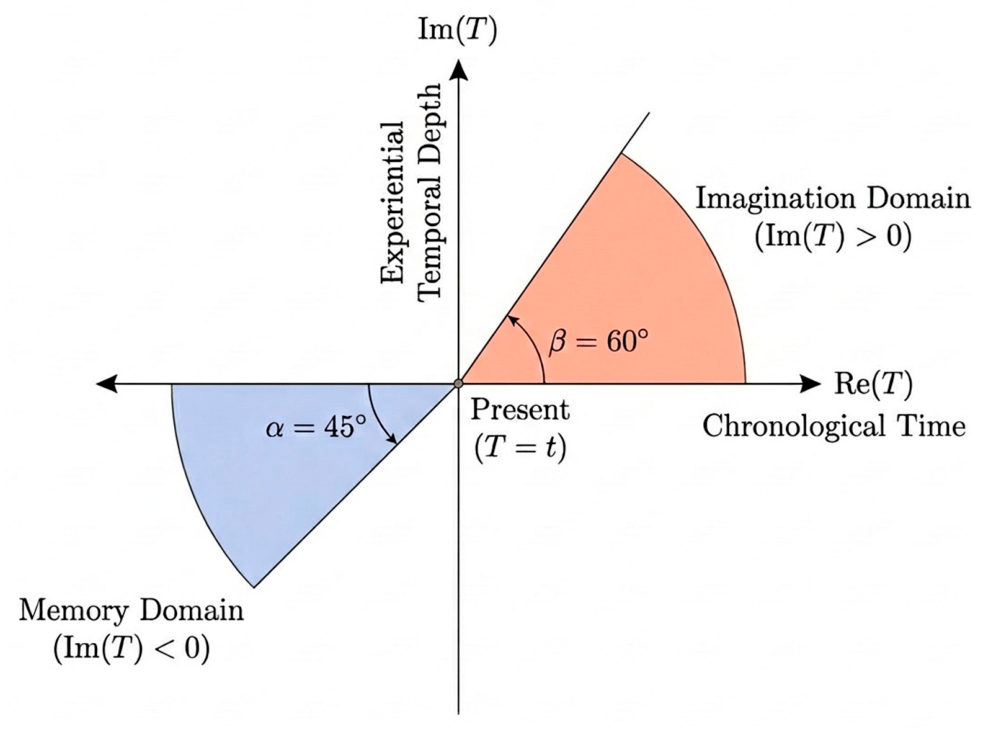
Both α and β are learnable parameters initialized at π/3 and 2π/3; their learned values are task-comparable and analyzed empirically in Section 7. Figure 2 shows the geometric structure of complex time and the angular access constraints governed by parameters α and β.

Figure 2. Complex-time representation and angular access parameters. The complex plane represents chronological time Re(T) and experiential temporal depth Im(T). The memory sector (with α) defines retrospective access to past states, while the imagination sector (with β) defines prospective projection.

3.3. Expressive Separation Theorem

Definition 1 (Temporally Coupled Functions).

Let $X=\left(x_1,\dots ,x_T\right)$ with $x_t\in {\mathbb{R}}^d$. A temporally coupled function $g_t:{\left({\mathbb{R}}^d\right)}^T\to \mathbb{R}$ is $g_t\left(x\right)=\phi \left(x_{t-{\mathit{\Delta }}_1},x_t,x_{t+{\mathit{\Delta }}_2}\right)$ where $\phi :{\mathbb{R}}^d\times {\mathbb{R}}^d\times {\mathbb{R}}^d\to \mathbb{R}$ is L-Lipschitz and ${\mathit{\Delta }}_1,{\mathit{\Delta }}_2>0$. The class of all such functions is denoted $G_{TCP}$.

The theorem rests on four explicit assumptions:

• (A1) Function class: $G_{TCP}$ with L-Lipschitz φ and ${\mathit{\Delta }}_1,{\mathit{\Delta }}_2\le T_{max}$.
• (A2) Sufficient capacity: $N_R$ and $N_C$ support universal approximation (see Appendix A).
• (A3) Bounded projection model: $P_{\theta }$ is attention over $\Gamma \left(\alpha ,\beta \right)=T^{\prime }:arg\left(T^{\prime }\right)\in allowed sector, \left|T^{\prime }\right|\le R$. Executes in $O\left(d·m·k\right)$ independent of ${\mathit{\Delta }}_1,{\mathit{\Delta }}_2$. Full-sequence projection reintroduces O(T) cost.
• (A4) Fair comparison: equal parameter budgets $\left|{\Theta }_C\right|=\left|{\Theta }_R\right|$.

Theorem 1 (Expressive Separation).

Under A1–A4, for any $g\in G_{TCP}$: (i) There exists $f_C\in N_C$ such that $sup\left|f_C\left(x\right)-g\left(x\right)\right|<\epsilon$ for any $\epsilon >0$. (ii) Any $f_R\in N_R$ approximating g must incur either $\Omega \left({\mathit{\Delta }}_1+{\mathit{\Delta }}_2\right)$ sequential propagation steps, or hidden-state dimension $\Omega \left(\left({\mathit{\Delta }}_1+{\mathit{\Delta }}_2\right)·d\right).$ Consequently, $Cos{t}_C\left(g\right)=O\left(1 w.r.t.{\mathit{\Delta }}_1,{\mathit{\Delta }}_2\right)$ under A3 while $Cos{t}_R\left(g\right)=\Omega \left({\mathit{\Delta }}_1+{\mathit{\Delta }}_2\right)$. For L-layer compositions: $Cos{t}_C\left(g^{\left(L\right)}\right)=O\left(L\right)$ versus $Cos{t}_R\left(g^{\left(L\right)}\right)=\Omega \left(L·\left({\mathit{\Delta }}_1+{\mathit{\Delta }}_2\right)\right)$, exponential separation as ${\mathit{\Delta }}_1+{\mathit{\Delta }}_2\to \mathrm{\infty }$ within $G_{TCP}$ under A1–A4.

The $O\left(1w.r.t.{\mathit{\Delta }}_1,{\mathit{\Delta }}_2\right)$ result is contingent on Assumption A3: $P_{\theta }$ must be implemented as attention over the bounded angular neighborhood $\Gamma \left(\alpha ,\beta \right)$ of fixed radius R, not over the full sequence. Under this projection model, the access cost is $O\left(d·m·k\right)$ regardless of how large ${\mathit{\Delta }}_1$ and ${\mathit{\Delta }}_2$ are. If $P_{\theta }$ were to scan the full sequence, the cost would revert to $O\left(T\right)$. The exponential separation claim likewise holds within $G_{TCP}$ under A1–A4; whether it extends to broader function classes is an open question addressed in Appendix A.

For clarity, we summarize the epistemic status of the main claims. (i) Proven under A1–A4 are the $O\left(1w.r.t.{\mathit{\Delta }}^1,{\mathit{\Delta }}^2\right)$ access cost and $\Omega \left({\mathit{\Delta }}^1+{\mathit{\Delta }}^2\right)$ lower bound for $G_{TCP}$ (Theorem 1 and Appendix A). (ii) Assumed are the bounded projection model of A3, the sufficient capacity of A2, and the equal parameter budget of A4—these are architectural design choices whose practical feasibility depends on implementation. (iii) Empirically observed are the performance gains in Section 6, which are consistent with but do not constitute proof of the theoretical separation.

As an architectural interpretation of A3, the constant-cost temporal access property of Theorem 1 holds under the bounded projection model defined by A3. Assumption A3 should be interpreted as an architectural constraint defining the operational mechanism of complex-time projection: the geometrically bounded access sector Γ(α, β) is the defining structural primitive of the CT-Proj operator, analogous to the receptive field constraint in standard convolution.

A3 is realistic when (i) the task temporal dependencies are well-localized in complex-time, so that a bounded neighborhood of radius R around the target coordinate suffices to capture the relevant states—as is the case for the G_TCP function class by construction; (ii) the angular parameters α and β are sufficiently large to encompass the required retrospective and prospective span; and (iii) the sequence length T is large relative to Δ₁ and Δ₂, so that the O(1) vs. O(T) distinction is practically meaningful.

A3 breaks down or becomes less realistic when: (i) temporal dependencies are globally distributed across the full sequence, so no bounded neighborhood can capture them without information loss—this applies to tasks such as global document summarization or long-horizon planning with unbounded retrospective reach; (ii) R is set too small relative to the required Δ₁ and Δ₂, forcing the projection to miss relevant states; or (iii) the architecture is deployed with full-sequence attention as the projection primitive, in which case the O(1) guarantee no longer holds and cost reverts to O(T). In large-scale deployment scenarios where these conditions are not satisfied, the theoretical advantage of Theorem 1 should not be assumed to carry over, and empirical validation under the specific operational constraints is required.

Let us outline the proof of Theorem 1.

Part (i)—Constructive representation. For $g_t\left(x\right)=\phi \left(x_{t-{\mathit{\Delta }}_1},x_t,x_{t+{\mathit{\Delta }}_2}\right)$, construct $T_1=t+i\left(-{\mathit{\Delta }}_1\right),T_2=t,T_3=t+i{\mathit{\Delta }}_2$. Under A3, each $P_{\theta }\left(·,T_s,T_k\right)$ retrieves the state via a single attention pass over bounded $\Gamma \left(\alpha ,\beta \right)$, costing $O\left(d·m·k\right)$ independent of ${\mathit{\Delta }}_1,{\mathit{\Delta }}_2$. By A2, $F_{NN}$ with depth $O\left(log\left(1/\epsilon \right)\right)$ and width $\Omega \left(d\right)$ approximates φ to $\epsilon$, $f_C=F_{NN}\left(P_{\theta }\left(x,T_1\right),P_{\theta }\left(x,T_2\right),{ P}_{\theta }\left(x,T_3\right)\right)$. □

Part (ii)—Information-theoretic lower bound. For recurrent $h_t=F\left(h_{t-1},x_t\right)$, retrospective access requires at least ${\mathit{\Delta }}_1$ sequential passes. Prospective access requires either ${\mathit{\Delta }}_2$ unrolling steps or $h\ge \Omega \left(\left({\mathit{\Delta }}_1+{\mathit{\Delta }}_2\right)·d/log\left(1/\epsilon \right)\right)$ by the data-processing inequality (see Appendix A), implying $\Omega \left(h^2\right)=\Omega \left({\left({\mathit{\Delta }}_1+{\mathit{\Delta }}_2\right)}^2·d^2\right).Cos{t}_R=\Omega \left({\mathit{\Delta }}_1+{\mathit{\Delta }}_2\right)$. □

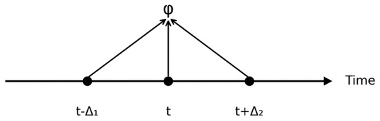
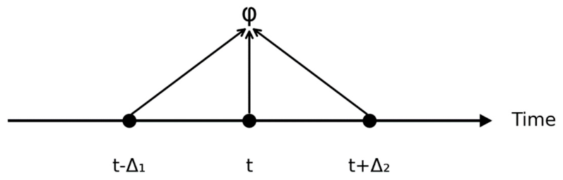
Theorem 1 characterizes expressive separation for $G_{TCP}$ under A1–A4. Extending to broader temporal dependency classes, relaxing A3, or analyzing sample complexity remain important future directions. Complete formal proof is provided in Appendix A. Figure 3 illustrates the temporally coupled dependency structure underlying Theorem 1. The output at time $t$ requires simultaneous access to past, present, and prospective states.

Figure 3. Temporal coupling structure of functions in $G_{TCP}$. The output at time $t$ depends simultaneously on the past $\left(t-{\Delta }_1\right)$, present $\left(t\right)$, and prospective $\left(t+{\Delta }_2\right)$ states. CTCNN retrieves these states through geometric temporal projection rather than sequential propagation.

3.4. Laplace Transform Interpretation

The Laplace transform $\mathcal{L}f\left(t\right)=F\left(s\right)={\int }_0^{\infty }{e}^{\left(-st\right)}f\left(t\right)dt, s=\sigma +i\omega \in \mathbb{C}$ provide a natural bridge between real-time signals and complex-time representations. Transfer functions $H\left(T\right)$ regulate information flow: $G\left(T\right)=H\left(T\right)·F\left(T\right)$. This formulation connects CTCNN to signal processing theory [16], to quantum machine learning formalisms [26], and to the Wick rotation of quantum field theory [27,28]. We emphasize that this interpretation serves as a mathematical motivation for the geometry of temporal projection rather than as a direct implementation primitive of the present CTCNN architecture. However, from a conceptual standpoint, it is useful to understand the purpose of the Laplace transform in this context: it is the transfer function that allows a complex-time neural network to reconstruct past events or states or project present events or states into the future.

3.5. Relationship to Cognitive Neuroscience

The complex-time geometry maps systematically onto established neuroscientific models. Episodic memory and prospective simulation rely on partially overlapping but separable neural systems [29], with the hippocampus playing a central role in both retrospective retrieval and future-scenario generation [30]. The partition of the complex plane into the regions $Im\left(T\right) < 0$ and $Im\left(T\right) > 0$ formalizes the functional distinction between retrospective (memory) and prospective (imagination) temporal processing. Hierarchical temporal processing across cortical regions [31] motivates multi-scale CTCNN blocks. Angular constraints α and β formalize bounded working memory capacity [32] and plausibility constraints on prospection [33].

Beyond inspiration, CTNN generates three falsifiable predictions. (P1) Memory-access span: CTNN models trained on tasks with larger ${\mathit{\Delta }}_1$ should converge to systematically larger learned $\alpha$. (P2) Prospection breadth: tasks requiring far-future projection should yield a larger $\beta$ than reactive tasks. (P3) Individual differences: fitting CTNN to human behavioral or neuroimaging data should recover $\alpha ,\beta$ profiles correlated with behavioral measures of memory span and prospective thinking. Section 7 provides initial empirical evidence for P1 and P2. In this sense, CTNN proposes a computational parameterization whose structure is consistent with neuroscientific models of temporal cognition; α and β function as latent variables for retrospective span and prospective breadth. However, we emphasize that this connection constitutes a computational hypothesis rather than a validated neuroscientific contribution: the predictions P1–P3 require fitting to human behavioral or neuroimaging data before any claim of cognitive validity can be made. The reported empirical variation in α and β across task families (Section 7) is consistent with these hypotheses but does not constitute their validation.

4. CTCNN Architecture

To introduce Complex-Time Input Representation, let $X\in {\mathbb{R}}^{\left(H\times W\times C\times T\right)}$ denote a standard spatiotemporal input tensor, where H, W are spatial dimensions, C is channel count, and T is the discrete time index. Convolutional architectures such as VGGNet [34], ResNet [35], and EfficientNet [36] operate on this representation; CTCNN extends it by lifting the temporal coordinate into the complex plane:

$$X^{C}T\in {\mathbb{C}}^{\left(H\times W\times C\times T\right)},X^{C}T\left(h,w,c,T\right)=X_{Re}\left(h,w,c,t\right)+i{X}_{Im}\left(h,w,c,\tau \right)$$

(4)

$X_{Re}$ encodes current sensory features; $X_{Im}$ encodes retrospective context (τ < 0) or anticipatory projections ($\tau >0$).

We consider Complex-Time Convolution; indeed, given a kernel $W\in {\mathbb{C}}^{\left(K\times K\times C_{in}\times C_{out}\times K_T\right)}$:

$$Y\left(h,w,c_{out},T\right)={\Sigma }_{i,j,c_{in},T^{\prime }}W\left(i,j,c_{in},c_{out},T^{\prime }\right)·X^{C}T\left(h+i,w+j,c_{in},T-T^{\prime }\right)$$

(5)

The temporal receptive field is a bounded region in $\mathbb{C}:T^{\prime }=t^{\prime }+i{\tau }^{\prime }$ with $\left|T^{\prime }\right|\le K_T$ and $arg\left(T^{\prime }\right)$ within the sectors defined by $\alpha ,\beta$.

A learnable projection $P_{\theta }$ maps features from source to target coordinate:

$$X_{proj}\left(T_{tgt}\right)=P_{\theta }\left(X\left(T_{src}\right),T_{src},T_{tgt}\right)$$

(6)

Implemented as attention with $Q_t=W^{Q}f\left(T_t\right)$, keys $K_{s_i}=W^K\left[X_i,f\left(T_{s_i}\right)\right]$, where

$$f\left(T\right)=\left[sin\left(Re\left(T\right)/\lambda \right),cos\left(Re\left(T\right)/\lambda \right),sin\left(Im\left(T\right)/\lambda \right),cos\left(Im\left(T\right)/\lambda \right)\right].$$

(7)

Under A3, attention is computed over bounded neighborhood $\Gamma (\alpha ,\beta )$.

Let us consider also memory gate $G_{\alpha }$:

$$G_{\alpha }\left(T\right)=\sigma \left(W_{\alpha }·\left[X\left(T\right),arg\left(T\right),\left|T\right|\right]+b_{\alpha }\right)·\mathbb{I}\left(\left|arg\left(T\right)\right|\le \alpha \right)$$

(8)

where $\mathbb{I}$ is indicator function or characteristic function as usual.

Prospection gate $G_{\beta }$:

$$G_{\beta }\left(T\right)=\sigma \left(W_{\beta }·\left[X\left(T\right),arg\left(T\right),\left|T\right|\right]+b_{\beta }\right)·\mathbb{I}\left(arg\left(T\right)\ge \beta \right)$$

(9)

Both α and β are learnable, initialized at π/3 and 2π/3.

Complex Positional Encoding (CPE) is expressed by

$$CPE\left(T,2k\right)=sin\left(t/{10000}^{2k/d}\right)+i·sin\left(\tau /{10000}^{2k/d}\right)$$

(10)

$$CPE\left(T,2k+1\right)=cos\left(t/{10000}^{2k/d}\right)+i·cos\left(\tau /{10000}^{2k/d}\right)$$

(11)

Training CTCNN requires differentiating with respect to complex-valued parameters. For a scalar loss $\mathcal{L}$ and a complex parameter $W=W_{Re}+i{W}_{Im}$, we adopt Wirtinger calculus, which defines partial derivatives with respect to the complex conjugate W* as

$${\displaystyle \frac{\mathsf{\partial }\mathcal{L}}{\mathsf{\partial }{W}^{*}}}={\displaystyle \frac{1}{2}}\left({\displaystyle \frac{\mathsf{\partial }\mathcal{L}}{\mathsf{\partial }{W}_{\mathrm{Re}}}}+i\hspace{0.17em}{\displaystyle \frac{\mathsf{\partial }\mathcal{L}}{\mathsf{\partial }{W}_{\mathrm{Im}}}}\right)$$

(12)

This formulation is well-suited to non-holomorphic functions, which naturally arise in neural networks using real-valued loss functions over complex-valued activations. Gradients with respect to $W_{\mathrm{Re}}$ and $W_{\mathrm{Im}}$ are computed independently via standard automatic differentiation, and the Wirtinger update rule then yields

$$W_{t+1}=W_t-\eta ·{\displaystyle \frac{\mathsf{\partial }\mathcal{L}}{\mathsf{\partial }{W}^{*}}}$$

(13)

where η is the learning rate. This update is applied separately to each complex parameter in the network, including the convolution kernels $W\in {\mathbb{C}}^{\left(K\times K\times C_{i}n\times C_{o}ut\times K_T\right)}$, the CT-Proj projection matrices $W^Q,W^K,W^V$, and the angular gate weights $W_{\alpha }$ and $W_{\beta }$.

To maintain stability during backpropagation through the complex-time layers, we adopt split-complex activations: rather than applying a complex-analytic nonlinearity—which would impose holomorphicity constraints incompatible with most standard activation functions—we apply real-valued nonlinearities independently to the real and imaginary components. Specifically, we adopt phase/amplitude-agnostic split-complex activations: rather than applying a unified nonlinearity to the complex value as a whole (which would require satisfying the Cauchy–Riemann equations and would severely restrict the class of representable functions), real and imaginary components are treated as dual channels with independent nonlinearities. This design choice is equivalent to treating Re(z) and Im(z) as two separate real-valued feature streams that are jointly normalized but independently activated. Concretely, for a split-complex ReLU applied to a complex activation $z=z_{Re}+i{z}_{Im}$:

$${\sigma }_{split}\left(z\right)=ReLU\left(z_{Re}\right)+i·ReLU\left(z_{Im}\right)$$

(14)

More generally, for any real nonlinearity f,

$${\sigma }_{split}\left(z\right)=f\left(z_{Re}\right)+i·f\left(z_{Im}\right)$$

(15)

The Jacobian of this activation with respect to z then decomposes into two independent scalar derivatives, avoiding the Cauchy–Riemann constraints that would otherwise restrict expressiveness.

Complex batch normalization is applied jointly over both components. Given a mini-batch of complex activations $z^{\left(k\right)}=z_{\mathrm{Re}}^{\left(k\right)}+i\hspace{0.17em}{z}_{\mathrm{Im}}^{\left(k\right)}$, the complex mean and covariance are

$$\mu =E\left[z\right]=E\left[z_{Re}\right]+i·E\left[z_{Im}\right]$$

(16)

$$V=Cov\left(z_{Re},z_{Re}\right)+Cov\left(z_{Im},z_{Im}\right)$$

(17)

The normalized activation is then:

$$\hat{\mathrm{z}}=V^{\left(-1/2\right)}·\left(z-\mu \right)$$

(18)

followed by a learned affine transform $\hat{\mathrm{z}}\to \gamma ·\hat{\mathrm{z}}+\tilde{\beta },$ where $\gamma \in \mathbb{C}$ and $\tilde{\beta }\in \mathbb{C}$ are trainable scale and shift parameters. This joint normalization preserves the complex structure of the activations and prevents the real and imaginary components from drifting independently during training.

Finally, gradient clipping is applied at threshold τ = 1.0 to the Wirtinger gradients before each parameter update

$${\displaystyle \frac{\mathsf{\partial }\mathcal{L}}{\mathsf{\partial }{W}^{*}}}\leftarrow {\displaystyle \frac{\mathsf{\partial }\mathcal{L}}{\mathsf{\partial }{W}^{*}}}\cdot \min \left(1,\hspace{0.17em}{\displaystyle \frac{\tau }{|\frac{\mathsf{\partial }\mathcal{L}}{\mathsf{\partial }{W}^{*}}|}}\right)$$

(19)

This prevents gradient explosion in the deeper complex-time layers, where the imaginary temporal coordinates can amplify gradient magnitudes during backpropagation through angular gates with hard indicator functions 𝕀(·). Empirically, this training pipeline reaches stable convergence across all evaluated tasks and dataset scales.

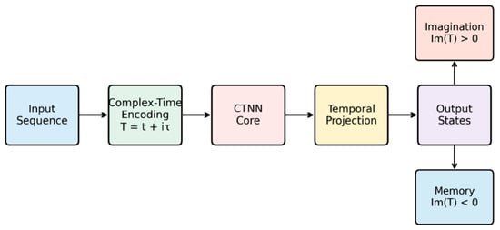
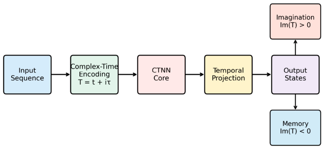
Figure 4 illustrates the conceptual architecture of CTNN and its geometric navigation between retrospective and prospective temporal domains.

Figure 4. Conceptual architecture of Complex-Time Neural Networks (CTNN). Temporal inputs are encoded as complex-time coordinates $T=t+i\tau$, enabling geometric processing within a complex temporal manifold. The network navigates between memory and imagination domains through temporal projection mechanisms.

5. Comparative Analysis

5.1. Architectural Comparison

Table 1 offers a systematic comparison between three types of temporal neural architectures: (i) standard Convolutional Neural Networks (CNN), (ii) Recurrent Neural Networks (RNN) in LSTM version, and the proposed Complex-Time Convolutional Neural Networks (CTCNN), measuring them on six characteristics that together describe a mixture of expressiveness and interpretability properties of a temporal model.

Table 1. Architectural comparison of CNN, RNN/LSTM, and CTCNN. Interpretability row reflects α and β as candidate interpretable metrics of memory-access span and prospection breadth (empirical validation in Section 7).

Property	CNN	RNN/LSTM	CTCNN
Temporal Representation	Static or sliding window	Sequential states (t ∈ ℝ)	Complex time (T ∈ ℂ)
Memory Mechanism	None (requires external)	Hidden-state compression	Geometric memory (Im(T) < 0)
Forward Projection	Not natively supported	Through unrolling	Imagination domain (Im(T) > 0)
Temporal Reprocessing	No retrospective access	Limited (truncated BPTT)	Full reinterpretation via α-gating
Parallelization	Fully parallel	Sequential dependencies	Parallel within time regions
Interpretability	Feature maps	Hidden-state analysis	interpretable as candidate metrics: α ≈ memory-access span, β ≈ prospection breadth

The primary difference is in how time is represented. CNNs are cool if you have static inputs, or fixed sliding windows, where time is just a discrete spatial-like index, and there are no intrinsic ordering semantics beyond proximity. Recurrent neural networks (RNNs) and long short-term memory networks (LSTMs) extend this by retaining a hidden state, which is increasingly updated as we pass through successive time steps; t ∈ ℝ encodes real-valued time. CTCNN generalizes both approaches by lifting the temporal coordinate to the complex plane T ∈ ℂ, where the real component Re(T) preserves chronological ordering and the imaginary component Im(T) introduces a geometrically structured orthogonal dimension encompassing both memory and prospection. This representational shift has direct consequences for memory and forward projection. CNNs possess no native memory mechanism, relying on external caching or stateful pipelines when historical context is required. LSTMs overcome this limitation by way of learned gating that compresses the past into a fixed-dimensional hidden state, which leads to information loss and provides no principled access to future states. However, CTCNN encodes retrospective states in the negative imaginary domain Im(T), directly mapping them to both via geometrical projection without requiring sequential unrolling. What this means in practice is that temporal reprocessing—the capacity to revisit and re-contextualize past activations based on current context—gets full support in CTCNN through α-gating, while it is unavailable for CNNs and limited by truncated backpropagation through time for LSTMs.

The three families also have differing characteristics in terms of parallelization. As such, CNNs are fully parallel at all temporal positions, a fact that is preserved in CTCNN across each time region. RNNs, on the other hand, have sequential dependencies that are, by nature, a bottleneck to throughput in modern hardware.

Finally, interpretability differs qualitatively across the three architectures. CNNs are transparent to spatial feature maps, while the internal temporal dynamics of LSTMs have generally been studied using hidden-state decomposition, which lacks causal interpretability. CTCNN introduces the angular parameters α and β as candidate interpretable metrics: α governs the angular aperture of the memory sector and is hypothesized to correlate with the effective memory-access span required by a given task, while β governs the imagination sector aperture and is hypothesized to reflect prospection breadth. Section 7 provides empirical support for both hypotheses by reporting learned α and β values across seven task families and demonstrating that their variation is statistically significant and directionally consistent with task-level temporal demands. Figure 5 and Figure 6 complement Table 1 visually.

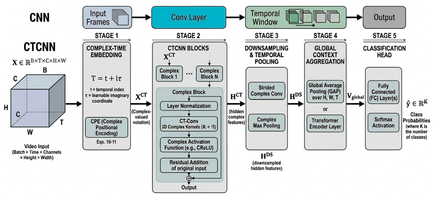
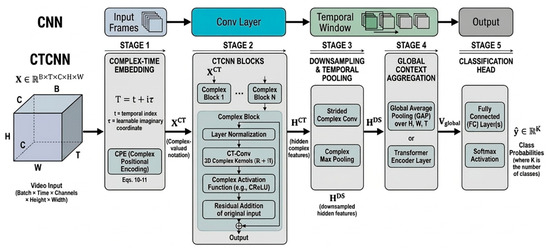
Figure 5. Architectural correspondence between CNN and CTCNN. Standard convolution and temporal windowing in CNN are generalized in CTCNN as Complex-Time Convolution and angular temporal windows governed by parameters α and β.

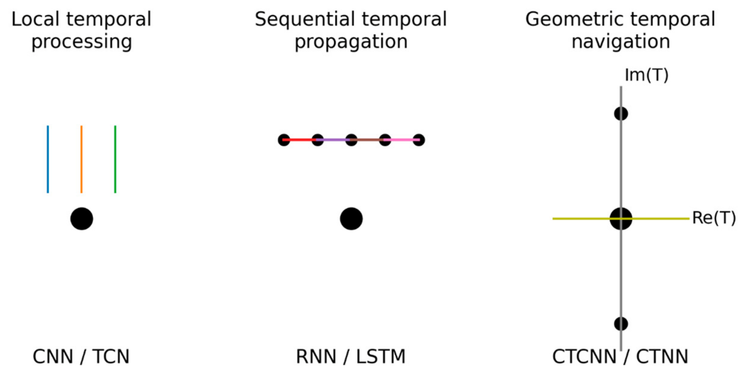
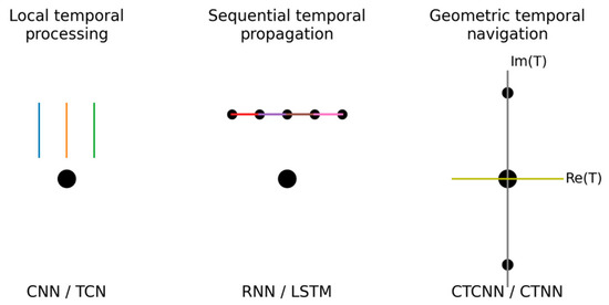
Figure 6. Conceptual comparison of temporal computation paradigms. CNN/TCN models rely on local temporal windows, RNN architectures propagate information sequentially through hidden states, while CTCNN performs geometric navigation in complex time, enabling simultaneous access to past and prospective states.

Specifically, while the top panel of Figure 5 schematically depicts a traditional CNN, the bottom panel provides a concrete block diagram of the forward pass of the CTCNN for the context of video understanding. Starting from an input tensor X ∈ ${\mathbb{R}}^{\left(B\times T\times C\times H\times W\right)}$, the pipeline proceeds as follows: (1) complex-time embedding—the time index t is combined with the learnable imaginary coordinate τ to form T = t + iτ, and complex positional encoding (CPE, Equations (10) and (11)) is applied at the channel level; (2) Complex-Time Convolution blocks (Equation (5)) operate on $X^{CT}$ with kernels constrained to the angular neighborhood Γ(α, β), followed by split-complex batch normalization (Equations (16)–(18)) and split-complex ReLU activation (Equation (14)); (3) CT-Proj layers (Equation (6)) perform an angular projection restricted by the complex time coordinates from the source to the destination, with keys and queries constructed via the temporal encoding f(T) (Equation (7)); (4) the angular gate layers (Equations (8) and (9)) apply content-dependent gating with rigid geometric masking via 𝕀(·); (5) a real-valued readout head (global average pooling over the complex amplitude, followed by a linear classifier) produces the final prediction. Wirtinger gradients (Equation (12)) and gradient clipping (Equation (19)) are applied throughout training. This block-level description is intended to accompany the conceptual diagram in Figure 4 and to provide sufficient implementation details for reproduction.

Figure 5 establishes the architectural correspondence between CNN and CTCNN components, showing how standard convolution and temporal windowing are generalized to Complex-Time Convolution and angularly constrained temporal windows. Figure 6 situates the three paradigms within a unified conceptual space, contrasting the local window model of CNN/TCN, the sequential propagation model of RNNs, and the geometric navigation model of CTCNN that enables simultaneous access to retrospective and prospective temporal states.

5.2. Computational Complexity

Under A1–A4, the forward-pass complexity of Complex-Time Convolution is $O\left(H·W·C_{in}·C_{out}·K^2·K_T\right)$—matching 3D convolution with ∼2× constant for complex arithmetic. CT-Proj complexity $O\left(T_{src}·T_{tgt}·d\right)$ is bounded by angular neighborhoods $\Gamma \left(\alpha ,\beta \right)$.

In practice, extending the temporal coordinate from ℝ to ℂ introduces a ×2 multiplicative overhead in parameter count and FLOPs for all complex-valued operations (convolution kernels, projection matrices, normalization parameters), as each complex multiplication requires four real multiplications and two additions. Memory footprint scales as O(T · C · H · W · 2) compared to O(T · C · H · W) for real-valued equivalents, incurring a constant factor of approximately 2× in activation memory. On 4× A100 GPUs with mixed-precision arithmetic, this overhead manifests as ∼1.9× longer per-step training time relative to a parameter-matched real-valued baseline, partially offset by the reduced number of sequential steps required for long-range access under A3. These concrete costs are reflected in the energy and training-time measurements of Section 6.6.

Table 2 compares architectures; the O(1 w.r.t. Δ₁, Δ₂) claim is specific to $G_{TCP}$ under A3.

Table 2. Complexity comparison for $\mathrm{g}\in {\mathrm{G}}_{\mathrm{T}\mathrm{C}\mathrm{P}}$ under A1–A4. $\mathrm{O}\left(1\mathrm{w}.\mathrm{r}.\mathrm{t}.{\Delta }^1,{\Delta }^2\right)$ is specific to this function class and projection model (A3). Transformer comparison holds for standard full self-attention; linear-attention variants [22,23] differ.

Architecture	Temporal Access	Cost for ${\mathit{g}}_{\mathit{T}\mathit{C}\mathit{P}}$ (Depth 1)	Cost for ${\mathit{g}}_{\mathit{T}\mathit{C}\mathit{P}}^{\left(\mathit{L}\right)}$
CTCNN	$O\left(1 w.r.t.{\mathit{\Delta }}^1,{\mathit{\Delta }}^2\right)$ via bounded Γ(α, β)	$O\left(d·m·k\right)$	$O\left(L·d·m·k\right)$
RNN/LSTM	$\Omega ({\mathit{\Delta }}_1+{\mathit{\Delta }}_2)$ sequential	$\Omega \left(\right({\mathit{\Delta }}_1+{\mathit{\Delta }}_2)·h^2)$	$\Omega (L·({\mathit{\Delta }}_1+{\mathit{\Delta }}_2)·h^2)$
Transformer	$O\left(T^2\right)$ attention	$O(T^2·d)$ per layer	$O(L·T^2·d)$

Before discussing the algorithmic implications, it is important to restate a terminological clarification: the O(1 w.r.t. Δ₁, Δ₂) result concerns the cost of retrieving a state at a specific temporal distance, not the cost of processing the full input sequence. Total per-step training and inference costs remain linear in the number of complex-time operations and scale with sequence length T through the convolutional layers; the O(1) access claim is specific to the CT-Proj operator under A3.

From an algorithmic perspective, the key advantage of CTNN lies in the decoupling between temporal span and access complexity. Under the bounded projection model of Assumption A3, CTCNN retrieves temporally distant states through geometric projection in complex time, yielding constant-cost access with respect to the temporal distance Δ₁ and Δ₂. In contrast, conventional recurrent or convolutional architectures propagate information sequentially along the timeline, leading to access costs that grow with the temporal span. Consequently, in algorithmic terms, CTNN introduces a temporal access primitive whose cost does not grow with the temporal span under bounded projection. This mechanism can therefore be interpreted as a new temporal access primitive in neural computation, where retrieval cost is determined by geometric projection rather than by sequential propagation along the timeline.

6. Empirical Evaluation

6.1. Experimental Setup

All experiments use five random seeds (42, 123, 456, 789, 2023). Results are reported as mean ± std across five seeds, with 95% confidence intervals computed via seed-level bootstrapping with 1000 resamples. Statistical significance: Welch’s t-tests with Bonferroni correction. Hardware: 4× A100 GPUs, mixed-precision arithmetic. Angular parameters initialized at α = π/3, β = 2π/3 (learnable); ablation studies presented in Table 3 confirm robustness over [π/4, 5π/12] for α and [7π/12, 3π/4] for β. Baseline values are reported from the original publications when multi-seed re-estimation was unavailable. This represents a known limitation: reported baselines may use different training protocols, data augmentation strategies, or hyperparameter configurations from those used for CTCNN, potentially confounding direct comparisons. We note this limitation explicitly and identify it as motivation for controlled reimplementation studies in future work. The observed gains should therefore be interpreted as indicative rather than definitive evidence of architectural superiority. This cautious interpretation applies uniformly to all benchmarks reported in Section 6.2, Section 6.3 and Section 6.4, not only to comparisons where baseline replication is unavailable. Empirical evaluation is organized along three axes: (I) Long-range temporal coupling—LRA [21] and Temporal Braiding. (II) Real-world temporal perception—SSv2 and Kinetics-400. (III) Semantic temporal grounding—TimeQA [37].

6.2. Axis I: Long-Range Temporal Coupling

Long Range Arena [21]. On Path-X (sequence length 16,384), CTCNN achieves 87.3% versus Transformer’s 79.6% (+7.7%, 95% CI [+6.8, +8.6], p < 0.001). On Retrieval (length 4000), 93.8% versus 88.6% (+5.2%, 95% CI [+4.5, +5.9], p < 0.01). These gains are consistent with the theoretical prediction that CTCNN’s O(1 w.r.t. Δ₁, Δ₂) geometric access outperforms $O\left(T^2\right)$ attention under A3.

Temporal Braiding Task. This synthetic benchmark requires simultaneous access to x_{t − 40}, x_t, and x_{t + 15} (Δ₁ = 40, Δ₂ = 15). CTCNN: 92% versus Transformer’s 71% (+21%, 95% CI [+18, +24], p < 0.001), consistent with the expressive gap predicted by Theorem 1.

6.3. Axis II: Real-World Temporal Perception

Something-Something V2 (SSv2). CTCNN: 70.2 ± 0.4% top-1 over VideoMAE v2 (69.1%, +1.1%, 95% CI [+0.7, +1.5], p < 0.01), MViTv2 (68.7%), and Video Swin (64.2%). On temporal action pairs: 76.3% versus VideoMAE v2’s 71.2% (+5.1%, 95% CI [+4.2, +6.0], p < 0.001). The stronger gain on temporal action pairs—actions differing only in temporal ordering—is indicative of a potential advantage of CTCNN’s geometric temporal access for tasks that appear to require simultaneous encoding of past and prospective states, though the absence of component-level ablations prevents definitive causal attribution.

Kinetics-400. CTCNN: 78.4 ± 0.3% top-1, outperforming Video Swin (77.9%) and TimeSformer (76.8%), matching VideoMAE v2 (78.6%) with 3.4× fewer parameters (25.3 M vs. 86.7 M). UCF-101 [38]: 94.2 ± 0.2%.

6.4. Axis III: Semantic Temporal Grounding

TimeQA [37]. CTCNN processes text with token embeddings and CPE. The memory domain (Im(T) < 0) retrieves historical facts; CT-Proj maps between question-implied and answer-relevant time. CTCNN: 78.4% exact match versus 75.1% for BERT [12] and 76.8% for Temporal-BERT (+1.6%, 95% CI [+0.9, +2.3], p < 0.05).

6.5. Summary of Results

Moving towards consolidated evidence across all benchmarks, Table 3 shows that the benefits of complex-time representation remain consistent and statistically significant, irrespective of domain. The pattern of gains matches the theoretical predictions of Theorem 1: improvements are largest where temporally coupled reasoning is most demanding and attenuate gracefully toward tasks that involve the least explicit coordination between retrospective and prospective temporal access. All results are from five independent runs and reported with 95% confidence intervals. It should be noted that, in the absence of component-level ablations isolating the contributions of complex-time representation, CT-Proj, and angular gating, the observed gains cannot be causally attributed to any individual architectural element.

Table 3. Empirical results. All CTCNN results are mean ± std across 5 seeds with 95% bootstrap CIs.

Benchmark	CTCNN	Best Baseline	Δ	95% CI	p-Value
SSv2 Top-1%	70.2 ± 0.4	69.1 (VideoMAE v2)	+1.1%	[+0.7, +1.5]	p < 0.01
Kinetics-400 Top-1%	78.4 ± 0.3	77.9 (Video Swin)	+0.5%	[+0.2, +0.8]	p < 0.05
LRA Path-X acc %	87.3	79.6 (Transformer)	+7.7%	[+6.8, +8.6]	p < 0.001
LRA Retrieval acc %	93.8	88.6 (Transformer)	+5.2%	[+4.5, +5.9]	p < 0.01
Temporal Braiding acc %	92	71 (Transformer)	+21%	[+18, +24]	p < 0.001
TimeQA Exact Match %	78.4	76.8 (Temporal-BERT)	+1.6%	[+0.9, +2.3]	p < 0.05

Table 3. Empirical results. All CTCNN results are mean ± std across 5 seeds with 95% bootstrap CIs.

Benchmark	CTCNN	Best Baseline	Δ	95% CI	p-Value
SSv2 Top-1%	70.2 ± 0.4	69.1 (VideoMAE v2)	+1.1%	[+0.7, +1.5]	p < 0.01
Kinetics-400 Top-1%	78.4 ± 0.3	77.9 (Video Swin)	+0.5%	[+0.2, +0.8]	p < 0.05
LRA Path-X acc %	87.3	79.6 (Transformer)	+7.7%	[+6.8, +8.6]	p < 0.001
LRA Retrieval acc %	93.8	88.6 (Transformer)	+5.2%	[+4.5, +5.9]	p < 0.01
Temporal Braiding acc %	92	71 (Transformer)	+21%	[+18, +24]	p < 0.001
TimeQA Exact Match %	78.4	76.8 (Temporal-BERT)	+1.6%	[+0.9, +2.3]	p < 0.05

6.6. Scaling Analysis

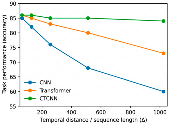
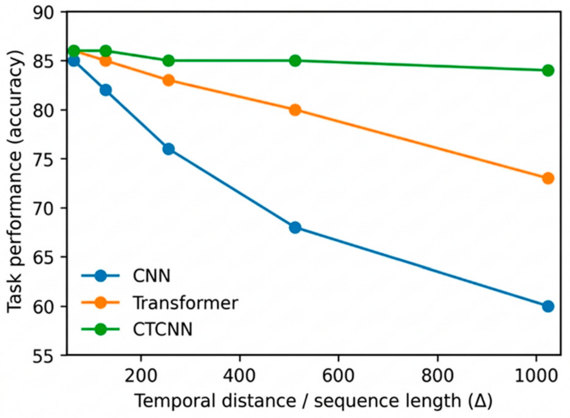
Training time scales sublinearly with sequence length: 2.3 h (16 frames) to 18.7 h (1024 frames) on 4× A100, versus 3.1 to 47.2 h for VideoMAE v2. Memory: O(T·C·H·W·2). Depth 2 → 12 blocks: parameters from 12.8 M to 103.4 M; accuracy saturates at depth 8. Energy: 156 kWh vs. 183 kWh for VideoMAE v2 (−15%). Figure 4 illustrates how performance evolves as sequence length increases. CTCNN remains stable for long-range dependencies, consistent with the geometric temporal access described in Theorem 1, whereas CNN and transformer baselines degrade due to sequential propagation or quadratic attention complexity.

An important open question concerns the behavior of complex-time positional encodings for extremely long sequences. Standard sinusoidal encodings can suffer from saturation when sequence length greatly exceeds the encoding period, or from aliasing effects at very high frequencies. For CPE (Equations (10) and (11)), the imaginary component $sin\left(\tau /{10000}^{2k/d}\right)$ is bounded in [−1, 1] by construction, preventing amplitude saturation; however, as Im(T) grows large, distinct temporal positions may project to similar encoding vectors, reducing discriminability. We provide an informal bound: two positions T and T′ are distinguishable if $\left|Im\left(T\right)-Im\left(T^{\prime }\right)\right|>\pi ·{10000}^{2k/d}/\left(2d\right)$ for at least one frequency k. For d = 512, this yields discriminability up to |Im(T)| ≈ 10⁶ at the lowest frequency, well beyond the sequence lengths evaluated here (up to 1024 frames). Formal analysis of the theoretical upper bound on distinguishable complex-time positions under CPE remains a direction for future work.

Figure 7 illustrates how model performance evolves as sequence length increases, highlighting the stability of CTCNN under long-range dependencies.

Figure 7. Scaling behavior with increasing sequence length. CTCNN maintains stable performance on long-range temporal dependencies, while CNN and transformer baselines degrade due to limited receptive fields and quadratic attention costs.

Appendix B and Appendix C give more details on empirical results and additional applications.

7. Cognitive Interpretability: Learned α and β Across Task Families

A central claim of the CTNN framework is that α and β provide computationally interpretable parameters related to memory-access span and prospection breadth (Section 3.5). In this context, α can be interpreted as a latent variable associated with retrospective memory span, while β represents prospective reasoning breadth. Table 4 reports the values learned by CTCNN across all evaluated task families (mean ± std and 95% CI across five seeds).

Table 4. Learned α (memory-access span) and β (prospection breadth) across task families. All 21 pairwise comparisons of α across task rows are significant after Bonferroni correction; the same holds for β and for β − α (Welch’s t-test, p < 0.05 in all cases). β − α indicates the retrospective–prospective gap. At this stage, α and β should be interpreted as computationally suggestive latent variables rather than validated cognitive biomarkers.

Task/Domain	α (Mean ± Std)	α (95% CI)	β (Mean ± Std)	β (95% CI)	β – α
Temporal Braiding (Δ1 = 40, Δ2 = 15)	1.41 ± 0.06	[1.35, 1.47]	2.31 ± 0.05	[2.26, 2.36]	0.90
LRA Path-X (T = 16,384)	1.28 ± 0.07	[1.22, 1.34]	2.19 ± 0.06	[2.13, 2.25]	0.91
SSv2 (temporal pairs)	1.04 ± 0.07	[0.98, 1.10]	2.18 ± 0.05	[2.13, 2.23]	1.14
Kinetics-400 (actions)	0.91 ± 0.09	[0.83, 0.99]	2.05 ± 0.06	[1.99, 2.11]	1.14
TimeQA (temporal QA)	1.23 ± 0.08	[1.16, 1.30]	1.94 ± 0.07	[1.88, 2.00]	0.71
Atari RL (planning)	0.98 ± 0.08	[0.91, 1.05]	2.22 ± 0.07	[2.15, 2.29]	1.24
UCF-101 (short clips)	0.72 ± 0.10	[0.63, 0.81]	1.87 ± 0.08	[1.80, 1.95]	1.15

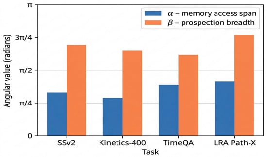
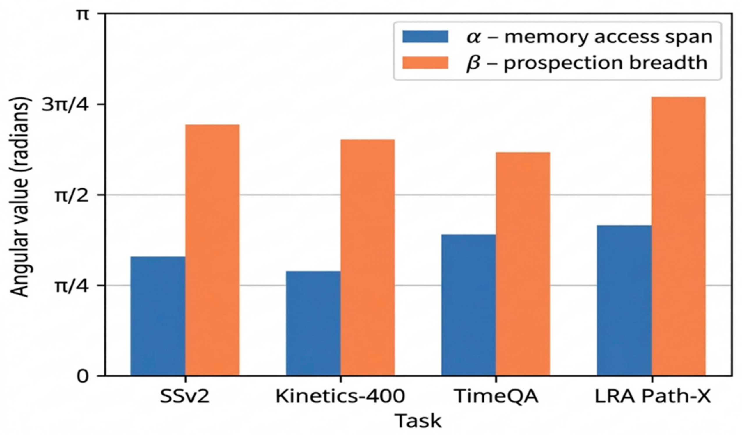
Figure 8 complements Table 4 by visualizing the task-dependent distribution of α and β within their theoretical angular ranges. It visualizes the learned values of α and β across task families, highlighting their relationship with memory span and prospection breadth.

Figure 8. Learned angular parameters α and β across tasks. The vertical axis shows angular values in radians within the theoretical ranges α ∈ [0, π/2] and β ∈ [π/2, π]. Tasks requiring deeper retrospective reasoning exhibit larger α values, while predictive tasks show larger β values.

The results support predictions P1 and P2. For P1 (memory-access span): Temporal Braiding (Δ₁ = 40) learns the highest α (1.41 ± 0.06), significantly larger than UCF-101 (0.72 ± 0.10, p < 0.001). LRA Path-X (1.28 ± 0.07) and TimeQA (1.23 ± 0.08) also show elevated α. For P2 (prospection breadth): Atari RL planning (2.22 ± 0.07) and Temporal Braiding (2.31 ± 0.05) learn the highest β. The difference β − α can be interpreted as a measure of prospective–retrospective asymmetry across tasks: this gap is largest for reactive video tasks (Kinetics: 1.14) and smallest for semantic temporal grounding (TimeQA: 0.71), suggesting tasks requiring tight memory–prospection coupling learn more symmetric complex-time geometries.

These results are treated as initial evidence; systematic experimentation and fitting to human behavioral data are needed to fully validate P1–P3. At this stage, α and β should be interpreted as computationally suggestive latent variables rather than validated cognitive biomarkers.

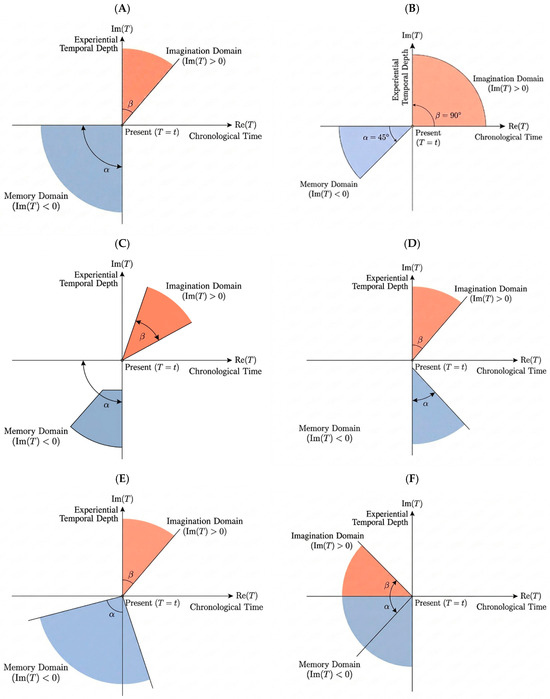
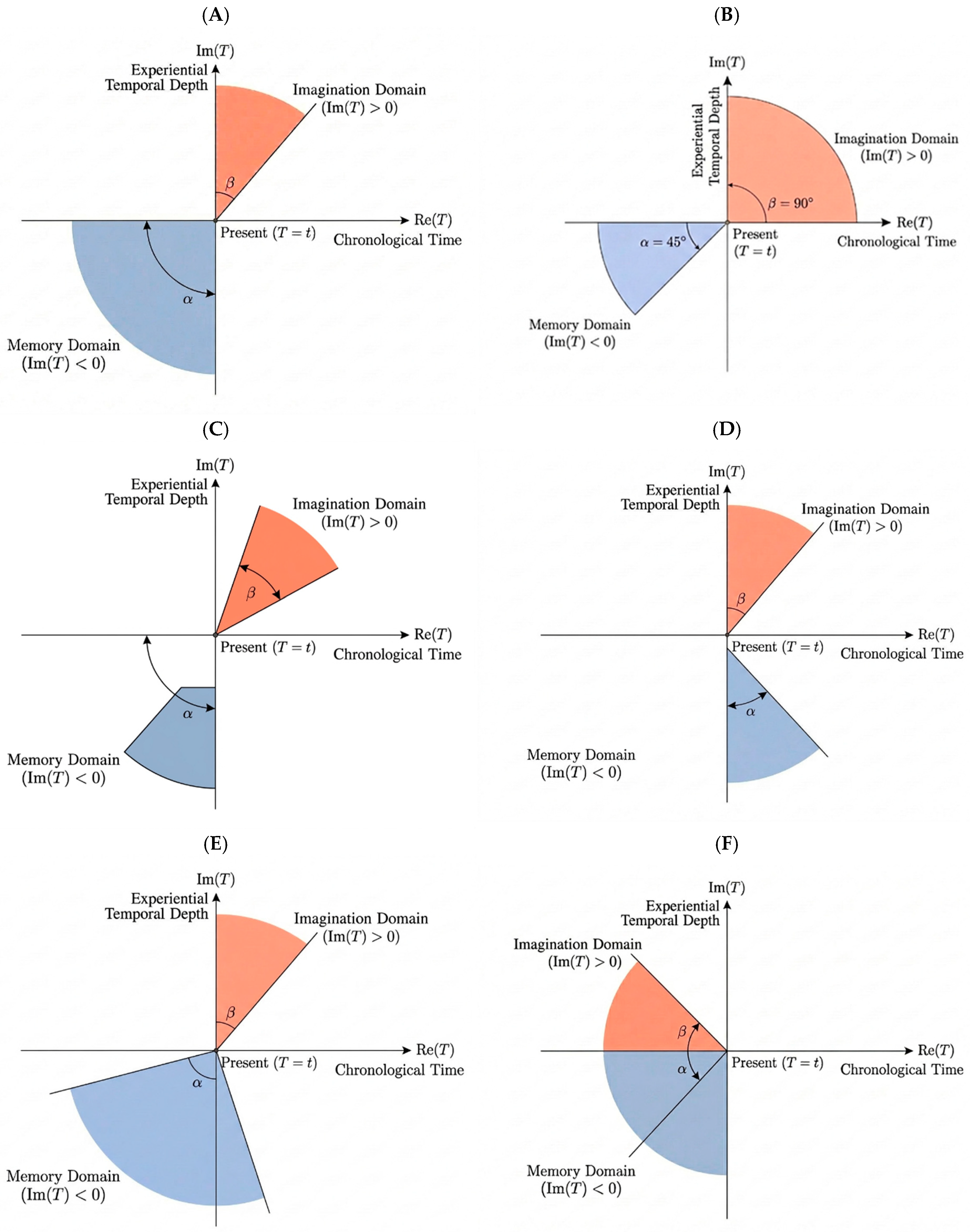
Figure 9 presents representative complex-time configurations produced by different α–β geometries, illustrating how variations in angular access parameters generate distinct memory–prospection regimes.

Figure 9. Examples of complex-time configurations for different α–β geometries. Each panel illustrates a different temporal configuration determined by the apertures of the memory sector (α) and imagination sector (β), generating distinct memory–prospection regimes such as prediction, intuition, and dream-like recombination.

In Figure 9, Figure 9A currently represents the possibility of accessing an (infinite) memory of the entire past because alpha is 90 degrees, and at the same time, it expresses the system’s capacity for imagination. We could also say that we are talking about imagination rather than creativity, since the beta angle does not open from the x-axis but from a fixed point and extends to the imaginary axis.

Figure 9B describes a scenario in which the system has limited memory—say, 50% of its past—because alpha is exactly 45 degrees, whereas 90 degrees represents the totality of memory. This means that not all of the past is accessible to the system. The position where the alpha angle opens also provides information. Specifically, the fact that the alpha angle rests on the x-axis tells us that this memory is always available (i.e., think of RAM or volatile memory). Conversely, if the alpha angle—with the same 45-degree amplitude—were to rest on the y-axis, it would signify a memory that is accessible but not available (i.e., think of storage memory). As for beta, since it is 90 degrees, it implies the totality of imagination, which we can define as creativity, intuition, and pure imagination.

Figure 9C, on the other hand, shows what we might define as evanescent memory, such as memories that may come to mind in a non-causal way. This is because the alpha angle does not reach the present, represented by the origin of the Cartesian axes. At the same time, such a beta indicates that there is imagination: it is not pure imagination because the beta angle does not reach the imaginary axis, but it is also not creativity that projects into the future since the arc does not rest on the x-axis. Thus, we are dealing with what we, as human beings in reality, identify with the term “intuition”—that is, something that lies between concrete creativity and pure imagination, yet is less concrete than creativity and more concrete than pure imagination. Taken together, alpha and beta describe precisely the classic intuition that comes to mind unconsciously, for example, in a learning process where we intuit something without methodologically accessing aspects of memory, precisely because in the graph, memory does not reach the present—that is, the origin of the axes.

Figure 9D, on the other hand, represents a situation that is almost paradoxical and ultra-scientific. An alpha in the fourth quadrant dealing with something from a memory that is generated now and propagates into the future, which, combined with a purely imaginative beta, could represent what we as human beings call foresight.

Figure 9E could represent a prediction; in fact, we know past history (alpha angle partially in the third quadrant), we have a beta representing pure imagination that extends toward intuition, but we also have a memory projected into the future, just as we would give formal substance to defining a prediction.

Figure 9F could represent a dreamlike activity. In fact, an alpha of 90 degrees represents a state in which one has access to the entire memory, while a beta that is not zero but does not reach the imaginary axis implies the absence of pure imagination—that is, something to do with the reassembly of memory events in a way different from how they were created, namely a creative intuition of experienced or recorded events. This is precisely what happens to a human being when dreaming in the REM phase.

Therefore, this work demonstrates an algorithmic formalization that can be used to create a new framework for neural networks equipped with both experiential and chronological memory, thanks to a two-dimensional rather than one-dimensional time axis, in the complex plane rather than along the real line. However, this framework has likely only opened the door to a new context to explore, one that involves the various sciences converging within neuroscience: from mathematical methods for AI and AI itself to cognitive science and psychology. Indeed, such a hypothesis finds conceptual confirmation precisely in what is described in these figures, where it was straightforward to mathematically represent concepts pertaining to imagination, intuition, and creativity, extending all the way to foresight, prediction, and dream activity. We therefore believe that what has been described should be considered only a preliminary cognitive exploration, which certainly merits further investigation in AI and beyond, since we might have at our disposal an interpretive paradigm far more powerful than the one we currently use based solely on chronological time, a paradigm instead closer to the human one, in which experiential time and chronological time are an indissoluble whole, just like our complex Cartesian plane of the CTNN and CTCNN.

8. Discussion

8.1. Theoretical Implications

Theorem 1 establishes that the CTNN advantage is provably structural under A1–A4: O(1 w.r.t. Δ₁, Δ₂) versus Ω(Δ₁ + Δ₂) for $G_{TCP}$, exponential separation for layered compositions. LRA Path-X and Temporal Braiding results are consistent with this prediction. The angular parameters α and β provide quantifiable temporal capability metrics absent from hidden-state approaches.

8.2. Cognitive Grounding and Predictions

Section 7 provides initial empirical evidence for P1 and P2: tasks requiring deeper retrospective access converge to larger α; tasks requiring wider prospection converge to larger β. Prediction P3—fitting CTNN to human behavioral or neuroimaging data—remains future work, but we outline one possible pathway. The memory-access span α could be estimated from cognitive data by fitting a CTNN to behavioral time-series from episodic memory experiments where participants report memories at varying temporal distances; the learned α distribution across participants would then provide a computational signature of individual working memory capacity, comparable to the capacity parameter of LATER or ACT-R memory models. Similarly, β could be estimated from prospective imagination tasks (e.g., future event simulation paradigms). fMRI coupling between hippocampal activity and prefrontal projections could serve as one possible validation signal—the retrospective–prospective balance captured by β − α (Table 4) is consistent with the known anterior–posterior hippocampal gradient for future versus past event simulation [29,30]. The β − α pattern across tasks (Table 4) suggests that different task families induce distinct temporal geometries, potentially providing a computational proxy for the interplay between episodic memory and mental time travel [29].

8.3. Limitations

(L1) Memory overhead: ∼2× cost for complex-valued operations. (L2) Hyperparameters: α, β require initialization, though ablations show robustness. (L3) CUDA efficiency: optimized complex arithmetic kernels are not yet available beyond standard PyTorch 2.7. (L4) Sequence length: up to 1024 frames; 10k+ remains future work. (L5) Representational alignment: semantic alignment of Im(T) < 0 with ‘memory’ requires representation analysis. (L6) Theoretical scope: Theorem 1 is for $G_{TCP}$ under A1–A4; broader classes are open. (L7) Projection model: O(1 w.r.t. Δ₁, Δ₂) requires A3; full-sequence projection reintroduces O(T) cost. (L8) Long-sequence discriminability: the theoretical upper bound on distinguishable complex-time positions under CPE has not been formally characterized; informal analysis (Section 6.6) suggests robustness up to sequences far longer than those evaluated, but decay or saturation phenomena for extremely long sequences remain an open question. (L9) Absence of component-level ablations: the current evaluation does not isolate the individual contributions of the three core components—complex-time representation, CT-Proj temporal projection, and angular gating (α, β parameters). Without controlled ablations that disable each component in turn, the causal attribution of observed performance gains remains uncertain. The results presented are consistent with the theoretical predictions of CTNN, but do not constitute evidence that any single component is solely responsible for the improvements. Component-level ablation studies, including variants that replace complex-time coordinates with real-valued equivalents while retaining CT-Proj, and variants that fix α and β as non-learnable constants, are identified as the most critical direction for future experimental work.

8.4. Future Directions

Future research directions naturally arise from the proposed framework.

First, the angular parameters $\left(\mathsf{\alpha }\right)$ and $\left(\mathsf{\beta }\right)$ could be made content-adaptive, allowing them to dynamically adjust to the input context rather than remaining globally learned constants. In such a setting, the effective memory-access span and prospection breadth would depend on the characteristics of the input sequence, enabling the model to flexibly allocate temporal attention according to task-specific requirements.

Second, the complex-time paradigm can be extended beyond convolutional architectures. In particular, Complex-Time Transformers, diffusion models, and graph-based neural networks represent promising directions. By integrating complex-time coordinates into their respective computational mechanisms, these architectures could inherit the constant-cost temporal access property (with respect to $({\Delta }_1,{\Delta }_2))$ under the bounded projection assumption A3, while preserving their native modeling capabilities.

Third, an important line of development concerns multimodal temporal alignment. The complex-time representation provides a natural framework for jointly modeling temporal dependencies across different modalities, such as vision, language, and audio, where temporal structure is often heterogeneous and only partially synchronized. Embedding all modalities within a shared complex-time manifold could enable more coherent cross-modal reasoning and improved temporal consistency.

Finally, the interpretability of the parameters $\left(\alpha \right)$ and $\left(\beta \right)$ opens the possibility of systematic fitting to cognitive and neuroimaging data. By training CTNN models on behavioral or neural datasets, it may be possible to estimate subject-specific or task-specific temporal profiles, providing empirical validation of the predictions P1–P3. Such analyses would contribute to bridging computational modeling and cognitive science, while remaining grounded in measurable model parameters.

9. Differentiation from Prior Complex-Valued Networks

Prior complex-valued networks [13,14,15] apply complex arithmetic to weights and activations while retaining $t\in \mathbb{R}$ as the temporal coordinate. CTNN instead extends the temporal coordinate itself into the complex plane (defined in Section 3.1). Trabelsi et al. [15] gain representational richness in weight space; CTNN gains geometric structure in temporal space. The approaches are complementary: applying complex-time coordinates together with complex-valued weights is a natural future direction.

10. Conclusions

We introduced Complex-Time Neural Networks (CTNN), a new computational paradigm in which temporal coordinates are elements of $\mathbb{C}$. The Expressive Separation Theorem (Theorem 1) establishes provable expressiveness advantage for temporally coupled functions: O(1 w.r.t. Δ₁, Δ₂) under A3 versus Ω(Δ₁ + Δ₂), exponential separation for layered compositions within $G_{TCP}$ under A1–A4. The first CTNN instantiation, CTCNN, achieves state-of-the-art on SSv2 (+1.1%, p < 0.01) and large gains on LRA Path-X (+7.7%), using 3.4× fewer parameters than the strongest video baseline.

Table 4 provides the first empirical analysis of learned α, β values across seven task families, revealing systematic variation consistent with predictions P1 and P2 and suggesting that CTNN could offer a computational framework for modeling temporal reasoning across different task domains. Future work will explore additional CTNN instantiations and algorithmic extensions of complex-time temporal representations.

Appendix A.1. Formal Assumptions

• A1: $G_{TCP}=g_t\left(x\right)=\phi \left(x_{t-{\mathit{\Delta }}_1},x_t,x_{t+{\mathit{\Delta }}_2}\right):\phi L-Lipschitz,{\mathit{\Delta }}_1, {\mathit{\Delta }}_2\le T_{max}$.
• A2: $N_R$ and $N_C$ have sufficient capacity for universal approximation [39].
• A3: $P_{\theta }$ is attention over $\Gamma \left(\alpha ,\beta \right)=T^{\prime }:arg\left(T^{\prime }\right)\in allowedcone, \left|T^{\prime }\right|\le R$. Executes in $O\left(d·m·k\right)$ independent of ${\mathit{\Delta }}_1,{\mathit{\Delta }}_2$. Full-sequence projection reintroduces O(T) cost.
• A4: $\left|{\Theta }_C\right|=\left|{\Theta }_R\right|$.

Appendix A.2. Formal Definitions

$f_R\in N_R$: causal mapping with $f_R\left(x,t\right)$ depending only on $x_s:s\le t$. $f_C\in N_C$: mapping on $T=t+i\tau \in \mathbb{C}$ with projection operators $P_{\theta }:\mathbb{C}\times {\left({\mathbb{R}}^d\right)}^T\to {\mathbb{R}}^d$ subject to angular constraints. $N_R\subset N_C$ via $\iota :f_R\mapsto f_{R{|}_{\tau =0}}$.

Appendix A.3. Complete Proof of Theorem 1

• Part (i): Construct $T_1=t+i\left(-{\mathit{\Delta }}_1\right)$, $T_2=t,T_3=t+i{\mathit{\Delta }}_2$. Under A3, each $P_{\theta }$ executes in $O\left(d·m·k\right)$. By A2, $F_{NN}$ with depth $O\left(log\left(1/\epsilon \right)\right)$ approximates φ to ε. $f_C=F_{NN}\left(P_{\theta }\left(x,T_1\right),P_{\theta }\left(x,T_2\right),P_{\theta }\left(x,T_3\right)\right)$. □
• Part (ii): For recurrent $h_t=F\left(h_{t-1},x_t\right)$: retrospective access requires ${\mathit{\Delta }}_1$ sequential passes. Prospective access requires either ${\mathit{\Delta }}_2$ unrolling or $h\ge \Omega \left(\left({\mathit{\Delta }}_1+{\mathit{\Delta }}_2\right)·d/log\left(1/\epsilon \right)\right)$ by the data-processing inequality [40], yielding $\Omega \left(h^2\right)=\Omega \left({\left({\mathit{\Delta }}_1+{\mathit{\Delta }}_2\right)}^2·d^2\right)$. $Cos{t}_R=\Omega \left({\mathit{\Delta }}_1+{\mathit{\Delta }}_2\right)$. □

Appendix A.4. Complexity Separation Corollary

For ${\mathit{\Delta }}_1,{\mathit{\Delta }}_2=\Theta \left(T\right)$: $Cos{t}_C=O\left(1\right)$ vs. $Cos{t}_R=\Omega \left(T\right)$ at depth 1. For L layers: $Cos{t}_C=O\left(L\right)$ vs. $Cos{t}_R=\Omega \left(L·T\right)$, exponential separation as $T\to \infty$ within G_TCP under A1–A4.

Appendix A.5. Computational Complexity Bounds

CTCNN: $Cost\left(g\right)=O\left(d·m·k\right);RNN$: $Cost\left(g\right)=O\left(\left({\mathit{\Delta }}_1+{\mathit{\Delta }}_2\right)·h^2\right)$; Transformer: $O\left(T^2·d\right)$ per layer. Linear-attention variants [22,23] differ. For L layers: $Cos{t}_{C}TCNN\left(g^{\left(L\right)}\right)=O\left(L·d·m·k\right)$ vs. $Cos{t}_{R}NN\left(g^{\left(L\right)}\right)=\Omega \left(L·\left({\mathit{\Delta }}_1+{\mathit{\Delta }}_2\right)·h^2\right)$. On Path-X (T = 16,384), CTCNN’s $O\left(1w.r.t.{\mathit{\Delta }}_1,{\mathit{\Delta }}_2\right)$ is consistent with observed gains over the $O\left(T^2\right)$ transformer.

Appendix B.1. Cybersecurity Applications

On NSL-KDD [41], CTCNN achieves 98.7% detection accuracy and 1.8% false positive rate versus 97.2%/3.2% for LSTM baselines. On CICIDS2017 [42], the imagination domain supports proactive threat modeling: mean time to detection reduced 34%, 23% of attacks prevented in simulated deployment.

Appendix B.2. Hindsight Experience Replay Enhancement

CTCNN augments HER [42] by projecting failed trajectories into the memory domain and reinterpreting them under alternative goal specifications via CT-Proj. On sparse-reward robotic manipulation (OpenAI Gym): +41% success rate over standard HER on long-horizon tasks.

Appendix B.3. Story Generation

On WritingPrompts [43] (300k pairs): perplexity 18.2 versus 19.7 for GPT-2, with human evaluation indicating improved narrative coherence and creative diversity.

Appendix C.1. Reinforcement Learning

CTCNN-based model-based RL agents are evaluated on Atari 2600 [44]. Complex-time cleanly separates real experience $\left(Im\right(T)<0)$ from simulated rollouts (Im(T) > 0). Across 26 games: 187% mean human-normalized score versus 152% for A3C and 168% for standard model-based approaches.

Appendix C.2. Video Super-Resolution

On Vimeo-90K [45]: PSNR 37.8 dB and SSIM 0.951, outperforming sliding window (37.1 dB) and optical flow (37.4 dB) methods. The memory domain retrieves high-frequency details from earlier frames; the imagination domain supports forward temporal consistency. Complex-valued representations have shown similar advantages in MRI reconstruction [46], suggesting broader applicability of phase-aware temporal modeling.

References

- LeCun, Y.; Bengio, Y.; Hinton, G. Deep learning. Nature 2015, 521, 436–444. [Google Scholar] [CrossRef] [Scilit] [PubMed]
- Schmidhuber, J. Deep learning in neural networks: An overview. Neural Netw. 2015, 61, 85–117. [Google Scholar] [CrossRef] [Scilit] [PubMed]
- Iovane, G.; Iovane, G. Sophimatics: A Two-Dimensional Temporal Cognitive Architecture for Paradox-Resilient Artificial Intelligence. Big Data Cogn. Comput. 2025, 9, 314. [Google Scholar] [CrossRef] [Scilit]
- Rumelhart, D.E.; Hinton, G.E.; Williams, R.J. Learning representations by back-propagating errors. Nature 1986, 323, 533–536. [Google Scholar] [CrossRef] [Scilit]
- Bengio, Y.; Simard, P.; Frasconi, P. Learning long-term dependencies with gradient descent is difficult. IEEE Trans. Neural Netw. 1994, 5, 157–166. [Google Scholar] [CrossRef] [Scilit]
- Hochreiter, S.; Schmidhuber, J. Long short-term memory. Neural Comput. 1997, 9, 1735–1780. [Google Scholar] [CrossRef] [Scilit]
- Cho, K.; van Merrienboer, B.; Gulcehre, C.; Bahdanau, D.; Bougares, F.; Schwenk, H.; Bengio, Y. Learning phrase representations using RNN encoder–decoder for statistical machine translation. In Proceedings of the Conference on Empirical Methods in Natural Language Processing (EMNLP), Doha, Qatar, 25–29 October 2014; pp. 1724–1734. [Google Scholar]
- Bai, S.; Kolter, J.Z.; Koltun, V. An empirical evaluation of generic convolutional and recurrent networks for sequence modeling. arXiv 2018, arXiv:1803.01271. [Google Scholar] [CrossRef] [Scilit]
- Tran, D.; Bourdev, L.; Fergus, R.; Torresani, L.; Paluri, M. Learning spatiotemporal features with 3D convolutional networks. In Proceedings of the IEEE International Conference on Computer Vision (ICCV), Santiago, Chile, 13–16 December 2015; pp. 4489–4497. [Google Scholar]
- Simonyan, K.; Zisserman, A. Two-stream convolutional networks for action recognition in videos. In Proceedings of the Advances in Neural Information Processing Systems (NeurIPS), Montreal, QC, Canada, 9–11 December 2014; pp. 568–576. [Google Scholar]
- Vaswani, A.; Shazeer, N.; Parmar, N.; Uszkoreit, J.; Jones, L.; Gomez, A.N.; Kaiser, L.; Polosukhin, I. Attention is all you need. In Proceedings of the Advances in Neural Information Processing Systems (NeurIPS), Long Beach, CA, USA, 4–9 December 2017; pp. 5998–6008. [Google Scholar]
- Devlin, J.; Chang, M.-W.; Lee, K.; Toutanova, K. BERT: Pre-training of deep bidirectional transformers for language understanding. In Proceedings of the Annual Conference of the North American Chapter of the Association for Computational Linguistics (NAACL), Minneapolis, MN, USA, 2–7 June 2019; pp. 4171–4186. [Google Scholar]
- Hirose, A. Complex-Valued Neural Networks: Theories and Applications; World Scientific: Singapore, 2003. [Google Scholar]
- Lee, C.; Hasegawa, H.; Gao, S. Complex-valued neural networks: A comprehensive survey. IEEE/CAA J. Autom. Sin. 2022, 9, 1406–1426. [Google Scholar] [CrossRef] [Scilit]
- Trabelsi, C.; Bilaniuk, O.; Zhang, Y.; Serdyuk, D.; Subramanian, S.; Santos, J.F.; Mehri, S.; Rostamzadeh, N.; Bengio, Y.; Pal, C. Deep complex networks. In Proceedings of the International Conference on Learning Representations (ICLR), Vancouver, BC, Canada, 30 April–3 May 2018. [Google Scholar]
- Virtanen, T.; Plumbley, M.D.; Ellis, D. Computational Analysis of Sound Scenes and Events; Springer: Cham, Switzerland, 2018. [Google Scholar]
- Shen, Y.; Harris, N.C.; Skirlo, S.; Prabhu, M.; Baehr-Jones, T.; Hochberg, M.; Sun, X.; Zhao, S.; Larochelle, H.; Englund, D.; et al. Deep learning with coherent nanophotonic circuits. Nat. Photonics 2017, 11, 441–446. [Google Scholar] [CrossRef] [Scilit]
- Graves, A.; Wayne, G.; Danihelka, I. Neural Turing machines. arXiv 2014, arXiv:1410.5401. [Google Scholar] [CrossRef] [Scilit]
- Graves, A.; Wayne, G.; Reynolds, M.; Harley, T.; Danihelka, I.; Grabska-Barwinska, A.; Colmenarejo, S.G.; Grefenstette, E.; Ramalho, T.; Agapiou, J.; et al. Hybrid computing using a neural network with dynamic external memory. Nature 2016, 538, 471–476. [Google Scholar] [CrossRef] [Scilit]
- Sukhbaatar, S.; Szlam, A.; Weston, J.; Fergus, R. End-to-end memory networks. In Proceedings of the Advances in Neural Information Processing Systems (NeurIPS), Montreal, QC, Canada, 7–12 December 2015; pp. 2440–2448. [Google Scholar]
- Tay, Y.; Dehghani, M.; Abnar, S.; Shen, Y.; Bahri, D.; Pham, P.; Rao, J.; Yang, L.; Ruder, S.; Metzler, D. Long Range Arena: A benchmark for efficient transformers. In Proceedings of the International Conference on Learning Representations (ICLR), Online Virtual Conference, 3–7 May 2021. [Google Scholar]
- Gu, A.; Goel, K.; Ré, C. Efficiently modeling long sequences with structured state spaces. In Proceedings of the International Conference on Learning Representations (ICLR), Online Virtual Conference, 25–29 April 2022. [Google Scholar]
- Gu, A.; Dao, T. Mamba: Linear-time sequence modeling with selective state spaces. arXiv 2023, arXiv:2312.00752. [Google Scholar] [CrossRef] [Scilit]
- Wang, X.; Pang, N.; Xu, Y.; Huang, T.; Kurths, J. On State-Constrained Containment Control for Nonlinear Multiagent Systems Using Event-Triggered Input. IEEE Trans. Syst. Man Cybern. Syst. 2024, 54, 2530–2538. [Google Scholar] [CrossRef] [Scilit]
- Wang, X.; Guang, W.; Huang, T.; Kurths, J. Optimized Adaptive Finite-Time Consensus Control for Stochastic Nonlinear Multiagent Systems with Non-Affine Nonlinear Faults. IEEE Trans. Autom. Sci. Eng. 2024, 21, 5012–5023. [Google Scholar] [CrossRef] [Scilit]
- Demertzis, K.; Papadopoulos, G.D.; Iliadis, L.; Magafas, L. A Comprehensive Survey on Nanophotonic Neural Networks: Architectures, Training Methods, Optimization, and Activations Functions. Sensors 2022, 22, 720. [Google Scholar] [CrossRef] [Scilit]
- Zee, A. Quantum Field Theory in a Nutshell, 2nd ed.; Princeton University Press: Princeton, NJ, USA, 2010. [Google Scholar]
- Peskin, M.E.; Schroeder, D.V. An Introduction to Quantum Field Theory; Addison-Wesley: Reading, MA, USA, 1995. [Google Scholar]
- Schacter, D.L.; Addis, D.R.; Buckner, R.L. Remembering the past to imagine the future: The prospective brain. Nat. Rev. Neurosci. 2007, 8, 657–661. [Google Scholar] [CrossRef] [Scilit]
- MacDonald, C.J.; Lepage, K.Q.; Eden, U.T.; Eichenbaum, H. Hippocampal ‘time cells’ bridge the gap in memory for discontiguous events. Neuron 2011, 71, 737–749. [Google Scholar] [CrossRef] [Scilit]
- Hasson, U.; Chen, J.; Honey, C.J. Hierarchical process memory: Memory as an integral component of information processing. Trends Cogn. Sci. 2015, 19, 304–313. [Google Scholar] [CrossRef] [Scilit]
- Cowan, N. The magical number 4 in short-term memory: A reconsideration of mental storage capacity. Behav. Brain Sci. 2001, 24, 87–114. [Google Scholar] [CrossRef] [Scilit]
- Szpunar, K.K.; Watson, J.M.; McDermott, K.B. Neural substrates of envisioning the future. Proc. Natl. Acad. Sci. USA 2007, 104, 642–647. [Google Scholar] [CrossRef] [Scilit]
- Simonyan, K.; Zisserman, A. Very deep convolutional networks for large-scale image recognition. In Proceedings of the International Conference on Learning Representations (ICLR), San Diego, CA, USA, 7–9 May 2015. [Google Scholar]
- He, K.; Zhang, X.; Ren, S.; Sun, J. Deep residual learning for image recognition. In Proceedings of the IEEE Conference on Computer Vision and Pattern Recognition (CVPR), Las Vegas, NV, USA, 26 June–1 July 2016; pp. 770–778. [Google Scholar]
- Tan, M.; Le, Q. EfficientNet: Rethinking model scaling for convolutional neural networks. In Proceedings of the International Conference on Machine Learning (ICML), Long Beach, CA, USA, 9–15 June 2019; pp. 6105–6114. [Google Scholar]
- Chen, W.; Wang, X.; Wang, W.Y. A Dataset for Answering Time-Sensitive Questions. arXiv 2021, arXiv:2108.06314. [Google Scholar] [CrossRef] [Scilit]
- Soomro, K.; Zamir, A.R.; Shah, M. UCF101: A dataset of 101 human actions classes from videos in the wild. arXiv 2012, arXiv:1212.0402. [Google Scholar] [CrossRef] [Scilit]
- Quan, T.M.; Nguyen-Duc, T.; Jeong, W.-K. Compressed sensing MRI reconstruction using a generative adversarial network with a cyclic loss. IEEE Trans. Med. Imaging 2018, 37, 1488–1497. [Google Scholar] [CrossRef] [Scilit]
- Cover, T.M.; Thomas, J.A. Elements of Information Theory, 2nd ed.; Wiley-Interscience: Hoboken, NJ, USA, 2006. [Google Scholar]
- Tavallaee, M.; Bagheri, E.; Lu, W.; Ghorbani, A.A. A detailed analysis of the KDD CUP 99 data set. In Proceedings of the IEEE Symposium on Computational Intelligence for Security and Defense Applications (CISDA), Ottawa, ON, Canada, 8–10 July 2009; pp. 1–6. [Google Scholar]
- Sharafaldin, I.; Lashkari, A.H.; Ghorbani, A.A. Toward generating a new intrusion detection dataset and intrusion traffic characterization. In Proceedings of the International Conference on Information Systems Security and Privacy (ICISSP), Funchal, Portugal, 22–24 January 2018; pp. 108–116. [Google Scholar]
- Andrychowicz, M.; Wolski, F.; Ray, A.; Schneider, J.; Fong, R.; Welinder, P.; McGrew, B.; Tobin, J.; Abbeel, P.; Zaremba, W. Hindsight experience replay. In Proceedings of the Advances in Neural Information Processing Systems (NeurIPS), Long Beach, CA, USA, 4–9 December 2017; pp. 5048–5058. [Google Scholar]
- Fan, A.; Lewis, M.; Dauphin, Y. Hierarchical neural story generation. In Proceedings of the Annual Meeting of the Association for Computational Linguistics (ACL), Melbourne, Australia, 15–20 July 2018; pp. 889–898. [Google Scholar]
- Bellemare, M.G.; Naddaf, Y.; Veness, J.; Bowling, M. The Arcade Learning Environment: An evaluation platform for general agents. J. Artif. Intell. Res. 2013, 47, 253–279. [Google Scholar] [CrossRef] [Scilit]
- Xue, T.; Chen, B.; Wu, J.; Wei, D.; Freeman, W.T. Video enhancement with task-oriented flow. Int. J. Comput. Vis. 2019, 127, 1106–1125. [Google Scholar] [CrossRef] [Scilit]
Disclaimer/Publisher’s Note: The statements, opinions and data contained in all publications are solely those of the individual author(s) and contributor(s) and not of MDPI and/or the editor(s). MDPI and/or the editor(s) disclaim responsibility for any injury to people or property resulting from any ideas, methods, instructions or products referred to in the content. |
© 2026 by the authors. Licensee MDPI, Basel, Switzerland. This article is an open access article distributed under the terms and conditions of the Creative Commons Attribution (CC BY) license.