


Abstract
Fire detection is a critical task for early warning systems, particularly in environments where visual sensing is unreliable. While most existing approaches rely on image-based or smoke-based detection, acoustic signals provide complementary information capable of capturing early combustion-related events. This study investigates deep learning models for sound-based fire detection, focusing on convolutional and Transformer-based architectures. VGG16 and VGG19 convolutional neural networks are adapted to process time-frequency audio representations for binary classification into Fire and No-Fire classes. An Audio Spectrogram Transformer (AST) is further employed to model long-range temporal dependencies in acoustic data. Finally, a hybrid VGG19-AST architecture is proposed, in which convolutional layers extract local spectral–temporal features, and Transformer-based self-attention performs global sequence modeling. The models are evaluated on a curated dataset containing fire sounds and diverse environmental background noises under multiple noise conditions. Experimental results demonstrate competitive performance across convolutional and Transformer-based models, while the proposed hybrid VGG19-AST architecture achieves the most consistent overall results. The findings suggest that integrating convolutional feature extraction with self-attention-based global modeling enhances robustness under complex acoustic variability. The proposed hybrid framework provides a scalable and cost-effective solution for sound-based fire detection, particularly in scenarios where visual monitoring may be obstructed or ineffective.
1. Introduction
Forest fires represent a major threat to human safety, infrastructure, and ecological stability. Beyond immediate material damage, large-scale fire events contribute to atmospheric pollution through the release of smoke, carbon dioxide, and toxic gases, while simultaneously disrupting ecosystems and biodiversity. According to the European Forest Fire Information System [1], more than 500,000 hectares were affected by fires in 2023, highlighting the urgent need for reliable fire detection systems capable of operating in diverse and challenging environments.
Traditional fire detection systems rely primarily on visual sensing, thermal cameras, or chemical smoke detection. Although effective in controlled environments, these approaches may be affected by factors such as smoke density, occlusion, lighting variability, and atmospheric conditions. In forest or large outdoor areas, visual line-of-sight may be obstructed by terrain or vegetation, potentially delaying detection during early combustion stages. These limitations motivate the exploration of complementary sensing modalities capable of improving robustness and early warning capability.
Sound-based fire detection has emerged as a promising alternative, leveraging the characteristic acoustic signatures generated during combustion processes. Fires typically produce crackling, popping, and sustained noise patterns caused by material degradation and flame dynamics. Acoustic signals can propagate over considerable distances and are less affected by visual obstructions, making audio analysis suitable for real-time monitoring in complex environments.
Recent advances in deep learning have significantly improved performance in acoustic classification tasks. Convolutional neural networks (CNNs), such as VGG16 and VGG19 developed by the Visual Geometry Group (VGG), have demonstrated strong capability in extracting hierarchical features from structured data representations [2]. In audio processing, signals are commonly transformed into time–frequency representations such as Mel spectrograms, which encode spectral energy distribution over time in a two-dimensional format [3]. This representation enables the application of image-based CNN architectures to audio signals, allowing automatic learning of spectro-temporal patterns without manual feature engineering [4].
CNN-based spectrogram modeling has achieved strong performance in applications including speech recognition, music classification, environmental sound analysis, and anomaly detection [5]. However, convolutional architectures primarily capture local spatial dependencies and may exhibit limited capability in modeling long-range temporal relationships across extended audio sequences.
Transformer-based architectures address this limitation through self-attention mechanisms that model dependencies across the entire input sequence. The Audio Spectrogram Transformer (AST) applies attention directly to spectrogram patches, enabling global modeling of temporal and spectral interactions and improving robustness in complex acoustic environments.
Within this context, convolutional and Transformer-based models exhibit complementary strengths: CNNs provide efficient extraction of local spectral–temporal patterns, while Transformers enable global contextual modeling. Hybrid CNN–Transformer architectures therefore provide a principled framework for integrating fine-grained feature extraction with long-range dependency modeling.
Motivated by these considerations, this study proposes a hybrid VGG19–Transformer architecture for fire sound classification. The proposed framework combines convolutional feature extraction with self-attention-based contextual modeling to improve robustness and classification accuracy under realistic acoustic variability. The effectiveness of the hybrid approach is evaluated against multiple baseline architectures.
1.1. Current Challenges and Research Gap in Existing Literature
Despite rapid progress in Artificial Intelligence (AI)-driven fire detection across vision, audio, Internet of Things (IoT) sensing, and hybrid cyber–physical environments, significant challenges still limit deployability, generalization, and operational reliability. Recent survey studies emphasize system-level trade-offs involving sensor selection, AI pipelines, and integration with response mechanisms [6,7,8,9]. Building on these foundations, multiple research directions have been explored, including multi-dataset vision models with attention mechanisms [10], lightweight architectures and feature-fusion strategies for smoke and flame recognition [11,12,13], and improved You Only Look Once (YOLO) variants targeting early-stage indoor fires and smoke [14,15,16,17,18]. Additional approaches investigate infrared thermography for early detection [19], AI-based modeling of smoke-layer dynamics [20], and generative AI techniques for scenario simulation and design-space exploration in buildings [21]. Adaptive learning strategies have also been proposed to reduce false alarms when only limited retraining data are available [22], while transformer-based fusion approaches have been explored for forest-fire recognition [23]. Nevertheless, many reported improvements remain benchmark-dependent and do not consistently translate into robust performance under real operational conditions.
A recurring limitation concerns dataset representativeness and ecological validity. Many existing benchmarks emphasize clear visual cues while underrepresenting realistic confounding conditions such as steam, dust, haze, reflections, or motion blur. Even when multi-dataset validation is reported [10], the generalization domain often remains restricted to similar acquisition conditions, which can contribute to false alarms and reduced operational trust [8]. Furthermore, numerous datasets provide only binary “fire/no-fire” or “smoke/no-smoke” labels, which are insufficient for early-stage detection scenarios where signals may be weak or ambiguous.
Domain shift across environments represents another important challenge. Outdoor wildfire imagery varies with terrain, vegetation, seasonal changes, and atmospheric conditions, while indoor environments introduce additional variability through lighting conditions, reflective surfaces, and HVAC-driven smoke transport. Although advanced architectures aim to improve robustness [17], performance can still degrade under novel environmental conditions or sensor drift. Generative AI has been proposed to expand training scenarios through simulation-based data generation [21]; however, reliable transfer from simulated to real-world conditions remains an open problem.
From an operational perspective, early detection requires balancing sensitivity with the reduction in nuisance alarms. High recall on benchmark datasets does not necessarily translate into reliable real-world performance, where fire-related cues may overlap with benign phenomena such as cooking steam or industrial aerosols. Consequently, recent studies emphasize the importance of deployment-oriented metrics, including time-to-detection, false alarms over continuous monitoring periods, and computational efficiency under edge constraints [6,7,8,9,10,11,12,13,14,15,16,17,18,19,20,21,22,23,24,25,26,27,28,29,30,31,32,33].
Overall, current literature highlights several persistent research gaps, including limited dataset realism, insufficient robustness under domain shift, and inconsistent reporting of operational performance indicators. These limitations motivate the development of AI-based detection frameworks that prioritize robustness, reproducibility, and deployment-relevant evaluation rather than benchmark-only optimization. The main challenge areas, associated research gaps, and priority research directions identified in the analyzed literature are summarized in Table 1, while Table 2 provides a structured overview of the reviewed studies in terms of methodological focus and typical limitations.
Table 1.
Key challenges and research gaps identified in current literature.
Table 2.
Coverage of the included literature.
1.2. Research Objectives and Main Contributions
The objective of this study is to develop and evaluate an artificial intelligence framework for sound-based fire detection capable of operating under realistic environmental conditions characterized by acoustic noise, non-stationary signals, and deployment constraints. The proposed approach investigates the suitability of deep learning models for discriminating fire and non-fire acoustic events using time-frequency representations derived from short audio segments.
To address the identified research gaps in acoustic fire detection, this work provides the following main contributions:
- Design of an end-to-end acoustic fire-detection pipeline, transforming raw audio recordings into spectrogram-based representations suitable for deep learning classification.
- Comparative evaluation of representative deep learning architectures, including CNN, recurrent neural networks (RNN), and Transformer-based models, trained under a unified experimental protocol.
- Development of a hybrid CNN–Transformer architecture, integrating a VGG19-based convolutional feature extractor with an attention-based Transformer encoder to jointly capture local spectral patterns and long-range temporal dependencies.
- Iterative optimization and structured evaluation of the hybrid architecture, enabling controlled analysis of architectural and training refinements through successive model variants.
- Assessment of classification performance using operationally relevant metrics, emphasizing confusion-matrix analysis and the minimization of missed fire detections in safety-critical scenarios.
Through these contributions, the study demonstrates the potential of hybrid deep learning architectures for reliable acoustic fire detection and provides a methodological foundation for future deployment-oriented research in sound-based wildfire monitoring.
1.3. Structure of the Paper
The remainder of this paper is organized as follows. Section 2 presents the methodological framework, including the investigated model architectures, the data preprocessing pipeline, and the evaluation methodology. Section 3 provides a comparative analysis of the evaluated algorithms based on performance metrics, confusion-matrix analysis, and architectural complexity. Section 4 describes the design and optimization of the proposed hybrid CNN-Transformer architecture. Section 5 discusses the experimental results obtained across the successive model variants and analyzes their impact on classification performance and error distribution. Finally, Section 6 summarizes the main conclusions and outlines directions for future research in sound-based fire detection systems.
2. Methodology
2.1. Model Architectures and Algorithms
Audio signal classification is a core component of modern artificial intelligence systems and plays a critical role in applications such as fire detection, speech recognition, acoustic scene analysis, and environmental monitoring. Recent advances in deep learning have driven a clear transition from hand-crafted feature engineering toward models that learn discriminative representations directly from raw waveforms or from time-frequency representations (e.g., spectrograms).
CNNs, RNNs, and Transformer-based architectures represent the dominant paradigms in contemporary audio processing. CNN families such as AlexNet, LeNet-5, VGG16, VGG19, and ResNet exploit the spatial structure of spectrogram-like inputs to extract hierarchical acoustic patterns. In contrast, GRU-RNN and LSTM explicitly model temporal dynamics, making them suitable for sequential representations. In parallel, the AST leverages attention mechanisms to capture long-range dependencies across spectral components, providing a compelling alternative to convolutional and recurrent approaches. Collectively, these architectures establish the theoretical and methodological foundation for deep-learning-based audio classification.
2.1.1. AlexNet
AlexNet is a reference CNN architecture in deep learning and is employed in this study as a baseline model for audio-signal classification after transforming the signals into representations compatible with convolutional processing.
In this work, AlexNet is adapted to operate on an input of size (1 × 3 × 50), corresponding to a compact descriptor of each audio segment. The three input channels encode: 1 the filtered and decimated frequency spectrum, 2 the signal energy derived via the Hilbert transform, and 3 the autocorrelation of the filtered signal. This representation forms an abstract acoustic image that preserves spectral, energetic, and temporal information required to discriminate between the fire and non-fire classes.
The model uses the channels_first convention, resulting in an input tensor shaped (1, 3, 50). The architecture comprises five convolutional layers interleaved with max-pooling, followed by two fully connected layers and a final Softmax layer with two outputs for binary classification. Convolution kernel sizes are selected to operate exclusively along the temporal axis (1 × k), consistent with the one-dimensional nature of the processed audio descriptors. The model (with the parameters shown in Table 3) contains 2,089,282 trainable parameters, with no non-trainable parameters, corresponding to an approximate size of 7.97 MB. This places AlexNet in a moderate complexity regime, suitable for offline training and deployment on mid-range computational platforms.
Table 3.
AlexNet parameters.
The dataset was split into 70% training and 30% testing, using a fixed random_state to ensure reproducibility. The model was trained for 60 epochs with batch size = 128, using the Adam optimizer and an internal 20% validation split from the training subset.
2.1.2. LeNet-5
LeNet-5 is a classic CNN architecture (with the parameters shown in Table 4) widely recognized for efficiency in classification tasks with small input sizes and strict resource constraints. Owing to its low parameter count and compact structure, it is suitable for embedded and IoT deployments, where memory footprint and energy consumption are critical.
Table 4.
LeNet-5 parameters.
In this study, LeNet-5 is adapted to process audio inputs as a tensor of size (1 × 3 × 50), representing extracted features for each signal segment. The implementation follows the channels_first convention and preserves the canonical LeNet-5 design, adjusted to the input geometry and the audio-feature layout.
The network consists of two convolution-pooling blocks, followed by Flatten and three fully connected layers. The adopted configuration includes: Conv2D layers with 6 and 16 filters (kernels 1 × 5), each followed by MaxPooling (1 × 2), then Dense layers with 120 and 84 neurons (Rectified Linear Unit (ReLU)), and a final Softmax layer with 2 outputs for fire/non-fire classification. The model totals 80,106 trainable parameters, corresponding to an approximate size of 312.91 KB, making it more than 25× smaller than AlexNet.
The dataset was split into 70% training and 30% testing with a fixed random_state. The model was trained for 60 epochs with batch size = 128, using Adam and a 0.2 validation split.
2.1.3. VGG16
VGG16 is a widely adopted deep CNN architecture (with the parameters shown in Table 5) and is used here as a high-capacity model for classifying audio segments into fire and non-fire. The model is adapted to (1 × 3 × 50) inputs using the channels_first format, consistent with the extracted feature vectors. Convolution filters have size 1 × 3, enabling processing exclusively along the temporal axis for each feature band, while preserving the three channels as parallel information streams. The architecture retains the standard VGG16 design, comprising five convolutional blocks followed by pooling and a dense classifier. The convolutional block configuration is as follows:
Table 5.
VGG16 parameters.
- Block 1: 2 × Conv(64) → MaxPooling(1 × 2).
- Block 2: 2 × Conv(128) → MaxPooling(1 × 2).
- Block 3: 3 × Conv(256) → MaxPooling(1 × 2).
- Block 4: 3 × Conv(512) → MaxPooling(1 × 2).
- Block 5: 3 × Conv(512) → MaxPooling(1 × 2).
After convolution, the output is flattened and passed through Dense(1024, ReLU), then Dense(2, Softmax) for binary classification. The model contains 6,483,266 trainable parameters, corresponding to 24.73 MB, positioning it as a high-complexity architecture capable of learning highly detailed temporal representations.
The dataset split was 70/30 with fixed random_state. Training was performed for 60 epochs with batch size = 128, Adam, and validation_split = 0.2.
2.1.4. VGG19
VGG19 is employed as a higher-capacity CNN for classifying audio segments into fire and non-fire. As in the previous CNN setups, the model is adapted to (1 × 3 × 50) inputs under the channels_first convention. Convolution filters use 1 × 3 kernels to operate along the temporal axis of each feature band. The architecture (with the parameters shown in Table 6) retains standard VGG19 organization: five convolutional blocks followed by pooling and a dense classifier. The block configuration follows the same design as in the VGG16 architecture.
Table 6.
VGG19 parameters.
The classifier includes Dense(1024, ReLU) followed by Dense(2, Softmax). The model contains 8,254,018 trainable parameters (~31.49 MB), making it substantially more complex than VGG16.
The dataset was split 70/30 with fixed random_state. Training was performed for 60 epochs with batch size = 128, Adam, and validation_split = 0.2.
2.1.5. ResNet
ResNet is employed as a residual CNN for classifying audio segments into fire and non-fire. The model is adapted to (1 × 3 × 50) inputs in channels_first, consistent with the two-dimensional representation used for CNN processing.
Convolutions use 1 × 3 filters oriented along the temporal axis. The architecture (with the parameters shown in Table 7) consists of an initial convolutional layer followed by three residual stages, each containing two residual blocks. The number of filters increases across stages (32 → 64 → 128), and temporal resolution reduction is performed via stride (1 × 2) at the start of each new stage. After the residual stack, GlobalAveragePooling2D is applied, followed by a dense classifier with 256 and 128 neurons and a final Softmax layer with two outputs. The model has 305,602 trainable parameters (~3.17 MB), making it substantially more compact than VGG16/VGG19 while maintaining high accuracy.
Table 7.
ResNet parameters.
The dataset was split 70/30 with fixed random_state. Training used 60 epochs, batch size = 128, Adam, and validation_split = 0.2.
2.1.6. GRU-RNN
GRU-RNN is adopted as a recurrent architecture (with the parameters shown in Table 8) for fire/non-fire classification, explicitly leveraging the temporal dynamics of the audio signal. The input is a sequence of size (50, 3), where 50 denotes temporal steps and 3 represents the extracted features per step (filtered spectrum, Hilbert energy, autocorrelation). This contains the same information used by CNN models, reorganized as a temporal sequence. The architecture includes two stacked GRU layers with 128 and 64 units, respectively. The first GRU uses return_sequences = True, while the second produces a compact latent representation of the full audio segment. This representation is followed by Dense(64, ReLU), Dropout(0.5), and Dense(2, Softmax). The model contains 92,610 trainable parameters (~361.76 KB), making it very compact relative to deep CNNs.
Table 8.
GRU-RNN parameters.
The dataset split was 70/30 with fixed random_state. Training used 60 epochs, batch size = 128, Adam, and validation_split = 0.2.
2.1.7. LSTM-RNN
LSTM-RNN (with the parameters shown in Table 9) is used as a recurrent model for fire/non-fire classification, configured on the same temporal representation as GRU-RNN.
Table 9.
LSTM parameters.
The input has shape (50, 3), where 50 are temporal steps and 3 are the per-step features (filtered spectrum, Hilbert energy, autocorrelation). The architecture comprises two stacked LSTM layers with 128 and 64 units, followed by Dense(64, ReLU), Dropout(0.5), and Dense(2, Softmax). The model contains 121,282 trainable parameters (~473.76 KB), remaining feasible for deployment on limited hardware.
The dataset was split 70/30 with fixed random_state. Training was conducted for 60 epochs with batch size = 128, Adam, and validation split = 0.2.
2.1.8. AST
The AST model (with the parameters shown in Table 10) is employed as a Transformer-based architecture for classifying audio segments into fire and non-fire, using the same temporal representation as the GRU and LSTM models.
Table 10.
AST parameters.
The input tensor has shape (50, 3), where 50 are temporal steps and 3 are the extracted features (filtered spectrum, Hilbert energy, autocorrelation). The architecture begins with a per-time-step projection layer Dense(32, ReLU), followed by LayerNormalization. The resulting sequence is processed by a stack of Transformer Encoder blocks (multi-head self-attention and feed-forward sublayers), parameterized by (head_size, num_heads, ff_dim, dropout). Output aggregation is performed using GlobalAveragePooling1D and passed to a dense classifier consisting of Dense(128, ReLU), LayerNormalization, Dropout, Dense(64, ReLU), Dropout, and a final Dense(2, Softmax). The model contains 64,994 trainable parameters (~253.88 KB), which is highly compact for a Transformer-style architecture.
The dataset split used 70/30 with random_state = 42 and stratify = y. Training employed Adam (learning_rate = 0.0003), batch size = 16, and validation_split = 0.2, alongside EarlyStopping, ReduceLROnPlateau, class weighting, and label smoothing.
To improve methodological clarity and illustrate the relationship between preprocessing, feature extraction, and the evaluated deep learning architectures, the overall experimental pipeline is summarized in Figure 1. The flowchart reflects the sequential data transformation process, starting from dataset acquisition and screening, followed by segmentation and feature extraction, and culminating in model training and evaluation. The proposed hybrid VGG19-Transformer architecture is integrated within this unified framework to enable comparative analysis against standalone convolutional and recurrent baselines.
Figure 1.
Overview of the proposed methodological pipeline for fire sound classification.
2.2. Data Preprocessing
The Kaggle platform was employed for model training using audio data from the Forest Wildfire Sound Dataset [34] and the FSC22 Dataset [35]. A summary of the dataset composition and class distribution is provided in Table 11.
Table 11.
Training dataset.
Prior to model development, the dataset underwent a structured screening and preprocessing pipeline to ensure signal integrity and consistency. All recordings were verified for format compatibility and minimum duration requirements. Corrupted, incomplete, or technically inconsistent audio files were excluded during this stage.
Subsequently, all valid recordings were standardized to a uniform sampling frequency of 44.1 kHz to ensure consistent temporal resolution across both classes. Each recording was segmented into fixed-length frames of 5 s with a 1 s overlap. This segmentation strategy increases the number of training instances while preserving the temporal continuity of fire-related acoustic events. After segmentation, a total of 3663 waveform samples were obtained.
Binary labeling was applied according to the presence or absence of fire-related acoustic characteristics. Label “0” corresponds to non-fire environmental sounds, whereas label “1” corresponds to recordings containing fire-related acoustic signatures such as crackling or flame activity.
For compatibility with convolutional neural network architectures, each segment was transformed into a Mel spectrogram representation, capturing the time-frequency distribution of acoustic energy. The spectrograms were resized to 96 × 96 pixels and represented as single-channel grayscale images, enabling the adaptation of image-based deep learning architectures, such as VGG16, for sound classification. The combination of data screening, segmentation, standardization, and feature transformation ensures dimensional uniformity and training stability prior to model evaluation.
The resulting dataset presents a moderate class imbalance, with a larger number of fire samples compared to non-fire recordings. Class imbalance may influence certain performance metrics, particularly overall accuracy, which can become biased toward the majority class. To address this aspect, model evaluation in this study relies not only on accuracy but also on complementary metrics derived from the confusion matrix, including precision, recall, and F1-score. These indicators provide a more reliable assessment of classification performance in imbalanced datasets, particularly in safety-critical applications such as fire detection, where minimizing missed detections is essential.
2.3. Performance Metrics
The assessment of the performance of a classification model is imperative for determining its effectiveness and applicability. The fire sound classification model is predicated on the utilization of conventional metrics, including precision, recall, the F1 score, and mAP (mean average precision). The calculation of these metrics is contingent upon the utilization of the confusion matrix, a statistical tool that offers a comprehensive depiction of the model’s performance.
2.3.1. Confusion Matrix
The confusion matrix is a tabular representation of the classification results, including cases of correct and incorrect classification. The classification system comprises four primary categories: The true positives (TP), false positives (FP), false negatives (FN), and true negatives (TN) are the variables of concern. The application of matrix analysis facilitates the identification of errors committed by the model and their subsequent optimization. Table 12 shows the confusion matrix with the 4 categories.
Table 12.
The confusion matrix.
2.3.2. Precision
Accuracy is defined as the proportion of correct predictions for the fire class to the total of positive predictions. This is calculated as the ratio of the number of true positives (TP) to the sum of true positives and false positives (FP). A high-accuracy model exhibits a low rate of false alarms, a critical attribute for the effective functioning of automatic alerting systems.
2.3.3. Recall
Sensitivity, also known as coverage, is a measure of the model’s capacity to detect all genuine instances of fire. This is defined as the ratio of the number of true positives (TP) to the total actual fire cases (TP + FN). A high-sensitivity model has been demonstrated to reduce the risk of skipping fire cases, which is critical for ensuring safety.
2.3.4. F1 Score
The F1 score is the harmonic average between accuracy and sensitivity, providing a balanced metric for evaluating performance. This is advantageous in scenarios where a balance must be achieved between mitigating false alarms and ensuring the detection of all instances of fire. A high F1 score is indicative of an optimal overall performance of the model.
2.3.5. Accuracy
Accuracy is the total proportion of the correct predictions made by the model to the total number of examples evaluated. It is calculated as follows:
A model with high accuracy indicates a good overall classification capacity but can be influenced by the unbalanced distribution of classes.
2.3.6. Average Accuracy (mAP)
The mean accuracy is a frequently utilized metric for object detection models, representing the mean accuracy for all classes, calculated at varying probability thresholds. This offers a comprehensive overview of the model’s performance at varying levels of safety classification.
2.4. Training Setup
The development of the audio signal classification model was achieved through the utilization of a CNN architecture adapted to the specific dimensions of the input images, employing the VGG16 model as a foundation. The training process is influenced by several essential parameters, which are presented below:
- Loss function: The model employs categorical cross-entropy, a suitable approach for multi-class classification problems. The objective of the present study is to ascertain the discrepancy between the probabilistic distribution predicted by the model and the actual distribution of the labels. The mathematical formula is
- Optimization algorithm: The model uses Adaptive Moment Estimation (Adam), an optimizer that combines the advantages of Stochastic Gradient Descent (SGD) and Root Mean Square Propagation (RMSprop), providing fast and stable convergence. Adam adjusts the learning rate for each parameter independently, which helps to avoid local minimums.
- Number of epochs: The model is trained for (20, 30, 40, 50) epochs to ensure sufficient learning without risking over-training. However, monitoring the loss and accuracy curves is essential to determine if early shutdown is necessary.
- Batch Size: The model uses batch size = 128, which means that the weights are updated after processing 128 samples. This value provides a balance between gradient stability and efficient Graphics Processing Unit (GPU) memory usage.
2.5. Validation and Testing Methodology
To evaluate the performance of the model and prevent the phenomenon of overfitting, the data is divided into three subsets: training, validation and testing.
- Dataset and data splitting: The dataset contains audio files organized into two classes (NB_CLASSES = 2), and feature extraction is done using the procDataStatistic() method, which applies filtering, decimating, and Hilbert transform techniques. The data is divided into 70% for training, 30% for testing, and of the training set, 20% is allocated to validation.
- Validation process: The model is validated on a subset of the training data, and performance is monitored through metrics such as Precision, Recall, F1, Accuracy, mAP, Loss and confusion matrix. This helps to adjust hyperparameters and prevent overtraining.
- Final testing: After training, the model is tested on a separate dataset. Performance evaluation is done using the accuracy metric and the confusion matrix, which provides a clear view of right and wrong predictions.
- Performance visualization: The evolution of accuracy and loss during training is represented by graphs, and the confusion matrix is displayed to evaluate the quality of predictions.
3. Comparative Analysis of Algorithms
3.1. Global Training Performance Analysis
The analysis in this section is grounded in the results summarized in Table 13, which provides a multi-metric evaluation of the eight assessed models, including accuracy, precision, recall, F1-score, and training loss.
Table 13.
Overall performance of the models.
Figure 2 presents the training performance of the evaluated models, where Figure 2a illustrates the evolution of accuracy, while Figure 2b shows the corresponding loss values during the training process. As summarized in Table 13, the VGG16 model achieved strong classification performance, reaching an accuracy of 99.68%, precision of 99.64%, recall of 99.99%, and an F1-score of 99.82%, while maintaining a low loss value of 0.0178, indicating stable convergence and effective discrimination between the fire and non-fire classes.
Figure 2.
VGG16 model training performance: (a) accuracy evolution during training and (b) corresponding loss values.
Figure 3a illustrates the training accuracy obtained by the VGG19 model, while Figure 3b presents the corresponding loss evolution during training. The model achieved an accuracy of 99.68%, precision of 99.76%, recall of 99.99%, and an F1-score of 99.88%, with a loss value of 0.0160, indicating stable convergence and high classification reliability.
Figure 3.
VGG19 model training performance: (a) accuracy evolution during training and (b) corresponding loss values.
Figure 4a shows the training accuracy of the AlexNet architecture, while Figure 4b depicts the associated loss values throughout training. The model reached an accuracy of 99.54%, precision of 99.76%, recall of 99.88%, and an F1-score of 99.82%, with a loss value of 0.0134, demonstrating effective learning behavior and reliable discrimination between fire and non-fire acoustic signals.
Figure 4.
AlexNet model training performance: (a) accuracy evolution during training and (b) corresponding loss values.
Figure 5a presents the training accuracy obtained by the LeNet-5 model, while Figure 5b illustrates the corresponding loss evolution during training. The model achieved an accuracy of 99.68%, precision of 99.76%, recall of 99.88%, and an F1-score of 99.82%, with a loss value of 0.0221, indicating stable convergence and reliable classification performance for fire and non-fire acoustic signals.
Figure 5.
LeNet-5 model training performance: (a) accuracy evolution during training and (b) corresponding loss values.
Figure 6a presents the training accuracy obtained by the ResNet model, while Figure 6b illustrates the corresponding loss evolution during training. The model achieved an accuracy of 99.63%, precision of 99.64%, recall of 99.88%, and an F1-score of 99.76%, with a loss value of 0.0737, indicating that, in addition to the high overall accuracy, the model demonstrated a strong capability in correctly identifying fire-related acoustic events.
Figure 6.
ResNet model training performance: (a) accuracy evolution during training and (b) corresponding loss values.
Figure 7a presents the training accuracy obtained by the GRU-RNN model, while Figure 7b illustrates the corresponding loss evolution during training. The model achieved an accuracy of 99.36%, precision of 99.76%, recall of 99.64%, and an F1-score of 99.70%, with a loss value of 0.234, indicating stable learning behavior and effective classification performance for fire and non-fire acoustic signals.
Figure 7.
GRU-RNN model training performance: (a) accuracy evolution during training and (b) corresponding loss values.
Figure 8a presents the training accuracy obtained by the LSTM-RNN model, while Figure 8b illustrates the corresponding loss evolution during training. The model achieved an accuracy of 95.81%, precision of 99.76%, recall of 99.88%, and an F1-score of 99.82%, with a loss value of 0.2004, indicating effective temporal feature learning for the classification of fire and non-fire acoustic signals.
Figure 8.
LSTM-RNN model training performance: (a) accuracy evolution during training and (b) corresponding loss values.
Figure 9a presents the training accuracy obtained by the AST model, while Figure 9b illustrates the corresponding loss evolution during training. The model achieved an accuracy of 98.73%, precision of 98.38%, recall of 98.26%, and an F1-score of 98.28%, with a loss value of 2.2918, indicating a generally strong classification capability, although with higher loss values compared to the convolutional architectures.
Figure 9.
AST model training performance: (a) accuracy evolution during training and (b) corresponding loss values.
Overall, the results indicate a clear distinction between the convolutional architectures and the sequential or attention-based models under the current experimental configuration. According to Table 13, the deep CNN models: VGG16, VGG19, and LeNet-5, achieve the highest classification performance, each reaching an accuracy of 0.9968, accompanied by very high precision (up to 0.9976) and recall values approaching 1.0, which indicates a very strong fit to the training distribution. Among them, VGG19 provides the best overall balance between the evaluated metrics, achieving a precision of 0.9976, recall of 0.9999, and the highest F1-score of 0.9988, while maintaining a low loss value of 0.0160.
AlexNet demonstrates similarly competitive performance, with an accuracy of 0.9954, precision of 0.9976, recall of 0.9988, and an F1-score of 0.9982, while also presenting the lowest loss value (0.0134) among the convolutional models. In contrast, although ResNet achieves a high overall accuracy (0.9963), its precision (0.7857) and recall (0.0266) are significantly lower, resulting in a reduced F1-score (0.0514), which indicates difficulties in correctly identifying fire-related acoustic events under the current configuration.
The sequential models show greater variability in performance. GRU-RNN maintains strong classification capability, achieving an accuracy of 0.9936, precision of 0.9976, recall of 0.9964, and an F1-score of 0.9970, although with a higher loss value (0.234) compared to the convolutional architectures. LSTM-RNN, while preserving high precision (0.9976) and recall (0.9988), exhibits a lower accuracy (0.9581) and higher loss (0.2004), suggesting that the long-term memory mechanisms are more difficult to optimize for the current feature representation.
Finally, the AST model achieves an accuracy of 0.9873, precision of 0.9838, recall of 0.9826, and an F1-score of 0.9828. Although these results remain strong, the model reports the highest loss value (2.2918) among all evaluated architectures, indicating that attention-based models may require larger datasets or additional hyperparameter tuning to achieve convergence comparable to deep convolutional networks.
The comparative trends in training accuracy are illustrated in Figure 10, where CNN-based models consistently dominate, followed by GRU-RNN and AST/Transformer, while LSTM-RNN remains substantially below the other architectures.
Figure 10.
Training accuracy comparison across models.
These loss trends are summarized in Figure 11, where CNN models display low loss values, while sequential architectures occupy a higher-loss regime, consistent with a more complex optimization landscape.
Figure 11.
Training loss comparison across models.
Training stability can be inferred by jointly interpreting training accuracy and training loss in Table 13. CNN models (VGG16, VGG19, AlexNet, and LeNet-5) exhibit the most favorable combination of very high accuracy and very low loss, indicating robust and stable convergence. ResNet remains highly accurate but shows a higher loss, suggesting a more variable yet not unstable training trajectory. In contrast, the RNN models, especially LSTM-RNN, show reduced stability, as reflected by lower accuracy together with elevated loss. AST/Transformer also indicates an underfitting profile at this stage; however, such behavior is often associated with the slower early convergence of attention-based architectures and may be improved through targeted tuning and increased data volume.
From an overfitting-risk perspective, the near-saturated accuracies and very low losses observed for VGG16, VGG19, and LeNet-5 could theoretically suggest overfitting if considered in isolation. Nevertheless, given the strong test-set results reported elsewhere, this risk does not manifest operationally in the current experiments. AlexNet may exhibit a moderate overfitting tendency due to its very low loss, while ResNet’s higher loss suggests reduced overfitting risk and stronger implicit regularization. Conversely, GRU-RNN and LSTM-RNN show underfitting characteristics, and AST/Transformer similarly reflects underfitting in the present configuration.
In summary, Table 13 indicates that VGG19 provides the most balanced training profile among the evaluated models, while AST/Transformer despite its high training loss, introduces an attention-based inductive bias that makes it a strong candidate for integration into a CNN-Transformer hybrid architecture, as developed in the next chapter.
3.2. Confusion Matrix Analysis
This section is based on the data summarized in Table 14, which reports the distribution of TP, FP, FN, and TN for each of the eight models. In binary fire-sound detection, confusion-matrix analysis is essential because the operational cost of errors is asymmetric; in particular, false negatives correspond to missed fire events and represent the most critical failure mode.
Table 14.
Indicators derived from the confusion matrix.
The confusion matrix for the VGG16 model is presented in Figure 12, illustrating the classification distribution between fire and non-fire acoustic events. The model correctly identified 272 true positive samples and 824 true negative samples, while producing 3 false positives and no false negatives, confirming the strong discriminative capability of the architecture.
Figure 12.
Confusion matrix of the VGG16 model for fire and non-fire acoustic signal classification.
The confusion matrix for the VGG19 model is presented in Figure 13, illustrating the classification distribution between fire and non-fire acoustic events. The model correctly identified 270 true positive samples and 826 true negative samples, while producing 1 false positive and 2 false negatives, demonstrating a high level of classification accuracy and balanced detection performance.
Figure 13.
Confusion matrix of the VGG19 model for fire and non-fire acoustic signal classification.
The confusion matrix of the AlexNet model, shown in Figure 14, provides an overview of the classification outcomes for fire and non-fire acoustic events. The model correctly classified 268 fire samples (true positives) and 826 non-fire samples (true negatives), while generating 1 false positive and 4 false negatives, demonstrating strong overall detection capability with only a limited number of classification errors.
Figure 14.
Confusion matrix of the AlexNet model for fire and non-fire acoustic signal classification.
The confusion matrix of the LeNet-5 model, shown in Figure 15, summarizes the classification outcomes for fire and non-fire acoustic signals. The model correctly detected 270 fire events (true positives) and 826 non-fire events (true negatives), while producing 1 false positive and 2 false negatives, indicating consistent classification performance with only minimal prediction errors.
Figure 15.
Confusion matrix of the LeNet-5 model for fire and non-fire acoustic signal classification.
The confusion matrix of the ResNet model, illustrated in Figure 16, presents the distribution of predicted and actual classes for fire and non-fire acoustic events. The model correctly classified 269 fire samples (true positives) and 826 non-fire samples (true negatives), while generating 1 false positive and 3 false negatives, reflecting a generally strong classification capability with only a few prediction errors.
Figure 16.
Confusion matrix of the ResNet model for fire and non-fire acoustic signal classification.
The confusion matrix of the GRU-RNN model, presented in Figure 17, summarizes the classification outcomes for fire and non-fire acoustic signals. The model correctly identified 268 fire samples (true positives) and 824 non-fire samples (true negatives), while producing 3 false positives and 4 false negatives, indicating strong overall classification performance with a limited number of prediction errors.
Figure 17.
Confusion matrix of the GRU-RNN model for fire and non-fire acoustic signal classification.
The confusion matrix of the LSTM-RNN model, shown in Figure 18, presents the classification results for fire and non-fire acoustic signals. The model correctly classified 230 fire samples (true positives) and 823 non-fire samples (true negatives), while producing 4 false positives and 42 false negatives, indicating that although the model performs well in identifying non-fire events, it exhibits a higher number of missed fire detections compared to the other evaluated architectures.
Figure 18.
Confusion matrix of the LSTM-RNN model for fire and non-fire acoustic signal classification.
The confusion matrix of the AST model, presented in Figure 19, illustrates the classification results for fire and non-fire acoustic signals. The model correctly identified 262 fire samples (true positives) and 823 non-fire samples (true negatives), while generating 13 false positives and 1 false negative, indicating strong detection capability with a slightly higher number of false alarms compared to several convolutional architectures.
Figure 19.
Confusion matrix of the LSTM-RNN model for fire and non-fire acoustic signal classification.
According to Table 14, the most discriminative differences across models emerge in the FN counts. VGG16 is the only model achieving FN = 0, indicating complete detection of all fire samples in the test set. VGG19 and LeNet-5 show low FN values (FN = 2), preserving very high sensitivity. AlexNet and GRU-RNN yield FN = 4, indicating a mild degradation compared to the VGG family but still strong performance. ResNet reports FN = 3, remaining within a high-performance regime. LSTM-RNN performs poorly, with FN = 42, which represents a critical missed-detection rate and corroborates the instability suggested by the global training results. AST/Transformer achieves FN = 1, ranking second after VGG16 in terms of minimizing missed fire events.
From a positive-detection standpoint, VGG16 achieves the best outcome with TP = 272 and FN = 0, confirming maximum sensitivity. VGG19 and LeNet-5 reach TP = 270 with FN = 2, and AlexNet achieves TP = 268 with FN = 4. ResNet preserves a solid compromise (TP = 269, FN = 3). AST/Transformer achieves TP = 262 with FN = 1, indicating strong fire detection reliability even though the total TP count is lower, which may reflect a different decision profile in the latent space. In contrast, LSTM-RNN shows TP = 230, confirming a substantial degradation in detecting positive fire events.
False alarms, captured by FP, are also relevant for deployability, as excessive false alerts may reduce system credibility and cause unnecessary interventions. VGG19, LeNet-5, AlexNet, and ResNet show minimal false alarms (FP = 1), indicating clear separation between fire and non-fire patterns. VGG16 reports FP = 3, slightly higher but typically acceptable in safety-critical systems where minimizing FN is prioritized. GRU-RNN also shows FP = 3, while LSTM-RNN yields FP = 4. AST/Transformer exhibits the highest false-alarm count (FP = 13), suggesting that despite its strong sensitivity (low FN), it may confuse certain non-fire sounds with acoustically similar fire-like patterns under the present training setup. Overall, Table 14 confirms that deep CNNs and the Transformer-based model provide superior sensitivity to the positive (fire) class, whereas recurrent architectures, particularly LSTM, are not sufficiently robust in the current configuration.
3.3. Architectural Complexity Analysis
This section relies on Table 15, which summarizes the number of trainable parameters and the physical footprint of each model. Architectural complexity directly impacts training cost, inference latency, and deployment feasibility on edge/IoT platforms.
Table 15.
The complexity of the models.
As shown in Table 15, high-capacity models exceeding one million parameters include VGG19 (8,254,018), VGG16 (6,483,266), and AlexNet (2,089,282). These models provide strong representational capacity for extracting complex spectral structures, which aligns with their superior detection performance, at the expense of increased memory and computation requirements. Compact-to-moderate models include ResNet (305,602), LSTM-RNN (121,282), GRU-RNN (92,610), LeNet-5 (80,106), and AST/Transformer (64,994). These architectures are significantly more resource-efficient; in particular, ResNet remains substantially smaller than traditional deep CNNs due to its residual design.
Model size (KB/MB) reflects the effective cost for storage and transfer. The largest footprints are observed for VGG19 (31.49 MB) and VGG16 (24.73 MB), followed by AlexNet (7.97 MB). ResNet remains moderate (3.17 MB). The smallest footprints (below 1 MB) correspond to LeNet-5 (312.91 KB), GRU-RNN (361.76 KB), LSTM-RNN (473.76 KB), and AST/Transformer (253.88 KB). A key observation is that AST/Transformer yields the smallest model footprint while preserving a strong missed-detection profile (low FN), making it highly attractive for edge devices, IoT nodes, and distributed monitoring infrastructures.
In summary, Table 15 highlights the complementarity between VGG19 as a high-capacity spectral feature extractor and AST/Transformer as an efficient attention-based temporal-contextual model. This complementarity motivates the development of a CNN-Transformer hybrid architecture, where convolutional layers provide robust spectral representations and the Transformer module enhances temporal and contextual modeling.
3.4. General Conclusions
The integrated analysis of global performance, confusion-matrix behavior, and architectural complexity reveals two complementary paradigms: deep VGG-type convolutional architectures and attention-based Transformer architectures. The results in Table 13, Table 14 and Table 15 demonstrate that VGG16/VGG19 excel in learning stability and detection performance, whereas AST/Transformer provides relevant contextual modeling under a very small parameter budget.
VGG19 stands out due to a highly balanced training profile and low loss values, combined with a very small number of critical errors (low FN), supporting its role as a robust spectral extractor. In contrast, AST/Transformer achieves a near-minimal missed-detection rate despite its compactness, indicating that attention mechanisms can capture fire-relevant temporal dependencies more effectively than classical recurrent models in the current setting. Its small footprint further supports deployment in resource-constrained environments.
A hybrid CNN-Transformer model directly addresses the limitations observed when each paradigm is used in isolation. VGG19 offers rich spectral representations but is computationally expensive and does not explicitly optimize long-range temporal context. AST/Transformer models temporal context efficiently through attention but benefits from strong spectral feature inputs. Therefore, integrating these components in a VGG19-Transformer hybrid is empirically justified and aligned with the requirements of operational acoustic fire detection, where minimizing missed detections is critical while maintaining feasible deployment constraints.
Overall, the comparative evaluation highlights several complementary characteristics of the investigated model families. CNNs demonstrate strong capability in extracting stable spectral patterns from time-frequency representations, achieving the highest classification accuracy and training stability. Recurrent neural networks explicitly model temporal dynamics but exhibit reduced robustness and convergence stability in the present configuration. Transformer-based architectures provide efficient global contextual modeling and achieve competitive detection performance with a significantly smaller parameter footprint. However, their spectral feature extraction capability may be limited when applied directly to compact acoustic representations.
The proposed hybrid CNN–Transformer architecture combines the advantages of these paradigms by leveraging the robust spectral feature extraction of VGG19 together with the contextual modeling capability of attention mechanisms. This combination enables improved robustness in detecting fire-related acoustic events while maintaining a reasonable computational footprint, making the hybrid approach suitable for deployment-oriented fire monitoring systems.
4. Implementation and Optimization of the Proposed Hybrid Algorithm
The integrated analysis of the evaluated models’ performance, correlated with architectural complexity and detailed error characterization, clearly highlights two paradigms with complementary properties: deep convolutional VGG-type architectures and attention-based Transformer architectures. The results synthesized in Table 13, Table 14 and Table 15 indicate that these two model families excel along different dimensions of the fire-sound classification task, thereby providing a strong empirical rationale for designing a hybrid architecture. First, the VGG16 and VGG19 models achieved the highest performance in terms of training stability and fire detection capability. VGG19, in particular, exhibits a superior balance between training and testing accuracy, minimal loss values, and a demonstrated ability to extract high-level spectral structures from two-dimensional audio representations. In Table 14, VGG19 reports a very low number of False Negative errors (FN = 2), positioning it among the most suitable candidates for safety-critical operational applications. Moreover, its deep and densely connected structure enables the capture of combustion-related features at multiple spectral scales, which supports the characterization of VGG19 as a robust and mature feature extractor.
In contrast, the AST/Transformer model is distinguished by its contextual, attention-based modeling capability and its high efficiency in representing the temporal dimension of the signal, performing remarkably well in fire detection (FN = 1) despite an extremely low parameter count (approximately 65,000 parameters). This observation suggests that the Transformer effectively identifies relevant temporal dependencies in the acoustic dynamics of combustion, overcoming limitations typically associated with recurrent networks and naturally complementing a purely convolutional approach. In addition, AST exhibits a very small memory footprint, making it particularly suitable for deployment on edge systems, IoT nodes, and distributed infrastructures.
The combination of these paradigms directly addresses the limitations identified in the previous chapters. VGG19 provides a rich and stable spectral representation; however, it is computationally expensive and does not optimally capture long-range temporal dynamics. Conversely, the AST Transformer models temporal attention structures efficiently but has limited capacity to extract high-level spatial features from the spectrogram when used in isolation. Therefore, integrating the two architectures into a CNN-Transformer hybrid leverages their respective strengths while mitigating the shortcomings inherent to each individual design.
The technical foundations for this integration are further supported by the following empirical observations. VGG19 reaches state-of-the-art performance in spectral discrimination but benefits from an additional mechanism for temporal aggregation. The AST/Transformer introduces an efficient attention mechanism for temporal context modeling but requires robust spectral features to maximize overall performance. Both models yield extremely low FN values, indicating the suitability of their combination for safety-critical operational settings. The compact size of the Transformer module enables integration without substantially increasing the overall computational burden. Finally, the demonstrated spectro-temporal complementarity provides a clear basis for expecting synergistic gains beyond the performance of each model in isolation.
Based on these conclusions, the development of a hybrid VGG19-Transformer model is not only justified but also optimal with respect to the requirements of acoustic fire detection, particularly under operational constraints that demand high sensitivity (low FN), robustness, and deployability across heterogeneous computing platforms.
The model development was carried out iteratively through five successive variants, labeled V1–V5. This incremental approach was driven by the necessity to stabilize the training process and eliminate degenerative behaviors noted during the early phases, particularly the tendency for predictions to collapse toward a single class. Each variant was consistently evaluated on the same held-out test set, using test accuracy and loss as general indicators. However, the primary interpretation was grounded in the analysis of confusion matrices, as overall accuracy in safety-critical applications can mask unfavorable error distributions, particularly False Negative, which represent the most critical failure mode in fire detection.
From a methodological perspective, all variants follow a shared trajectory. The raw audio signal is converted into a fixed-size feature matrix, which serves as input for a VGG19-style convolutional branch to extract hierarchical spectro-temporal representations. The output from the convolutional layer is then reshaped into a sequence of tokens and processed by a Transformer encoder to model contextual dependencies. The final decision is generated by a dense classification head (MLP), followed by a Softmax layer for binary discrimination. The architecture is first described structurally, followed by a detailed explanation of the training setup and the regularization mechanisms implemented throughout the development cycle. A comparative analysis of V1–V5 is subsequently presented, based on learning curves (training/validation accuracy and loss) and confusion matrices. For consistency in presentation, the figures encompass the train/validation curves for accuracy and loss, as well as the confusion matrices for each variant. The tables summarize the input dimensionality, the differences in configurations across variants, and the final test-set performance, with particular focus on the FP and FN error components. Aligned with this framework, the next subsection formalizes the baseline design (V1) and notes the specific factors that led to the initial degenerative regime. Building on this baseline, each subsequent variant introduces targeted architectural and/or optimization-level modifications: such as adjustments in tokenization strategy, attention configuration, normalization, dropout, or learning-rate scheduling, aimed at enhancing convergence, minimizing overfitting, and crucially, decreasing FN occurrences without increasing FP rates. This staged refinement allows for a clear attribution of performance improvements to specific design choices and supports a reasoned justification for the final hybrid configuration (V5) as the most suitable candidate for operational deployment.
5. Comparative Analysis of Results
This section provides an integrated comparative analysis of the five successive hybrid-model iterations (V1–V5), emphasizing (i) the controlled evolution of the experimental configuration, (ii) the quantitative progression in test performance, and (iii) the operational relevance of the error profile, with particular attention to False Negatives (FN). The analysis is anchored in two complementary perspectives: global indicators (test accuracy and test loss) and error-structure indicators derived from the confusion matrices (TN/FP/FN/TP). This dual framing is essential because, in safety-critical fire detection, a high accuracy value may still conceal an unacceptable distribution of errors, especially missed detections (FN).
5.1. Controlled Evolution of the Experimental Configuration
The optimization strategy followed a deliberately controlled trajectory from an initial baseline intended primarily to validate training feasibility (V1) to a final variant explicitly optimized for maximum performance and minimization of critical errors (V5). Table 16 summarizes the key implementation and training differences across iterations, ensuring that performance deltas can be interpreted as consequences of targeted modifications rather than uncontrolled changes in the experimental pipeline, where ↓ indicates decrease, ↑ indicates increase.
Table 16.
Differences in implementation and training across V1–V5.
Across V1–V4, the input dimensionality was kept constant at (1, 3, 50). This design choice maintained a fixed information budget presented to the network and enabled a clean attribution of improvements to stabilization and optimization measures. The only structural discontinuity occurs in V5, where the input is expanded to (1, 6, 50). This modification increases the representational space and effectively enlarges the token sequence processed by the Transformer after the CNN stage, strengthening global dependency modeling in an AST-like manner without altering the fundamental architectural philosophy. The convolutional backbone remains within the VGG19 family across all iterations; however, the implementation matures from an initial VGG-style configuration toward a “deep and stable” form (with explicit 512-filter blocks and more predictable training behavior). In parallel, the attention component is intentionally simplified from three Transformer blocks in V1 to two blocks in V2–V5. Importantly, this reduction does not imply diminished modeling capacity in this context; rather, it reflects adaptation to the dataset regime and the stability requirements of the hybrid pipeline. Here, the Transformer’s role is to integrate relationships among CNN-derived embeddings; excessive depth may introduce instability or over-parameterization with limited marginal benefit.
Optimization-level changes align with the same objective of stability-first, performance-next. V1–V2 employ a conservative learning rate (5 × 10⁻⁵) with gradient clipping to prevent large parameter updates early in training. After the encoder simplification and stabilization measures, V3-V5 increase the learning rate to 1 × 10⁻⁴, enabling faster convergence and a pronounced reduction in test loss. Batch size is progressively increased (16 → 32 → 64 → 128), reducing gradient variance and improving optimization robustness across epochs. A key methodological correction is also introduced: EarlyStopping shifts from monitoring val_accuracy in V1 to monitoring val_loss in V2–V5. This adjustment is critical because accuracy can be insensitive to degenerate solutions under imbalance (e.g., collapsing toward a dominant class), whereas validation loss better reflects calibration and penalizes systematic misclassification.
Regularization and augmentation follow a measured transition from aggressive settings in V1 toward more moderate and stable regimes in V2–V5. Although strong augmentation and regularization are often beneficial for generalization, in this specific task they amplified variability and hindered convergence in the initial stage, contributing to prediction collapse. The subsequent reduction and rebalancing of these mechanisms, combined with training-control refinements, allowed the model to learn a more reliable class boundary and to produce stable predictions with a substantially improved error profile.
5.2. Quantitative Progression on the Test Set (Accuracy and Loss)
The consolidated test results for all iterations are reported in Table 17, capturing a progressive and interpretable trajectory from a degenerate baseline (V1) to an operationally robust final model (V5). The improvement is expressed both in global terms (accuracy/loss) and in terms of incremental gains relative to the preceding iteration.
Table 17.
Summary of test performance for V1–V5.
V1 exhibits a degenerate behavior characterized by Specificity (C0) = 0, resulting in Test accuracy = 0.7607 at Test loss = 0.6648. This pattern is consistent with a collapse toward predicting the positive class (fire) for most or all samples, which inflates the apparent sensitivity while producing an unacceptable false-alarm structure and eliminating true negative recognition.
The transition to V2 represents the first substantive generalization step. Test accuracy increases to approximately 0.9909 (a gain of +23.02 percentage points versus V1), while test loss decreases to 0.4345 (a 34.64% reduction). Crucially, V2 resolves the collapse by restoring Specificity (C0) = 0.9924, although it retains a residual number of missed detections (FN = 8, Recall (C1) = 0.9904), which remains a critical limitation for fire detection.
V3 consolidates performance by achieving Test accuracy = 0.9955, with an incremental increase of +0.46 percentage points versus V2. The dominant improvement, however, is expressed in calibration and stability: test loss drops sharply from 0.4345 to 0.0289, representing a 93.35% reduction relative to V2. The operational risk is simultaneously reduced by lowering missed detections to FN = 3, while maintaining false alarms at a minimal level (FP = 2).
V4 maintains Test accuracy = 0.9955 (no change relative to V3), but further reduces test loss to 0.0219, corresponding to an additional 24.22% improvement in loss versus V3. The error profile shifts toward higher sensitivity: missed detections decrease to FN = 2 (Recall (C1) = 0.9976), at the cost of a modest increase in false alarms (FP = 3, Specificity (C0) = 0.9886). This trade-off is consistent with an optimization objective prioritizing omission minimization.
V5 marks the peak of optimization and the clearest operational improvement. With the AST-like enhancement enabled by the expanded input and richer token sequence, Test accuracy reaches 0.9973 (an incremental +0.18 percentage points versus V4), while Test loss decreases to 0.0094 (a 57.12% reduction versus V4). The defining result is operational: FN becomes 0, yielding Recall (C1) = 1.0000, while false alarms remain controlled (FP = 3). From a safety-critical perspective, this is the strongest justification for selecting V5 as the recommended configuration. Viewed globally, the progression from V1 to V5 yields an accuracy increase of +23.66 percentage points (0.7607 → 0.9973) and an approximate 98.59% reduction in test loss (0.6648 → 0.0094). These gains, together with the class-wise metrics, confirm a transition from an imbalance-driven baseline to a stable and highly sensitive detector for the critical class.
The performance of the initial hybrid architecture (Variant V1) is illustrated in Figure 20, where Figure 20a shows the accuracy evolution during training and Figure 20b presents the corresponding loss curve. The model achieved an accuracy of 76.07%, with a precision of 76.07%, recall of 99.99%, and an F1-score of 86.41%, while reporting a loss value of 0.6648. These results represent the baseline performance of the hybrid architecture prior to subsequent architectural refinements.
Figure 20.
Training performance of the hybrid architecture (Variant V1): (a) accuracy evolution and (b) loss evolution during training.
The performance of the improved hybrid architecture (Variant V2) is illustrated in Figure 21, where Figure 21a presents the training accuracy and Figure 21b shows the corresponding loss evolution. Compared with the baseline configuration (V1), this variant achieves a substantial improvement, increasing the accuracy to 99.09% while reducing the loss to 0.435. The model also reports precision of 99.76%, recall of 99.04%, and an F1-score of 99.40%, demonstrating a significant performance gain of +23.02 percentage points in accuracy and a 34.64% reduction in loss relative to the initial hybrid configuration.
Figure 21.
Training performance of the hybrid architecture (Variant V2): (a) accuracy evolution and (b) loss evolution during training.
The performance of the further refined hybrid architecture (Variant V3) is illustrated in Figure 22, where Figure 22a shows the training accuracy and Figure 22b presents the corresponding loss evolution. Compared with the previous configuration (V2), this variant achieves a slight improvement in accuracy, reaching 99.55%, while significantly reducing the loss to 0.0289. The model also reports precision of 99.67%, recall of 99.64%, and an F1-score of 99.70%. Relative to the baseline configuration (V1), this variant represents a total improvement of +23.48 percentage points in accuracy and a 95.65% reduction in loss, indicating a highly optimized hybrid architecture.
Figure 22.
Training performance of the hybrid architecture (Variant V3): (a) accuracy evolution and (b) loss evolution during training.
The performance of the hybrid architecture (Variant V4) is illustrated in Figure 23, where Figure 23a shows the training accuracy and Figure 23b presents the corresponding loss evolution. Compared with the previous configuration (V3), this variant maintains the same accuracy of 99.55%, while further reducing the loss to 0.0219, indicating improved optimization stability. The model achieves precision of 99.64%, recall of 99.76%, and an F1-score of 99.70%. Relative to the baseline configuration (V1), this variant corresponds to a total improvement of +23.48 percentage points in accuracy and a 96.71% reduction in loss, confirming the effectiveness of the progressive architectural refinements.
Figure 23.
Training performance of the hybrid architecture (Variant V4): (a) accuracy evolution and (b) loss evolution during training.
The performance of the final hybrid architecture (Variant V5) is illustrated in Figure 24, where Figure 24a shows the training accuracy and Figure 24b presents the corresponding loss evolution. Compared with the previous configuration (V4), this variant achieves a slight improvement in accuracy, reaching 99.73%, while further reducing the loss to 0.0094, indicating improved model convergence. The architecture reports precision of 99.64%, recall of 99.99%, and an F1-score of 99.82%. Relative to the baseline configuration (V1), this variant represents a total improvement of +23.66 percentage points in accuracy and a 98.59% reduction in loss, demonstrating the effectiveness of the progressive refinements applied to the hybrid CNN–Transformer model.
Figure 24.
Training performance of the hybrid architecture (Variant V5): (a) accuracy evolution and (b) loss evolution during training.
5.3. Comparative Error Analysis Based on Confusion Matrices
Because operational deployment is constrained primarily by risk, rather than by aggregate accuracy, confusion-matrix analysis provides the most decision-relevant view of model behavior. Across the five iterations, the observed improvements are not merely numeric; they reflect a qualitative correction of failure modes.
V1 is dominated by a pathological error structure consistent with class-prediction collapse, yielding Specificity (C0) = 0 and an uninformative separation capability for the negative class. The transition to V2 demonstrates that the stabilizing measures restore discrimination capacity, reintroducing true negatives while limiting false positives to a minimal count. Subsequent iterations (V3-V5) refine the trade-off between false alarms (FP) and missed detections (FN), converging toward a regime in which FN is systematically suppressed. The culmination in V5 (FN = 0) is particularly important, as omission errors represent the highest-impact operational failure in fire detection scenarios.
In this context, the evolution V3 → V4 → V5 illustrates a controlled re-weighting of the model’s decision boundary: V4 slightly increases FP while reducing FN, and V5 preserves FP at the same low level while fully eliminating FN. This pattern is consistent with the stated optimization objective and indicates that the final architectural adjustment (expanded input and richer tokenization for the Transformer) improves sensitivity without triggering an unacceptable growth in false alarms.
6. Conclusions
The proposed hybrid model, constructed by combining a VGG19-based CNN feature extractor with a Transformer encoder used in an AST-like manner, demonstrates that robust class separation in the audio domain can be achieved through a two-stage representational hierarchy. The first stage focuses on the extraction of stable local patterns via convolutional operations, while the second stage captures global dependencies through multi-head attention. In this configuration, VGG19 serves to generate high-semantic, noise-resilient embeddings, whereas the Transformer integrates relationships among tokens obtained by reorganizing the convolutional feature maps, in direct analogy to the patch-based principle employed in AST.
The progression from V1 to V5 further confirms that performance is not governed solely by architectural complexity, but rather by optimization stability and by the manner in which information is “exposed” to the attention mechanism. Although V1 incorporated augmentation and regularization, it converged toward a trivial solution driven by class imbalance, yielding Test accuracy = 0.7607 and Test loss = 0.6648. This behavior indicates the absence of a meaningful discriminative boundary and is consistent with a degenerate learning regime. With V2, improved optimization control shifted the model into a functional regime, achieving Test accuracy ≈ 0.9909 and Test loss = 0.4345. These results suggest that the network began to learn relevant acoustic signatures, yet still retained a residual level of critical errors.
Variants V3 and V4 illustrate that simplification and stabilization can be more effective than increasing depth. Reducing the Transformer encoder to two blocks and removing sources of excessive variability produced a markedly stronger convergence behavior, with Test accuracy = 0.9955 for both variants. The decrease in loss to 0.0289 (V3) and 0.0219 (V4) further indicates improved calibration and more consistent predictions, reflecting a model that assigns higher confidence to correct decisions while maintaining stability across samples. V5 represents the final optimization stage oriented explicitly toward minimizing critical errors, primarily by expanding the attention tokenization space (input ). This modification yields the best overall performance, simultaneously achieving the highest accuracy and the lowest loss: Test accuracy = 0.9973 and Test loss = 0.0094. From an operational perspective, this combination is significant because it reflects not only strong global performance but also a safer decision profile, with probabilities more sharply concentrated on the correct class.
Overall, the central conclusion is that V5 is justified as the final model variant because it maximizes test performance while minimizing omission risk, and it does so while preserving a low false-alarm rate, an essential requirement in fire detection applications. At the same time, the localized fluctuations observed in certain validation curves indicate that the training regime remains sensitive to validation-set composition and to optimization dynamics. Therefore, to strengthen the conclusions within a doctoral-level framework, the final reporting should incorporate additional robustness assessments (e.g., repeated runs with different random seeds or fold-based validation), without altering the fundamental conclusion regarding the superiority of V5 under the current experimental setting.
Author Contributions
Conceptualization, G.-V.I. and R.-N.B.; methodology, R.-N.B. and G.-V.I.; software, R.-N.B. and S.-A.D.; validation, D.C., G.-V.I. and N.B.; formal analysis, D.C., G.-V.I. and N.B.; investigation, R.-N.B. and S.-A.D.; resources, D.C., G.-V.I. and N.B.; data curation, D.C., G.-V.I. and S.-A.D.; writing—original draft preparation, R.-N.B.; writing—review and editing, G.-V.I., S.-A.D., D.C. and N.B.; visualization, D.C., G.-V.I. and N.B.; supervision, G.-V.I., D.C. and N.B.; project administration N.B.; funding acquisition, N.B. All authors have read and agreed to the published version of the manuscript.
Funding
The research was fully supported by the PubArt program of the National University of Science and Technology POLITEHNICA Bucharest.
Data Availability Statement
The data supporting this research have been made available in this paper.
Acknowledgments
Additional infrastructure was accessed by the projects 345/2021, SMIS 125119, “Increasing the research capacity of ICSI Ramnicu Vâlcea through the development of a CLOUD infrastructure connected to global information resources, 4C-ICSI”, funded from the European Regional Development Fund within the Competitiveness Operational Program.
Conflicts of Interest
Author Gabriel-Vasile Iana was employed by the company Mira Technologies Group, Bucharest, Romania. The remaining authors declare that the research was conducted in the absence of any commercial or financial relationships that could be construed as a potential conflict of interest.
Abbreviations
The following abbreviations are used in this manuscript:
| AI | Artificial Intelligence |
| AST | Audio Spectrogram Transformer |
| CC BY | Creative Commons Attribution |
| CFD | Computational Fluid Dynamics |
| CNN | Convolutional Neural Network(s) |
| CPU | Central Processing Unit |
| CCTV | Closed-Circuit Television |
| DNN | Deep Neural Network |
| EFFIS | European Forest Fire Information System |
| EU | European Union |
| F1 | F1 score |
| FN | False Negative(s) |
| FOV | Field of View |
| FP | False Positive(s) |
| GPU | Graphics Processing Unit |
| GRU | Gated Recurrent Unit |
| GRU-RNN | Gated Recurrent Unit Recurrent Neural Network |
| HVAC | Heating, Ventilation, and Air Conditioning |
| IoT | Internet of Things |
| IR | Infrared |
| LLMs | Large Language Models |
| LSTM | Long Short-Term Memory |
| LSTM-RNN | Long Short-Term Memory Recurrent Neural Network |
| mAP | mean Average Precision |
| MLP | Multi-Layer Perceptron |
| NB_CLASSES | Number of classes |
| NPU | Neural Processing Unit |
| ReLU | Rectified Linear Unit |
| RGB | Red, Green, Blue |
| RMSprop | Root Mean Square Propagation |
| RNN | Recurrent Neural Network |
| RSNN | Recurrent Spiking Neural Network |
| SGD | Stochastic Gradient Descent |
| SHAP | SHapley Additive exPlanations |
| TN | True Negative(s) |
| TP | True Positive(s) |
| VGG | Visual Geometry Group |
| VGG16 | Visual Geometry Group 16-layer network |
| VGG19 | Visual Geometry Group 19-layer network |
| VLMs | Vision-Language Models |
| XAI | Explainable Artificial Intelligence |
| YOLO | You Only Look Once |
References
- EFFIS—Annual Fire Reports. Available online: https://forest-fire.emergency.copernicus.eu/reports-and-publications/annual-fire-reports (accessed on 28 January 2025).
- Qian, X. System Design and Signal Processing Method for Tracking Ultrasonic Ranging. Available online: https://www.scientificbulletin.upb.ro/static/pdfs/full598_129265.pdf (accessed on 11 January 2026).
- Pham, L.; Lam, P.; Nguyen, T.; Nguyen, H.; Schindler, A. Deepfake Audio Detection Using Spectrogram-based Feature and Ensemble of Deep Learning Models. In Proceedings of the 2024 IEEE 5th International Symposium on the Internet of Sounds (IS2); IEEE: New York, NY, USA, 2024. [Google Scholar] [CrossRef] [Scilit]
- Dragusin, S.A.; Bizon, N.; Bostinaru, R.N.; Toma, D. Command Recognition System Using Convolutional Neural Networks. In Proceedings of the 16th International Conference on Electronics, Computers and Artificial Intelligence, ECAI; IEEE: New York, NY, USA, 2024. [Google Scholar] [CrossRef] [Scilit]
- Drǎguşin, S.-A.; Boştinaru, R.-N.; Bizon, N.; Iana, G.-V. AI-Based Embedded Framework for Cyber-Attack Detection Through Signal Processing and Anomaly Analysis. Appl. Sci. 2026, 16, 1416. [Google Scholar] [CrossRef] [Scilit]
- Antunovic, A.; Arlovic, M.; Balen, J.; Seric, L. Advances in Fire Detection and Suppression: A Review of Contemporary Methods and Technologies. IEEE Access 2025, 13, 205110–205133. [Google Scholar] [CrossRef] [Scilit]
- Giannakidou, S.; Radoglou-Grammatikis, P.; Lagkas, T.; Argyriou, V.; Goudos, S.; Markakis, E.K.; Sarigiannidis, P. Leveraging the Power of Internet of Things and Artificial Intelligence in Forest Fire Prevention, Detection, and Restoration: A Comprehensive Survey. Internet Things 2024, 26, 101171. [Google Scholar] [CrossRef] [Scilit]
- Khan, R.A.; Bajwa, U.I.; Raza, R.H.; Anwar, M.W. Beyond Boundaries: Advancements in Fire and Smoke Detection for Indoor and Outdoor Surveillance Feeds. Eng. Appl. Artif. Intell. 2024, 142, 109855. [Google Scholar] [CrossRef] [Scilit]
- Boroujeni, S.P.H.; Mehrabi, N.; Afghah, F.; McGrath, C.P.; Bhatkar, D.; Biradar, M.A.; Razi, A. Toward AI-Driven Fire Imagery: Attributes, Challenges, Comparisons, and the Promise of VLMs and LLMs. Mach. Learn. Appl. 2025, 22, 100763. [Google Scholar] [CrossRef] [Scilit]
- Yar, H.; Ullah, F.U.M.; Khan, Z.A.; Kim, M.J.; Baik, S.W. EFNet-CSM: EfficientNet with a Modified Attention Mechanism for Effective Fire Detection. Knowl.-Based Syst. 2025, 329, 114353. [Google Scholar] [CrossRef] [Scilit]
- Zhai, N.; Tian, Y.; Wang, L.; Yao, J. DBFFNet: A Dual-Branch Feature Fusion Framework for High-Precision Flame and Smoke Detection in Early Fire Scenarios. IEEE Access 2025, 13, 179966–179982. [Google Scholar] [CrossRef] [Scilit]
- Shin, D.H.; Kang, J.M.; Cheong, T. FDN: A Real-Time Ensemble Fire Detection Network. IEEE Access 2025, 13, 96723–96739. [Google Scholar] [CrossRef] [Scilit]
- Alam, G.M.I.; Tasnia, N.; Biswas, T.; Hossen, M.J.; Tanim, S.A.; Miah, M.S.U. Real-Time Detection of Forest Fires Using FireNet-CNN and Explainable AI Techniques. IEEE Access 2025, 13, 51150–51181. [Google Scholar] [CrossRef] [Scilit]
- Zhang, T.; Wang, F.; Wang, W.; Zhao, Q.; Ning, W.; Wu, H. Research on Fire Smoke Detection Algorithm Based on Improved YOLOv8. IEEE Access 2024, 12, 117354–117362. [Google Scholar] [CrossRef] [Scilit]
- Li, C.; Wu, D.; Zhang, X.; Wu, P. GSF-YOLOv8: A Novel Approach for Fire Detection Using Gather-Distribute Mechanism and SimAM Attention. IEEE Access 2025, 13, 66051–66064. [Google Scholar] [CrossRef] [Scilit]
- Lin, S.; Li, Z.; Xu, Z.; Sun, L.; Zhou, G.; Han, G. PSSNet: An Optimized High-Accuracy Method for Forest Fire Smoke Detection. IEEE Internet Things J. 2025, 12, 27808–27817. [Google Scholar] [CrossRef] [Scilit]
- Lin, W.; Gao, J.; Huang, J. Forest Fire Detection Based on Enhanced Feature Information Capture and Long-Range Dependency. IEEE Access 2025, 13, 66593–66606. [Google Scholar] [CrossRef] [Scilit]
- Peng, B.; Kim, T.-K. YOLO-HF: Early Detection of Home Fires Using YOLO. IEEE Access 2025, 12, 79451–79466. [Google Scholar] [CrossRef] [Scilit]
- Chen, W.-D.; Chen, Y.-C.; Yu, K.-M.; Lee, C.-L.; Wu, M.-L.; Feng, M.-Z.; Chiu, W.-F.; Lei, M.-Y.; Wang, S.-C. Intelligent Early-Stage Fire Detection System for Enhanced Safety in Large Warehouse Environments. Fire Saf. J. 2025, 160, 104618. [Google Scholar] [CrossRef] [Scilit]
- Zhang, Y.; Geng, P. Artificial Intelligence Based Smoke Flow Mechanism Analysis and Prediction Patterns of Fire for Large Space Building. Alex. Eng. J. 2024, 100, 322–330. [Google Scholar] [CrossRef] [Scilit]
- Rianto, S.; Zeng, Y.; Huang, X.; Lu, X. Generative Artificial Intelligence for Fire Scenario Analysis in Complex Building Design Layouts. Fire Saf. J. 2025, 155, 104427. [Google Scholar] [CrossRef] [Scilit]
- Ahn, Y.; Kim, S.; Han, K.W.; Lee, K.B.; Yang, H.-S.; Cho, K.; Ryu, J.H. Adaptive Progressive Learning for Minimizing False Alarms in Fire Detection with Limited Re-Training Data. Eng. Appl. Artif. Intell. 2025, 166, 113611. [Google Scholar] [CrossRef] [Scilit]
- Akyol, K. An Innovative Hybrid Method Utilizing Fused Transformer-Based Deep Features and Deep Neural Networks for Detecting Forest Fires. Adv. Space Res. 2025, 75, 8583–8598. [Google Scholar] [CrossRef] [Scilit]
- Mahaveerakannan, R.; Thomas, A.K.; Rajan, S.; Muthukumar, T.; Rajulu, G.G. An IoT Based Forest Fire Detection System Using Integration of Cat Swarm with LSTM Model. Comput. Commun. 2023, 211, 37–45. [Google Scholar] [CrossRef] [Scilit]
- Chinda, B.; Chantharangsee, J.; Prachamkit, N.; Rattarom, S.; Teeravech, K.; Niyomwong, T. Real-Time Classification of Forest Fire Sound Using CNN on SONY Spresense Microcontroller. In Proceedings of the 2024 8th International Conference on Information Technology (InCIT); IEEE: New York, NY, USA, 2024. [Google Scholar] [CrossRef] [Scilit]
- Sun, M.; Liu, C. Deep Learning-Based Rapid Fire Detection in Buildings Using Acoustic Wave Travel Time Information. IEEE Access 2025, 13, 53227–53240. [Google Scholar] [CrossRef] [Scilit]
- Yu, H.; Xiong, C.; Lyu, J.; Jang, S.; Huang, Y. Real-Time Fire Sensing Based on Spectral Shifts in Structure-Transmitted Alarm Sound Field. J. Build. Eng. 2025, 118, 115064. [Google Scholar] [CrossRef] [Scilit]
- Noumeur, A.; Md Said, M.S.; Baharudin, M.R.; Yusoff, H.M.; Tohir, M.Z.M. Predicting Spatial Sound Attenuation in Buildings with Machine Learning: Implications for Fire Alarm Placement. Process Saf. Environ. Prot. 2025, 199, 107314. [Google Scholar] [CrossRef] [Scilit]
- Roozbehi, Z.; Narayanan, A.; Mohaghegh, M.; Saeedinia, S.-A. Enhanced Multiple Sound Event Detection and Classification Using Physical Signal Properties in Recurrent Spiking Neural Networks. IEEE Access 2025, 13, 81312–81325. [Google Scholar] [CrossRef] [Scilit]
- Song, S.; Zhou, X.; Yuan, S.; Cheng, P.; Liu, X. Interpretable Artificial Intelligence Models for Predicting Lightning Prone to Inducing Forest Fires. J. Atmos. Sol.-Terr. Phys. 2024, 267, 106408. [Google Scholar] [CrossRef] [Scilit]
- Kucuk, O.; Sevinc, V. Fire Behavior Prediction with Artificial Intelligence in Thinned Black Pine (Pinus nigra Arnold) Stand. For. Ecol. Manag. 2022, 529, 120707. [Google Scholar] [CrossRef] [Scilit]
- Lee, H.-G.; Pham, T.-N.; Nguyen, V.-H.; Kwon, K.-R.; Lee, J.-H.; Huh, J.-H. Image-Based Outlet Fire Causing Classification Using CNN-Based Deep Learning Models. IEEE Access 2024, 12, 135104–135116. [Google Scholar] [CrossRef] [Scilit]
- Singh, C.; Gaur, M. Automated Lung Sound Detection via Bi-GRU-Modified SqueezeNet Architecture with New Stockwell Feature Set. Comput. Biol. Chem. 2025, 121, 108851. [Google Scholar] [CrossRef] [Scilit] [PubMed]
- Xu, S.; Wan, T.; Li, X.; Wu, J.; Zha, F.; Wei, J.; Cai, Y.; Liu, Y. Research on Thermal Runaway Behavior of Blade Energy Storage Lithium Batteries Based on Acoustic Detection Technology. Hunan Electr. Power 2024, 44, 17–23. [Google Scholar] [CrossRef]
- Chen, B.; Liang, X.; Lin, T.R.; Chu, F.; Ball, A.D. Smart Fire and Fault Detection Using Acoustic Measurements and Machine Learning. In Proceedings of the TEPEN International Workshop on Fault Diagnostic and Prognostic; Springer: Singapore, 2024; Volume 1, pp. 85–92. Available online: https://books.google.com/books?id=KqIeEQAAQBAJ (accessed on 11 January 2026).
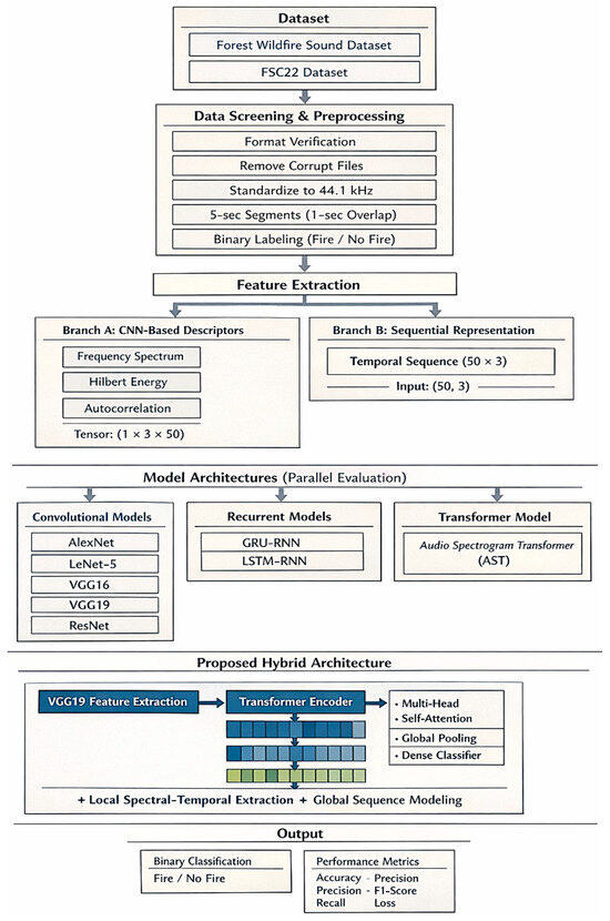
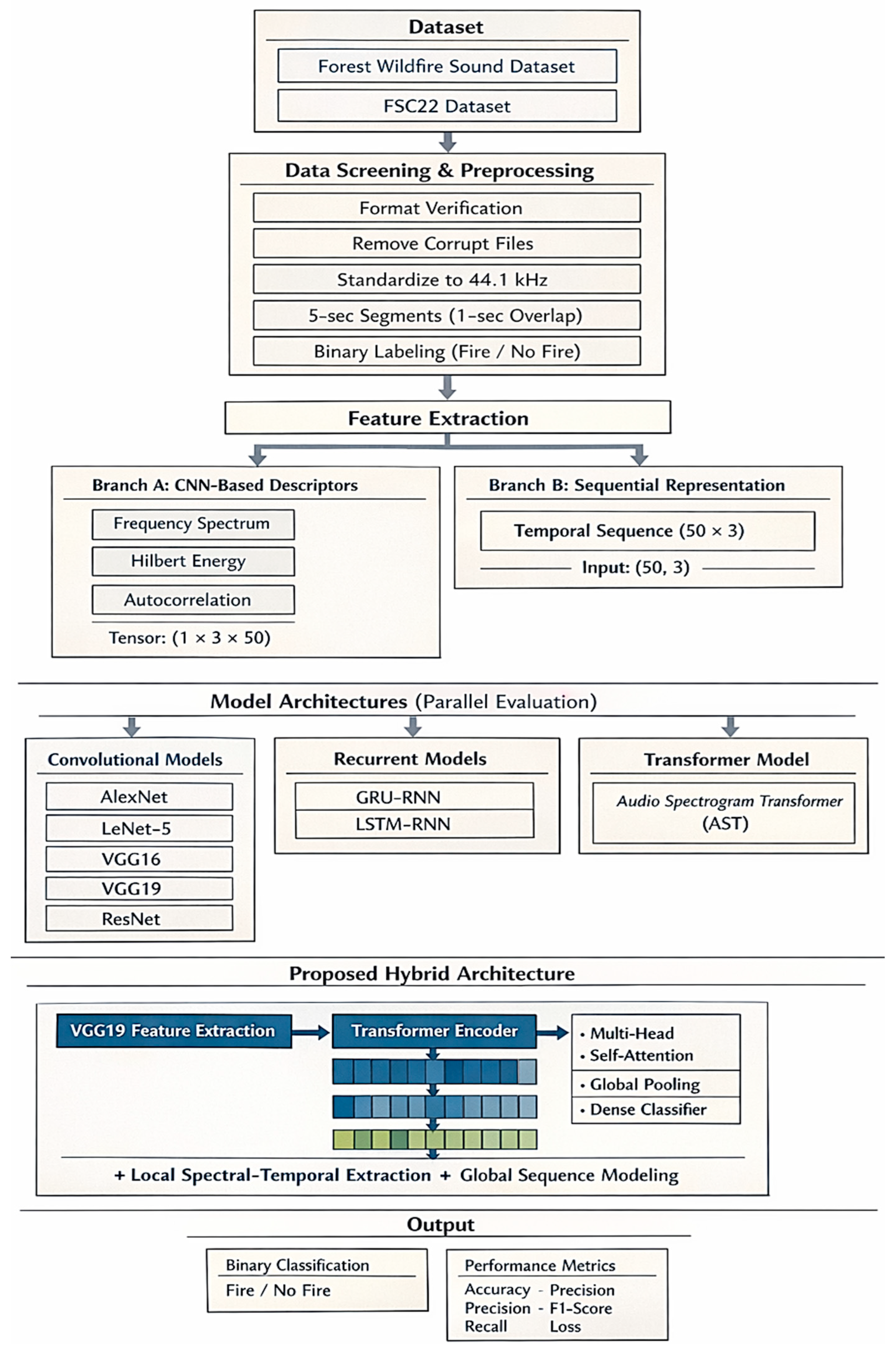
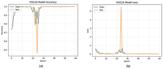
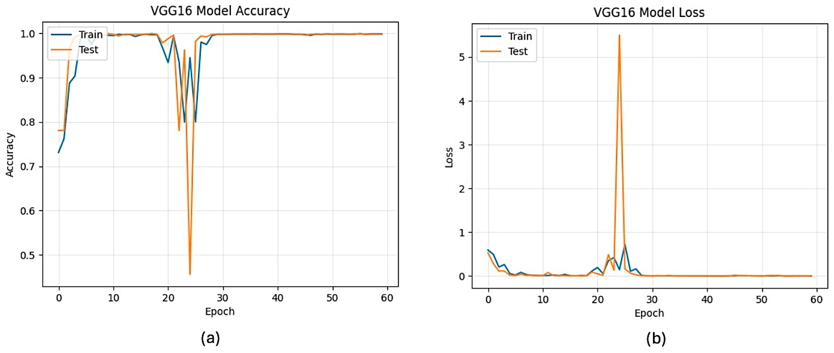
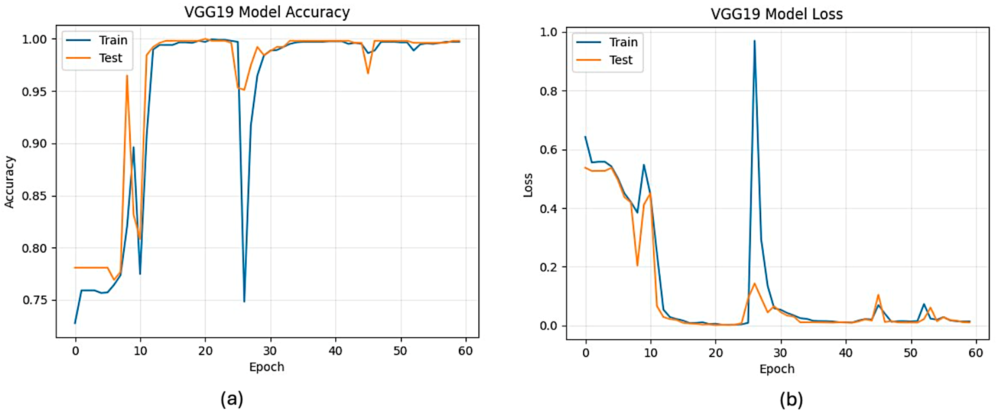
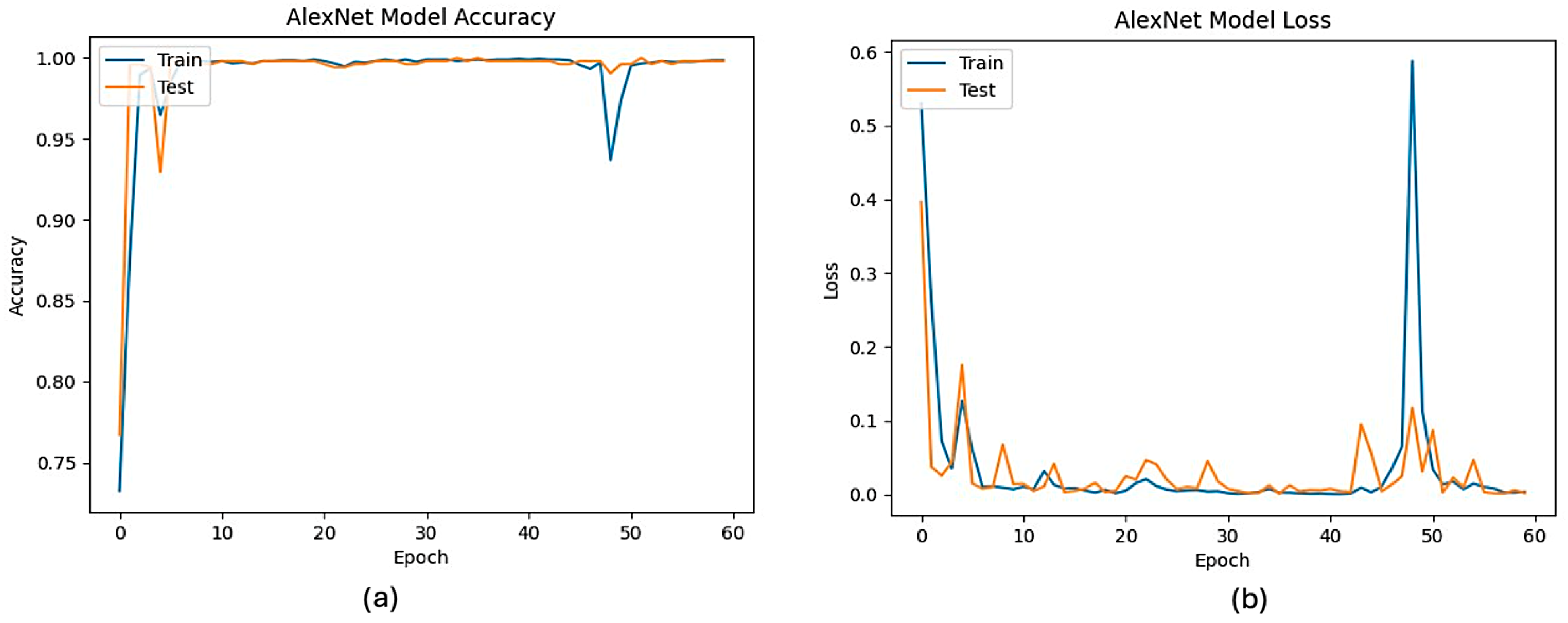
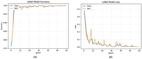
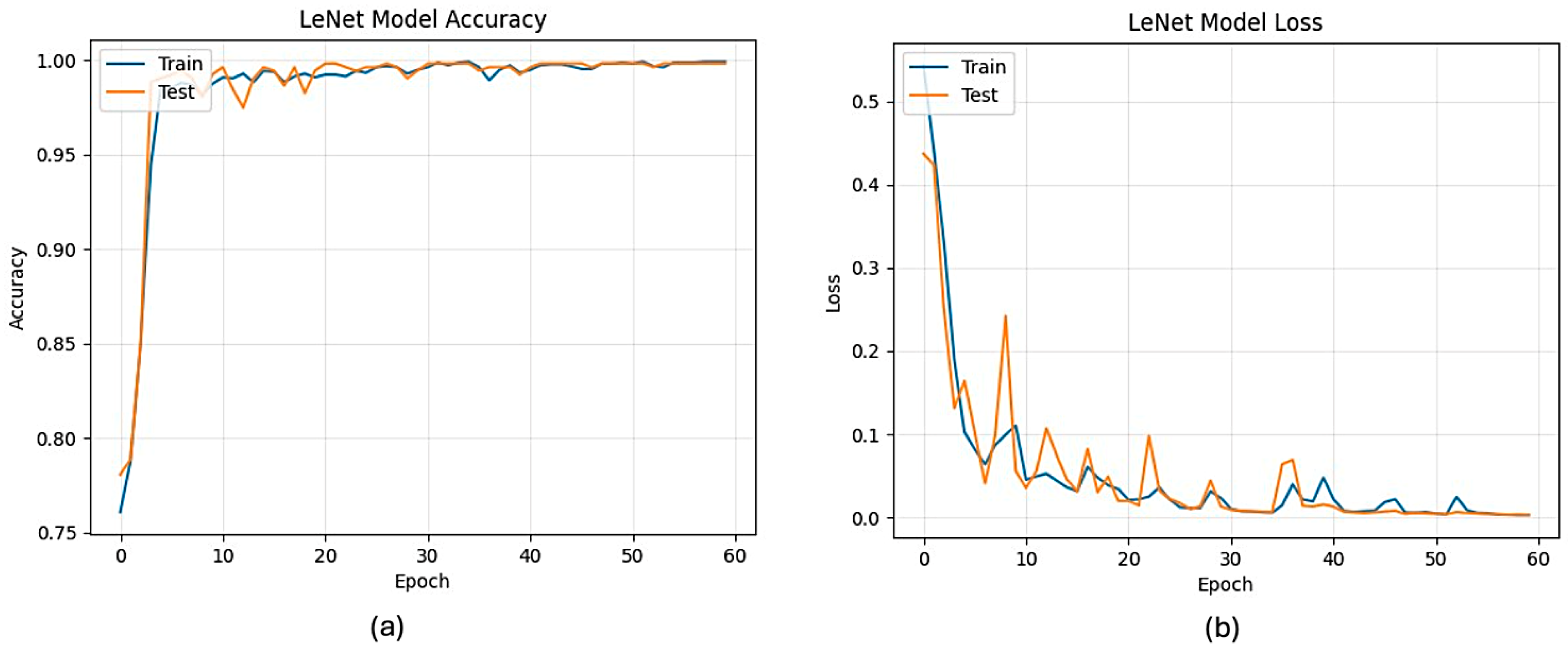
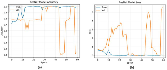
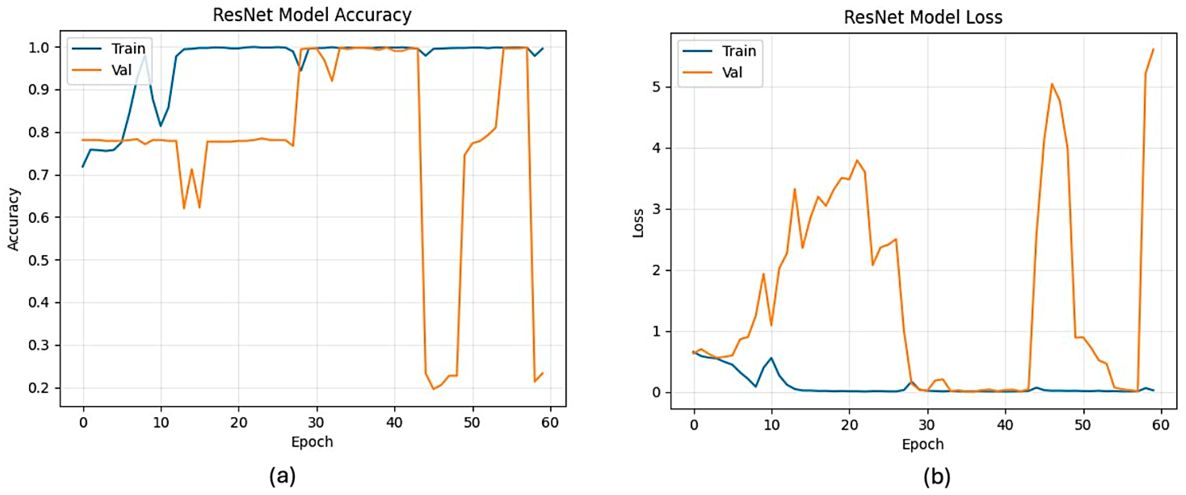
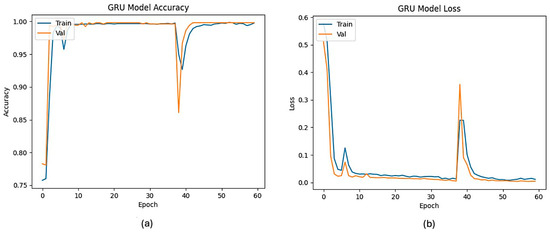
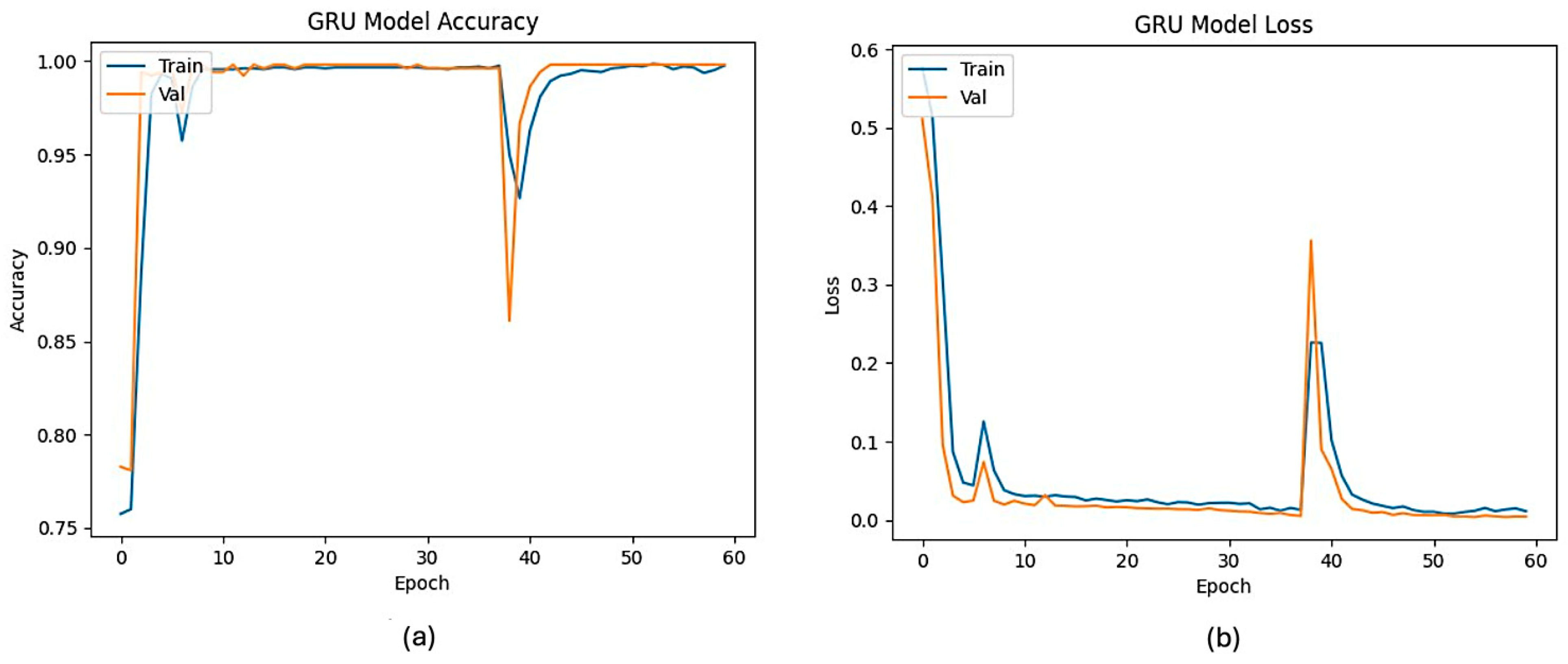
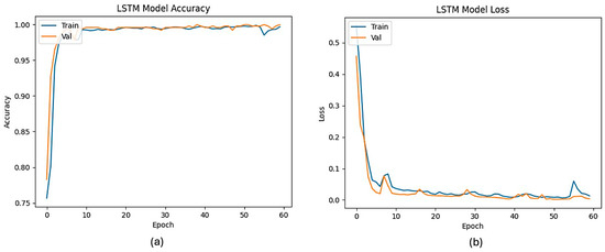
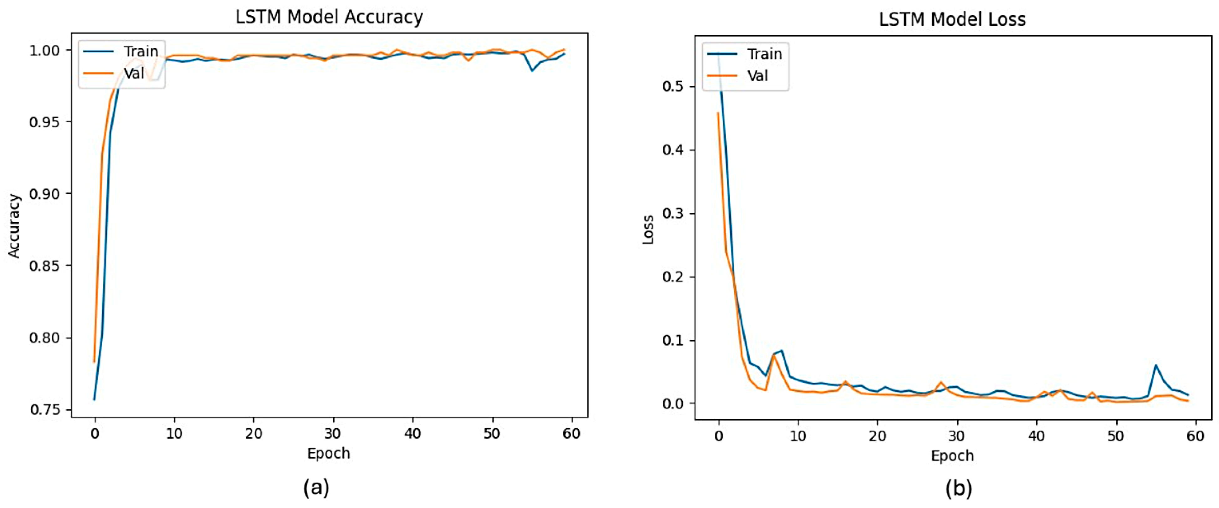
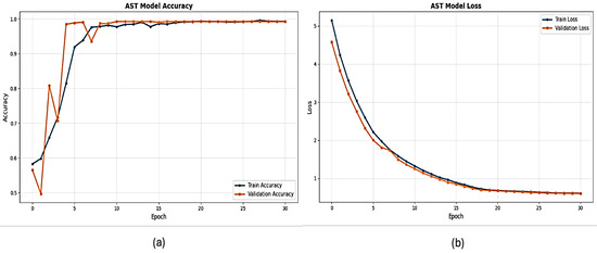
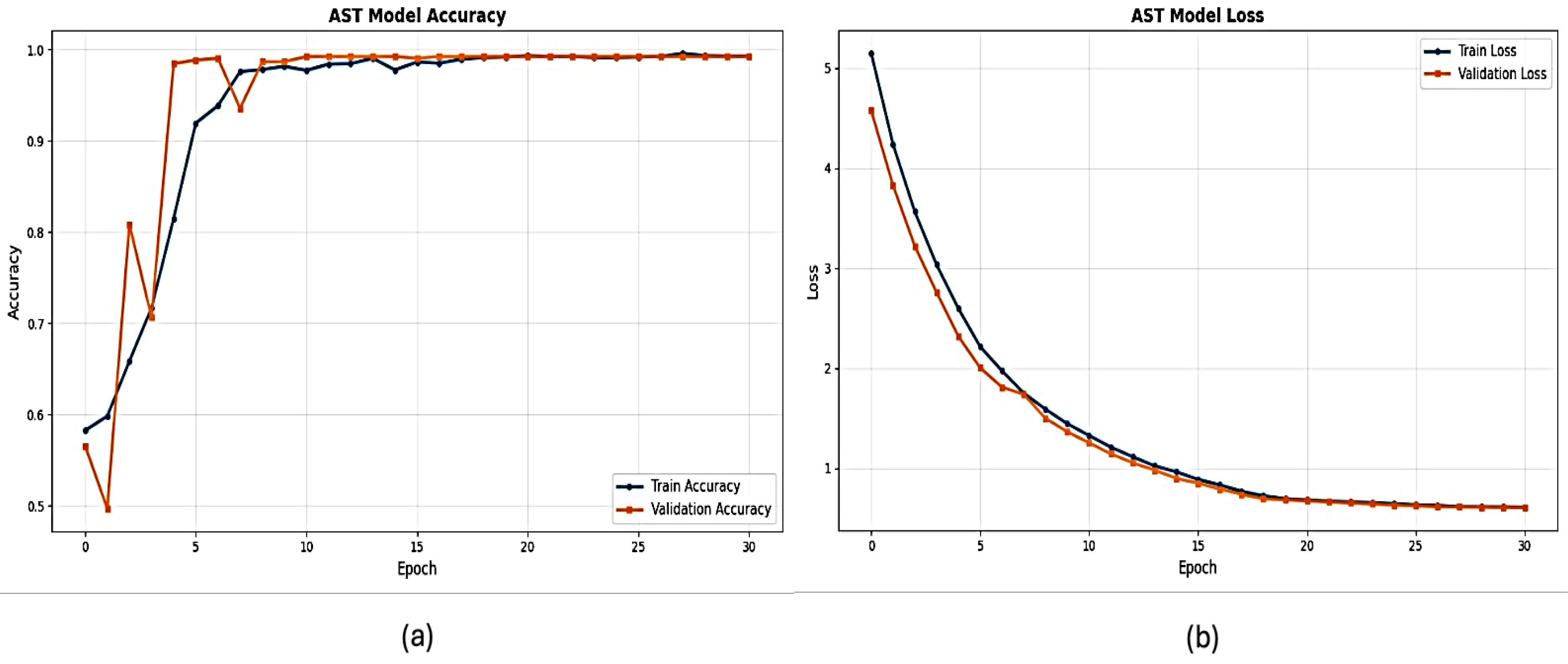
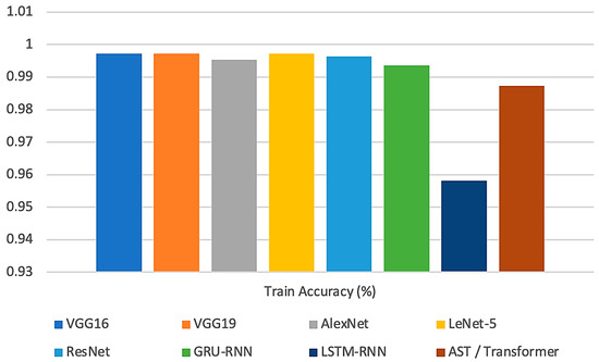
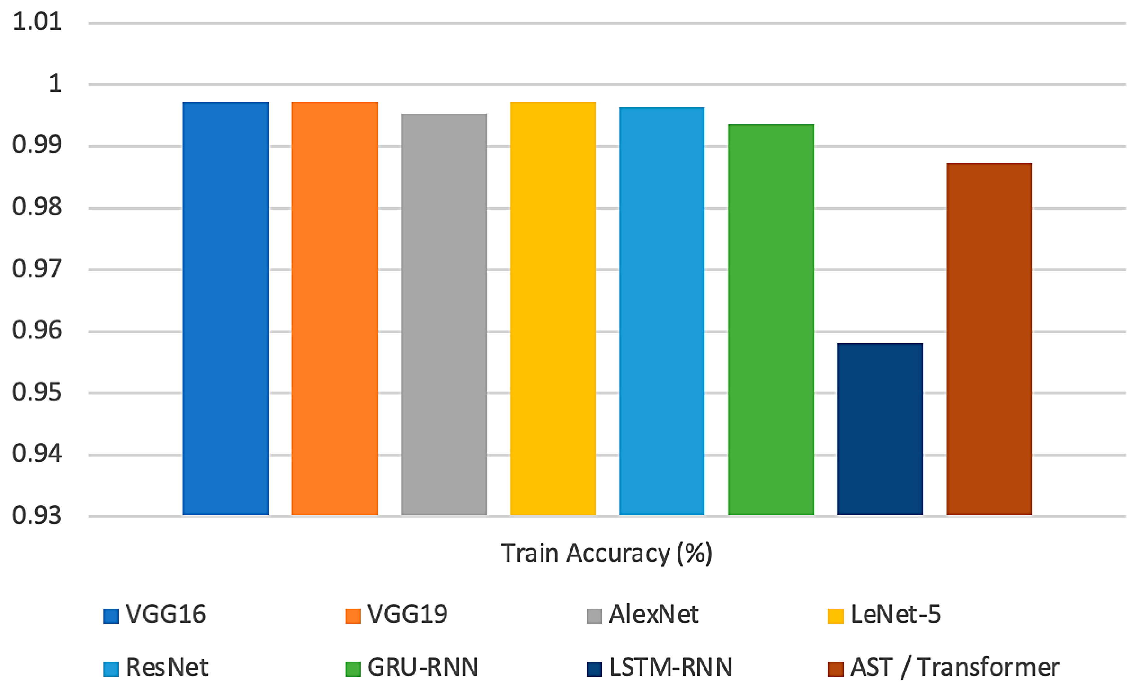
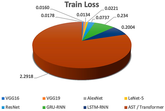
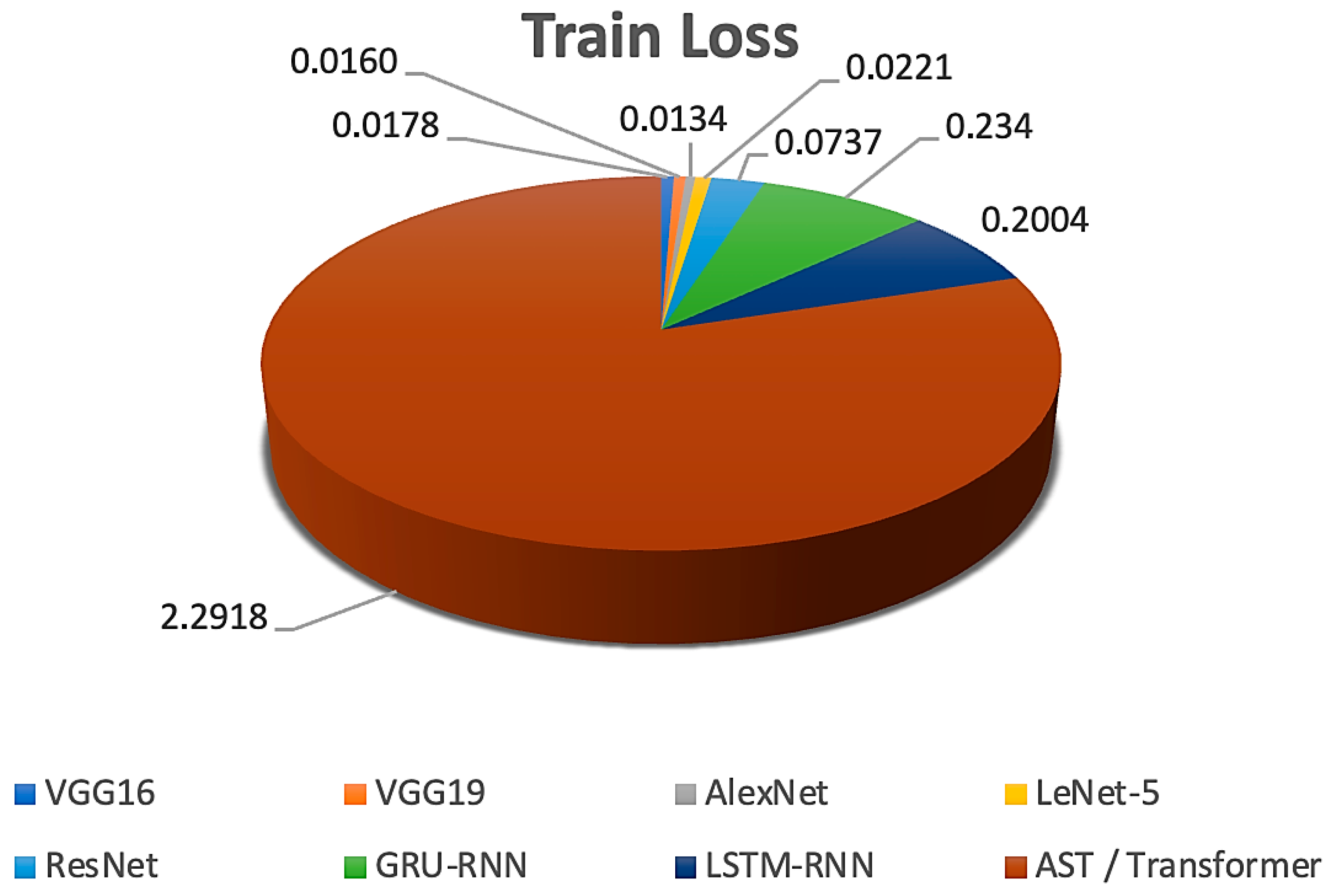
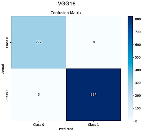
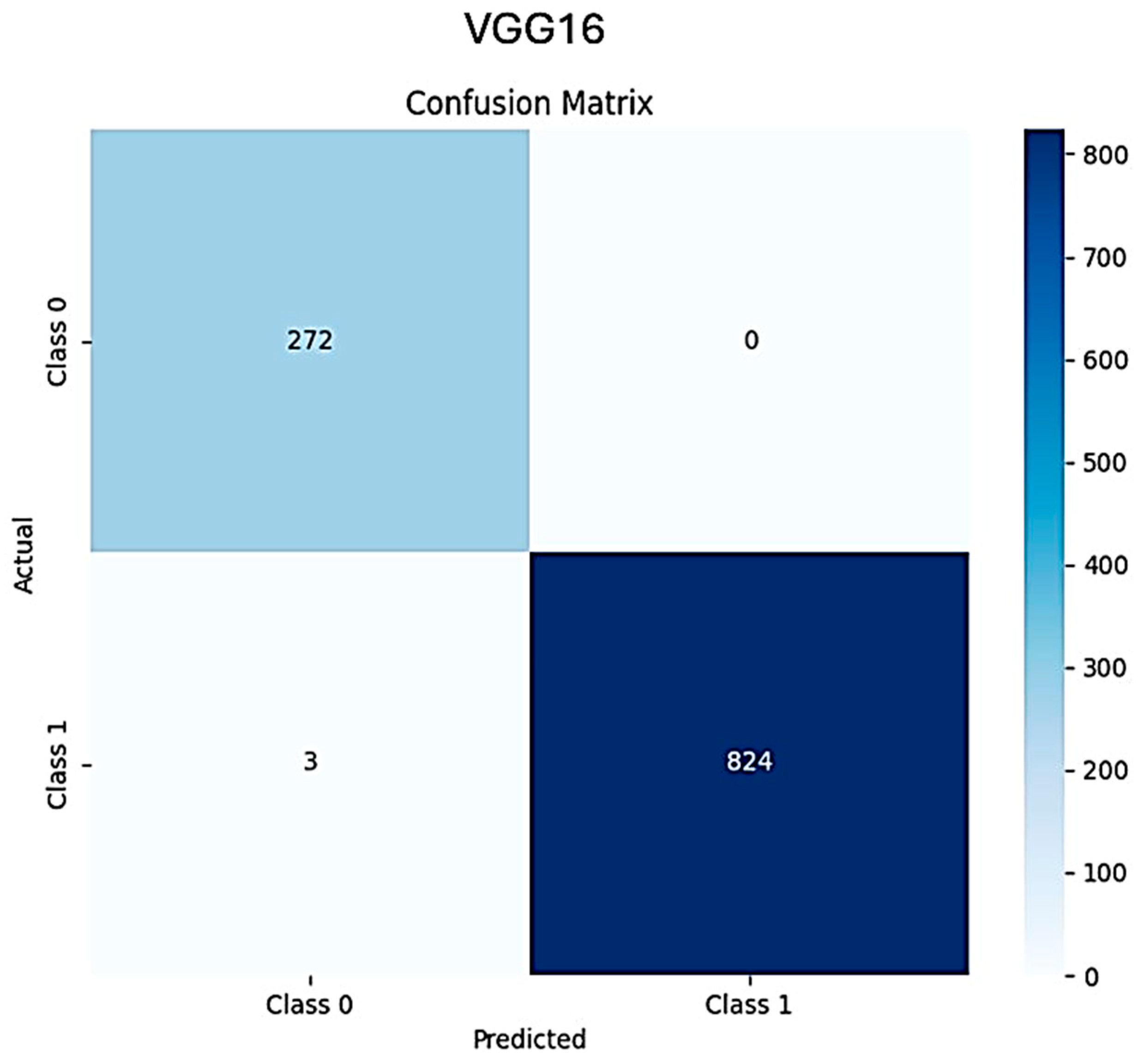
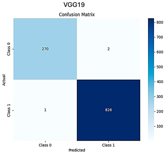
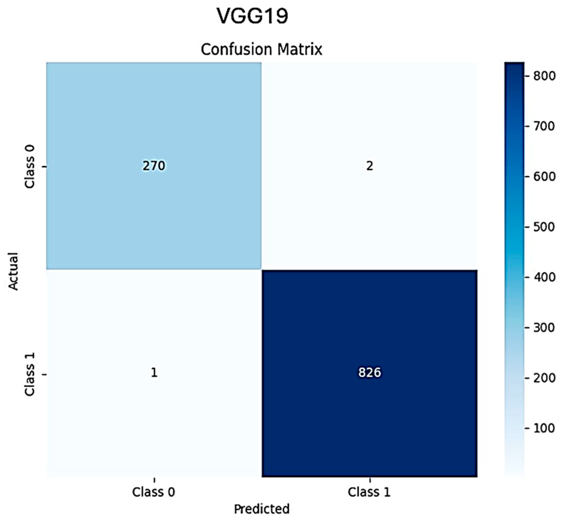
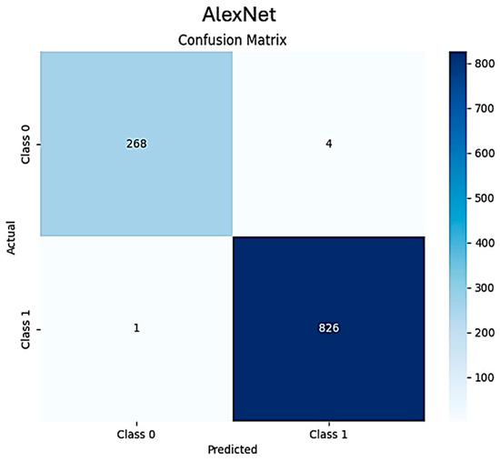
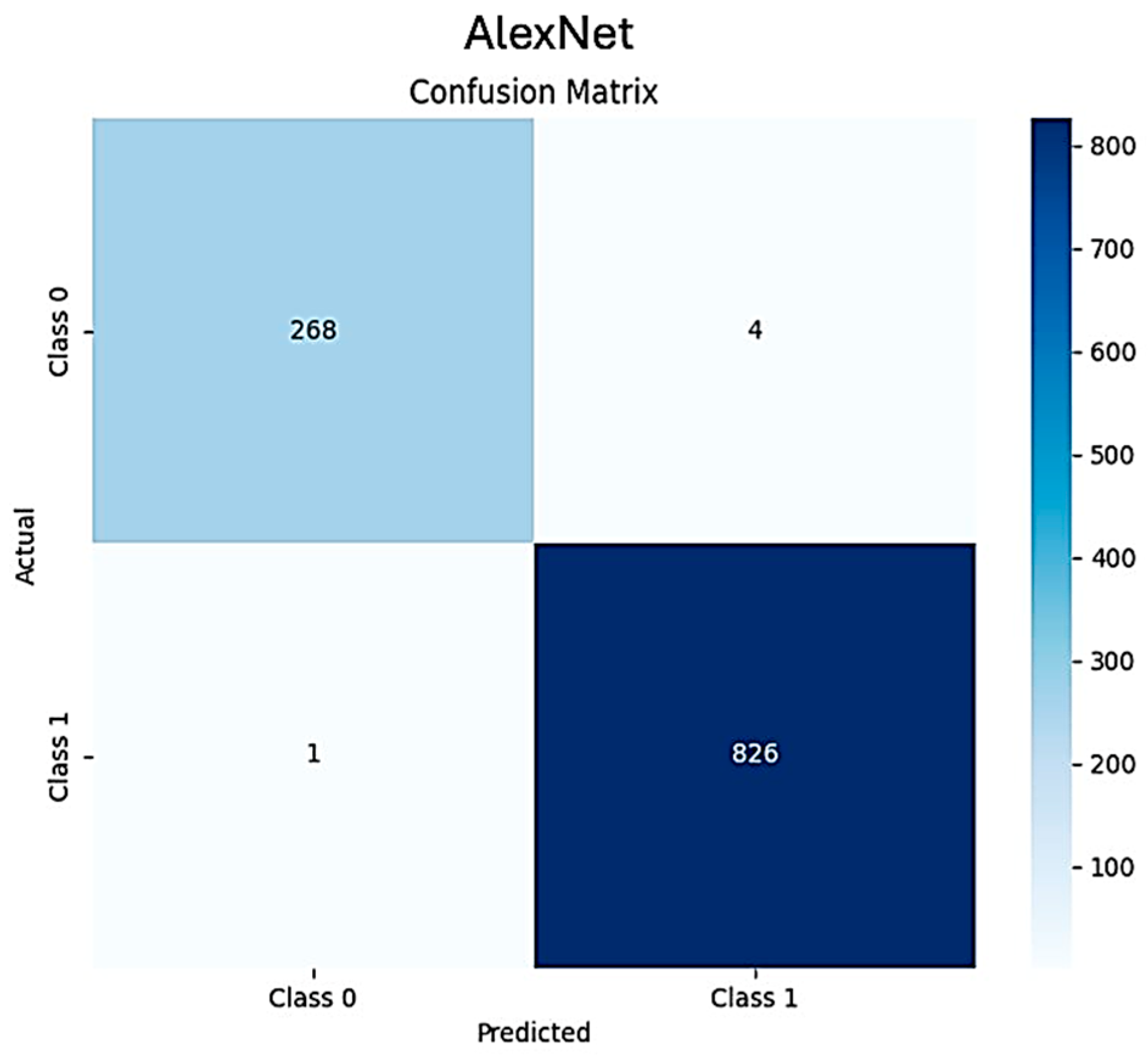
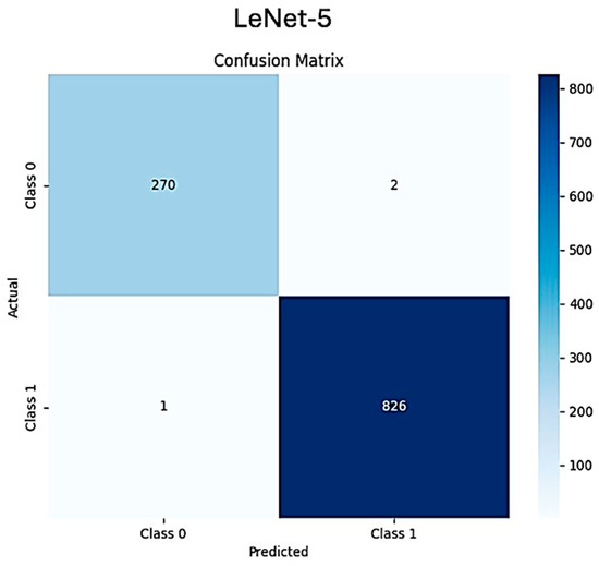
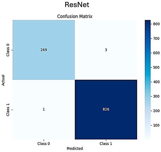
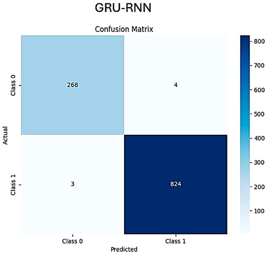
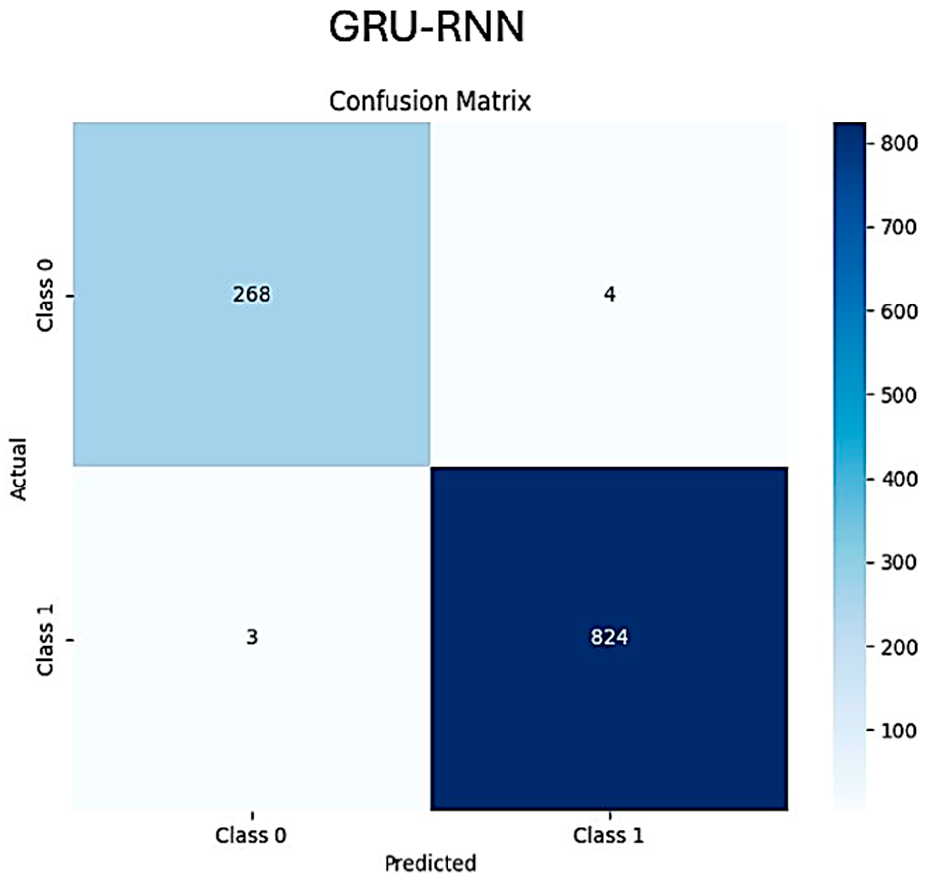
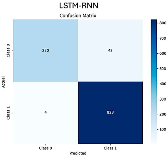
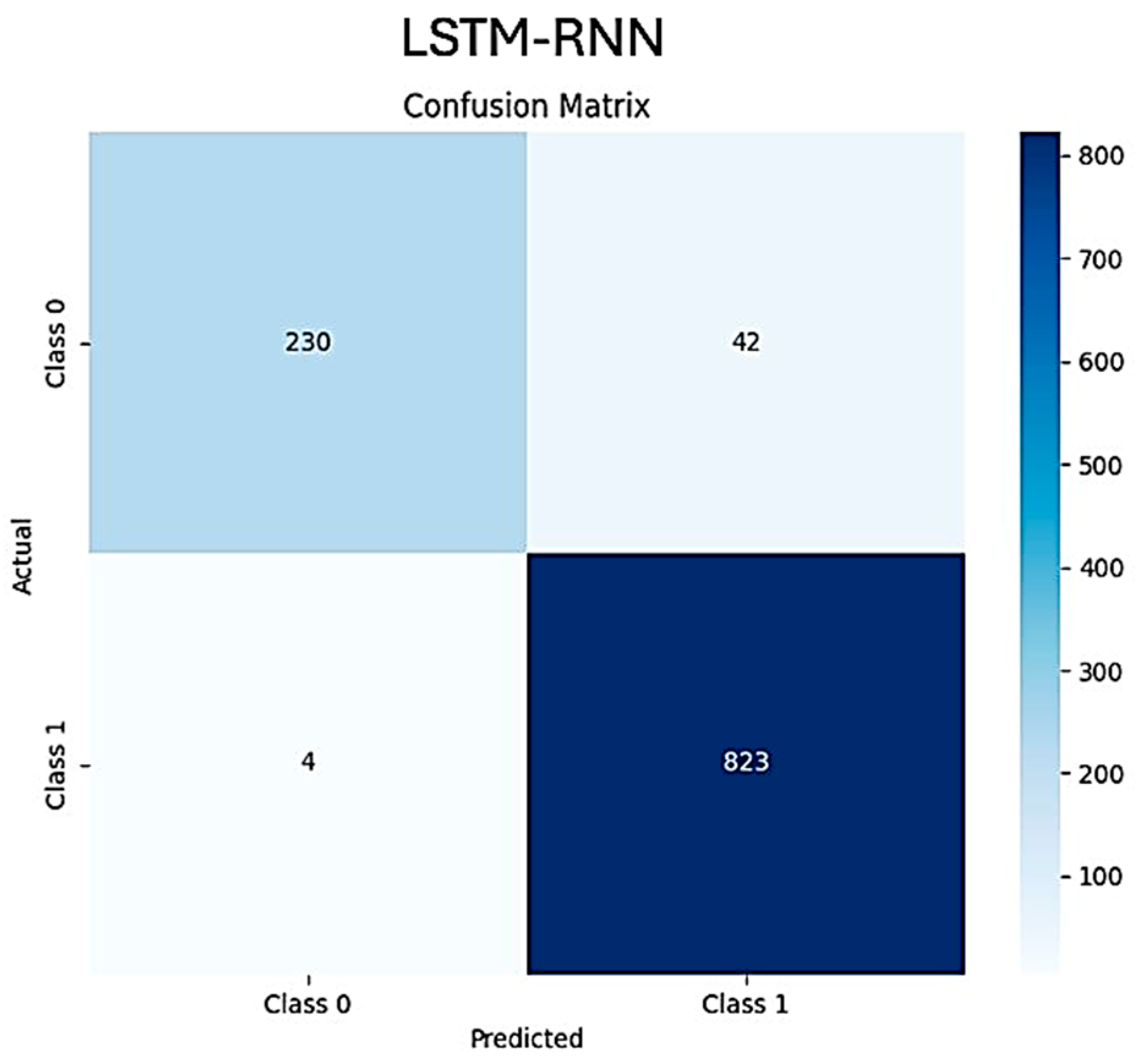
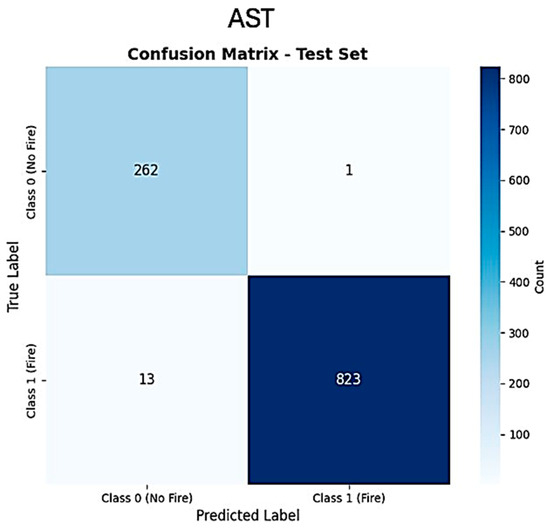
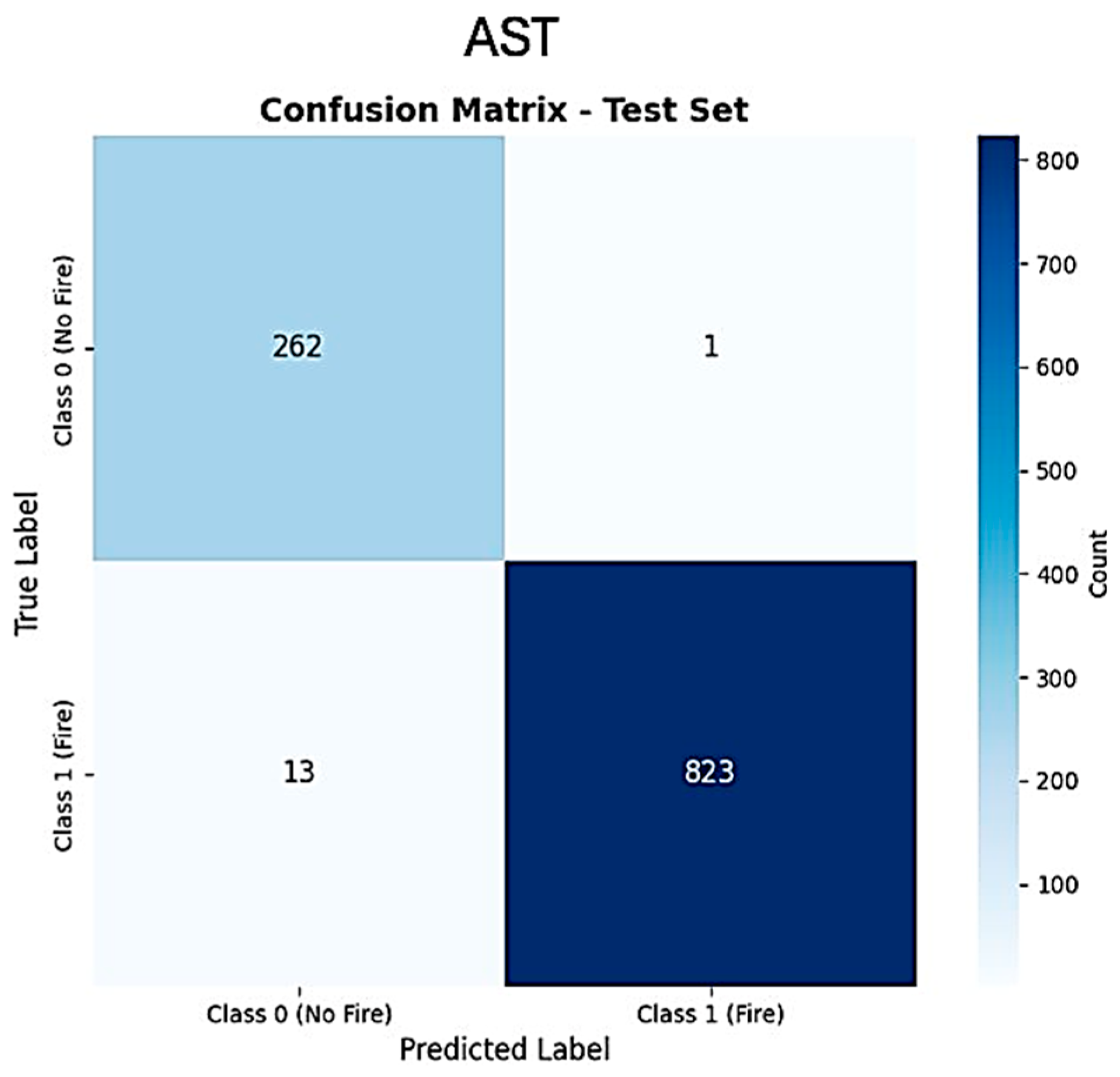
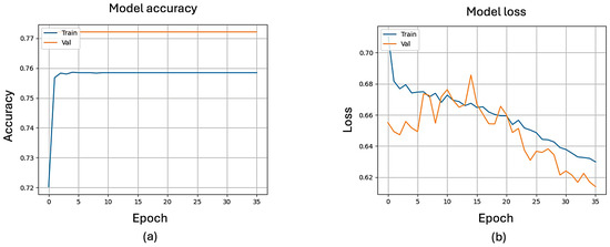
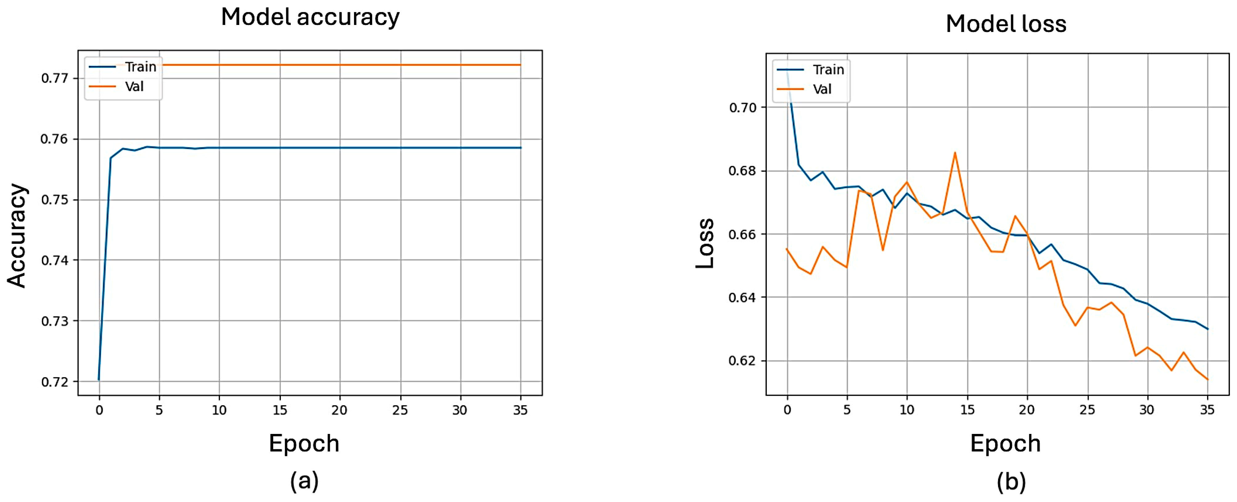
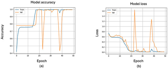
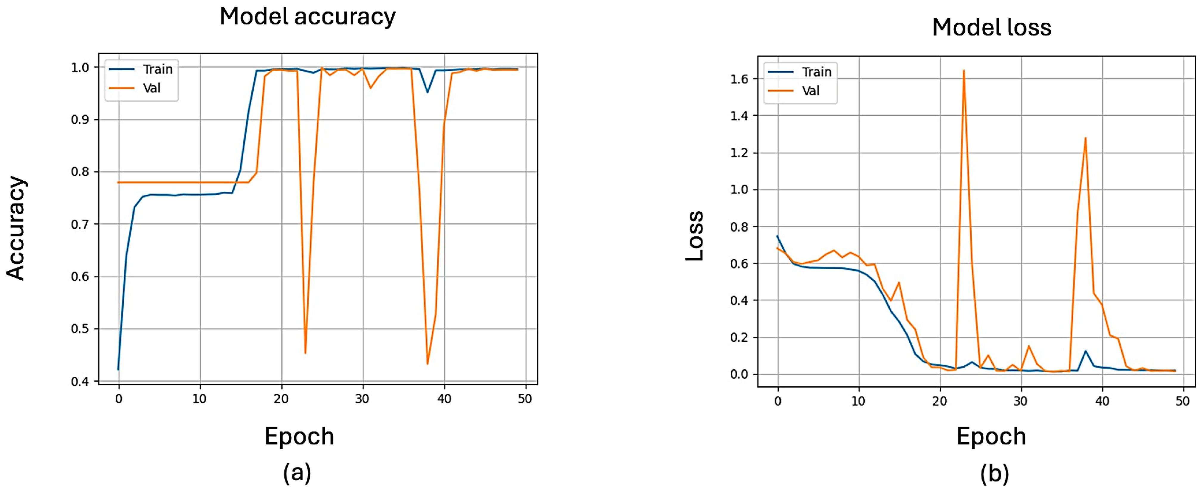
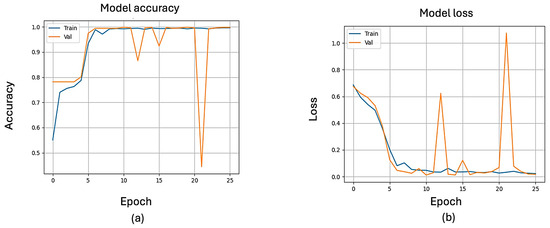
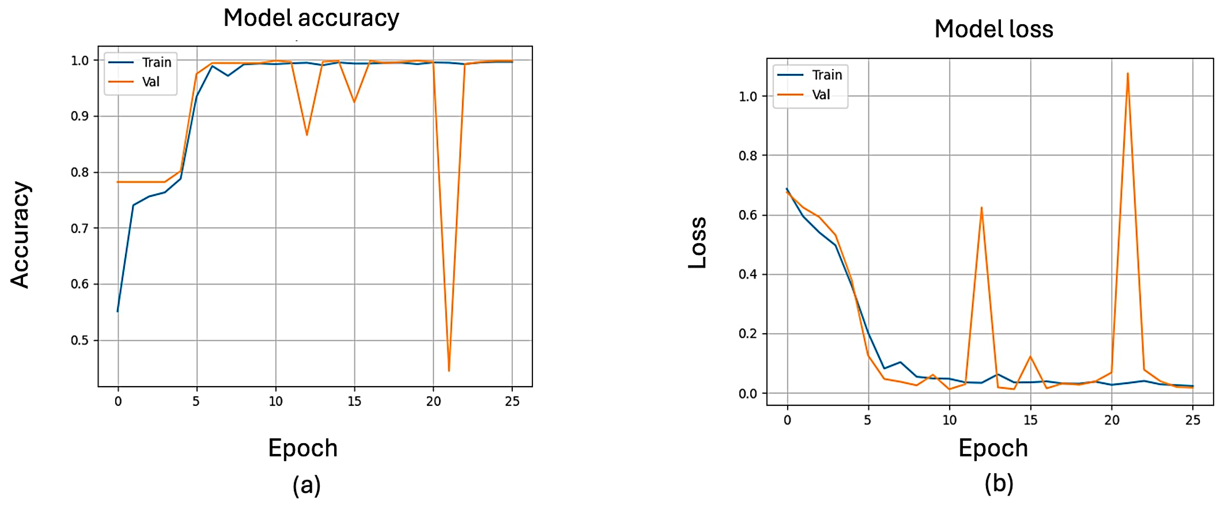
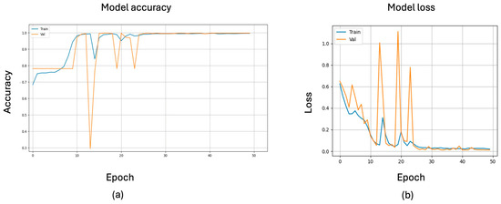
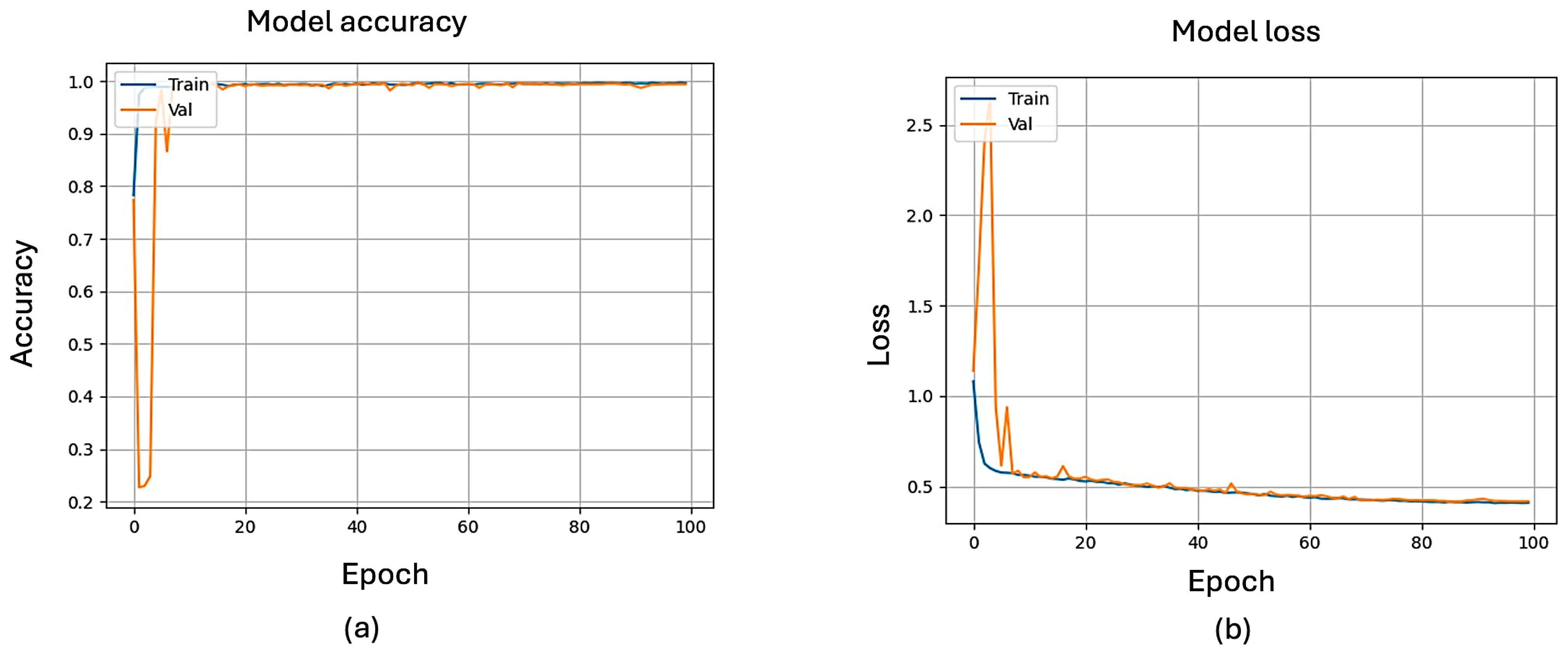

Disclaimer/Publisher’s Note: The statements, opinions and data contained in all publications are solely those of the individual author(s) and contributor(s) and not of MDPI and/or the editor(s). MDPI and/or the editor(s) disclaim responsibility for any injury to people or property resulting from any ideas, methods, instructions or products referred to in the content. |
© 2026 by the authors. Licensee MDPI, Basel, Switzerland. This article is an open access article distributed under the terms and conditions of the Creative Commons Attribution (CC BY) license.