An Improved Sinh Cosh Optimizer Based 2-Degree-of-Freedom Double Integral Feedback PID Controller for Power System Load Frequency Control

Abstract

An improved Sinh Cosh optimizer (ISCHO) is proposed to resolve load frequency control (LFC) tasks. The original Sinh Cosh optimizer (SCHO) employs a fixed iteration-based switching function to balance exploration and exploitation, which lacks awareness of search dynamics and leads to inefficient optimization. Therefore, this paper proposes a “first grabbing then washing” strategy to dynamically balance exploration and development. The proposed ISCHO technique is tested on 13 benchmark functions and compared with Particle Swarm Optimization, Sine Cosine Algorithm, and Grey Wolf Optimizer, demonstrating superior optimization performance. Furthermore, a new controller based on the two-degree-of freedom PID controller (2DOF-PID), the two-degree-of freedom with double integral feedback PID controller (2DOF-PIDF-II), is proposed. A two-area multi-source interconnected power system, incorporating thermal, hydraulic, wind, and solar generation units with nonlinearities (GRC and GDB), uncertainties, and load fluctuations, is employed to validate the proposed approach. Quantitative results under step load perturbation demonstrate that the ISCHO-optimized 2DOF-PIDF-II controller significantly outperforms other methods. For area 1 frequency deviation, ISCHO reduces the maximum overshoot by 38.37%, 19.09%, and 21.48% compared to PSO, SCA, and SCHO. For tie-line power deviation, maximum overshoot is reduced by 53.00% compared to PSO. These results confirm that the proposed ISCHO-tuned 2DOF-PIDF-II controller substantially enhances system frequency stability under various operating conditions.

1. Introduction

In recent years, the power system has become more complex due to load diversification and the widespread use of renewable energy sources (RES). The rapid growth of renewable energy sources (such as solar and wind) leads to increased system inertia, affecting grid stability and increasing frequency deviation [1]. This change makes the imbalance between power supply and demand more prominent, especially in the case of a high proportion of renewable energy access increasing the volatility of power supply, bringing new challenges to the safe operation of the grid.

To deal with these problems, load frequency control (LFC) has become a key means to ensure the stability of the power grid. LFC maintains the frequency of the grid by adjusting the generation and load and controls the power flow of the liaison lines between areas to ensure power balance [2]. It can effectively reduce the frequency deviation and enhance the anti-disturbance ability of the power grid to ensure the safety and stability of the power grid under complex conditions. With the development of the power system, the role of LFC will become more and more important and become the core technology to ensure the operation of the power grid. The preliminary results of this work were previously published in preprint form on Authorea [3].

1.1. Literature Review

With the development of modern control theory, many new controllers have been proposed for power system frequency problems. Robust control [4] is one of them. For example, in reference [5], a hierarchical optimal robust controller is designed using a two-level control strategy; the method is applied to single-area and multi-area interconnected power systems, and better control performance is obtained. In reference [6], a robust LFC strategy based on a disturbance observer is proposed for two-area power systems with stochastic delay perturbations, which can solve the uncertainty problem caused by stochastic delay perturbations. In the LFC problem, the robust control strategy can theoretically cope with the instability problems caused by system disturbance and parameter modeling errors. Still, its order is generally high, the design algorithm is relatively complex, and the degree of dependence on engineering experience is high, so it is difficult to realize in practical applications. Model predictive control (MPC) has been applied in the field of LFC due to its modeling flexibility and better anti-interference ability [7]. Reference [8] proposes a robust deep Koopman MPC method introduced for effective LFC of a nonlinear interconnected power system, which reduces computational burden. In reference [9], the author proposed an adaptive model predictive control method for LFC of two-area interconnected power systems with independent microgrids to solve the frequency deviation caused by system parameter changes and load perturbations. The rolling optimization strategy of MPC has good response performance to the uncertainties caused by perturbations, but it requires a lot of computation, and its robustness and stability for nonlinear and uncertain systems need further study. However, sliding mode control (SMC) can be well applied to nonlinear systems; it not only has a fast response, and small overshoot, but also has good convergence performance [10]. For example, reference [11] applies the hybrid control method based on fuzzy logic and sliding mode theory to the interconnected power system containing wind power generation, and this control method can effectively cope with the high variability and load demand changes in wind power generation. Aiming at the uncertainty and random disturbance in LFC problems, a multi-rate output feedback sliding-mode control scheme based on Event Triggered (ET) was proposed in the literature [12]. The proposed controller was applied to power systems with nonlinear constraints in two areas, and the control scheme was compared with ET. The simulation results show that the proposed control scheme has better response performance.

In a recent study, researchers adopted various controllers to solve the LFC problem. These controllers include, but are not limited to, proportional integral derivative (PID) [13], tilt-integral-differential (TID) [14], fractional-order PID (FOPID) [15], and two-degree-of-freedom PID (2DOF-PID) [16]. These controllers are the most traditional LFC controllers, as described in reference [17]. Reference [18] demonstrates that conventional PID controllers can effectively suppress frequency deviations and tie-line power fluctuations in two-area power systems. However, their one-degree-of-freedom structure limits the ability to simultaneously optimize set-point tracking and disturbance rejection, exhibiting relatively weak robustness to system parameter variations. Reference [19] introduces the TID controller, where the tilt characteristic enhances load disturbance rejection capability and provides superior frequency response compared to traditional PID, though the complexity of fractional-order parameter tuning poses challenges for practical engineering implementation. Reference [20] employs the FOPID controller, where fractional-order integral and derivative orders offer greater design flexibility for more precise adjustment of system dynamic response. Nevertheless, numerical implementation of fractional operators requires approximation, and both theoretical analysis and parameter optimization processes remain relatively complex. Reference [21] adopts the 2DOF-PID controller, whose two-degree-of-freedom structure enables independent optimization of set-point tracking and disturbance rejection, effectively resolving the inherent conflict in traditional one-degree-of-freedom PID. However, the increased number of parameters raises tuning difficulty, and the controller lacks effective high-frequency noise suppression mechanisms.

To overcome the limitations of conventional controller tuning methods, numerous studies have integrated intelligent optimization algorithms with various controller structures to enhance overall LFC system performance through parameter optimization. Reference [22] proposes a cascade PI-(1 + FOPID) controller optimized by the Wild Horse Optimizer (WHO) for interconnected power systems, where the cascade structure enhances disturbance rejection capability and the optimization algorithm improves tuning efficiency. However, this approach increases system complexity and introduces strong coupling between parameters. Reference [23] develops an improved Cheetah optimizer (mCO) to optimize FOPID controller parameters in multi-area systems with renewable energy integration, offering fast convergence speed, though the problem-dependent nature of the improvement strategy limits its generalizability and requires further validation. Reference [24] adopts the Marine Predator Algorithm to optimize a P-P-FOPID controller for two-area interconnected generation systems, demonstrating strong global search capability at the cost of high computational complexity that limits real-time applications. Reference [25] combines the Sine Cosine Algorithm with fuzzy PID control for nonlinear three-area LFC systems, where fuzzy logic effectively handles system nonlinearity and uncertainty, offering good adaptability; however, fuzzy rule base construction relies heavily on expert experience, introducing subjectivity. Reference [26] employs the Imperialist Competitive Algorithm to optimize fuzzy PI controllers for two-area systems, where the combination of fuzzy control and optimization algorithms enhances system robustness, though the numerous algorithm parameters lead to tedious tuning processes. Reference [27] applies the Differential Evolution algorithm to optimize FOPID controllers for three-area systems, offering a simple structure and strong robustness, yet suffering from slow convergence speed and susceptibility to local optima. Reference [28] investigates the application of TID controllers based on the Sine Cosine Algorithm for LFC in two-area hybrid source systems, demonstrating advantages in multi-source energy integration, although hybrid system complexity increases modeling difficulty. Reference [29] proposes a FOPIDN-(1 + PIDN) controller optimized by the Marine Predator Algorithm for interconnected systems with renewable energy sources, where the nested structure enhances control flexibility but the high controller order poses challenges for practical implementation. Reference [30] applies Kharitonov’s theorem to design FOPID controllers for single-area systems, offering theoretical rigor that ensures robust stability under parameter uncertainty; however, the complex design process limits scalability primarily to single-area applications. Reference [31] introduces a TID controller optimized by the Salp Swarm Algorithm (SSA) specifically for LFC systems incorporating Flexible AC Transmission System (FACTS) devices, where consideration of FACTS dynamic characteristics effectively improves transient performance, though FACTS modeling complexity significantly influences algorithm convergence. Reference [32] employs Grey Wolf Optimization to design multi-degree-of-freedom PID controllers for two-area systems, where the enhanced control structure combined with the algorithm’s strong global search capability yields good optimization performance, yet the numerous controller parameters lead to extended optimization time. Reference [33] utilizes the Jellyfish Search Optimizer (JSO) to optimize fractional-order PID gains for two-area hybrid power systems, offering algorithm novelty and high optimization accuracy, though insufficient algorithm stability analysis and limited application cases warrant further investigation. Reference [34] develops a hybrid Improved Artificial Bee Colony and Particle Swarm Optimization (MHABC-PSO) algorithm to address LFC challenges in two-area interconnected systems, where the hybrid approach combines the strengths of both algorithms to achieve good convergence performance, albeit with increased computational burden due to algorithm complexity.

Given the above discussion, hybrid optimization in the context of LFC is still an emerging field, so much research is needed to verify the effectiveness and applicability of various schemes. For the best performance, you must use a powerful optimizer. From the above discussion, the controller with multiple degrees of freedom usually has better performance. At the same time, the author notes that the double feedback integral link significantly improves the system stability, and anti-interference ability effectively eliminates steady-state errors combined with the integral effect and thus achieves optimization in dynamic response, tracking accuracy, and robustness. The structure can not only accelerate the response speed, and suppress overshoot, but also reduce parameter sensitivity and adapt to model uncertainty. This combination of performance enhancement and engineering practicability makes it widely applicable in high-precision demand scenarios such as industrial control and robotics. Therefore, to better control the error caused by the instability of renewable energy, a two-degree-of-freedom PID controller with double integration is proposed in this paper. A Sinh Cosh optimizer (SCHO) has high comprehensibility, strong editable, excellent effect, and great advantages for multi-parameter optimization. Therefore, this paper proposes an improved Sinh Cosh optimizer (ISCHO) based on a Sinh Cosh optimizer. Based on the above, the combination of ISCHO and the 2DOF-PIDF-II controller is proposed in this paper. According to the integral of time multiplied by absolute error (ITAE) criteria (ISCHO: 2DOF-PIDF-II), acting as the controller of the LFC in the test system, we consider various load modes, system uncertainties, and nonlinearities to demonstrate the effectiveness and robustness of the proposed ISCHO: 2DOF-PIDF-II scheme.

1.2. The Novelty and Contributions of This Paper

Compared with the current research on similar topics, the novelty and main contributions of this paper are summarized as follows:

To address frequency deviations caused by intermittency and uncertainty introduced by renewable energy integration, a novel 2DOF-PIDF-II controller structure is proposed for two-area interconnected multi-source power systems incorporating renewable energy sources.

Inspired by the “first grabbing then washing” decision-making wisdom of Go, an improved Sinh Cosh optimizer (ISCHO) is proposed, replacing the original mathematical transition function with a novel exploration–exploitation switching mechanism, thereby enhancing search efficiency and solution quality.

Comprehensive comparative experiments on 13 test benchmark functions systematically verify the superiority and robustness of the ISCHO algorithm compared to the original SCHO and other mainstream algorithms.

The ISCHO algorithm is applied for the first time to optimize the parameters of the 2DOF-PIDF-II controller in LFC problems of two-area interconnected power systems, with performance comparisons against recent algorithms including PSO, SCA, GWO, and SCHO, demonstrating the effectiveness of the proposed method in practical engineering applications.

In designing the proposed 2DOF-PIDF-II controller, multiple practical nonlinear factors are comprehensively considered, including Generation Rate constraints, Governor Dead Band, system uncertainties, communication delays, and load/renewable energy fluctuations, bringing the research closer to engineering reality.

To comprehensively validate the effectiveness and robustness of the proposed controller, multiple testing scenarios are designed including step load perturbation, multistage load perturbation, and random load perturbation, evaluating system frequency regulation performance under complex operating conditions from multiple dimensions.

2. Dynamic Model of Load Frequency Control

2.1. Two-Area Multi-Source Interconnected Power System

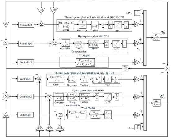
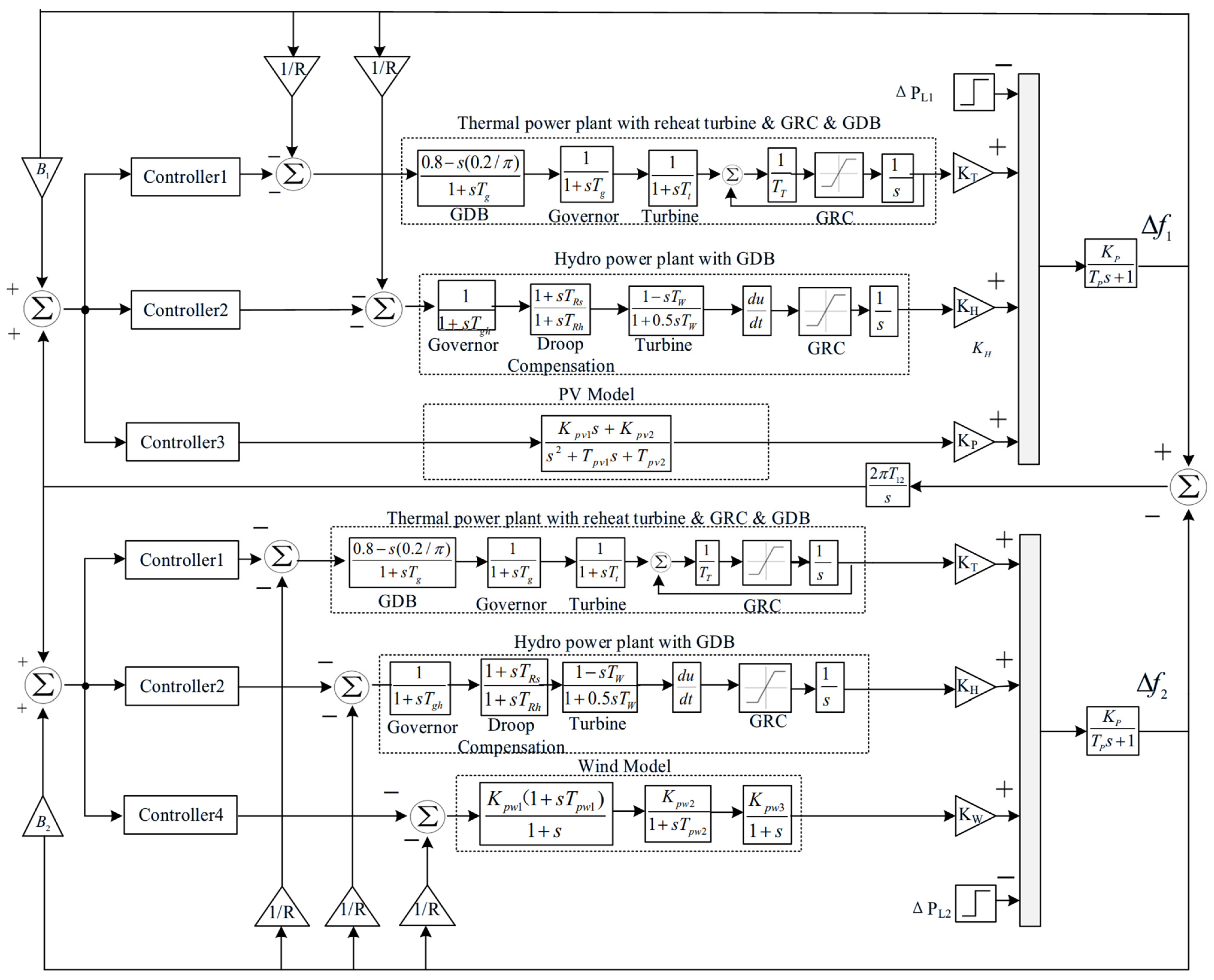
In this paper, we consider a two-area asymmetric power system model with renewable energy sources [35]. Among them, area one is composed of thermal generators, hydroelectric power generation and solar generation, and area two is composed of thermal power generation, hydroelectric power generation and wind generation. Two typical physical constraints, Generation Rate constraint (GRC) and Governor Dead Band (GDB), are considered to load the actual operation of the power system. Both GRC and GDB are shown in Figure 1. GRC represents the closed-loop GRC of the thermal power generation unit and the open-loop GRC of the hydro power generation unit, respectively. The closed-loop GRC is controlled by TT, and the transfer function of GDB can be expressed as GDB = (N1 + sN2)/1 + sTg. The change rate of GRC is 10% P.U./min (0.0017 P.U.MW/s). The GRC of the hydropower station is 270% P.U./min (0.045 P.U.MW /s) [36]. Each zone has a power rating of 2000 MW and a nominal load of 1740 MW, of which thermal power units provide 1000 MW, hydropower units provide 500 MW, and solar and wind power units provide 240 MW. The block diagram of the two-area asymmetric power system model with new energy is shown in Figure 1. The specific parameters in the model are shown in Table 1.

Figure 1. Two-area power system structure model.

Table 1. Parameters specific to the analyzed power system.

Parameter	Value	Parameter	Value
KP	68.9655 Hz/P.U.MW	Tpv1	100 s
TP	11.49 s	Tpv2	50 s
R	2.4 Hz/P.U.MW	Kpwl	1.25
Tg	0.06 s	Tpwl	6 s
Tt	0.3 s	Kpw2	1.4
Tgh	0.2 s	Tpw2	0.41 s
TRs	4.9 s	Kpw3	1
TW	1.1 s	T12	0.0433 P.U.MW/rad
TRh	28.749 s	TT	0.3 s
Kpv1	−18	N1	0. 8
Kpv2	900	N2	0.2/π

2.2. The Proposed Power System Controller

As the penetration rate of renewable energy continues to increase, the power system is facing multiple challenges such as decreased inertia, complex disturbance characteristics, and variable operating conditions. Traditional load frequency control methods struggle to strike a balance between rapid frequency recovery and strong disturbance suppression. Especially when dealing with continuous low-frequency disturbances and random fluctuations, they often exhibit large steady-state deviations, slow regulation speed, and significant overshoot, seriously affecting the frequency stability and power supply quality of the system. Moreover, due to the inherent limitations of its single-degree-of-freedom structure, the parameter tuning of traditional PID controllers often requires a compromise between tracking performance and anti-disturbance capability, making it difficult to simultaneously meet the dual requirements of modern power systems for dynamic response and robustness.

To address the issues, this paper proposes a novel two-degree-of-freedom PID controller with double integral feedback (2DOF-PIDF-II). This controller systematically enhances the comprehensive performance of load frequency control through structural innovations, with its key distinctions from conventional 2DOF-PID and PIDF-II controllers articulated as follows:

First, in contrast to the single-degree-of-freedom structure of the conventional PIDF-II, the proposed controller adopts a two-degree-of-freedom decoupling architecture, which independently optimizes set-point tracking performance and disturbance rejection capability through separate feedback and feedforward channels. This design fundamentally overcomes the inherent contradiction in traditional PID tuning where fast tracking and strong disturbance rejection cannot be simultaneously achieved. Second, regarding the integral action design, unlike the single-integral structure of conventional 2DOF-PID controllers, the proposed controller introduces a double-integral feedback mechanism. While retaining the traditional integral’s capability to eliminate steady-state errors, this mechanism further enhances the system’s ability to suppress persistent low-frequency disturbances, such as slow load drifts and renewable energy fluctuations. Third, to address the issue of high-frequency noise interference, an adjustable filter is integrated into the derivative channel, effectively attenuating noise measurement and improving control signal smoothness and engineering practicality—a capability that conventional 2DOF-PID controllers lack.

Therefore, the proposed 2DOF-PIDF-II controller can achieve rapid frequency control under complex operating conditions, effectively suppress various load disturbances, and significantly enhance the robustness of the system when parameters change. In summary, by combining the flexible decoupling capability of the 2DOF architecture, the enhanced anti-interference ability of the dual integration effect, and the noise attenuation effect of the filter elements, the proposed controller provides an effective solution for frequency stability control in power systems under high renewable energy integration.

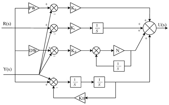
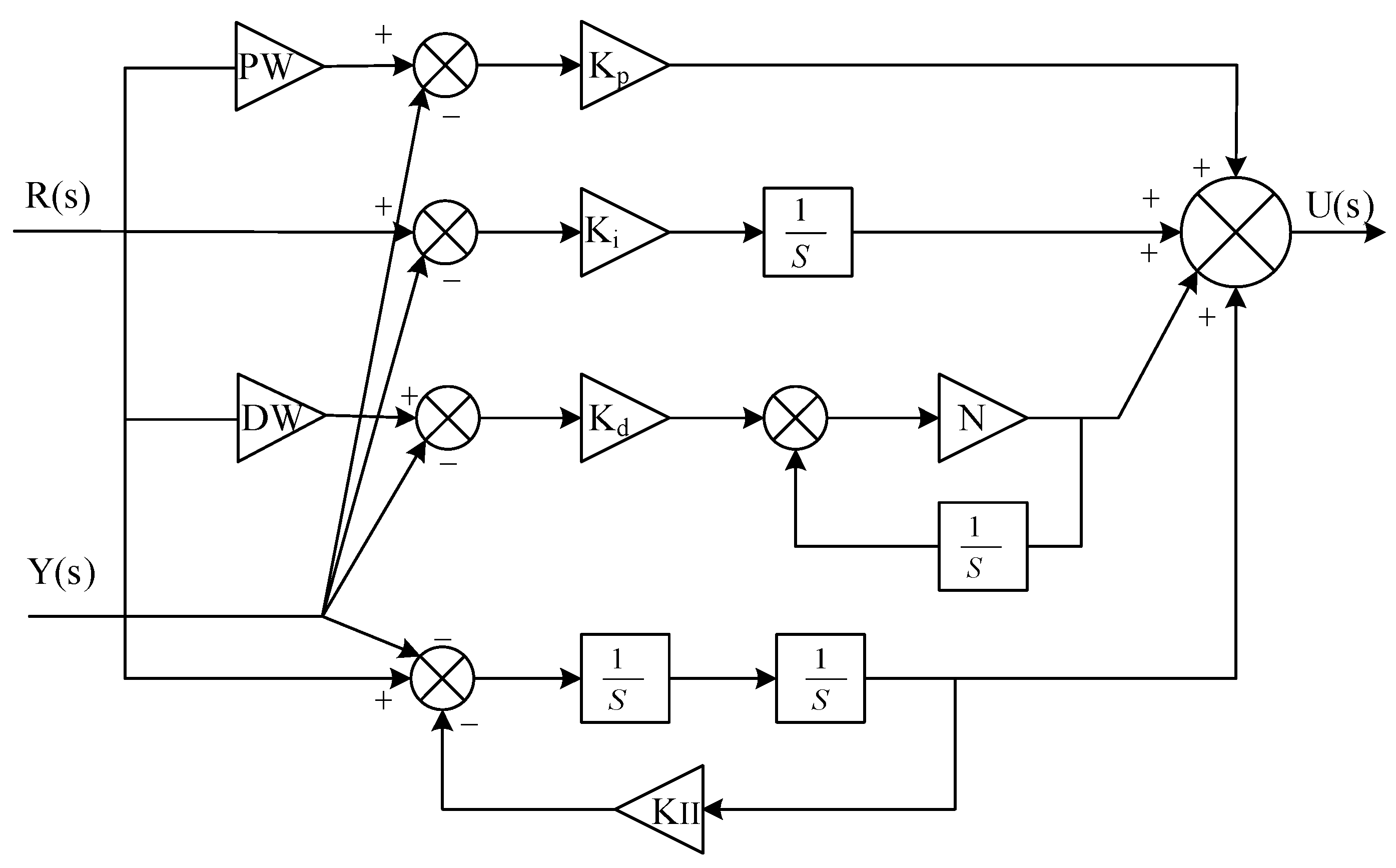
The basic structure of the controller is shown in Figure 2, where two separate loops can be seen. Two inputs are applied to the controller: one is the reference, and the other is the output of the system. The error signal caused by the difference between the two signals is used by the controller to generate the controller output signal, which consists of the proportional part, the integral part, the derivative part and the double integral part according to its weight. The mathematical formula of the 2-degree-of-freedom PID controller with the filter and double integral is as follows:

$$u=K_p((PW)r-y)+{\displaystyle \frac{K_I}{s}}(r-y)+{\displaystyle \frac{K_{D}sN}{s+N}}((DW)r-y)+{\displaystyle \frac{K_{II}}{s^2}}(r-y)$$

(1)

where r and y are the two input signals, and r is the reference and y is the output of the system. K_p, K_i, K_d, N and K_II are proportional gain, integral gain, differential gain, filter coefficient and double integral feedback gain, respectively. u is the output of the controller. PW and DW are the proportional section weights and derivative section weights of the controller.

Figure 2. 2DOF-PIDF-FII controller model.

The effect of the filter coefficient is like a low-pass filter, which can reduce the high-frequency sensor noise and system oscillation in the power system. In this paper, the double integral feedback gain K_II is connected with an integral link to form a negative feedback system. When the areal control error signal passes through the negative feedback, the areal control error signal is weakened, thus improving the sensitivity of the controller, reducing the overshoot of the system and making the system stable.

By converting the mathematical formula derived from Equation (1) to the Laplace domain, we can get Equation (2).

$$U(s)=K_p\left(PW\cdot R(s)-Y(s)\right)+{\displaystyle \frac{K_I}{s}}\left(R(s)-Y(s)\right)+{\displaystyle \frac{K_{D}Ns}{s+N}}\left(DW\cdot R(s)-Y(s)\right)+{\displaystyle \frac{K_{II}}{s^2}}\left(R(s)-Y(s)\right)$$

(2)

By rearranging the above equation, the terms containing R(s) are grouped into the feedforward part, and the terms containing Y(s) are grouped into the feedback part. This results in Equation (3).

$$U(s)=\left[K_{p}PW+{\displaystyle \frac{K_I}{s}}+{\displaystyle \frac{K_{D}Ns}{s+N}}DW+{\displaystyle \frac{K_{I}I}{s^2}}\right]R(s)-\left[K_p+{\displaystyle \frac{K_I}{s}}+{\displaystyle \frac{K_{D}Ns}{s+N}}+{\displaystyle \frac{K_{II}}{s^2}}\right]Y(s)$$

(3)

Therefore, the feedforward transfer function C_r(s) and the feedback transfer function C_y(s) are as follows:

$$C_r(s)=K_{p}PW+{\displaystyle \frac{K_I}{s}}+{\displaystyle \frac{K_{D}Ns}{s+N}}DW+{\displaystyle \frac{K_{II}}{s^2}}$$

(4)

$$C_y(s)=-\left(K_p+{\displaystyle \frac{K_I}{s}}+{\displaystyle \frac{K_{D}Ns}{s+N}}+{\displaystyle \frac{K_{II}}{s^2}}\right)$$

(5)

Let the transfer function of the controlled object be G_p(s). The structure of the closed-loop system is $Y(s)=G_p(s)U(s)+D(s)$. Here, D(s) represents external disturbances, specifically load variations. In actual physical systems, load disturbance ΔP_L is applied at the input or output end of the generator-load link. Usually, its effect can be equivalent to a disturbance applied at the output end of G(s), or it can be included in the transfer function of the generator load. To analyze closed-loop stability, we assume ΔP_L to be 0 because stability is independent of external inputs and is only related to the closed-loop poles. And U(s) is

$$U(s)=C_r(s)R(s)+C_y(s)Y(s)$$

(6)

Substituting this gives Equation (7).

$$Y(s)=G_p(s)\left[C_r(s)R(s)+C_y(s)Y(s)\right]\left[\begin{array}{c}1-G_p(s)C_y(s)\end{array}\right]Y(s)=G_p(s)C_r(s)R(s)$$

(7)

Therefore, the closed-loop output of the system is as follows:

$$Y(s)={\displaystyle \frac{G_p(s)C_r(s)}{1-G_p(s)C_y(s)}}R(s)$$

(8)

Since C_y(s) itself contains a negative sign, −C_y(s) > 0 (for positive gain). To make it more intuitive, let us define the following:

$$H(s)=-C_y(s)=K_p+{\displaystyle \frac{K_I}{s}}+{\displaystyle \frac{K_{D}Ns}{s+N}}+{\displaystyle \frac{K_{II}}{s^2}}$$

(9)

From this, we can obtain Equation (10).

$$1-G_p(s)C_y(s)=1+G_p(s)H(s)$$

(10)

Then the closed-loop output of the system can be derived as follows:

$$Y(s)={\displaystyle \frac{G_p(s)C_r(s)}{1+G_p(s)H(s)}}R(s)$$

(11)

where H(s) is the feedback controller and C_r(s) is the feedforward controller.

The characteristic equation is

$$1+G_{plant}(s)H(s)=0$$

(12)

Taking the LFC system model of a one-area with non-reheat steam turbine as an example and ignoring external disturbances at the same time, the following can be obtained:

$$G_p(s)={\displaystyle \frac{K_P}{(1+s{T}_g)(1+s{T}_t)(1+s{T}_P)}}$$

(13)

Substituting into the characteristic equation yields Equation (14):

$$1+{\displaystyle \frac{K_P}{(1+s{T}_g)(1+s{T}_t)(1+s{T}_P)}}\left(K_p+{\displaystyle \frac{K_I}{s}}+{\displaystyle \frac{K_{D}Ns}{s+N}}+{\displaystyle \frac{K_{II}}{s^2}}\right)=0$$

(14)

By factoring out the common denominator from the above expression, we can obtain the following:

$$s^2(s+N)(1+s{T}_g)(1+s{T}_t)(1+s{T}_P)+K_P\left[K_p{s}^2(s+N)+K_{I}s(s+N)+K_{D}N{s}^3+K_{I}I(s+N)\right]=0$$

(15)

Expand and organize into a descending power polynomial of s:

$$b_6{s}^6+b_5{s}^5+b_4{s}^4+b_3{s}^3+b_2{s}^2+b_{1}s+b_0=0$$

(16)

The respective coefficients are as follows:

$$\begin{array}{c}{b}_6=T_g{T}_t{T}_P\\ b_5=(T_g{T}_t+T_g{T}_P+T_t{T}_P)+N{T}_g{T}_t{T}_P\\ b_4=(T_g+T_t+T_P)+N(T_g{T}_t+T_g{T}_P+T_t{T}_P)\\ b_3=1+N(T_g+T_t+T_P)+K_P(K_p+K_{D}N)\\ b_2=N+K_P(K_{p}N+K_I)\\ b_1=K_P(K_{I}N+K_{II})\\ b_0=K_P{K}_{II}N\end{array}$$

(17)

Equation (16) is a sixth-order characteristic polynomial, and the positions of its roots determine the stability of the closed-loop system.

For a sixth-order system, the Routh array is constructed as follows:

s6	b6	b4	b2	b0
s5	b5	b3	b1	0
s4	c1	c2	c3
s3	d1	d2	0
s2	e1	e2
s1	f1	0
s0	g1

The calculation of the auxiliary coefficient is as follows:

$$\begin{array}{c}{c}_1={\displaystyle \frac{b_5{b}_4-b_6{b}_3}{b_5}},\hspace{1em}{c}_2={\displaystyle \frac{b_5{b}_2-b_6{b}_1}{b_5}},\hspace{1em}{c}_3=b_0\\ d_1={\displaystyle \frac{c_1{b}_3-b_5{c}_2}{c_1}},\hspace{1em}{d}_2={\displaystyle \frac{c_1{b}_1-b_5{c}_3}{c_1}}\\ e_1={\displaystyle \frac{d_1{c}_2-c_1{d}_2}{d_1}},\hspace{1em}{e}_2=c_3\\ f_1={\displaystyle \frac{e_1{d}_2-d_1{e}_2}{e_1}},\hspace{1em}{g}_1=e_2\end{array}$$

(18)

According to the stability criterion of the closed-loop system, the sufficient and necessary condition for the asymptotic stability of system Equation (16) is that all elements in the first column of the Routh table are positive, that is,

$$b_6>0,\hspace{1em}{b}_5>0,\hspace{1em}{c}_1>0,\hspace{1em}{d}_1>0,\hspace{1em}{e}_1>0,\hspace{1em}{f}_1>0,\hspace{1em}{g}_1>0$$

(19)

Substituting this formula into Equation (18) will yield an invisible constraint.

$$\begin{gathered} b_5{b}_4>b_6{b}_3 \\ {c}_1{b}_3>b_5{c}_2 \end{gathered}$$

(20)

Meanwhile, through numerical analysis, it was found that for typical power system parameters, the double-integration gain needs to satisfy the following:

$$K_{II}<{\displaystyle \frac{1+N(T_g+T_t+T_P)}{K_P{N}^2{T}_g{T}_t{T}_P}}\cdot \eta$$

(21)

Here, A represents the safety factor, which is usually set between 0.1 and 0.3.

Substituting the power system parameters into the calculation and considering all constraints, the condition for system stability is as follows:

$$0<K_{II}<1.847$$

(22)

2.3. Improved Sinh and Cosh Optimizer

In the original Sinh Cosh optimizer (SCHO), the trade-off between exploration and exploitation is governed by a predefined switching function. This function generates a value that evolves with the iteration count: when the value exceeds 1, the algorithm prioritizes exploration across the solution space; when it drops below 1, the algorithm transitions toward exploitation in a promising space. Although mathematically straightforward, this mechanism relies on a fixed functional form to dictate the search behavior throughout the optimization process. Consequently, it lacks the capacity to perceive critical search dynamics such as population diversity, convergence status, or the topological characteristics of the fitness landscape. The transition between exploration and exploitation proceeds according to a predetermined schedule, irrespective of whether the population has prematurely converged or remains sufficiently diverse. This rigidity often results in suboptimal performance on complex optimization problems: an unnecessarily prolonged exploration phase may delay convergence in early stages, while a premature shift to exploitation can entrap the algorithm in local optima during later stages.

To overcome this fundamental limitation, this paper proposes an improved Sinh Cosh optimizer (ISCHO), which introduces a novel “first grabbing then washing” strategy to replace the fixed-function switching mechanism of the original SCHO. This strategy is conceptually inspired by a classic strategy in the game of Go, often described as “grabbing first then washing” wherein players initially secure territorial advantages through broad positioning before refining their advantages with precise local moves. Analogously, ISCHO adopts this sequential decision-making approach: in the early stage, the “grabbing” operation performs extensive sampling across the search space to identify promising regions and candidate solutions; in the later stage, the “washing” operation conducts fine-grained local optimization around the retained high-quality solutions. Unlike the original SCHO, which mechanically follows a predefined exploration–exploitation schedule based solely on iteration count, ISCHO dynamically adapts its search behavior in response to the evolving quality and distribution of solutions. This adaptive mechanism, drawing inspiration from the strategic wisdom inherent in Go, establishes a more balanced and interpretable trade-off between global exploration and local exploitation, thereby enhancing convergence accuracy and overall robustness in complex optimization tasks.

By constructing a state evaluation system of corner superiority, Edge Diffusion degree, and central latent strength, an intelligent decision function is designed, enabling the algorithm to adaptively switch search modes based on the real-time distribution status of the population—in the early stage, it focuses on local depth development to “grab land” for rapid convergence, and in the middle and later stages, it shifts to guided global exploration to “wash the pattern” to escape local optima. This improvement endows the SCHO algorithm with the ability of state perception and adaptive strategy, achieving dynamic and precise balance between exploration and exploitation and significantly enhancing the algorithm’s convergence speed, solution accuracy, and robustness.

The SCHO optimization algorithm is a recently proposed meta-heuristic algorithm. SCHO includes four aspects: exploration, development, switching mechanism and bounded search strategy. Like other metaheuristic algorithms, SCHO begins by initializing a group of candidate solutions randomly, as illustrated in Equation (23):

$$X=\left[\begin{array}{ccccc}{x}_{\mathrm{1,1}}& \dots & x_{1,j}& x_{1,dim-1}& x_{1,dim}\\ x_{21}& \dots & x_{2,j}& \dots & x_{2,dim}\\ \dots & \dots & x_{i,j}& \dots & \dots \\ ⋮& ⋮& ⋮& ⋮& ⋮\\ x_{N-\mathrm{1,1}}& \dots & x_{N-1,j}& \dots & x_{N-1, \mathit{dim} }\\ x_{N,1}& \dots & x_{N,j}& x_{N, \mathit{dim} -1}& x_{N, \mathit{dim} }\end{array}\right]$$

(23)

where X_i,j is the jth position of ith solution, N is the number of candidate solutions, dim is the dimension of the problem, and X is a set of random candidate solutions obtained via X = rand (N, dim) × (ub − lb) + lb. In the latter definition, rand is a random value within [0, 1], whereas ub and lb are upper and lower bounds, respectively.

When t < T, it is the exploration and development of the first stage, where Max iteration is the maximum iteration value, floor is the rounded function in MATLAB 2023a, and ct is the coefficient of setting the two-phase switch point, which is fixed as 3.6 according to the experiment in this paper. T is expressed as $T=$ floor $\left({\displaystyle \frac{ \mathit{Max}\text{\_}\mathit{iteration} }{ct}}\right)$. In the first stage, the outside of the search space near the location of the search agent is explored in early iterations, and then the search agent gradually approaches the optimal solution. The position update function of the first stage exploration is proposed as follows:

$$X_{(i,j)}^{t+1}=\left\{\begin{array}{c}{X}_{best}^{(j)}+r_1\times W_1\times X_{(i,j)}^t,r_2>0.5\\ X_{best}^{(j)}-r_1\times W_1\times X_{(i,j)}^t,r_2<0.5\end{array}\right.$$

(24)

where t represents the current iteration, and $X_{(i,j)}^{t+1}$ and $X_{(i,j)}^t$ represent the jth position of the ith solution in the current iteration and the next iteration, respectively. $X_{best}^{(j)}$ is the position of the jth best solution obtained so far, and r₁ and r₂ are the random numbers within [0, 1]. W₁ is the weight coefficient of $X_{(i,j)}^t$ in the first exploration stage. In order to control the candidate solution in the first stage away from itself, the exploration is gradually moved toward the optimal solution. It is described as $W_1=r_3\times a_1\times \left(cosh{r}_4+0.388\times sinh{r}_4-1\right)$. Here, r₃ and r₄ are random numbers within [0, 1] and $a_1=3\times \left(-1.3\times {\displaystyle \frac{t}{ \mathit{Max}\text{\_}\mathit{iteration} }}+\mathit{m}\right)$. The development formula for the first stage is as follows:

$$X_{(i,j)}^{t+1}=\left\{\begin{array}{l}{X}_{best}^{(j)}+r_5\times W_2\times X_{(i,j)}^t,r_6>0.5\\ X_{best}^{(j)}-r_5\times W_2\times X_{(i,j)}^t,r_6<0.5\end{array}\right.$$

(25)

r₅ and r₆ are random numbers in the range of [0, 1]. W₂ is the first stage development stage $X_{(i,j)}^t$ weight coefficient, expressed as $W_2=r_7\times a_1\times \left(cosh r_8+0.388\times sinh r_8\right)$, where r₇ and r₈ are random numbers in the range [0, 1].

When t > T, it is the exploration and development of the second stage. The exploration formula of the second stage is as follows:

$$X_{(i,j)}^{t+1}=\left\{\begin{array}{l}{X}_{(i,j)}^t+\left|0.003\times W_3\times X_{best}^{(j)}-X_{(i,j)}^t\right|, r_9>0.5\\ X_{(i,j)}^t-\left|0.003\times W_3\times X_{best}^{(j)}-X_{(i,j)}^t\right|, r_9<0.5\end{array}\right.$$

(26)

W₃ is the weight coefficient of $X_{(i,j)}^t$ in the second stage of exploration, expressed as $W_3=r_{10}\times 2\times \left(-{\displaystyle \frac{t}{ \mathit{Max}\text{\_}\mathit{iteration} }}+0.5\right)$, where r₉ and r₁₀ are random numbers in the range of [0, 1]. The development formula for the second stage is as follows:

$$X_{(i,j)}^{t+1}=X_{(i,j)}^t+r_{11}\times {\displaystyle \frac{sinh r_{12}}{cosh r_{12}}}\left|W_3\times X_{best}^{(j)}-X_{(i,j)}^t\right|$$

(27)

r₁₁ and r₁₂ are random numbers in the range of [0, 1].

In order to better balance exploration and development, this paper proposes a strategy of “first grabbing then washing”. The grabbing is exploration and the washing is development.

Go, as an ancient strategic game, demonstrates a “first grabbing then washing” tactic that embodies profound wisdom in phased resource allocation and risk control: in the early stage, priority is given to obtaining stable gains (“grab territory”); in the middle and later stages, the advantages accumulated in the early stage are utilized to engage in global competition (“wash the overall situation”). Based on this strategic thought, this paper proposes a novel adaptive decision-making mechanism. The concept of “corners, edges, and center” in Go is mapped to the evaluation indicators for the search state in optimization problems. A simple yet effective dynamic decision function is designed to achieve intelligent switching between the “grab” and “wash” search modes.

To mathematize the above ideas, we defined three core state indicators to describe the distribution and quality characteristics of the population in the search space.

Corner Dominance (CD): This metric measures the stability of an algorithm in obtaining high-quality solutions in the boundary regions of the search space (similar to the “corners” in Go). The faster the convergence and the higher the quality of the optimal solution, the larger the CD value, indicating a richer “territory” that can be exploited further. The formula is as follows:

$$C(t)={\displaystyle \frac{\bar{f}(t)-f_{\mathrm{best} }(t)}{\bar{f}(t)+ϵ}}$$

(28)

Among them, $f_{\mathrm{best} }(t)$ represents the current optimal fitness value, $\bar{f}(t)$ represents the average fitness value of the population, and $\mathsf{ϵ}$ is a small constant used to prevent division by zero.

Edge Diffusion (ED): Measures the extent of the distribution of a population in the transitional area within the search space (similar to the “edges” in Go). The more dispersed the population individuals are, the larger the ED value will be, indicating a broader “external force” and creating conditions for “washing”. Its formula is as follows:

$$E(t)={\displaystyle \frac{1}{N(N-1)}}{\sum }_{i\ne j}{\displaystyle \frac{‖x_i-x_j‖}{D_{max}}}$$

(29)

Among them, $D_{max}$ represents the diagonal length of the search space and is used for normalization.

Central Potential (CP): Measures the potential for the central area of the search space (similar to the “center” in Go) to remain underexplored. The closer the center of the current population is to the physical center and the quality of solutions in this area is unknown, the higher the CP value will be, indicating a greater “central pattern” potential and thus worth “washing in”. Its formula is as follows:

$$M(t)={\displaystyle \frac{{min}_{\mathit{boundary} } \Vert c(t)-b\Vert }{R}}$$

(30)

Among them, c(t) represents the geometric center of the population, b represents the boundary point, and R represents the characteristic radius of the search space.

Based on this, we have created the grabbing tendency function G(t) and the washing tendency function W(t).

$$\begin{array}{c}G(t)={\alpha }_1\cdot C(t)+{\alpha }_2\cdot (1-E(t))+{\alpha }_3\cdot (1-\tau )\\ W(t)={\beta }_1\cdot (1-C(t))+{\beta }_2\cdot E(t)+{\beta }_3\cdot M(t)+{\beta }_4\cdot \tau \end{array}$$

(31)

Among them, $\tau =t/T_{\mathit{max}}$ represents the normalized iteration progress; ${\alpha }_i,{\beta }_i$ is the weight coefficient, which is set as (0.4,0.3,0.3) and (0.3,0.3,0.2,0.2), respectively, according to the experiment.

Based on the final decision function D(t), the algorithm switches to different search modes. The formula is as follows:

$$\begin{gathered} D(t)=\left\{\begin{array}{c}GRAB,ifG(t)-W(t)>b(t)\\ WASH,otherwise\end{array}\right. \\ b(t)=\left\{\begin{array}{c}+0.1,\tau <0.3\\ \mathrm{0,0.3}\le \tau <0.7\\ -0.1,\tau \ge 0.7\end{array}\right. \end{gathered}$$

(32)

In order to make full use of the potential search space, the hyperbolic Sine Cosine Algorithm adopts a bounded search strategy. When t = BS, the search space is updated by the formula as follows:

$$\begin{array}{rr}& u{b}_k=X_{best}^{(j)}+\left(1-{\displaystyle \frac{t}{Max\_iteration}}\right)\times \left|X_{best}^{(j)}-X_{second}^{(j)}\right|\\ & l{b}_k=X_{best}^{(j)}-\left(1-{\displaystyle \frac{t}{Max\_iteration}}\right)\times \left|X_{best}^{(j)}-X_{second}^{(j)}\right|\end{array}$$

(33)

The updated formula for exploring and developing BS again in the updated search space is (α = 4.6, β = 1.55):

$$\begin{array}{rr}& B{S}_1=floor\left({\displaystyle \frac{Max\_iteration}{\beta }}\right)\\ & B{S}_{k+1}=B{S}_k+floor\left({\displaystyle \frac{Max\_iteration-B{S}_k}{\beta }}\right)\end{array}$$

(34)

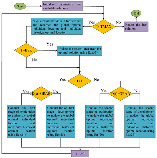
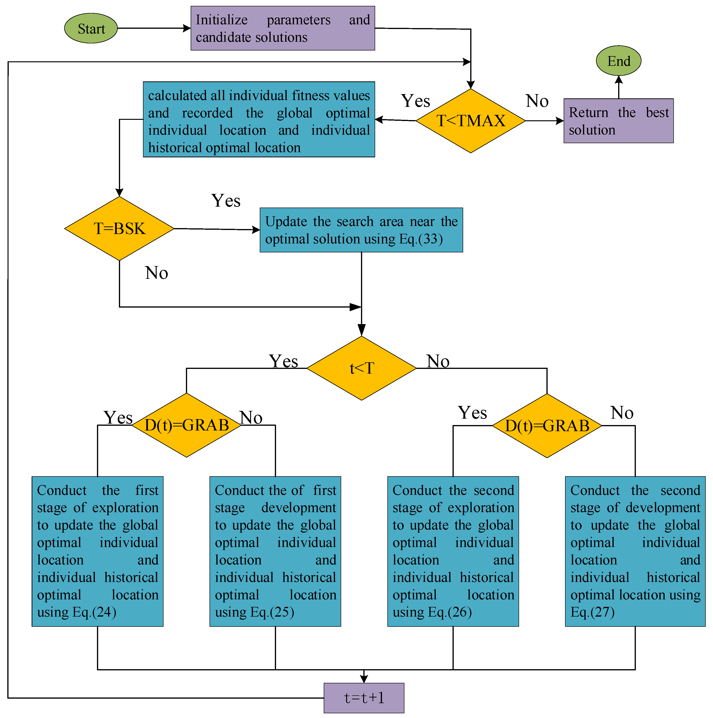
The pseudo-code of the proposed ISCHO is detailed in Table 2. The detailed flowchart of ISCHO is presented in Figure 3.

Table 2. Pseudo-code of the Improved Sinh Cosh optimizer (ISCHO).

1: Initialize ISCHO parameters

2: Initialize the positions of candidate solutions randomly.

3: According to the “first grabbing then washing “ strategy, update Equation (28) to Equation (32)

4: For t = 1:Tmax 5: Calculate the Fitness values of the candidate solutions (X). 6: Find the Optimal solution so far.

7:  If T = BSK

8:    Update the population position according to Equation (33) and update the BSK.

9:  Else If t < T

10:      If D(t) = GRAB

11:        Update the position of candidate solutions by using Equation (24)

12:       Else If D(t) = WASH

13:        Update the position of candidate solutions by using Equation (25)

14:      End

15:     Else

16:      If D(t) = GRAB

17:        Update the position of candidate solutions by using Equation (26)

18:      Else If D(t) = WASH

19:        Update the position of candidate solutions by using Equation (27)

20:      End

21:    End

22:  End

23: End

24: Output: The optimal individual position and the optimal objective function.

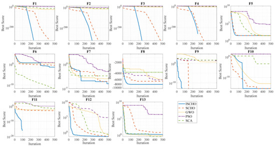
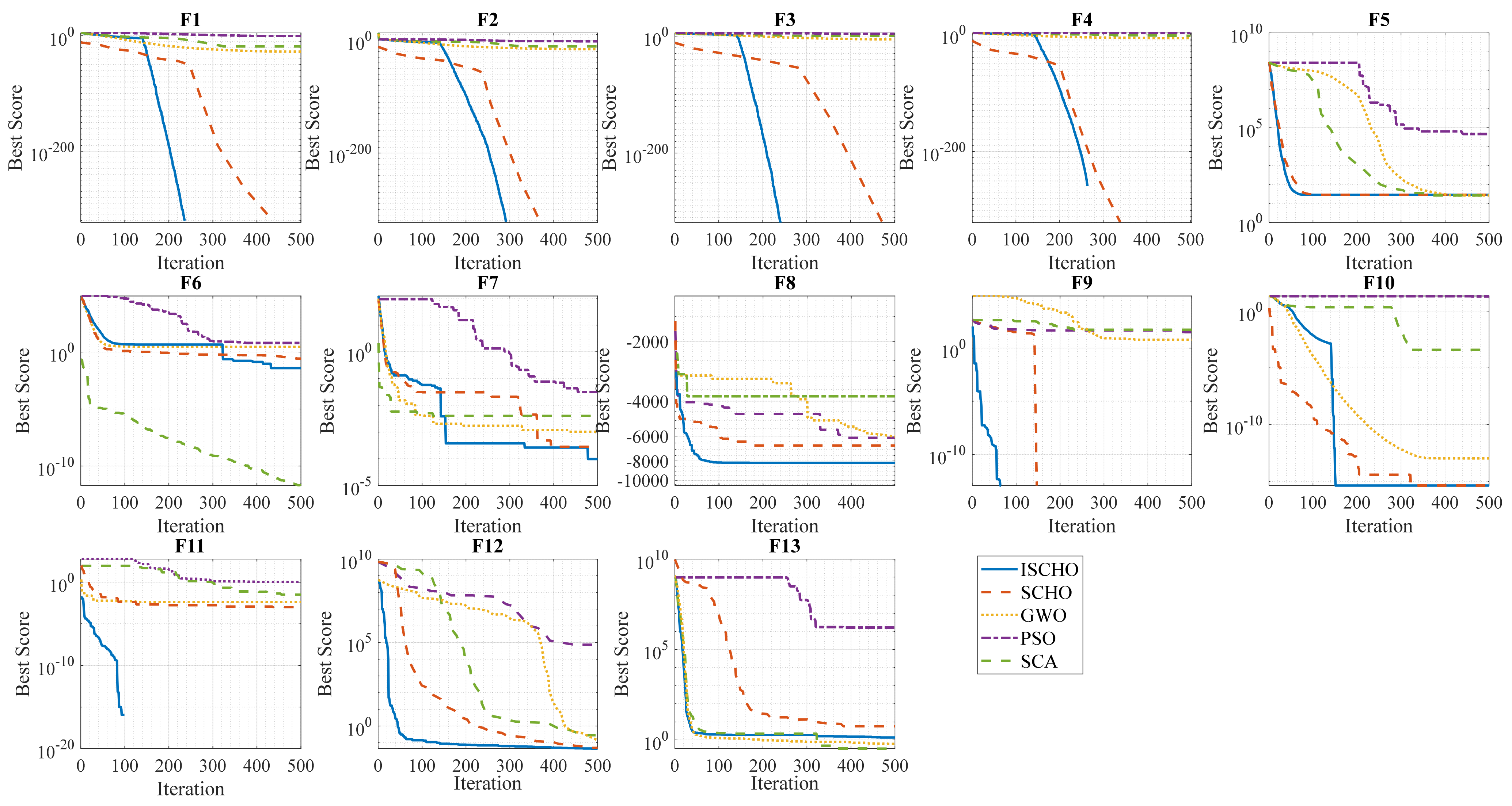
Figure 3. Convergence curves of ISCHO and comparison algorithms for 13 test benchmark functions.

The superiority of the proposed technique is tested using 13 standard single-peak and multi-peak reference functions [34]. For these tests, the number of search agents (N) and iterations (Max_interation) are specified as 30 and 500, respectively, and then these algorithms run for 15,000 fitness evaluations to find the optimal solution. Each algorithm on each tested function is run independently 30 times to ensure that optimization results are not just a random occurrence. These results obtained by ISCHO and other comparison algorithms are shown in Table 3. The convergence curves of ISCHO and other algorithms for the 13 tested functions are shown in Figure 3.

Table 3. Comparison of proposed ISCHO with other techniques for test functions.

	ISCHO		SCHO		GWO		SCA		PSO
	M × an	SD	M × an	SD	M × an	SD	M × an	SD	M × an	SD
F1	0	0	0	0	1.44 $\times$ 10−27	2.35 $\times$ 10−27	2.35 × 10−24	7.74 × 10−24	1.13 × 101	2.27 × 101
F2	0	0	0	0	8.32 × 10−17	5.35 × 10−17	9.68 × 10−11	1.27 × 10−11	2.50 × 10−2	6.31 × 10−2
F3	0	0	0	0	1.03 × 10−4	4.52 × 10−4	8.57 × 10−2	7.12 × 10−2	1.02 × 104	6.28 × 103
F4	0	0	0	0	7.62 × 10−7	6.67 × 10−7	1.00 × 10−2	9.70 × 10−3	3.40 × 101	1.23 × 101
F5	2.41 × 101	6.53 $\times$ 10−1	2.84 × 101	5.49 × 10−1	2.70 × 101	6.64 × 10−1	4.65 × 101	3.59 × 101	1.42 × 105	5.41 × 105
F6	3.67 × 10−2	1.34 × 100	2.72 × 10−1	1.25 × 100	2.13 × 100	3.40 × 10−1	1.25 × 10−12	8.18 × 10−15	6.07 × 100	3.26 × 101
F7	8.88 × 10−5	8.37 × 10−5	1.05 × 10−4	7.05 × 10−5	1.99 × 10−3	1.09 × 10−3	7.00 × 10−3	2.70 × 10−3	1.29 × 10−2	1.42 × 10−1
F8	−8.17 × 103	2.32 × 103	−6.69 × 103	2.69 × 103	−6.01 × 103	8.40 × 102	−3.76 × 103	8.38 × 102	−5.92 × 103	2.64 × 102
F9	0	0	0	0	2.84 × 100	3.46 × 100	4.44 × 101	9.86 × 100	4.08 × 101	3.47 × 101
F10	4.44 × 10−16	0	4.44 × 10−16	0	1.02 × 10−13	2.07 × 10−14	3.43 × 10−4	6.38 × 10−1	1.39 × 101	8.77 × 100
F11	0	0	1.00 × 10−3	3.66 × 10−3	2.45 × 10−3	5.66 × 10−3	1.60 × 10−2	2.20 × 10−2	9.51 × 10−1	4.13 × 10−1
F12	1.36 × 10−1	2.60 × 10−1	2.78 × 10−1	3.03 × 10−1	4.20 × 10−2	2.30 × 10−2	4.84 × 10−2	1.21 × 10−1	7.39 × 104	2.58 × 105
F13	1.34 × 100	9.47 × 10−1	5.39 × 100	8.40 × 10−1	6.01 × 10−1	2.57 × 10−1	1.14 × 10−1	1.96 × 10−1	4.63 × 105	2.23 × 106

As shown in Table 3, among the seven single-peak benchmark functions, ISCHO achieves the best performance on F1, F2, F3, F4, F5, and F7. Specifically, on F1 through F4, ISCHO attains the theoretical global optimum of zero with zero standard deviation, demonstrating not only exceptional convergence precision and numerical stability but also, as evidenced by the convergence curves of Figure 4, a faster convergence rate compared to other algorithms. For F6, although SCA yields the optimal result, ISCHO still maintains competitive optimization performance. Regarding the multi-peak functions, ISCHO exhibits excellent performance on F8, F9, F10, F11, and F12. On F13, while the final mean value achieved by ISCHO is slightly inferior to that of SCA, the difference is marginal, and ISCHO demonstrates a notably faster convergence speed, along with a substantial improvement over the original SCHO algorithm. It is worth emphasizing that ISCHO consistently outperforms the original SCHO across all 13 test functions.

Figure 4. Flowchart of ISCHO.

In summary, although ISCHO does not achieve absolute optimality on every individual test function, from an overall performance perspective, it attains optimal or tied-optimal results on 11 out of the 13 benchmark functions, significantly surpassing the original SCHO and other compared algorithms. These findings fully validate the effectiveness of the proposed “first grabbing then washing” strategy in balancing global exploration and local exploitation, thereby establishing a solid foundation for its subsequent application to load frequency control problems.

2.4. Problem Formulation

In the power system, the main objectives of load frequency control (LFC) in the presence of interference are as follows: (1) eliminate frequency vibration and reduce frequency fluctuations caused by load changes; (2) maintain the exchange power of the liaison line within the specified range to ensure that the power exchange between different areas is smooth.

In order to achieve these goals, LFC optimization problems need to define objective functions. A variety of criteria have been discussed in the literature for the accumulation of frequency deviation and tie-line power deviation. After investigation, ITAE (integral of time multiplied by absolute error) was found to be an effective standard, generally superior to other criteria such as IAE, ISE, and ISTE, as it better reflects the response of the system to frequency changes. Therefore, we used ITAE as the objective function of the test system, focusing on the frequency drift and the power increment of the contact line in each area to improve the dynamic performance of the system and reduce potential risks. In LFC, the ITAE of the frequency change in each area and the power increment change in the liaison line is taken as the following objective function:

$$J=ITAE=\sum _{i=1}^N{\int }_0^{t_{sim}}\left(\left|\Delta f_i\right|+\sum _{\begin{array}{c}j=1\\ j\ne i\end{array}}^N\left|\Delta P_{ti{e}_{i-j}}\right|\right).t.dt$$

(35)

where $\Delta f_i$ is the frequency shift in each area, $\Delta P_{ti{e}_{i-j}}$ is the incremental change in the power of the liaison line, and $t_{sim}$ is the analog period. The boundary of the controller parameters is the constraint of the problem. Therefore, design can be expressed as an optimization problem: Minimize J.

For the PID controller: $K_{p_{min}}\le K_p\le K_{p_{max}};K_{i_{min}}\le K_i\le K_{i_{max}};K_{d_{min}}\le K_d\le K_{d_{max}};$

For the PIDF-II controller: $K_{p_{min}}\le K_p\le K_{p_{max}};K_{i_{min}}\le K_i\le K_{i_{max}};K_{d_{min}}\le K_d\le K_{d_{max}};$ $N_{min}\le N\le N_{min};K_{I{I}_{min}}\le K_{II}\le K_{I{I}_{max}};$

For the 2DOF-PID controller: $K_{p_{min}}\le K_p\le K_{p_{max}};K_{i_{min}}\le K_i\le K_{i_{max}};K_{d_{min}}\le K_d\le K_{d_{max}};$ $P{w}_{min}\le Pw\le P{w}_{min};D{w}_{min}\le Dw\le D{w}_{min};$

For the 2DOF-PIDF-II controller: $K_{p_{min}}\le K_p\le K_{p_{max}};K_{i_{min}}\le K_i\le K_{i_{max}};K_{d_{min}}\le K_d\le K_{d_{max}};$ $P{w}_{min}\le Pw\le P{w}_{min};D{w}_{min}\le Dw\le D{w}_{min}; N_{min}\le N\le N_{min};K_{I{I}_{min}}\le K_{II}\le K_{I{I}_{max}}$.

3. Simulation Results and Discussion

The considered system was simulated in MATLAB. Code implementing object-oriented analysis was developed in files, which interfaced with the established model of the studied power system, and the Simulink model was reused for the optimization process. Here, the simulation results are performed on a laptop system with an Intel Core i7 CPU of 2.7 GHz, 64-bit processor. All optimizers use a population size of 30 and a maximum of 50 iterations, and then these algorithms run for 1500 fitness evaluations to find the optimal solution.

This chapter is divided into four parts: (1) We compared the proposed controller with other controllers and observed the performance of the proposed controller. (2) By adding various disturbances to the system and considering the volatility of new energy generation, we observed the performance of ISCHO and other optimization algorithms and also observed the performance of ISCHO. (3) Considering the communication delay, we observed the robustness of the proposed control method. (4) We tested the robustness of the system when its system parameters changes.

3.1. Controller Performance Test

In order to verify the performance of the 2DOF-PIDF-II controller proposed in this paper, from the literature survey, we consider some relevant controllers as a comparison to implement the proposed algorithm. These include the proportional integral derivative (PID) controller, 2DOF-PID controller and PIDF-II controller.

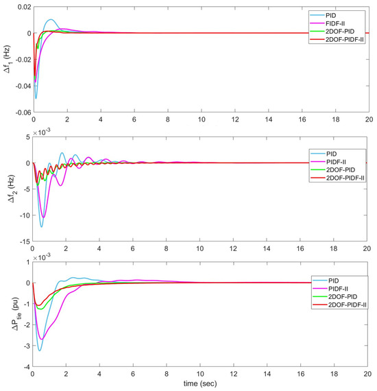
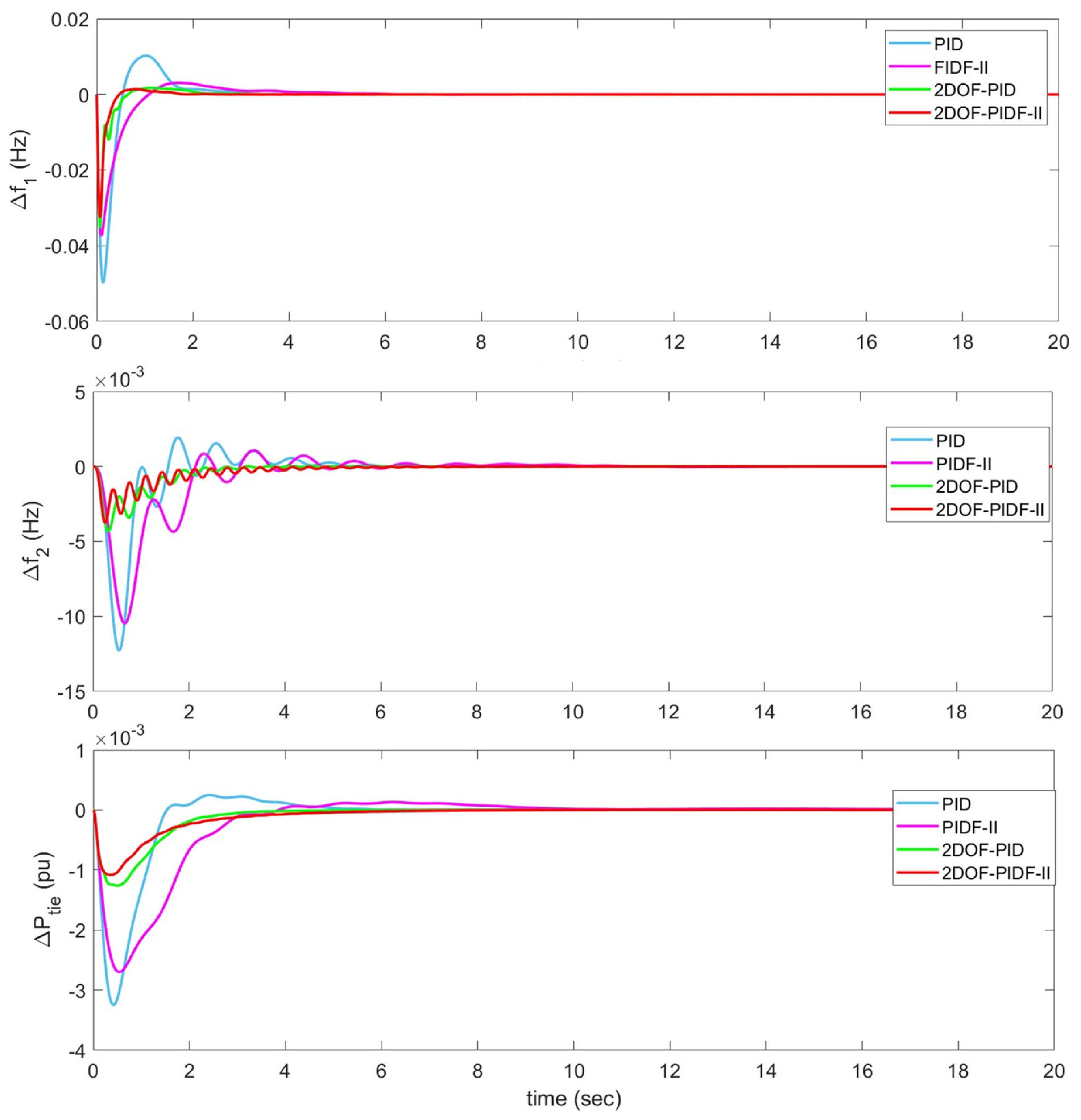
The proposed 2DOF-PIDF-II controller is compared with other controllers by adding a step load disturbance of 0.1 P.U. to area 1 at time t = 0. Figure 5 shows the frequency deviation and tie-line power for each area of the different controllers, and Table 4 shows the LFC performance parameters for these controllers. It can be seen from Figure 5 and Table 2 that the 2DOF-PIDF-II controller has the optimal maximum overshoot and minimum undershoot in all performance indexes of LFC. ΔF1 and ΔF2 have the shortest stability time and the smallest objective function value, which is better than the other three controllers.

Figure 5. Transient responses for different controllers.

Table 4. LFC performance parameters of different controllers.

		ST	MU	MO	JITA × 10
ΔF1	PID	3.8146	−0.4976	0.01024	0.030698
	PIDF-II	6.1681	−0.3741	0.00309	0.049535
	2DOF-PID	3.8657	−0.0354	0.0017	0.010726
	2DOF-PIDF-II	2.4003	−0.0326	0.0014	0.010391
ΔF2	PID	6.9139	−0.01227	0.001922	—
	PIDF-II	10.8235	−0.01047	0.001082	—
	2DOF-PID	5.9175	−0.00432	2.09 × 10−5	—
	2DOF-PIDF-II	5.4159	−0.00377	4.31 × 10−6	—
ΔPTIE	PID	4.748	−0.00325	0.000246	—
	PIDF-II	8.6885	−0.0027	0.000129	—
	2DOF-PID	4.0057	−0.00126	1.95 × 10−6	—
	2DOF-PIDF-II	3.6221	−0.00108	1.69 × 10−6	—

3.2. Test of ISCHO

In the above summary, we have verified the effectiveness of the 2DOF-PIDF-II controller. In the following experiments, we will verify the effectiveness of ISCHO in the field of LFC under different loads by comparing it with various algorithms.

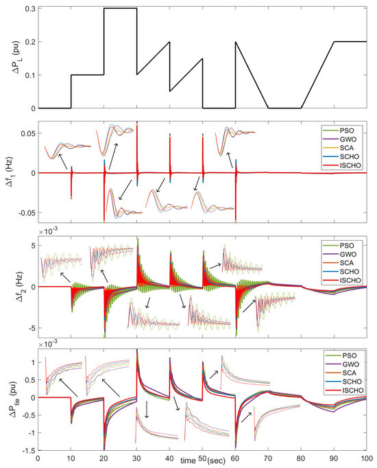
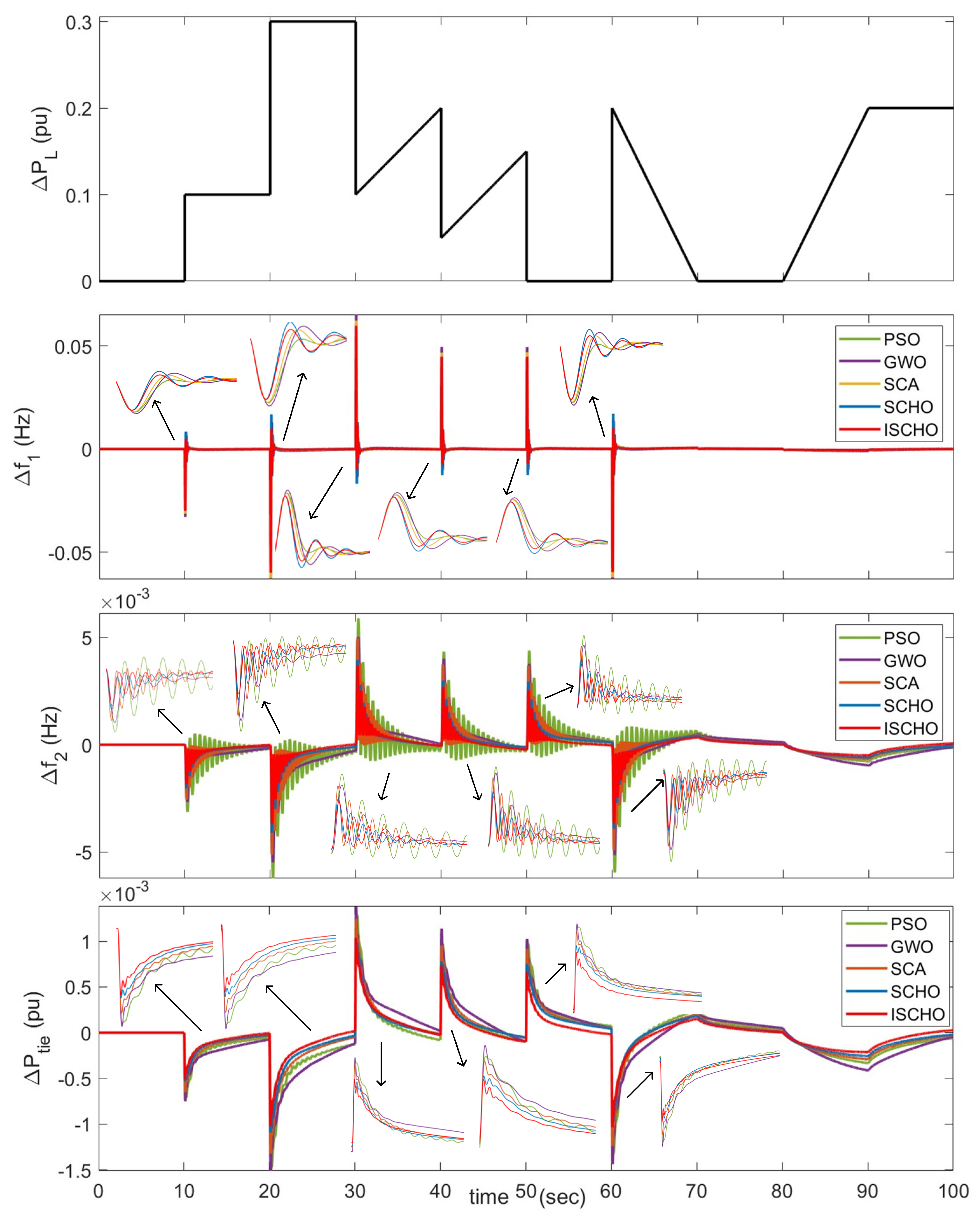
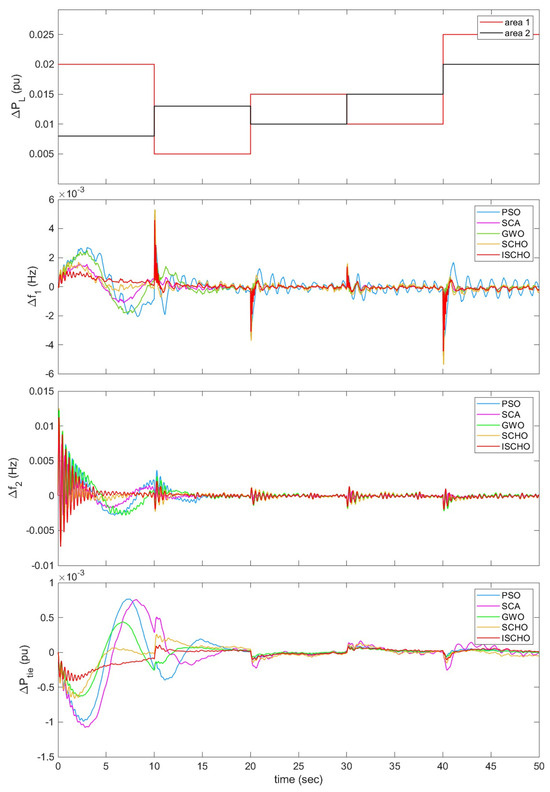
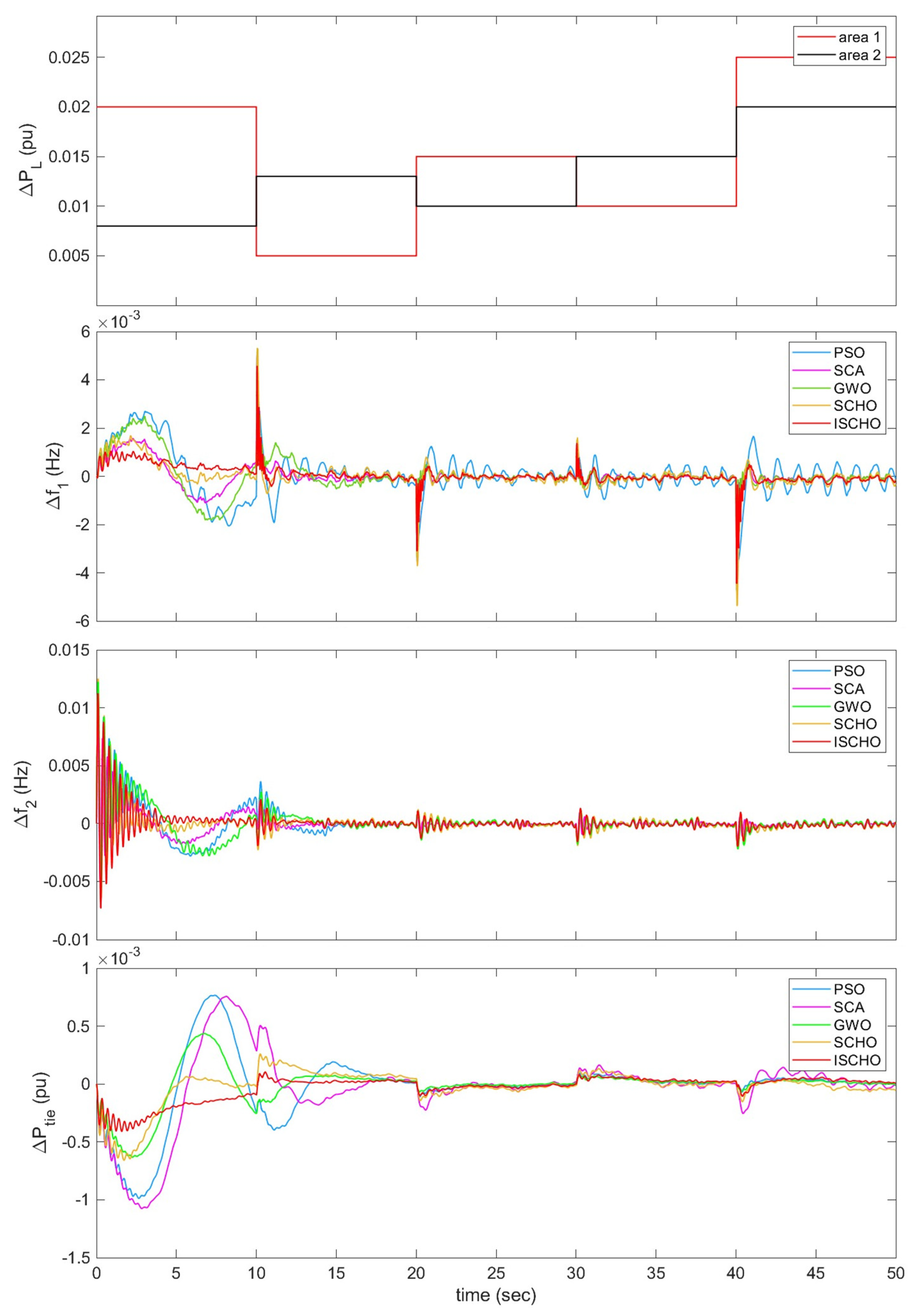
In this section, we apply the following three different types of disturbances to the system. Disturbance 1: At t = 0, add a step load perturbation (SLP) to area 1. Disturbance 2: Add a random load perturbation (RLP) to area 1. Disturbance 3: While increasing the random fluctuations of new energy generation, add multiple step load perturbation (MSLP) to area 1 and area 2.

Figure 6 shows the frequency deviation and tie-line power for each area where different optimization algorithms have been applied, and Table 5 shows the LFC performance parameters for these optimizers.

Figure 6. Transient responses of different optimizers in the case of disturbance 1.

Table 5. The parameter performance of different optimizers in the case of disturbance 1.

		ST	MU	MO	JITA × 10
ΔF1	PSO	3.7833	−0.04834	0.003679	0.018109
	GWO	3.38049	−0.04735	0.008694	0.016808
	SCA	4.72967	−0.03682	0.00139	0.015521
	SCHO	2.81062	−0.03794	0.001969	0.011408
	ISCHO	1.75614	−0.02979	0.001875	0.0066953
ΔF2	PSO	5.48871	−0.007276	7.859 × 10−4	—
	GWO	3.67	−0.004884	6.435 × 10−6	—
	SCA	3.26	−0.003579	4.27 × 10−5	—
	SCHO	2.71	−0.004717	2.616 × 10−6	—
	ISCHO	1.92	−0.004323	6.042 × 10−7	—
ΔPTIE	PSO	6.50	−0.002468	1.393 × 10−4	—
	GWO	3.49	−0.001284	4.105 × 10−6	—
	SCA	2.05588	−0.001394	1.371 × 10−5	—
	SCHO	2.50408	−0.00138	8.221 × 10−7	—
	ISCHO	1.92351	−0.00116	3.634 × 10−7	—

For the frequency deviation response (ΔF1) of area 1, compared with the PSO, GWO, SCA and SCHO, the ISCHO controller reduced the maximum deviation by 38.37%, 37.08%, 19.09% and 21.48%, respectively, and the settling time was reduced by 2.03 s, 1.62 s, 2.97 s and 1.05 s, respectively. For the frequency deviation response (ΔF2) of area 2, the maximum deviation was reduced by 40.59% and 11.49% and increased by 20.77% and 8.35%, respectively. The settling time was reduced by 3.57 s, 1.75 s, 1.34 s, and 0.79 s, respectively. For the power deviation response of the tie line (ΔPTIE), the maximum deviation was reduced by 53.00%, 9.66%, 16.79%, and 15.94%, respectively, and the settling time was reduced by 4.58 s, 1.57 s, 0.13 s, and 0.58 s, respectively.

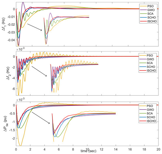
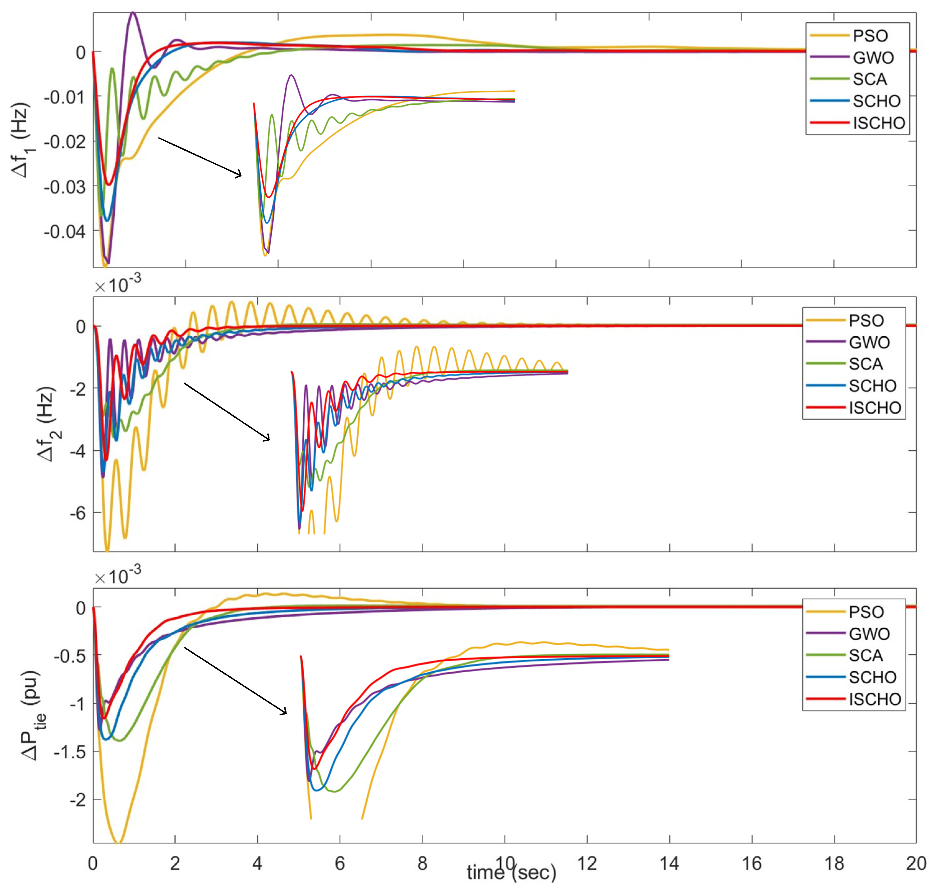
Figure 7 shows the frequency deviation and contact line power of each area where different optimization algorithms are applied, and Table 6 shows the LFC performance parameters of different optimization algorithms.

Figure 7. Transient responses of different optimizers in the case of disturbance 2.

Table 6. The parameter performance of different optimizers in the case of disturbance 2.

		STD	MU	MO	JITA × 10
ΔF1	PSO	0.004156	−0.06313	0.0627	6.9554
	GWO	0.004242	−0.06598	0.06576	5.7306
	SCA	0.003859	−0.06255	0.06225	6.2597
	SCHO	0.003364	−0.05958	0.05948	4.3652
	ISCHO	0.003144	−0.05493	0.05627	3.6434
ΔF2	PSO	9.276 × 10−4	−0.006216	0.005895	—
	GWO	8.186 × 10−4	−0.005483	−0.005483	—
	SCA	7.028 × 10−4	−0.005137	0.004961	—
	SCHO	5.668 × 10−4	−0.004109	0.003955	—
	ISCHO	5.112 × 10−4	−0.003689	0.003696	—
ΔPTIE	PSO	3.125 × 10−4	−0.00151	0.001329	—
	GWO	3.175 × 10−4	−0.001569	0.001376	—
	SCA	2.673 × 10−4	−0.001322	0.001243	—
	SCHO	2.232 × 10−4	−0.001193	0.001181	—
	ISCHO	1.862 × 10−4	−0.001033	0.001036	—

For the frequency deviation response (ΔF1) of area 1, compared with the PSO, GWO, SCA and SCHO controllers, the ISCHO controller reduced the maximum deviation by 12.99%, 16.75%, 12.18% and 7.80%, respectively, and the standard deviation decreased by 24.35%, 25.89%, 18.54% and 6.54%, respectively. For the frequency deviation response (ΔF2) of area 2, the maximum deviation was reduced by 40.65%, 32.73%, 28.18%, and 10.22%, respectively, and the standard deviation was reduced by 44.88%, 37.55%, 27.25%, and 9.81%, respectively. For the power deviation response of the tie line (ΔP_TIE), the maximum deviation was reduced by 31.59%, 34.16%, 21.87%, and 13.40%, respectively, and the standard deviation was reduced by 40.38%, 41.35%, 30.33%, and 16.58%, respectively.

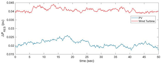
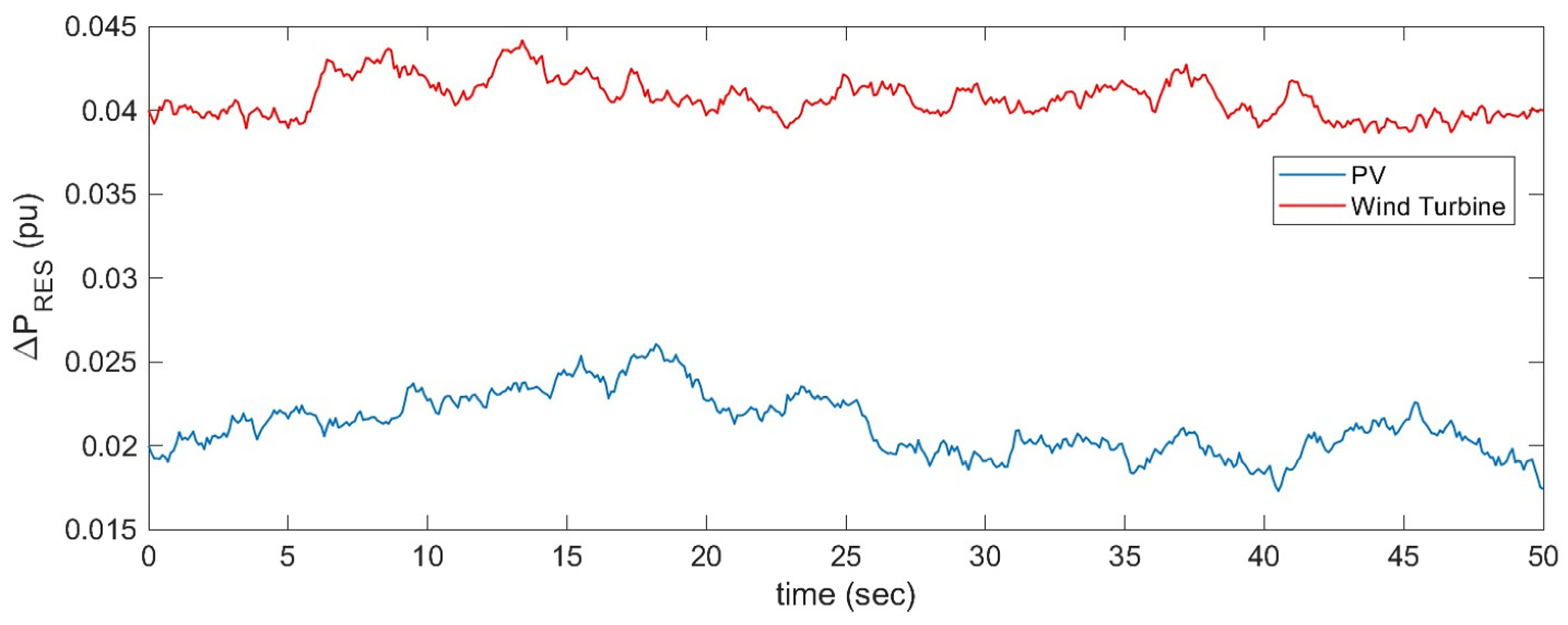
Figure 8 shows the frequency deviation and contact line power of each area where different optimization algorithms are applied, and Table 7 shows the LFC performance parameters of different optimization algorithms. Meanwhile, we took into account the fluctuation patterns of solar power generation and wind power generation as shown in Figure 9. For the frequency deviation response (ΔF1) of area 1, compared with the PSO, SCA, GWO and SCHO controllers, the maximum deviation of the ISCHO controller was reduced by 12.71%, 8.56%, 11.09% and 3.19%, respectively, and the standard deviation was reduced by 13.80%, 14.76%, 17.52% and 6.71%, respectively. For the frequency deviation response (ΔF2) of area 2, the maximum deviation was reduced by 43.08%, 28.85%, 27.45%, and 9.76%, respectively, and the standard deviation was reduced by 47.06%, 27.21%, 35.21%, and 6.43%, respectively. For the power deviation response of the tie line (ΔPTIE), the maximum deviation was reduced by 29.41%, 7.69%, 14.29%, and 0.00%, respectively, and the standard deviation was reduced by 99.94%, 20.25%, 36.79%, and 10.43%, respectively.

Figure 8. Transient responses of different optimizers in the case of disturbance 3.

Table 7. The parameter performance of different optimizers in the case of disturbance 3.

		STD	MU	MO	JITA × 10
ΔF1	PSO	0.000355	−0.00661	0.006036	0.64554
	SCA	0.000359	−0.00631	0.006301	0.47306
	GWO	0.000371	−0.00649	0.006451	0.62597
	SCHO	0.000328	−0.00596	0.006095	0.42794
	ISCHO	0.000306	−0.00577	0.005879	0.36476
ΔF2	PSO	9.35 × 10−5	−0.00065	0.00062	—
	SCA	6.80 × 10−5	−0.00052	4.98 × 10−4	—
	GWO	7.64 × 10−5	−0.00051	4.73 × 10−4	—
	SCHO	5.29 × 10−5	−0.00041	3.54 × 10−4	—
	ISCHO	4.95 × 10−5	−0.00037	3.38 × 10−4	—
ΔPTIE	PSO	3.29 × 10−2	−0.00017	1.52 × 10−4	—
	SCA	2.37 × 10−5	−0.00013	1.24 × 10−4	—
	GWO	2.99 × 10−5	−0.00014	1.24 × 10−4	—
	SCHO	2.11 × 10−5	−0.00012	1.20 × 10−4	—
	ISCHO	1.89 × 10−5	−0.00012	1.04 × 10−4	—

Figure 9. Renewable energy disturbance.

From the above performance, it can be seen that the ISCHO demonstrates comprehensive advantages in load frequency control. It can achieve the shortest or nearly shortest settling time in all disturbances, significantly accelerating the system recovery speed. At the same time, this controller can minimize the maximum dynamic deviations of frequency and line power, enhancing transient stability. Moreover, ISCHO has the lowest standard deviation and performance indicators, proving that its response consistency and comprehensive control performance are the best.

3.3. The Test of the Time-Delay Robustness of the Proposed Control Method

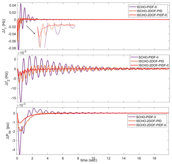
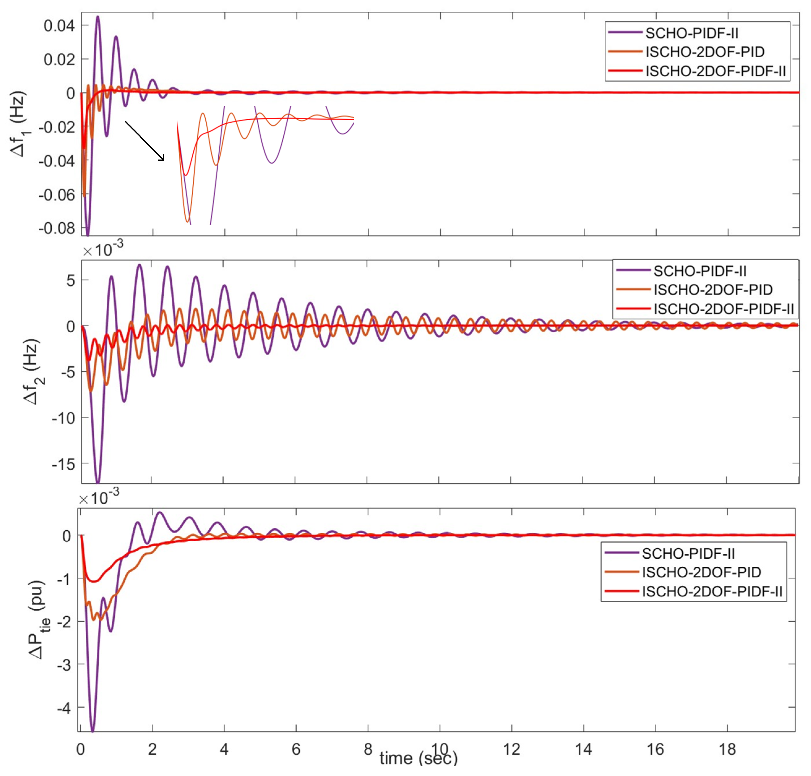
The traditional LFC system uses dedicated lines to transmit signals, and this transmission method is fast with negligible communication delay. However, when information is transmitted through a communication network, the control signals are prone to significant delay during transmission. Therefore, analyzing the robustness of the controller under communication delay is a very necessary task. Taking the second interference scenario described in the previous text as an example, this section analyzes the robust performance of the designed ISCHO-2DOF-PIDF-II, ISCHO-2DOF-PID, and SCHO-PIDF-II controllers when the system is affected by 100 ms communication delays.

According to the simulation results shown in Figure 10, the existence of communication delay will prolong the time for the system to stabilize. Although the adjustment time becomes longer, the ISCHO-2DOF-PIDF-II controllers designed in this paper can all achieve the load frequency control of the system, further verifying that the designed controller has good control performance and robustness.

Figure 10. The system responses under a 100 ms communication delay.

3.4. Robustness Analysis Considering Changes in System Parameters

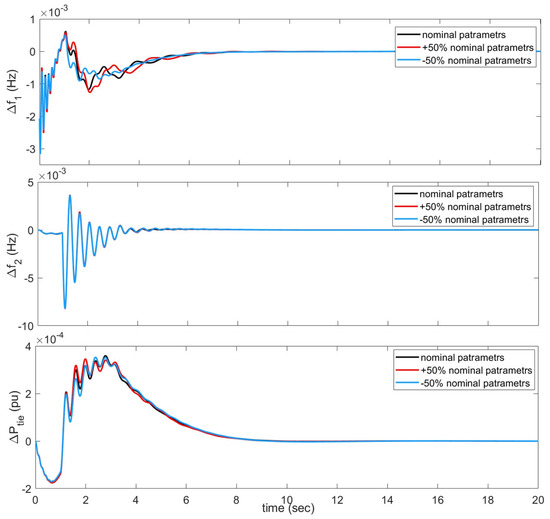
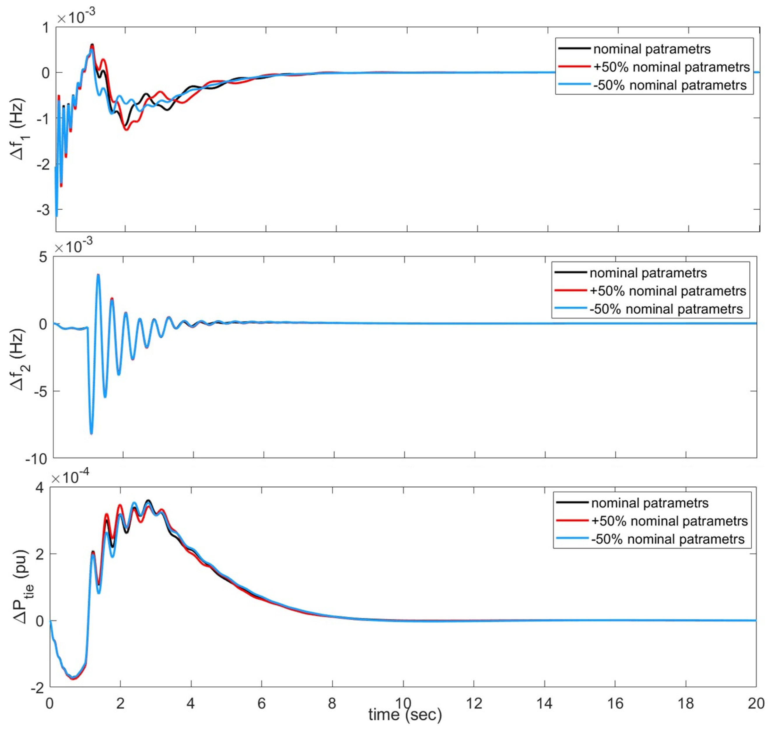
In this scenario, the performance of 2DOF-PIDF-II is studied when the system parameters Tsg, Tt, Tgh, Xg and Yg vary by ±50%. At the same time, step load perturbations are applied to areas 1 and 2 and selected as 0.01 P.U. and 0.03 P.U.

Figure 11 shows the frequency deviation of the two areas and the power change in the tie line after the system parameter changes by ±50%. It can be inferred from Figure 10 that the ±50% change in system parameters and the step load perturbations applied to areas 1 and 2 do not have much effect on the performance of the 2DOF-PIDF-II controller.

Figure 11. The system responses based on a ±50% change in the system parameters.

4. Conclusions and Future Work

This study presents an improved Sinh and Cosh optimizer optimized two-degree-of-freedom double integral feedback PID (ISCHO-2DOF-PIDF-II) controller for load frequency regulation in a two-area power system integrating four generation sources: reheat thermal, hydro, wind, and photovoltaic plants. The proposed approach undergoes rigorous validation through three critical phases: Initially, ISCHO demonstrates superior optimization capabilities against established algorithms (PSO, SCA, GWO, SCHO) across 13 text functions. Subsequently, under nonlinear generation constraints including Governor Dead Band and Generation Rate constraints, the controller exhibits exceptional disturbance rejection across diverse load scenarios, outperforming comparative control strategies. Furthermore, when subjected to system parameter uncertainties and communication delays, the ISCHO-2DOF-PIDF-II maintains robust stability and performance integrity. Collectively, these results confirm the ISCHO-2DOF-PIDF-II as an effective solution for frequency stabilization in complex multi-source power systems, demonstrating enhanced optimization efficacy, superior transient performance under practical constraints, and reliable operation amid modeling uncertainties.

It is important to note that the current study primarily validates the proposed method on a two-area nonlinear system, and comprehensive testing on larger-scale multi-area systems has not yet been conducted. Furthermore, we acknowledge that the theoretical analysis of the ISCHO algorithm in this study remains limited, which will be a focal point of our future research. Consequently, future work will concentrate on the following aspects: (1) Conducting a more rigorous mathematical analysis of the ISCHO algorithm, including its computational complexity and parameter adaptation mechanisms, to establish a stronger theoretical foundation for its application to more complex engineering problems. (2) Applying the proposed control method to three-area and larger interconnected systems to validate its scalability and applicability in more complex topological configurations. (3) Introducing more realistic nonlinear characteristics and communication network constraints, such as time-varying delays and data dropouts, into the system model to rigorously assess the controller’s robustness in practical complex environments. (4) Modeling energy storage systems (ESS) in conjunction with renewable generation sources (wind and PV) and applying the proposed optimization method for coordinated control of such hybrid systems. This aims to mitigate the intermittency of renewables and improve the overall flexibility and stability of the power system.

References

- Wadi, M.; Shobole, A.; Elmasry, W.; Kucuk, I. Load frequency control in smart grids: A review of recent developments. Renew. Sustain. Energy Rev. 2024, 189, 114013. [Google Scholar] [CrossRef] [Scilit]
- Gulzar, M.M.; Sibtain, D.; Alqahtani, M.; Alismail, F.; Khalid, M. Load frequency control progress: A comprehensive review on recent development and challenges of modern power systems. Energy Strat. Rev. 2025, 57, 101604. [Google Scholar] [CrossRef] [Scilit]
- Zhang, Q.; Zou, K.; Zhang, Z. An imprved Sinh Cosh optimizer based 2-degree-of-freedom double integral feedback PID controller for power system load frequency control. Authorea Prepr 2025. [Google Scholar] [CrossRef] [Scilit]
- Ojaghi, P.; Rahmani, M. LMI-based robust predictive load frequency control for power systems with communication delays. IEEE Trans. Power Syst. 2017, 32, 4091–4100. [Google Scholar] [CrossRef] [Scilit]
- Rahmani, M.; Sadati, N. Hierarchical optimal robust load-frequency control for power systems. IET Gener. Transm. Distrib. 2012, 6, 303–312. [Google Scholar] [CrossRef] [Scilit]
- Xiahou, K.S.; Liu, Y.; Wu, Q.H. Robust load frequency control of power systems against random time-delay attacks. IEEE Trans. Smart Grid 2020, 12, 909–911. [Google Scholar] [CrossRef] [Scilit]
- Wang, P.; Guo, J.; Cheng, F.; Gu, Y.; Yuan, F.; Zhang, F. A MPC-based load frequency control considering wind power intelligent forecasting. Renew. Energy 2025, 244, 122636. [Google Scholar] [CrossRef] [Scilit]
- Zhou, J.; Jia, Y.; Yong, P.; Liu, Z.; Sun, C. Robust deep Koopman model predictive load frequency control of interconnected power systems. Electr. Power Syst. Res. 2024, 226, 109948. [Google Scholar] [CrossRef] [Scilit]
- Gbadega, P.A.; Saha, A.K. Load frequency control of a two-area power system with a stand-alone microgrid based on adaptive model predictive control. IEEE J. Emerg. Sel. Top. Power Electron. 2020, 9, 7253–7263. [Google Scholar] [CrossRef] [Scilit]
- Tran, A.T.; Van Huynh, V.; Nguyen, B.L.H.; Shim, J.W.; Do, T.D. Multi-stage sliding mode control design with optimal state estimator for load frequency regulation in hybrid-source power systems. Sci. Rep. 2025, 15, 43795. [Google Scholar] [CrossRef] [Scilit]
- Elsisi, M.; Baz Mohammadi, N.; Guerrero, J.M.; Ebrahim, M.A. Energy management of controllable loads in multi-area power systems with wind power penetration based on new supervisor fuzzy nonlinear sliding mode control. Energy 2021, 221, 119867. [Google Scholar] [CrossRef] [Scilit]
- Patel, A.; Purwar, S. Design of event trigger based multirate sliding mode load frequency controller for interconnected power system. ISA Trans. 2023, 137, 457–470. [Google Scholar] [CrossRef] [Scilit]
- Tuan, D.H.; Tran, D.T.; Nguyen Ngoc Thanh, V.; Huynh, V.V. Load Frequency Control Based on Gray Wolf Optimizer Algorithm for Modern Power Systems. Energies 2025, 18, 815. [Google Scholar] [CrossRef] [Scilit]
- Hasan, R.; Hasan, M.; Rana, M.S.; Tabassum, F.; Reza, M.N.B. Disturbance Observer-Aided SSA-TID Control for Frequency Stabilisation in Hybrid Renewable Power Systems. IET Renew. Power Gener. 2025, 19, e70137. [Google Scholar] [CrossRef] [Scilit]
- Shouran, M.; Alsseid, A.M. Cascade of fractional order PID based PSO algorithm for LFC in two-area power system. In Proceedings of the 2021 3rd International Conference on Electronics Representation and Algorithm (ICERA), Liverpool, UK, 4–6 July 2021; pp. 1–6. [Google Scholar]
- Boonkirdram, S.; Audomsi, S.; Sa-Ngiamvibool, W.; Kasemsin, W. Design of Two-Degree-of-Freedom PID Controllers Optimized by Bee Algorithm for Frequency Control in Renewable Energy Systems. Energies 2025, 18, 4880. [Google Scholar] [CrossRef] [Scilit]
- Gupta, N.K.; Kar, M.K.; Singh, A.K. Design of a 2-DOF-PID controller using an improved sine-cosine algorithm for load frequency control of a three-area system with nonlinearities. Prot. Control Mod. Power Syst. 2022, 7, 33. [Google Scholar] [CrossRef] [Scilit]
- Dhanasekaran, B.; Kaliannan, J.; Baskaran, A.; Dey, N.; Tavares, J.M.R.S. Load frequency control assessment of a PSO-PID controller for a standalone multi-source power system. Technologies 2023, 11, 22. [Google Scholar] [CrossRef] [Scilit]
- Semwal, S.; Mittal, A.; Kumar, S.; Goyal, S.; Singh, A. Comparative analysis of two-area load frequency control using tilted-integral-derivative (TID) and proportional-integral-derivative (PID) controllers. In Proceedings of the 2024 1st International Conference on Trends in Engineering Systems and Technologies (ICTEST), Hyderabad, India, 18–19 January 2024; pp. 1–5. [Google Scholar]
- Amiri, F.; Eskandari, M.; Moradi, M.H. Improved load frequency control in power systems hosting wind turbines by an augmented fractional order PID controller optimized by the powerful owl search algorithm. Algorithms 2023, 16, 539. [Google Scholar] [CrossRef] [Scilit]
- Amarendra, K.; Teeparthi, K.; Vamsi, Y.R.; Veeramsetty, V.; Thota, V.V.N.P. Load frequency control of an interconnected microgrid using MGO-based 2DOF-PID Controller. In Proceedings of the 2023 7th International Conference on Computer Applications in Electrical Engineering-Recent Advances (CERA), Roorkee, India, 10–12 August 2023; pp. 1–6. [Google Scholar]
- Hussain, J.; Zou, R.; Pathak, P.K.; Karni, A.; Akhtar, S. Design of a novel cascade PI-(1+ FOPID) controller to enhance load frequency control performance in diverse electric power systems. Electr. Power Syst. Res. 2025, 243, 111488. [Google Scholar] [CrossRef] [Scilit]
- Fathy, A.; Bouaouda, A.; Hashim, F.A. A novel modified cheetah optimizer for designing fractional-order PID-LFC placed in multi-interconnected system with renewable generation units. Sustain. Comput. Inform. Syst. 2024, 101011. [Google Scholar] [CrossRef] [Scilit]
- Hussain, J.; Zou, R.; Akhtar, S.; Abouda, K.A. Design of cascade PP-FOPID controller based on marine predators algorithm for load frequency control of electric power systems. Electr. Eng. 2025, 107, 809–827. [Google Scholar] [CrossRef] [Scilit]
- Yogendra, A. AGC of two-area electric power systems using optimized fuzzy PID with filter plus double integral controller. J. Frankl. Inst. 2018, 355, 4583–4617. [Google Scholar] [CrossRef] [Scilit]
- Shahi, M.N.S.; Orka, N.A.; Ahmed, A. 2DOF-PID-TD: A new hybrid control approach of load frequency control in an interconnected thermal-hydro power system. Heliyon 2024, 10, e36753. [Google Scholar] [CrossRef] [Scilit]
- Zeidan, M.A.; Hammad, M.R.; Megahed, A.I.; AboRas, K.M.; Alkuhayli, A.; Gowtham, N. Enhancement of a hybrid electric shipboard microgrid’s frequency stability with triangulation topology aggregation optimizer-based 3DOF-PID-TI controller. IEEE Access 2024, 12, 66625–66645. [Google Scholar] [CrossRef] [Scilit]
- Khatanga, R.K.; Kumar, A.; Panda, S. A novel sine augmented scaled sine cosine algorithm for frequency control issues of a hybrid distributed two-area power system. Neural Comput. Appl. 2021, 33, 12791–12804. [Google Scholar] [CrossRef] [Scilit]
- Ojha, S.K.; Maddela, C.O. A FOPIDN-(1+ PIDN) controller design and optimization for load frequency control system integrated with renewables and electric vehicles. Electr. Eng. 2025, 107, 7617–7643. [Google Scholar] [CrossRef] [Scilit]
- Sondhi, S.; Hote, Y.V. Fractional order PID controller for perturbed load frequency control using Kharitonov’s theorem. Int. J. Electr. Power Energy Syst. 2016, 78, 884–896. [Google Scholar] [CrossRef] [Scilit]
- Sharma, M.; Prakash, S.; Saxena, S.; Dhundhara, S. Optimal fractional-order tilted-integral-derivative controller for frequency stabilization in hybrid power system using salp swarm algorithm. Electr. Power Compon. Syst. 2021, 48, 1912–1931. [Google Scholar] [CrossRef] [Scilit]
- Patel, N.C.; Debnath, M.K.; Bagarty, D.P.; Das, P. GWO tuned multi degree of freedom PID controller for load frequency control. Int. J. Eng. Technol. 2018, 7, 548. [Google Scholar] [CrossRef] [Scilit]
- Daraz, A.; Malik, S.A.; Basit, A.; Aslam, S.; Zhang, G. Modified FOPID controller for frequency regulation of a hybrid interconnected system of conventional and renewable energy sources. Fractal Fract. 2023, 7, 89. [Google Scholar] [CrossRef] [Scilit]
- Shawqran, A.M.; Attia, M.A.; Mekhamer, S.F.; Kotb, H.; Ibrahim, M.A.; Mordi, A. Enhancing Load Frequency Control in Power Systems Using Hybrid PIDA Controllers Optimized with TLBO-TS and TLBO-EDO Techniques. Processes 2025, 13, 1532. [Google Scholar] [CrossRef] [Scilit]
- Bai, J.; Li, Y.; Zheng, M.; Khatir, S.; Benaissa, B.; Abualigah, L.; Wahab, M.A. A sinh cosh optimizer. Knowl. Based Syst. 2023, 282, 111081. [Google Scholar] [CrossRef] [Scilit]
- Arya, Y.; Ahmad, R.; Nasiruddin, I.; Ahmer, M.F. LFC performance advancement of two-area RES penetrated multi-source power system utilizing CES and a new CFOTID controller. J. Energy Storage 2024, 87, 111366. [Google Scholar] [CrossRef] [Scilit]
Disclaimer/Publisher’s Note: The statements, opinions and data contained in all publications are solely those of the individual author(s) and contributor(s) and not of MDPI and/or the editor(s). MDPI and/or the editor(s) disclaim responsibility for any injury to people or property resulting from any ideas, methods, instructions or products referred to in the content. |
© 2026 by the authors. Licensee MDPI, Basel, Switzerland. This article is an open access article distributed under the terms and conditions of the Creative Commons Attribution (CC BY) license.