Multi-Strategy Collaborative Improvement of an H5N1 Viral-Inspired Optimization Algorithm for Mobile Robot Path Planning

Abstract

Mobile robots play an important role in promoting industrial intelligence and modernization. However, the existing obstacle avoidance path planning algorithms for mobile robots have poor stability and applicability. To this end, this paper proposes a path planning scheme for mobile robots based on ISH5N1 algorithm. Firstly, aiming at the problem of low initial population quality of SH5N1 algorithm, Tent chaos initialization strategy was proposed, which increased the diversity of the population, improved the quality of initial solution, and laid a foundation for subsequent deeper search. Secondly, by fusing the multi-source direction vectors and applying them to the position update, the solution accuracy of the algorithm was improved and the convergence speed of the algorithm was accelerated. Then, the mutation step size control strategy enhanced by Logistic chaos was used to enhance the ability of the algorithm to jump out of local optimum. Finally, the attenuation coefficient of inertia weight is optimized by combining cosine annealing strategy, which strengthens the ability of the algorithm to balance global search and local development. The ISH5N1 algorithm was compared with several commonly used intelligent optimization algorithms on benchmark functions and grid maps with different complexities. The results show that ISH5N1 algorithm shows good stability, higher solution accuracy and faster convergence speed in solving most benchmark functions. In the path planning experiment, the ISH5N1 algorithm can plan a shorter and smoother path, which further proves that the algorithm has good optimization ability and robustness. Finally, ablation experiments were carried out on a 20 × 20 grid map to verify the effectiveness of each optimization strategy.

1. Introduction

Autonomous mobile robot technology plays an important role in ensuring operational safety, improving task execution efficiency, reducing the risk of human error, and realizing environmentally friendly operations [1]. It is also of great significance in promoting the intelligent transformation of manufacturing and industrial logistics [2], medical and public health [3], agriculture [4], energy infrastructure [5], emergency security and rescue [6], urban management [7] and other fields. With the rapid development of mobile robot technology, the demand for robots to navigate efficiently and safely in complex environments has been increasing day by day. Path planning, as one of the key technologies for robot navigation, has received considerable attention [8]. Its function is to determine the optimal path from the starting point to the destination while avoiding obstacles [9]. At present, various algorithms have been developed in the field of mobile robot path planning [10]. According to the characteristics of these algorithms, they can be classified into four categories: traditional path planning algorithms [11,12,13], sampling-based algorithms [14,15,16], learning-based planning algorithms [17,18,19], and intelligent optimization algorithms [20,21,22]. Among them, most of the intelligent optimization algorithms are inspired by the behaviors of biological groups in nature, and they have the characteristics of simplicity, efficiency, and ease of implementation [23]. After converting the robot path planning problem into an optimization problem, these algorithms use intelligent optimization algorithms to solve the optimization problem and obtain the path planning results. Due to their relatively better performance in terms of computational efficiency and planning results, they have attracted increasing attention from researchers in recent years.

Over the past few years, many scholars have proposed path planning solutions for mobile robots based on intelligent optimization algorithms, for instance, T. Zhou et al. [24] improved the traditional ant colony algorithm for mobile robot path planning to avoid local optima, reduce blind initial searching, speed up convergence, and produce smoother paths. They modified the initial pheromone distribution, used an adaptive evaporation factor, redesigned the pheromone update rule, and added a reward–punishment mechanism. Experiments showed faster convergence and better paths, but slightly longer runtime than the original algorithm. T.-S. Lou et al. [25] proposed a hybrid Golden Jackal Wolf Optimization method for mobile robot path planning to improve convergence accuracy and reduce getting trapped in local optima. The hybrid strategy balances global and local search. Experiments showed shorter average path lengths, but the computational cost still needs improvement. T. Feng et al. [26] proposed an improved hybrid adaptive genetic algorithm for mobile robot path planning in complex environments. They pre-optimized the initial path with a domain-knowledge operator to remove redundant segments, then used a hierarchical strategy: an adaptive 2-opt operator for local refinement and improved crossover/mutation (via an S-shaped function and TANH-based AGA) to strengthen global and local search. Experiments showed better path quality, stability, and robustness, but convergence speed can still be improved. A. Loganathan et al. [27] proposed a hybrid algorithm, HHO-AVOA, for path planning that combines Harris Hawks Optimization (HHO) and African Vulture Optimization Algorithm (AVOA) to better balance global exploration and local exploitation. Experiments showed fast convergence, low computational complexity, and suitability for real-time planning. However, it has only been tested on simple maps; in more complex environments, it may get trapped in local suboptimal paths, so its robustness and adaptability still need further validation. Z. Wang et al. [28] proposed an improved Crown-Pig Optimization (CPO) algorithm for mobile robot path planning to reduce slow exploration, many iterations, and long runtime in complex environments. They used Tent chaotic mapping for population initialization and applied population reduction to speed up convergence. Experiments showed much higher search efficiency than the original CPO, but only a small improvement in path length. In addition, the algorithm’s stability was not fully validated due to limited repeated experiments.

Recent studies indicate that intelligent optimization algorithms are widely used in mobile robot path planning and can effectively improve path quality. However, existing methods still suffer from issues such as limited solution accuracy, slow convergence, long runtime, and unstable results, making it hard to balance multiple performance metrics at the same time [29]. Moreover, as mobile robots are deployed in more industries and real-world environments become more complex, algorithms must handle larger search spaces. This often leads to reduced population diversity and weak global exploration, causing the algorithms to get trapped in local optima. As a result, path quality degrades and the risk of obstacle collisions increases. Therefore, it is urgent to develop a novel intelligent optimization algorithm that is stable, efficient, and suitable for path planning in complex environments. T.X. Le et al. [30] simulated the mutation, adaptation and rapid spread mechanisms of the H5N1 avian influenza virus and proposed the SH5N1 optimization algorithm. This algorithm is a new type of intelligent optimization algorithm with an efficient search mechanism. It outperforms many traditional optimization algorithms when solving these complex high-dimensional and multi-peak problems, especially providing better balance in multi-objective optimization. However, it has not been applied in the field of mobile robot path planning for exploration. Therefore, in order to address the numerous challenges faced by robot path planning and fill the application gap of SH5N1 in path planning, this paper uses SH5N1 to solve the problem of mobile robot path planning. Firstly, the Tent chaotic initialization strategy was proposed to address the issue of low initial population quality, which increased population diversity and improved the quality of the initial solution, laying the foundation for further in-depth search. Secondly, by integrating multiple source direction vectors and applying them to position updates, the algorithm’s solution accuracy was enhanced while the convergence speed was accelerated. Subsequently, a Logistic chaotic enhanced mutation step size control strategy was adopted to enhance the algorithm’s ability to escape from local optima. Finally, by integrating the cosine annealing strategy to optimize the inertia weight decay coefficient, the algorithm’s ability to balance global search and local exploitation was strengthened.

Furthermore, in response to the problems that SH5N1 is prone to fall into local optimal traps and has insufficient global search ability when solving the path planning problem of mobile robots, this paper proposes ISH5N1. This algorithm integrates the Tent chaotic initialization strategy, the position update strategy that combines multiple source direction vectors, the Logistic chaotic enhanced mutation step size control strategy, and the inertia weight decay coefficient optimization strategy based on the original SH5N1 algorithm, thereby better solving the path planning problem of mobile robots. This algorithm, based on the original SH5N1 algorithm, integrates the Tent chaotic initialization strategy, the position update strategy that integrates multiple source direction vectors, the Logistic chaotic enhanced mutation step size control strategy, and the inertia weight decay coefficient optimization strategy, which better solves the path planning problem of mobile robots.

2. SH5N1 Algorithm

The SH5N1 algorithm simulates the infection and mutation behavior of the highly pathogenic avian influenza virus H5N1 in the host, and is divided into the infection spread stage and the environment-driven mutation stage. The infection spread stage achieves global search by simulating the transmission of the virus between poultry and humans; the mutation stage realizes in-depth exploration of local areas by subjecting the virus to adaptive mutations in harsh environments. The basic process is as follows.

2.1. Population Initialization

Suppose in the D-dimensional solution space, there are n virus individuals. The position of the i-th individual in the j-th dimension is denoted as ${\mathrm{x}}_{i,j}\left(\mathrm{t}\right)$. At the initial iteration t = 0, the position of the i-th virus is randomly generated according to Equation (1):

$${\mathrm{x}}_{i,j}\left(0\right)=r_{i,j}(U{b}_j-L{b}_j)+L_{b_j},i=1,\dots ,n,j=1,\dots ,D$$

(1)

where $U{b}_j$ and $L{b}_j$ represent the upper and lower boundaries of the j-th dimension, respectively, and $r_{i,j}$ is a uniformly random number within the interval [0, 1].

2.2. Construct Elite Subgroup

To avoid getting trapped in a local optimum due to relying on a single global optimum, multiple search directions are constructed around the historical optimum solution. Let the population size be n, and the historical optimal positions of all individuals form a matrix E. The individual indices are shifted multiple times in a loop. As shown below, the current optimal position of each individual is denoted as $F_{p,i}$, and the elite matrix is constructed as follows:

$$E=\left[\begin{array}{c}{F}_{p,1}\\ F_{p,2}\\ \begin{array}{c}.\hfill \\ .\hfill \\ .\hfill \end{array}\\ F_{p,n}\end{array}\right]$$

(2)

Randomly generate a permutation vector ${\alpha }_1$ ranging from 1 to n:

$${\alpha }_1=(j_1,j_2,\dots ,j_n)$$

(3)

Construct the base index vector $ro=(0,1,\dots ,n-1)$ and set:

$$\mathrm{r}{t}_1=(ro+{\sigma }_1)modn$$

(4)

where ${\sigma }_1\in \left\{1,2,3\right\}$ is the random offset; mod is the modulo operation, which is used to achieve the circular shift of the index.

Using $r{t}_1$ as the index vector, the elements of ${\alpha }_1$ are rearranged to obtain the second set of indices.

$${\alpha }_2\left(k\right)={\alpha }_1(r{t}_1\left(k\right)+1)k=1,\dots ,n$$

(5)

Similarly, setting $\mathrm{r}{t}_2=(ro+{\sigma }_2)modn$ gives ${\alpha }_3\left(k\right)={\alpha }_2(r{t}_2\left(k\right)+1)k=1,\dots ,n$.

Based on ${\alpha }_1$, ${\alpha }_2$, and ${\alpha }_3$, retrieve the corresponding rows from the matrix E, and construct three sets of permutation elite matrices $pm{p}_1$, $pm{p}_2$, and $pm{p}_3$ respectively to provide diverse references for subsequent position updates.

2.3. Phase of Infection Spread

During the infection spread stage, each virus selects the infection target according to a certain probability. To this end, the random parameter $p_{attack}$ and the probability $p_1$ of the virus attacking poultry are introduced to determine the target of the attack. When $p_{attack}<p_1$, the virus will spread rapidly within the poultry population. When $p_{attack}\ge p_1$, the virus will spread among other hosts (such as the human population), and more random disturbances are introduced to enhance the exploration ability. The position update formula can be expressed as

$$\left\{\begin{array}{cc}{x}_j^i(t+1)=pm{p}_{3,j}^i+{\mathrm{R}}_j^i·(F_{g,j}-F_{p,j}^i)& p_{attack}<p_1\\ x_j^i\mathrm{t}+1=x_j^i\left(t\right)+{\displaystyle \frac{{\mathrm{R}}_j^i·(pm{p}_{1,j}^i-pm{p}_{2,j}^i)+{\mathrm{R}}_j^i·(F_{g,j}-{\mathrm{x}}_j^i\left(t\right))}{2}}& p_{attack}\ge p_1\end{array}\right.$$

(6)

where $x_j^i\left(t\right)$ represents the current iteration solution, $x_j^i(t+1)$ represents the solution for the next iteration, ${\mathrm{R}}_j^i$ is a uniformly random number within the range of [0, 1], $F_{g,j}$ is the global optimal position, $F_{p,j}$ is the local optimal position, $p_{attack}$ is a random number within the range of [0, 1] that determines the target of attack, and $p_1$ represents the probability of virus attack on poultry; since the transmission speed of the virus in poultry is faster than in other populations, $p_1$ is usually selected to be between 0.8 and 0.95 to reflect the characteristic that the virus spreads rapidly in the poultry population.

2.4. The Environment Drives the Mutation Phase

When the host’s immunity is strong enough to eliminate and prevent the virus, the virus needs to adapt to the environment through mutation. Therefore, the host adaptation parameter $p_{adapt}$ and the survival probability of the virus after infection in the host $p_2$ are introduced. If $p_{adapt}<p_2$, it indicates a favorable environment conducive to virus growth, and individuals will update according to Equation (6); if $p_{adapt}\ge p_2$, it indicates a harsh environment, and at this time, the virus will be driven to mutate to adapt to the environment. For this purpose, the mutation step length control factor c and the inertia weight coefficient w are introduced, and this is achieved through Equation (7):

$$\begin{array}{c}\overrightarrow{x_{old}}=\overrightarrow{x_g}\hfill \\ x_{\mathrm{new},j}^i=\left\{\begin{array}{c}{x}_j^i+R_j^i·(x_{g,j}-x_j^i)\\ x_j^i+R_j^i·(x_{g,j}-x_{p,j}^i)\end{array}\begin{array}{c}\end{array}\right.\begin{array}{c}{p}_{attack}<p_1;p_{adapt}\ge p_2\\ p_{attack}\ge p_1;p_{adapt}\ge p_2\end{array}\hfill \\ x_{mutate}^i=c·{\displaystyle \frac{(x_{new,j}^i+x_{old,j}^i)·r·w}{2}}\hfill \end{array}$$

(7)

where $x_{old}$ represents the reference point (the current global optimal position $x_g$); $x_{p,j}^i$ represents the local optimal position; $x_{new}$ represents the new search position generated by the virus near the current solution; $P_{adapt}$ is the host adaptation parameter, and both r and $P_{adapt}$ are uniformly random numbers within the range of [0, 1]; $P_2$ is the survival probability of the virus after the host is infected; $x_{mutate}^i$ represents the new position of the virus after completing the adaptive mutation; c and w are the control factors for the mutation step size and the inertia weight coefficient respectively.

The variable step size control factor c and the inertia weight coefficient w are crucial parameters in the SH5N1 algorithm. They work together to maintain the spread of the virus. Their update formula is:

$$c=r_c·e^{-4\ast {\displaystyle \frac{t}{T}}}$$

(8)

$$\begin{array}{c}w\left(t\right)=w·w_d\left(t\right)\hfill \\ w_d\left(t\right)=w_{min}+(w_{max}-w_{min})·e^{-\left({\displaystyle \frac{t}{T}}\right)}\hfill \end{array}$$

(9)

where $r_c$ is a uniformly random number within the range of [0, 1]; $w_d$ represents the weight decay coefficient; $w_{min}$ and $w_{max}$ denote the minimum and maximum values of it; T represents the maximum number of iterations, and t represents the current iteration number.

2.5. Individual Position Correction

After the infection spreads or environmental-driven mutations occur, the SH5N1 algorithm will further perform a smoothing correction on the position of each virus individual to integrate the current search information with the historical optimal information. It can be expressed as:

$$x_j^i=x_{p,j}^i·m_{xp}+x_j^i·m_x$$

(10)

where $x_j^i$ and $x_{p,j}^i$ represent the current virus position and the historical optimal position respectively. $m_x$ and $m_{xp}$ are 0 and 1 type mask coefficients used to indicate whether to retain the current solution or adopt the historical optimal solution in the j-th dimension.

2.6. Global Optimal Adaptive Acceptance Update

After the environmental-driven mutation, the SH5N1 algorithm selects the mutated solutions through a global optimal update strategy with an adaptive acceptance mechanism. The mutation selection probability p is introduced. If the current environment is unfavorable ($p_{adapt}\ge p_2$) and the fitness of the mutated solution $x_{mutate}$ is better than the current global optimum, that is, $F\left(x_{mutate}\right)<F_{\mathrm{g}}$, then the acceptance of this solution is determined based on the mutation selection probability p and the random acceptance threshold $p_s$. When $p_s\le p$, the global optimal position $X_g$ and its fitness $F\left(x_{mutate}\right)$ are updated with $x_{mutate}$; otherwise, the original global optimum remains unchanged. This position update strategy can be described as:

$$[F_g,X_g]=\left\{\begin{array}{c}[F\left(x_{mutate}\right),X_{mutate}]\\ min\left[F\left(x\right),X\right]\end{array}\begin{array}{c},\\ ,\end{array}\begin{array}{c}{P}_{adapt}\ge P_2\begin{array}{c},\end{array}{p}_s\le p,F\left(x_{mutate}\right)<F_{\mathrm{g}}\\ others\end{array}\right.$$

(11)

$$p(t+1)={\displaystyle \frac{1}{1+e^{-10·(\frac{t}{T}-0.5)}}}+r_p·(1-p\left(t\right))$$

(12)

where $F_g$ and $X_g$ represent the current global optimal fitness and its position respectively, $x_{mutate}$ is the mutated solution obtained through the environmental-driven mutation stage, and $F\left(x_{mutate}\right)$ is its fitness; $p_s$ is the decision threshold, and both ps and $r_p$ are uniformly random numbers within the range of [0, 1]; p is the mutation selection probability.

In summary, the SH5N1 algorithm implements infection diffusion based on host type and environmental quality, as well as environmental-driven mutations. It also performs location smoothing correction, and then selects the optimal solution through an adaptive acceptance mechanism. All three elements jointly ensure that SH5N1 maintains a strong exploration ability while also balancing convergence stability and the robustness of the solution.

3. Improve SH5N1 Algorithm

3.1. Tent Chaos Initialization

The original SH5N1 algorithm generates the population randomly, resulting in a low-quality population with high randomness, which is not conducive to subsequent search. The Tent chaotic mapping is a typical representative of chaotic mappings, featuring randomness, ergodicity, sensitivity to initial values, and aperiodicity. It can effectively increase the diversity of the population and make up for the problem of low-quality initial population generated by the original SH5N1 algorithm. This significantly reduces the possibility of the algorithm getting trapped in local optimal solutions when seeking the global optimal solution. It can effectively increase population diversity and make up for the problem of low-quality initial population generated by the original SH5N1 algorithm, significantly reducing the possibility of the algorithm getting stuck in local optimal solutions when seeking the global optimal solution. The mathematical expression of the Tent chaotic mapping is:

$$x_{k+1}=\left\{\begin{array}{cc}{\displaystyle \frac{x_k}{\alpha }},& 0\le x_k<\alpha \\ {\displaystyle \frac{1-x_k}{1-a}},& \alpha \le x_k\le 1\end{array}\right.$$

(13)

where $\alpha$ is a control parameter, and its value is a random number between [0, 1]. In this paper, $\alpha$ is selected as 0.4, and its mathematical expression is:

$$x_{k+1}=\left\{\begin{array}{cc}2.5x_k,& 0\le x_k<0.4\\ 2.5(1-x_k,& 0.4\le x_k\le 1\end{array}\right.$$

(14)

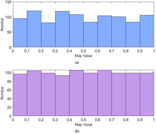
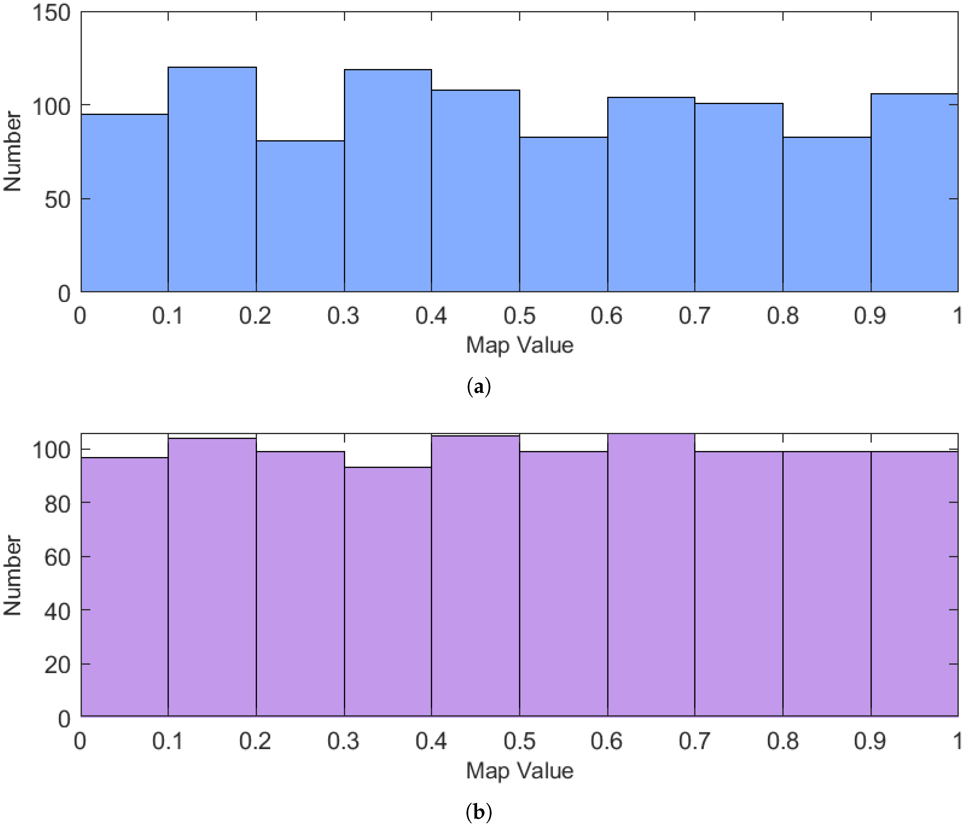
According to Equations (1) and (14), the population distribution histogram generated by random and Tent mapping can be obtained, as shown in Figure 1. Through comparative analysis, the construction of the initial population is carried out under the premise that the population scale is 1000 and the dimension is 1, and the numerical range is 0 to 1. Comparative evaluation shows that compared with random population initialization, the population generated by Tent chaotic map shows better distribution uniformity.

Figure 1. Population initialization comparison (a) Random population initialization. (b) Tent population initialization.

3.2. Location Update Strategy Integrating Multi-Source Directional Information

In the original SH5N1 algorithm, the virus movement direction in the infection diffusion stage only depends on the differential direction of the global optimal solution $F_g$ and the local historical optimal solution $F_p$, and the step vector generated by random disturbance. The corresponding update rule is shown in Equation (6). This strategy is a centralized greedy search strategy in essence, and the pursuit of fast convergence. However, in complex multimodal problems, the single direction information leads to the lack of direction diversity, and the population is easy to gather around a few individuals prematurely, which affects the ability of the algorithm to jump out of local optimum and fine development. In order to enhance the diversity of search directions and the ability of local cooperative convergence, this paper improves the location update strategy. On the basis of retaining the global best and individual historical best information, the local field search mechanism is introduced, the best individual information in the neighborhood is added, and the vector of multi-source direction information is constructed to realize more flexible direction control.

3.2.1. Constructing Neighborhood Optimal Individuals

Let the current population size be n, the current position of the ith virus at iteration t be denoted as $x_i^t$, its historical optimal position be denoted as $F_{p,i}^t$,it, and the neighborhood size be k($k\ll n$). The steps to construct the neighborhood optimal solution for the ith virus are as follows.

Randomly select k (take k = 5 in this article) individuals from $\left\{1,2,\dots ,n\right\}$ to form a neighborhood index set:

$$N_i^t=R\mathrm{an}domsample(\left\{1,2,\dots ,n\right\},k)$$

(15)

where $N_i^t$ represents the set of neighborhood indexes randomly selected by the ith virus in the tth iteration, and $Rdomsample(S,k)$ represents the random selection of k elements from the set S without replacement.

In the neighborhood set $N_i^t$, the individual index with minimum fitness is selected according to the fitness function $f(·)$:

$$j_i^{*}=arg\underset{j\in N_i^t}{min}f\left(F_{p,j}^t\right)$$

(16)

Denote its historical optimal position as the neighborhood optimal position of the ith virus

$$x_{i,loc}^t=F_{p,j_i^{*}}^t$$

(17)

3.2.2. Constructing the Fusion Vector of Multi-Source Directional Information

After obtaining the optimal position in the neighborhood, the global optimal direction, the individual historical optimal direction and the optimal direction in the neighborhood are weighted and fused to construct the multi-source direction information vector $D_j^i$ of the ith virus in the tth iteration:

$$D_j^i=0.6(F_{\mathrm{g},j}-F_{p,j}^i)+0.2(F_{p,j}^i-x_j^i)+0.2(x_{i,loc}^t-F_{p,j}^i)$$

(18)

where the first term refers to the original trend that the current position is close to the global optimal environment, and its weight coefficient is 0.6. The second term reflects the local exploitation behavior of individuals approaching their own historical optimal solution, and its weight coefficient is 0.2. The third term represents the position of the best performing individual in the guided reference neighborhood, reflecting the local cooperative search, and its weight coefficient is also 0.2.

3.2.3. New Position Update Formula for the Infection Transmission Phase

The constructed vector of multi-source direction information is fused into the position update formula of the infection spreading stage:

$$\left\{\begin{array}{cc}{x}_j^i(t+1)=pm{p}_{3,j}^i+{\mathrm{R}}_j^i·D_j^i& p_{attack}<p_1\\ x_j^i\mathrm{t}+1=x_j^i\left(t\right)+{\displaystyle \frac{{\mathrm{R}}_j^i·(pm{p}_{1,j}^i-pm{p}_{2,j}^i)+{\mathrm{R}}_j^i·D_j^i}{2}}& p_{attack}\ge p_1\end{array}\right.$$

(19)

Under the premise of maintaining the biological meaning of the original algorithm, the location update strategy proposed in this paper introduces the information of the neighborhood optimal solution, fuses the information of the global optimal, the individual historical optimal and the neighborhood optimal three directions. When the individual finds the potential excellent region, it can converge to the high-quality solution more quickly under the guidance of the three directions of the global optimal, the historical optimal and the neighborhood optimal. It can improve the local collaborative convergence ability and solution accuracy, reduce the number of iterations required from discovering the excellent region to convergence, and further accelerate the convergence speed of the algorithm.

3.3. Logistic Chaos-Enhanced Variable Step-Size Control Strategy

The original variable step size control factor c employed an exponential decay with $c=r_c·e^{-4\ast {\displaystyle \frac{t}{T}}}$, resulting in rapid attenuation that could prematurely terminate the algorithm’s global exploration phase. To address this, this paper proposes a chaotic-enhanced variable step size control factor optimization strategy. First, the exponential decay coefficient is adjusted from 4 to 2 to slow c’s decay rate and prolong the exploration phase. simultaneously replacing the original random factor $r_c$ with the sequence $g_k$ generated by the Logistic chaotic map. This enhances diversity, inducing non-periodic chaotic fluctuations of c within the interval [0, 1], thereby improving step size diversity and global search capability. The calculation formula for the Logistic chaotic-enhanced variable step size control factor $c_L$ is:

$$c_{\mathrm{L}}={\mathrm{g}}_k·e^{-2·{\displaystyle \frac{t}{T}}}$$

(20)

The logistic mapping $g_k$ is expressed as:

$${\mathrm{g}}_{k+1}=g_k·\mu ·(1-g_k),k=0,1,\dots ,k,\mu \in (0,4],g_k\in \left(0,1\right)$$

(21)

where $g_k$ represents the population state of generation k, and $g_{k+1}$ represents the population state of generation $k+1$. Here, the population state is normalized to the interval (0, 1), where 0 signifies extinction and 1 denotes the maximum population size the environment can sustain. $\mu$ is the growth parameter, set to $\mu =4$ in this paper.

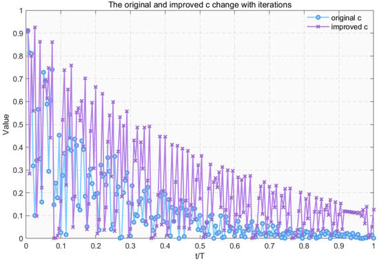
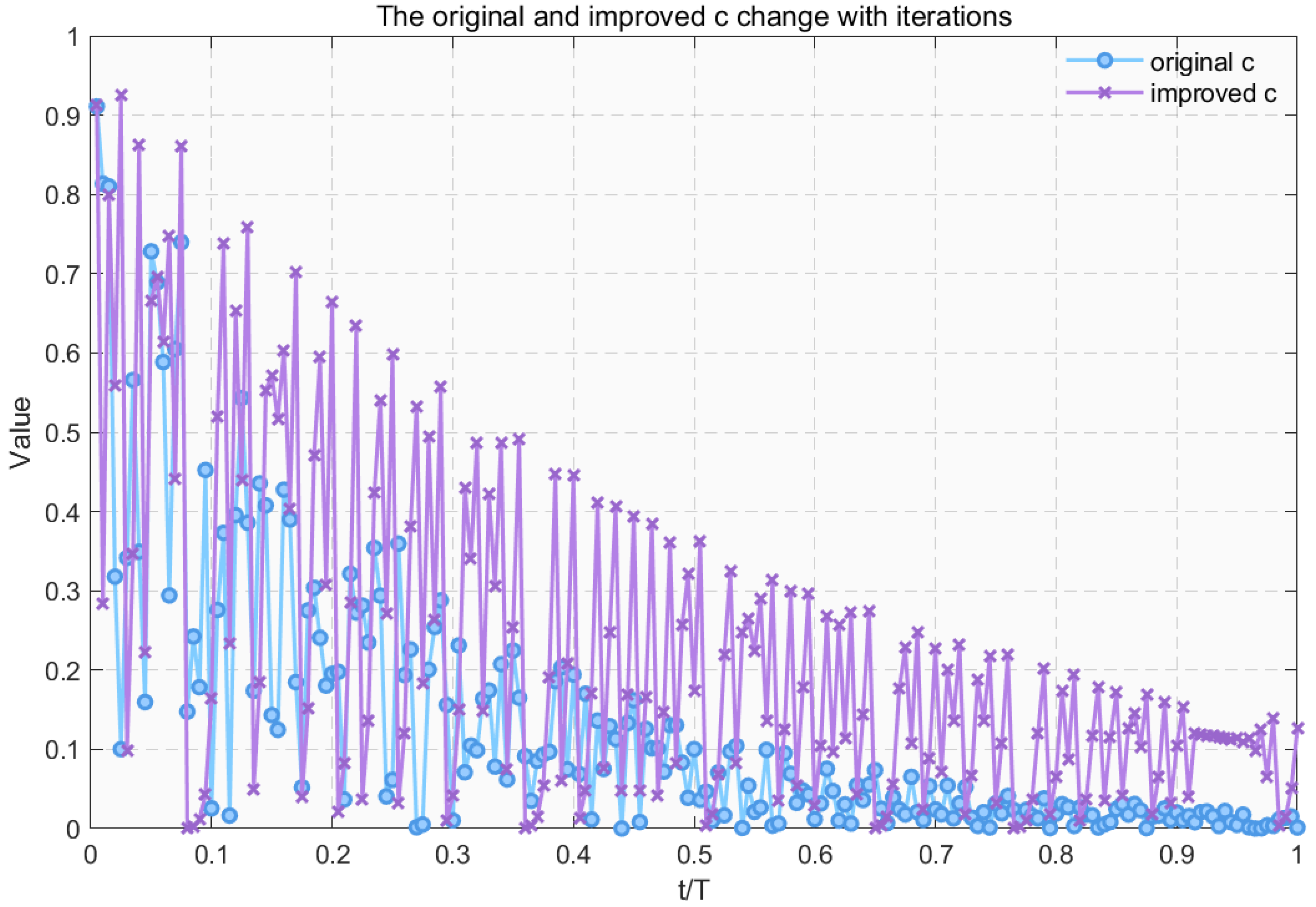
To more intuitively demonstrate the effectiveness of the optimized control factor c for variable stride length, with $T=200$ iterations, we plot the comparison of the original and optimised mutation step size control factor C versus iteration count based on Equations (8) and (20), as shown in Figure 2. The figure reveals that the mutation step size control factor $c=r_c·e^{-4\ast {\displaystyle \frac{t}{T}}}$ in the original SH5N1 algorithm decreases rapidly with a large exponential decay coefficient of 4, showing good performance in the early iterations but rapidly decaying in the middle stage. After reaching 50% of the iteration process, its value oscillates slightly between 0 and 0.1, resulting in a short global search phase. In contrast, the improved control factor $c_{\mathrm{L}}={\mathrm{g}}_k·e^{-2·{\displaystyle \frac{t}{T}}}$ in this paper decreases more gradually under a smaller decay coefficient of 2. Driven by the logistic chaotic sequence $g_k$, it exhibits non-periodic chaotic fluctuations. This maintains both a certain amplitude and high diversity in the variable step size throughout the optimization process. This enhances the algorithm’s ability to escape local optima and perform global exploration while suppressing premature convergence.

Figure 2. Comparison of Iterative Curves for c (Original Method vs. Improved Method).

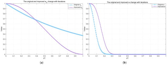
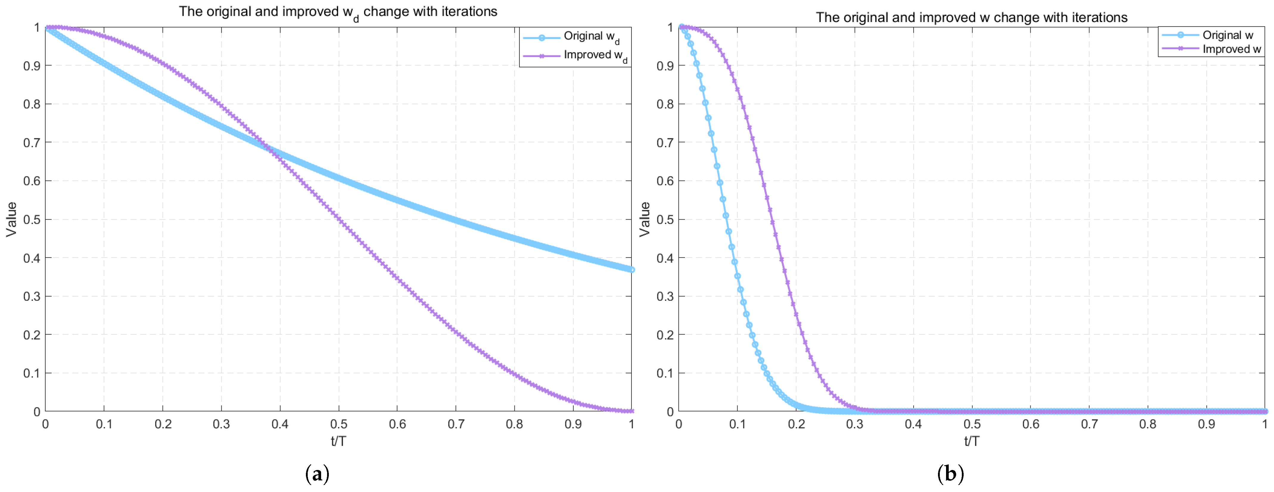
3.4. Optimization of Inertial Weight Decay Coefficient

In the original SH5N1 algorithm, the inertia weight decay coefficient wd employs a fixed exponential decay form $w_d\left(t\right)=w_{min}+(w_{max}-w_{min})·e^{-\left({\displaystyle \frac{t}{T}}\right)}$, featuring a uniform decay rate. This makes it challenging to balance early-stage global exploration and late-stage local exploitation during complex searches. To enhance search phase equilibrium, this paper introduces a cosine annealing strategy to modify the inertia weight decay coefficient $w_d$, as shown in Equation (22). Cosine annealing is a strategy that gradually reduces weight coefficients using a cosine function. The cosine function exhibits a characteristic where its value increases initially at a relatively gentle slope, accelerates rapidly as iterations progress, and then levels off again. Leveraging this behavior, the cosine annealing strategy is incorporated into the inertial weight decay coefficient $w_d$, yielding the improved form:

$$w_d\left(t\right)=w_{min}+{\displaystyle \frac{1}{2}}(w_{max}-w_{min})[1+cos({\displaystyle \frac{\mathrm{t}}{T}}\pi )]$$

(22)

where $w_d$ denotes the weight decay coefficient; $w_{m}in$ and $w_{m}ax$ represent its minimum and maximum values; T denotes the maximum iteration count, and t represents the current iteration count. This formulation ensures that while $w_d\in [w_{min},w_{max}]$, the inertia weight exhibits more controllable and smoother variation from the early to mid-stage, facilitating a balance between global search and local exploration. In the mid-to-late stages, the inertia weight decays more rapidly, enabling finer local search and achieving faster, more stable convergence.

To more intuitively demonstrate the effectiveness of the aforementioned inertia weight decay parameter improvement strategy, this paper selects the maximum iteration count and calculates $w_d$ using both the original exponential decay form and the cosine annealing form given by Equation (22). Based on this, the corresponding inertial weight w is obtained by recursion. Figure 3a presents the curves of the two values $w_d$ as a function of the iteration count, while Figure 3b illustrates the decay process of the corresponding inertial weight w.

Figure 3. Comparison of original and improved inertial weight decay strategies. (a) Inertial weight decay coefficient iteration curve. (b) Inertial weighting iteration curve.

As shown in Figure 3a, the exponential decay coefficient $w_d$ in the original SH5N1 exhibits an approximately monotonically linear decrease, declining relatively uniformly throughout the search process while maintaining a relatively high level of approximately 0.37 in the later stages. In contrast, the improved cosine annealing coefficient $w_d$ decays slowly in the early stages, decreases rapidly in the middle stages, and rapidly approaches $w_{min}$ near the end of iterations. This indicates that cosine annealing maintains a larger weight coefficient in the early stages to enhance global search capability, while promptly reducing the weight in the middle and late stages to facilitate local convergence. The Figure 3b compares the variation of the recursively obtained inertial weight w under the two strategies. It is evident that the original weight decays to near zero around 0.2 T, resulting in a short duration of effective inertial effects and a tendency for the search to prematurely transition into a conservative local exploitation phase. In contrast, the improved weight maintains a non-zero value over a longer mid-stage iteration period before rapidly decaying to near zero. This approach extends the global exploration phase while ensuring stable convergence in the later stages. In summary, the cosine annealing-based inertia weight decay strategy demonstrates significant advantages over the original exponential decay form in balancing global search and local exploitation, as well as suppressing premature convergence.

3.5. Time Complexity Analysis

Given a population size N, dimension D, and maximum iteration count T, the time complexity of a single fitness function calculation is denoted as F, and the neighborhood size as k. The original SH5N1 algorithm’s time complexity can be summarized as follows: generating D-dimensional positions for N individuals requires $O\left(ND\right)$, while calculating each individual’s fitness requires $O\left(NF\right)$. Thus, the initialization phase complexity is $O(ND+NF)\approx O\left(NF\right)$. In each iteration, updating positions, applying mutations, and boundary handling for each individual primarily involve constant-order and $O\left(D\right)$ linear operations; Recalculating fitness for all individuals incurs $O\left(NF\right)$ complexity. Thus, the per-generation complexity is $O(NF+ND)\approx O\left(NF\right)$. Consequently, the overall time complexity of the original SH5N1 algorithm is $O(NF+T(NF+ND\left)\right)\approx O\left(TNF\right)$.

The improved SH5N1 algorithm incorporates Tent chaotic initialization during the initialization and position update phases. The Tent map essentially performs a constant-time iteration for each dimension, maintaining a complexity of $O\left(ND\right)$. Subsequent calculations still require computing the fitness of all individuals, $O\left(NF\right)$. Therefore, the complexity of the initialization phase is $O(ND+NF)\approx O\left(NF\right)$, which is identical in magnitude to the original SH5N1. Within the main loop, the vector computation process for multi-source directional information proceeds as follows: For each individual, a neighborhood set (size k) is randomly selected with a complexity of $O\left(k\right)$. Finding the most fit individual within the neighborhood requires $O\left(k\right)$. Subsequently, a direction vector is computed comprising the global optimum, the individual’s historical optimum, and the neighborhood optimum. With each dimension being a linear combination, requiring $O\left(D\right)$ complexity. Summing over all individuals, this part has a complexity of approximately $O\left(N\right(k+D\left)\right)$. Since k is a constant, this term can be regarded as an additional overhead of $O\left(ND\right)$ order. Updating the weight decay coefficient $w_d$ and mutation step size control parameter $c_L$ involves only a few scalar operations, resulting in negligible constant-order complexity. Performing position updates, mutations, and boundary handling for all individuals remains a linear operation per dimension, yielding a total complexity of $O\left(ND\right)$. Recalculating fitness for all individuals retains a complexity of $O\left(NF\right)$, remaining the most time-consuming spart of a single iteration. Since the cost of a single fitness evaluation is typically far greater than other linear operations (i.e., $F\gg D+k$), the single-generation complexity of the improved algorithm can be approximated as $O(NF+N(D+k\left)\right)\approx O\left(NF\right)$. Consequently, its overall time complexity is $O(NF+T(NF+N(D+k)\left)\right)\approx O\left(TNF\right)$, which remains on the same order of magnitude as the original SH5N1.

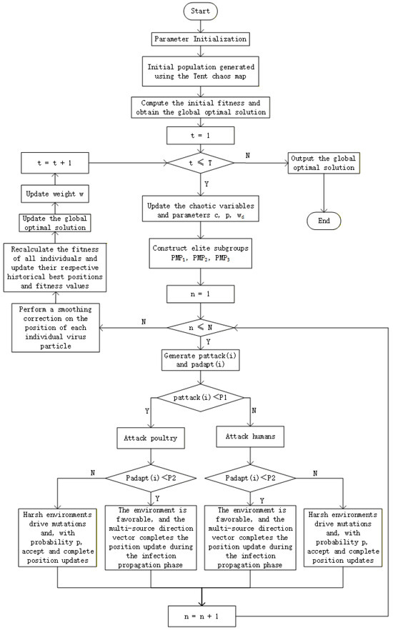
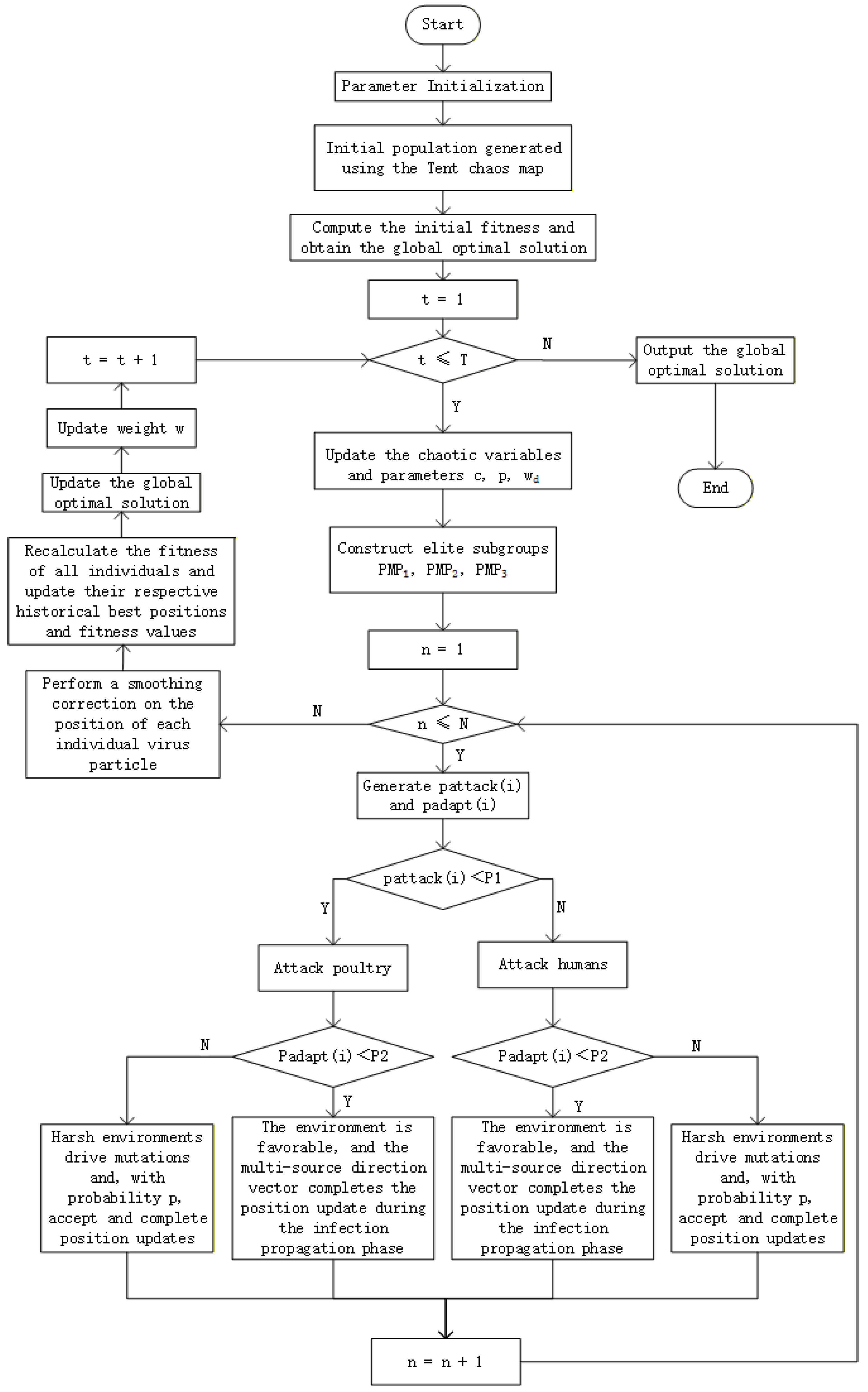
4. Algorithm Implementation Steps and Flowchart

The specific steps of the improved SH5N1 algorithm (hereinafter referred to as ISH5N1) are as follows:

• Step 1: Initialize the fundamental parameters of the ISH5N1 population, including population size N, maximum iteration count T, dimension D, search upper and lower bounds $L_b$ and $U_b$, set the probability $P_1$ of viral attack on birds, the survival probability $P_2$ of the virus after host infection, inertia weight upper and lower bounds $w_{min}$ and $w_{max}$, domain size k, as well as control parameters such as the Logistic mapping and mutation acceptance probability.
• Step 2: Using Tent chaos initialization involves generating chaotic sequences for each dimension via the Tent mapping, then linearly mapping the results to $[L_b,U_b]$ to obtain the optimal positions for the initial individuals.
• Step 3: Evaluate the fitness value of each individual in the initial population, record the historical best fitness and position for each individual, and determine the global optimum solution.
• Step 4: Each generation updates control parameters during iteration by applying the Logistic mapping to update chaotic variables, calculating the adaptive mutation step size factor $c_L$, mutation acceptance probability p, and the cosine annealing-based inertia weight decay coefficient $w_d$. The inertia weight is then updated via $w(t+1)=w\left(t\right)·w_d\left(t\right)$. For each individual, randomly generate the attack probability $P_{attack}$ and the adaptation probability $P_{adapt}$.
• Step 5: Based on the historical optimal positions of all individuals, the index vectors undergo cyclic shifts according to Equations (2)–(5), constructing three permutation elite matrices $PM{P}_1$, $PM{P}_2$, and $PM{P}_3$. These matrices provide diverse reference directions for subsequent position updates.
• Step 6: By comparing each viral particle’s $P_{attack}$, $P_{adapt}$, $P_1$, $P_2$, and size to select targets and evaluate the environment, viral growth is facilitated, with particles updating solely according to Equation (19); Harsh environments drive viral mutations for adaptation, implemented via Equation (7). Solution acceptance is determined by mutation selection probability p and random acceptance threshold ps, achieved through Equation (11). Subsequently, each viral particle’s position undergoes smoothing correction as shown in Equation (10).
• Step 7: Recalculate the fitness of all individuals, update their respective historical optimal positions and fitness values, and update the global optimal solution whenever a better individual is discovered.
• Step 8: When the iteration count reaches the upper limit T, the algorithm terminates; otherwise, return to step 4 to continue searching for the next generation. Upon algorithm completion, output the final global optimal position and its fitness value.

The flowchart of the ISH5N1 algorithm is shown in Figure 4:

Figure 4. Flowchart of the ISH5N1 Algorithm.

5. Simulation Experiments and Analysis

The simulation experiments for the ISH5N1 algorithm primarily consist of two parts: comparative analysis under standard benchmark functions and global path planning simulations. To evaluate the performance of the proposed ISH5N1 algorithm, all simulations were conducted on the same hardware and software platform. The hardware platform comprised a laptop equipped with an Intel® Core™ i7-8750 processor (base frequency 2.21 GHz) and 16 GB RAM. The software environment included the Windows 11 operating system, with algorithm simulations and testing performed in the MATLAB 2023b environment.

5.1. Solving the Classical Functions

To validate the optimization performance of the proposed ISH5N1 algorithm, nine classic test functions with distinct characteristics were selected from internationally recognized test function libraries. A comparative analysis was conducted between the ISH5N1 algorithm proposed in this paper and several common swarm intelligence optimization algorithms. The comparison algorithms are listed in Table 1.

Table 1. Comparison Algorithm.

Abbreviation	Algorithm
DBO	Dung Beetle Optimization Algorithm [31]
WOA	Whale Optimization Algorithm [32]
BOA	Butterfly Optimization Algorithm [33]
SH5N1	H5N1 virus Optimization Algorithm
ISH5N1	Improved SH5N1

Table 2 presents information on nine test functions. Among them, F1–F3 are unimodal functions, designed to evaluate the algorithm’s local exploration capability and convergence accuracy; F4–F6 are multimodal test functions containing numerous local optima, testing the algorithm’s global optimization capability and its ability to overcome local optima; F7–F9 are composite functions with complex structures and strong variable coupling, suitable for evaluating the algorithm’s overall performance and stability. These nine functions, ranging from simple to complex, constitute classic test functions for evaluating optimization algorithm performance.

Table 2. Classical benchmark functions.

Type	Function	Dim	Global Optima
Unimodal function	$F_{1\left(X\right)}={\sum }_{i=1}^n{x}_i^2$	30	0
	$F_{2\left(X\right)}={max}_i\left\{\left|x_i\right|,1\le i\le n\right\}$	30	0
	$F_{3\left(X\right)}={\sum }_{i=1}^{n}i{x}_i^4+random[0,1)$	30	0
Multimodal function	$F_{4\left(X\right)}={\sum }_{i=1}^n\left[x_i^2-10cos\left(2\pi x_i\right)+10\right]$	30	0
	$F_{5\left(X\right)}=-20exp(-0.2\sqrt{{\displaystyle \frac{1}{n}}{\sum }_{i=1}^n{x}_i^2})-exp({\displaystyle \frac{1}{n}}{\sum }_{i=1}^{n}cos(2\pi x_i))+20+e$	30	0
	$F_{6\left(X\right)}={\displaystyle \frac{1}{4000}}{\sum }_{i=1}^n{x}_i^2-{\prod }_{i=1}^{n}cos({\displaystyle \frac{x_i}{\sqrt{i}}})+1$	30	0
Composition function	$F_{7\left(X\right)}={\displaystyle \sum _{i=1}^{11}}{\left[a_i-{\displaystyle \frac{x_1\left(b_i^2+b_1{x}_2\right)}{b_i^2+b_1{x}_3+x_4}}\right]}^2$	4	0.0003075
	$F_{8\left(X\right)}=-{\displaystyle \sum _{i=1}^7}{\left[\left(X-a_i\right){\left(X-a_i\right)}^T+c_i\right]}^{-1}$	4	−10.4029
	$F_{9\left(X\right)}=-{\displaystyle \sum _{i=1}^{10}}{\left[\left(X-a_i\right){\left(X-a_i\right)}^T+c_i\right]}^{-1}$	4	−10.5364

To ensure the validity, reliability, and accuracy of the experimental results, the population size and maximum iteration count for all algorithms were set to identical values. This study set the population size to 50 and the maximum iteration count to 500, with other internal parameters consistent with the original literature. The five methods described above were applied to solve all functions listed in Table 2. To mitigate the impact of randomness on test results, each algorithm was independently run 30 times for every function.

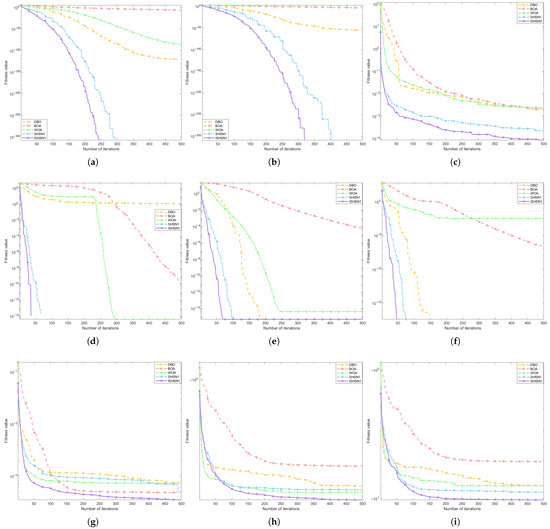
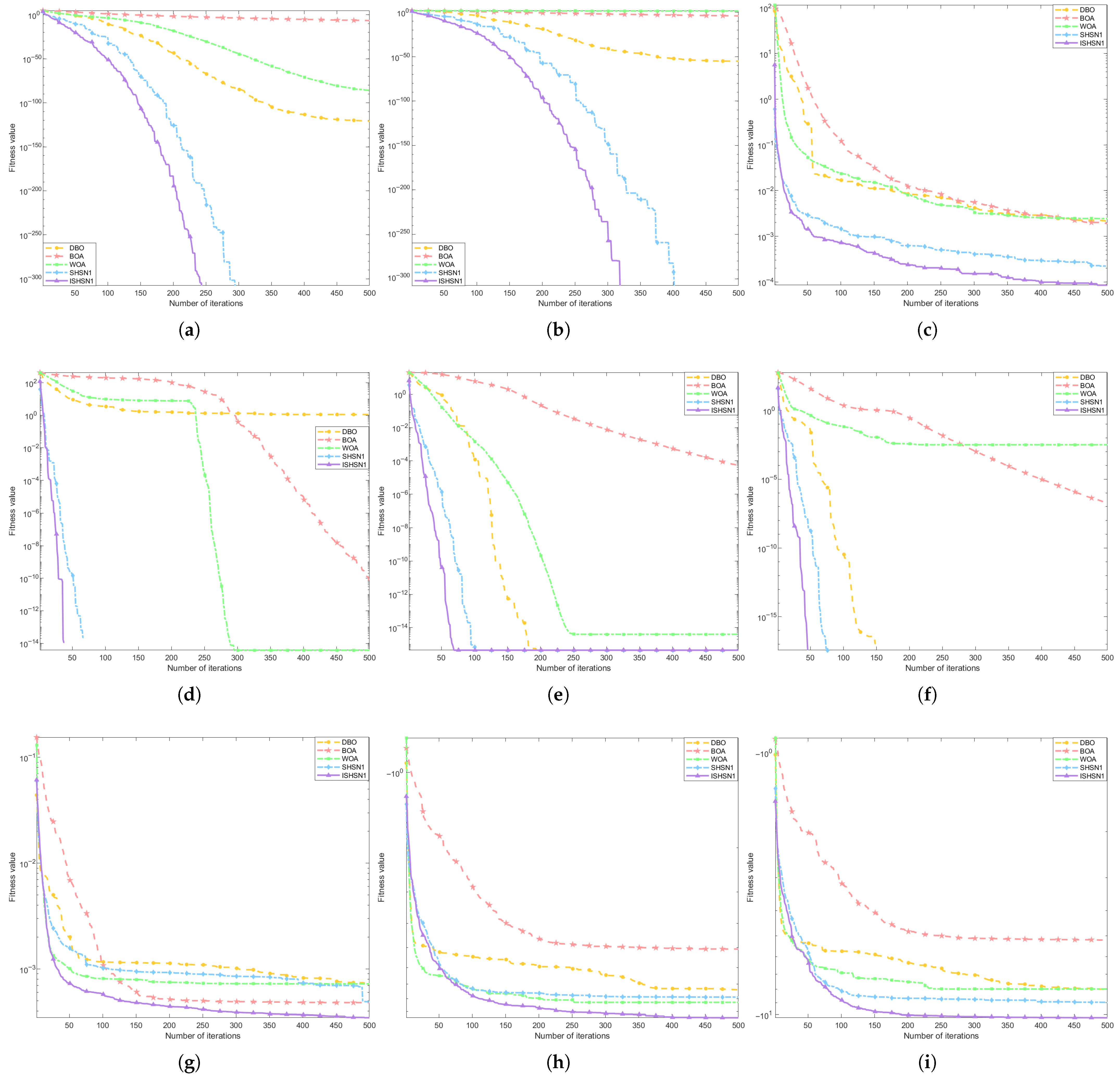
Figure 5 displays the average fitness variation curves of five algorithms across nine test functions. Table 3 lists the optimal values, mean values, and standard deviations achieved by each algorithm across all test functions. The trend of the fitness curve serves as an evaluation metric for algorithm convergence speed, while the optimal value, mean value, and standard deviation respectively serve as evaluation metrics for the algorithm’s search capability, search stability, and dispersion. A smaller mean indicates stronger convergence accuracy and optimization capability; a smaller standard deviation signifies less algorithmic fluctuation and more stable performance.

Figure 5. Classical functions convergence curves. (a) F1 convergence curve. (b) F2 convergence curve. (c) F3 convergence curve. (d) F4 convergence curve. (e) F5 convergence curve. (f) F6 convergence curve. (g) F7 convergence curve. (h) F8 convergence curve. (i) F9 convergence curve.

Table 3. Comparison of optimization results of different intelligent algorithms.

Function	Index	DBO	BOA	WOA	SH5N1	ISH5N1
$F_1$	Best	1.2546 × 10−181	1.4291 × 10−07	6.7922 × 10−94	0	0
	Mean	1.2375 × 10−121	2.8022 × 10−07	1.3408 × 10−86	0	0
	Std	6.3784 × 10−121	7.5095 × 10−08	2.9068 × 10−85	0	0
$F_2$	Best	1.7350 × 10−84	5.4525 × 10−05	5.2430 × 10−04	0	0
	Mean	8.6690 × 10−56	7.7254 × 10−05	32.8673	0	0
	Std	4.4059 × 10−55	1.4906 × 10−05	31.1144	0	0
$F_3$	Best	4.7511 × 10−05	8.5037 × 10−04	7.0203 × 10−05	1.0782 × 10−05	1.9742 × 10−06
	Mean	2.1579 × 10−03	1.9231 × 10−03	2.4445 × 10−03	2.2297 × 10−04	8.5076 × 10−05
	Std	1.7960 × 10−03	5.8717 × 10−04	3.3235 × 10−03	1.6568 × 10−04	6.4059 × 10−05
$F_4$	Best	0	0	0	0	0
	Mean	1.1276	7.3237 × 10−11	3.7896 × 10−15	0	0
	Std	4.6648	1.7768 × 10−10	2.0756 × 10−14	0	0
$F_5$	Best	4.4409 × 10−16	3.3588 × 10−05	4.4409 × 10−16	4.4409 × 10−16	4.4409 × 10−16
	Mean	4.4409 × 10−16	5.3992 × 10−05	3.9968 × 10−15	4.4409 × 10−16	4.4409 × 10−16
	Std	0	1.0589 × 10−05	2.2853 × 10−15	0	0
$F_6$	Best	0	3.8583 × 10−08	0	0	0
	Mean	0	1.5423 × 10−07	2.3520 × 10−03	0	0
	Std	0	9.4182 × 10−08	1.2882 × 10−02	0	0
$F_7$	Best	3.0777 × 10−04	3.6223 × 10−04	3.1087 × 10−04	3.1054 × 10−04	3.0749 × 10−04
	Mean	7.3144 × 10−04	4.8181 × 10−04	7.2396 × 10−04	4.9160 × 10−04	3.4830 × 10−04
	Std	3.3643 × 10−04	7.9791 × 10−05	4.3072 × 10−04	4.1828 × 10−04	5.6270 × 10−05
$F_8$	Best	−10.4029	−7.3572	−10.4028	−10.4029	−10.4029
	Mean	−7.3614	−5.0638	−8.2637	−7.8772	−9.5042
	Std	2.7169	5.2369 × 10−01	2.9303	2.6074	1.8738
$F_9$	Best	−10.5364	−8.1437	−10.5360	−10.5364	−10.5364
	Mean	−8.0119	−5.1886	−7.9856	−8.9914	−10.2647
	Std	2.7452	7.6526 × 10−01	3.2426	2.3486	1.0124

Based on the analysis of the average iteration curves for different algorithms after 30 runs shown in Figure 5, ISH5N1 performs well on most test functions. As demonstrated in Figure 5a,b,d–f, ISH5N1 converges significantly faster than other comparison algorithms. Compared to the original SH5N1, ISH5N1 exhibits steeper initial descent and a more pronounced curve, indicating that Tent chaotic initialization enhances the quality of the initial solution distribution. The position update strategy, which integrates multi-source directional information, accelerates effective convergence in the search direction. Compared to DBO, BOA, and WOA, ISH5N1 enters the stable descent phase earlier, demonstrating superior search efficiency. In composite functions (e.g.Figure 5g–i), most comparison algorithms exhibit convergence stagnation or oscillations in the mid-to-late stages. Conversely, the ISH5N1 curve remains lower than other algorithms while maintaining a sustained downward trend, gradually approaching the optimal solution with minimal late-stage fluctuations. This indicates that the incorporated multi-source directional information effectively suppresses blind search behavior. The logistic chaos-enhanced variable step size control strategy enhances the algorithm’s ability to escape local optima. The inertia weight decay coefficient, fused with the cosine annealing strategy, prolongs the global exploration phase while ensuring stable convergence in the later stages. Under the same number of iterations, the ISH5N1 algorithm achieves superior optimization results.

The performance of the five algorithms was quantitatively compared based on three metrics: optimal value, average value, and standard deviation. For the test functions F1, F2, F4, and F6, Both ISH5N1 and SH5N1 consistently achieve theoretical optimal solutions. DBO, BOA, and WOA exhibit varying degrees of deviation in optimal values and average values. For certain functions (e.g., F3, F7), ISH5N1 obtains optimal values significantly superior to other comparison algorithms and outperforms the original SH5N1, indicating that the improved strategy further enhances solution accuracy in complex search spaces. The standard deviation metric reveals that ISH5N1 exhibits the smallest or near-smallest standard deviation across most test functions, indicating highly consistent results across multiple independent runs. In contrast, DBO and BOA show larger standard deviations on multi-peaked and composite functions, resulting in unstable outcomes. WOA tends to get stuck in local optima on some functions, leading to noticeable solution fluctuations. On composite functions such as F7, F8, and F9, ISH5N1 outperforms the comparison algorithms in both optimal values and average performance, demonstrating particularly significant advantages in average performance. This indicates the algorithm possesses stronger adaptability and generalization capabilities for complex problems.

In summary, the ISH5N1 algorithm demonstrates significant advantages in convergence speed, solution accuracy, and stability. By incorporating Tent chaotic initialization, a position update strategy integrating multi-source directional information, and an improved inertial weighting and variable stride control mechanism, the algorithm maintains strong global exploration capabilities during the early search phase while rapidly converging toward the optimal region in the mid-to-late stages, effectively avoiding premature convergence. Compared to DBO, BOA, WOA, and the original SH5N1, ISH5N1 achieves superior optimal values and average results on most test functions while exhibiting smaller standard deviations. This demonstrates that the proposed improvements enhance the algorithm’s overall performance, validating its effectiveness and robustness in tackling complex high-dimensional optimization problems.

5.2. Path Planning Simulation Experiment

This section applies the ISH5N1 algorithm to simulate robots solving shortest path problems in grid maps. To evaluate the feasibility and effectiveness of ISH5N1 in path planning, experimental results are compared with five traditional algorithms: the H5N1 virus optimization algorithm (SH5N1), Dung Beetle Optimization Algorithm (DBO), Whale Optimization Algorithm (WOA), and Butterfly Optimization Algorithm (BOA). To ensure fairness and validity, the population size and iteration count for all algorithms were uniformly set to 50 and 200, respectively. Additionally, all other internal parameters for each algorithm were configured identically to their original literature specifications.

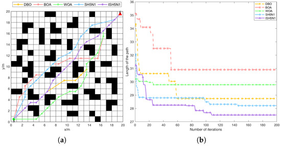
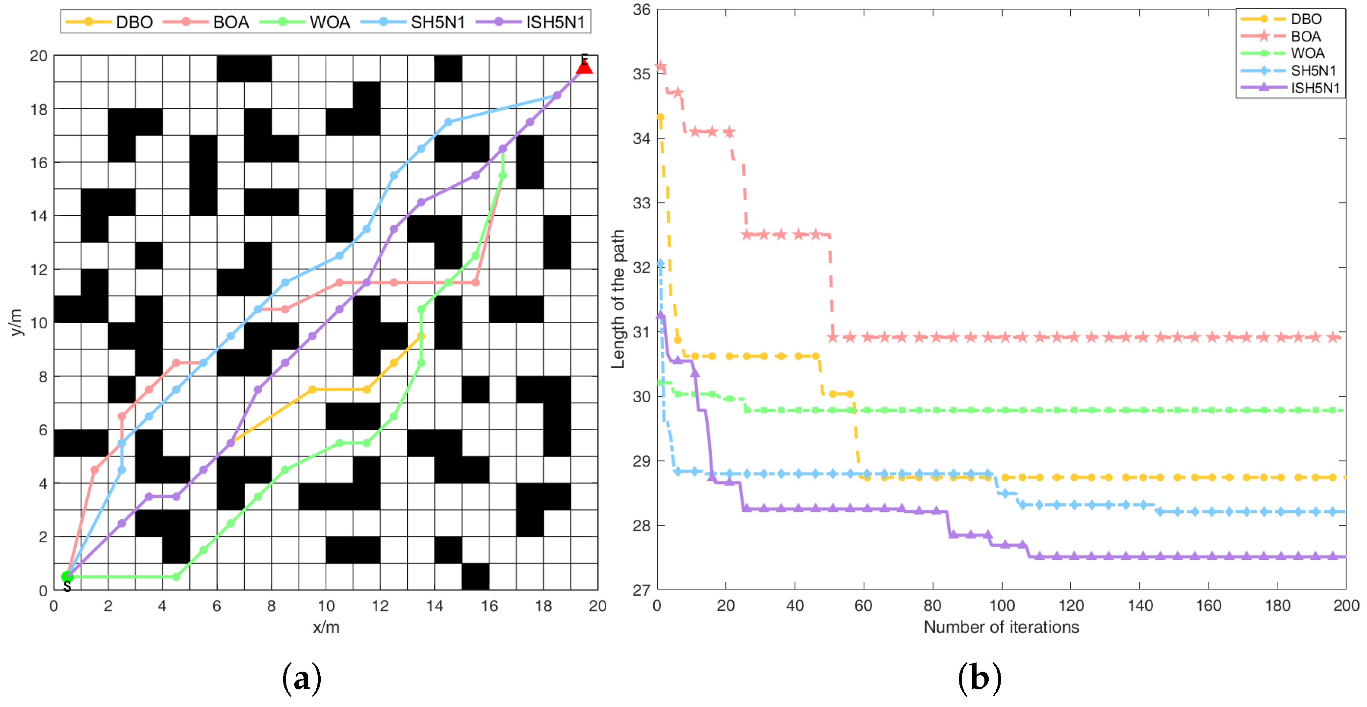
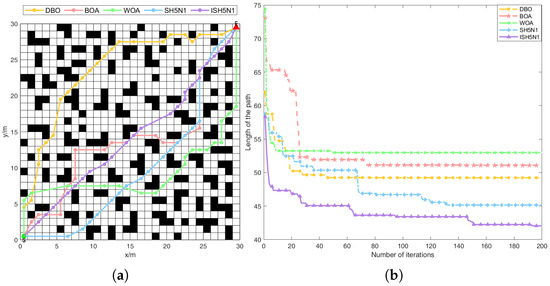
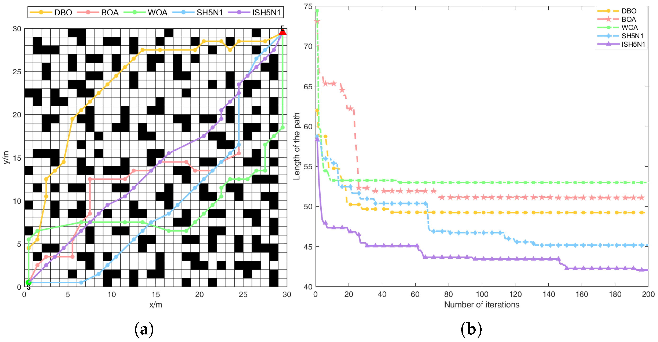
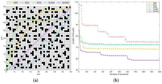
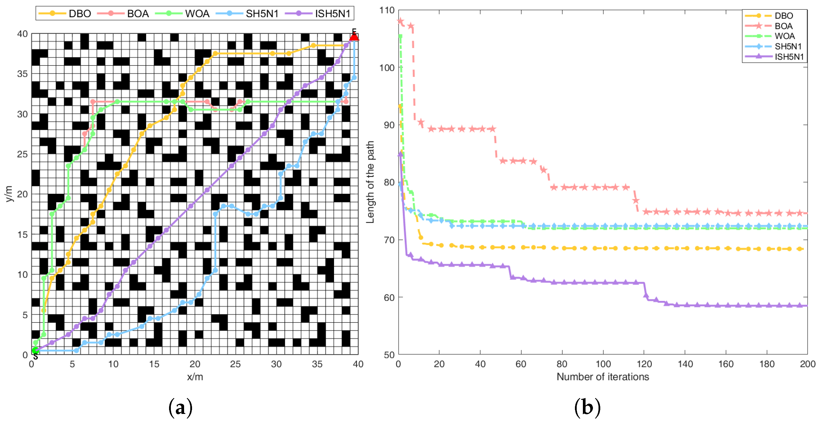
Figure 6, Figure 7 and Figure 8 show comparative simulation experiments of the five algorithms on three different grid map sizes: Environment 1 (20 × 20), Environment 2 (30 × 30), and Environment 3 (40 × 40). The small green circle S denotes the starting point, the red triangle E indicates the destination, black areas represent obstacles, and white boxes mark navigable regions. The three map sizes progressively increase in environmental complexity, placing escalating demands on the algorithms’ path planning capabilities. This setup effectively evaluates algorithm performance across varying environments.

Figure 6. Comparison Results in Environment 1. (a) Results of running in Environment 1. (b) Convergence curve in Environment 1.

Figure 7. Comparison Results in Environment 2. (a) Results of running in Environment 2. (b) Convergence curve in Environment 2.

Figure 8. Comparison Results in Environment 3. (a) Results of running in Environment 3. (b) Convergence curve in Environment 3.

Figure 6a, Figure 7a and Figure 8a show the path planning simulation results for each algorithm in different environments, while Figure 6b, Figure 7b and Figure 8b display the path planning convergence curves for each algorithm in the respective environments. From the path planning simulation results, all algorithms successfully planned feasible paths from start to finish across three grid environments of varying complexity. However, trajectories generated by DBO, BOA, WOA, and SH5N1 generally exhibited some degree of backtracking and detours, resulting in relatively winding and circuitous paths. Compared to other algorithms, the ISH5N1 algorithm produced paths with fewer turns, overall smoother trajectories, and shorter lengths. Moreover, as environmental complexity increased, it still managed to plan relatively straight paths with minimal redundant segments even in densely obstructed areas. In contrast, algorithms like BOA and DBO exhibit significantly more detours and turning points in their found paths. As shown in Figure 8a, the path found by SH5N1 even displays a noticeable “backtracking” phenomenon, further increasing the path length.

Analysis of the convergence curve reveals that the ISH5N1 algorithm achieves a low path length within a small number of iterations. It continues to make minor refinements during subsequent iterations, exhibiting a “secondary descent” in the middle phase of iteration. This sustained movement toward a better solution demonstrates its strong ability to escape early local optima and persistently explore more optimal solutions. In contrast, other algorithms become trapped in higher local optima early on, showing no significant further decline after reaching a certain level. resulting in relatively large final convergence values and exhibiting premature convergence issues.

It can be observed that under all three scenarios, ISH5N1 achieves the shortest final path with smoother trajectories and fewer turning points. Compared to DBO, BOA, WOA, and SH5N1, it exhibits significantly reduced detours and redundant segments, demonstrating superior path optimization capabilities. ISH5N1 exhibits a faster descent rate during the early iteration phase and further refines the path through meticulous search in the later stages. The final convergence value is stable with minimal curve fluctuations, indicating that the algorithm achieves a better balance between exploration and exploitation. As the environment escalated from simple to complex, other algorithms exhibited noticeable degradation in path length and convergence performance. In contrast, ISH5N1 maintained relatively stable performance across all three environments, consistently outperforming the comparison algorithms. This demonstrates the algorithm’s superior robustness and scalability in adapting to variations in environmental scale and obstacle distribution.

In summary, the ISH5N1 algorithm proposed in this paper demonstrates superior global search capabilities, enhanced ability to escape local optima, and improved convergence accuracy and stability compared to DBO, BOA, WOA, and SH5N1 when addressing path planning problems in raster map environments. It can generate high-quality paths under various complex environmental conditions.

To account for the impact of randomness on experimental outcomes, multiple simulation experiments were conducted. Each algorithm was independently run 20 times across three map environments to determine the minimum, average, and standard deviation values for path length, as well as the minimum, average, and standard deviation values for iteration count. A comprehensive evaluation of the algorithms’ optimization results in path planning problems was performed. The experimental results are presented in Table 4.

Table 4. Comparison of algorithms in different environments.

Environment	Algorithm	Path Length			Number of Iterations
		Best	Mean	Std	Best	Mean	Std
Environment 1 (20 × 20)	DBO	27.8410	28.9699	0.55116	7	50.40	58.08
	BOA	29.2198	29.8337	0.46788	27	117.40	58.43
	WOA	28.5312	29.3784	0.58196	5	47.70	41.30
	SH5N1	27.5072	28.6218	0.82654	41.30	97.85	56.33
	ISH5N1	27.5072	27.8829	0.54785	37	96.55	55.64
Environment 2 (30 × 30)	DBO	42.0122	47.0767	3.0317	11	89.10	74.33
	BOA	46.5849	50.9853	1.6259	35	122.55	48.44
	WOA	44.9859	49.9404	2.1822	10	80.85	50.25
	SH5N1	43.1548	46.1594	2.2155	32	115.65	49.73
	ISH5N1	41.6493	42.7491	1.2148	20	120.80	54.87
Environment 3 (40 × 40)	DBO	62.8226	71.2649	3.0485	4	94.45	72.62
	BOA	73.0226	74.3869	1.0620	76	167.75	38.22
	WOA	68.0873	70.9529	1.0341	14	63.60	48.19
	SH5N1	66.8990	70.3742	1.2840	36	113.95	58.87
	ISH5N1	55.9828	57.7505	1.2872	45	150.80	43.02

In terms of path length, ISH5N1 consistently exhibited the shortest average path length across all three environments. In environments 1–3, its average path lengths were 27.8829, 42.7491, and 57.7505, respectively. Compared to DBO, these values represent reductions of 3.75%, 9.19%, and 18.96%, respectively. Compared to BOA, the reductions were 6.54%, 16.15%, and 22.36%, respectively. Compared to WOA, the reductions were 5.09%, 14.40%, and 18.61%, respectively. and improved by approximately 2.58%, 7.39%, and 17.94% compared to the original SH5N1. The results demonstrate that as the environment scale expands from 20 × 20 to 40 × 40, the ISH5N1 algorithm consistently finds shorter paths when handling path planning problems of varying scales. Compared to other algorithms, its advantages gradually increase with rising environmental complexity, showcasing its strong path optimization capabilities and stability in addressing path planning challenges.

To evaluate how algorithms maintain their advantages as raster size increases, this paper introduces the relative degradation rate, which represents the percentage loss in relative advantage of the ISH5N1 algorithm compared to other methods for every 10 × 10 increase in raster size. When scaling from 20 × 20 to 30 × 30, ISH5N1 exhibits relative degradation rates of −145.00%, −147.05%, −182.88%, and −186.18% relative to DBO, BOA, WOA, and SH5N1 at 20 × 20 → 30 × 30 were −145.00%, −147.05%, −182.88%, and −186.18%, respectively. At 30 × 30 → 40 × 40, the relative degradation rates were −106.29%, −38.45%, −29.22%, and −142.80%. The results indicate that during the expansion process where both segments (20 × 20 → 30 × 30 and 30 × 30 → 40 × 40) exhibit negative relative degradation rates, the relative advantage of ISH5N1 did not degrade but instead showed an overall expansion trend, demonstrating excellent robustness.

In terms of the shortest path metric, the ISH5N1 algorithm achieved superior solutions across all three environments. In Environment 1, it matched SH5N1 at 27.5072, while in Environments 2 and 3, it recorded 41.6493 and 55.9828 respectively—the lowest values among all algorithms. The shortest path typically reflects the theoretical upper limit achievable under ideal convergence conditions. The results indicate that the ISH5N1 algorithm is more effective at escaping local optima and finding the true global optimum during the global search phase. Compared to the other four algorithms, under equivalent conditions, the ISH5N1 algorithm has a higher probability of obtaining superior solutions, demonstrating its superior reliability for engineering applications.

The standard deviation of path length reflects the algorithm’s stability. In Environment 2, ISH5N1 achieved a path length standard deviation of 1.2148, the lowest value in this environment, significantly lower than DBO, WOA, and SH5N1. In Environments 1 and 3, the standard deviation of ISH5N1, though not the smallest, remained at a low level, only slightly higher than a few comparison algorithms. This indicates that the ISH5N1 algorithm exhibits minimal fluctuation between multiple runs when handling environments of varying complexity, consistently yielding relatively stable results.

Regarding the number of iterations, although WOA and DBO exhibit relatively fewer average iterations across the three environments, their corresponding path lengths are significantly longer. This indicates that they often become trapped in local optima at an early stage, leading to premature convergence. In contrast, ISH5N1 achieves markedly superior paths with only a moderate increase in iterations. Its average iteration count remains comparable to BOA and SH5N1, while its standard deviation exhibits minimal fluctuation. These results demonstrate that ISH5N1 strikes a better balance between exploration and exploitation: it avoids premature stagnation due to local optima without incurring excessive computational costs.

In summary, Table 4 quantitatively validates the simulation results presented in Figure 6, Figure 7 and Figure 8. Across grid environments of varying scales and complexities, ISH5N1 consistently achieves shorter and more reliable paths within an acceptable number of iterations. Its global optimization capability, convergence accuracy, and adaptability to complex environmental changes outperform DBO, BOA, WOA, and the original SH5N1 algorithm. The ISH5N1 algorithm, enhanced through the introduction of multi-strategy approaches, demonstrates strong adaptability, efficiency, and stability. This validates its practical application value and potential in path planning problems, making it suitable for real-world path planning scenarios demanding high path quality and stability.

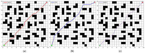
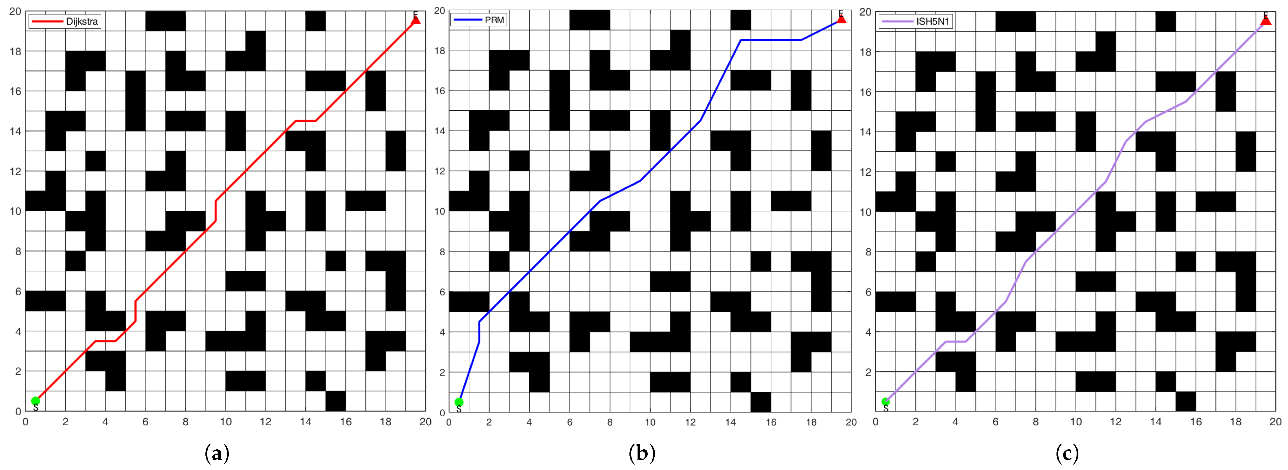
To further validate the applicability and computational efficiency of the proposed ISH5N1 algorithm in classical obstacle avoidance path planning, two representative traditional planners are introduced as benchmarks: the Probabilistic Roadmap Method (PRM) and grid-based Dijkstra search (Dijkstra). It should be noted that PRM and Dijkstra lack internal concepts such as population size and iteration count used in intelligent optimization algorithms. Therefore, this paper employs universal planning metrics applicable to both types of algorithms for comparison, including path length and runtime. To ensure fairness, all algorithms were run in Environment 1 (20 × 20). For stochastic algorithms (ISH5N1 and PRM) and deterministic algorithms (Dijkstra), each was independently run 20 times under identical settings, with results averaged. Figure 9a–c shows path planning simulation results for the Dijkstra, PRM, and ISH5N1 algorithms, respectively. Table 5 presents the experimental statistics.

Figure 9. Path Planning Results of Three Algorithms in a 20 × 20 Grid Environment (a) Path Diagram of Dijkstra algorithm. (b) Path Diagram of PRM algorithm. (c) Path Diagram of ISH5N1 algorithm.

Table 5. Experimental results of the three algorithms in a 20 × 20 grid environment.

Algorithm	Average Path Length	Average Running Time
Dijkstra	28.0416	1.3484
PRM	28.4781	1.3776
ISH5N1	27.7963	4.8783

As shown in Figure 9, under the same 20 × 20 grid environment, all three algorithms successfully navigate from the starting point to the destination while avoiding obstacles. However, the generated path patterns exhibit distinct differences. In Figure 9a, Dijkstra searches along the path of least cost within the grid constraints, resulting in a relatively direct overall path. However, due to the discrete nature of the grid, the path exhibits pronounced “zigzag characteristics” and tends to make unnecessary turns in areas with dense local obstacles. In Figure 9b, PRM constructs a waypoint map through random sampling and edge-connecting, enabling rapid identification of a feasible path. However, influenced by sampling distribution and edge-connecting strategies, the path still exhibits numerous detours and turning points locally, resulting in relatively high overall path redundancy. In contrast, ISH5N1 in Figure 9c achieves more thorough optimization of path nodes through the synergistic interaction of global search and local exploration. The generated path closely follows the “effective passage corridor,” resulting in fewer detours overall and thus demonstrating superior path quality and feasibility.

Table 5 presents the average path length and average runtime of the three algorithms in Environment 1 (20 × 20). It can be observed that ISH5N1 achieved the shortest average path length (27.7963), outperforming both Dijkstra (28.0416) and PRM (28.4781). Relatively speaking, ISH5N1 reduces the average path length by approximately 0.87% compared to Dijkstra and by about 2.39% compared to PRM. This demonstrates that the proposed algorithm exhibits stronger path optimization capabilities in this grid environment, further compressing detour distances and enhancing path quality.

In terms of computational overhead, traditional planning algorithms demonstrate a clear advantage: Dijkstra and PRM have average running times of 1.3484 and 1.3776, respectively, while ISH5N1 requires 4.8783—approximately 3.62 times longer than Dijkstra and 3.54 times longer than PRM. This stems from ISH5N1 operating within an intelligent optimization framework, requiring multiple iterative searches to approximate optimal solutions. In contrast, traditional algorithms (graph search/sampling composition) directly yield feasible paths within fewer computational steps. Overall, ISH5N1 demonstrates the characteristic of “trading computational time for higher path quality” in this experiment: it holds an advantage when tasks prioritize path quality (shorter/less redundant paths), while Dijkstra and PRM maintain superior responsiveness in scenarios demanding higher real-time performance.

5.3. Ablation Experiment

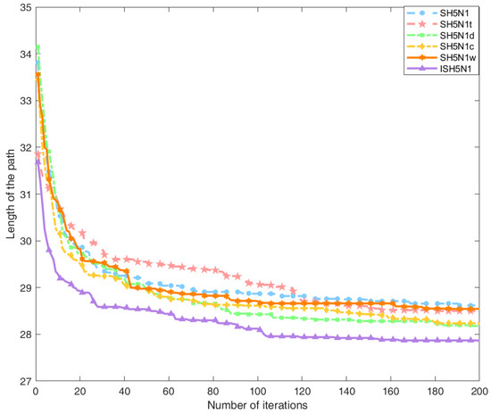
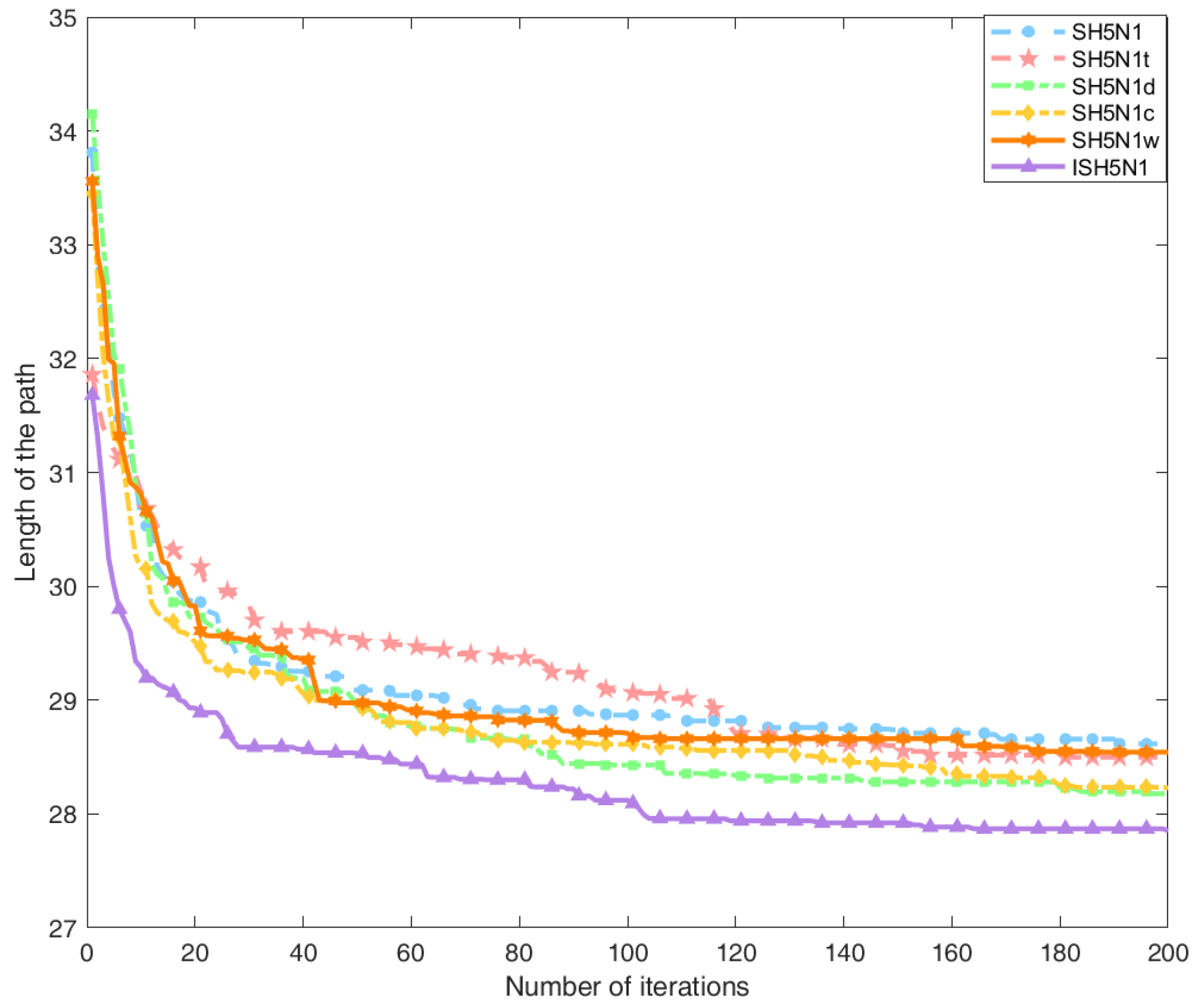
The effectiveness and superiority of ISH5N1 were validated in the simulation experiments of Section 5.2. To evaluate the efficacy of each improvement strategy—namely, the Tent chaotic map initial population, the position update strategy integrating multi-source directional information, the mutation step size control strategy enhanced by Logistic chaos, and the inertia weight decay coefficient wd optimization strategy—this study conducted a series of ablation experiments. Each mechanism was integrated with the original SH5N1 algorithm to create four extended variants, designated as SH5N1t, SH5N1d, SH5N1c, and SH5N1w, as shown in Table 6. A 20 × 20 grid map was used as the simulation environment, with each algorithm executed 10 times. The experimental results are presented in Table 7, while Figure 10 displays the convergence curves of the average path length for each algorithm in the ablation experiments.

Table 6. Algorithm and Integrated Mechanism.

Algorithm	Integrated Mechanism
SH5N1t	SH5N1 + Tent Chaos Initialization
SH5N1d	SH5N1 + Location Update Strategy Integrating Multi-Source Directional Information
SH5N1c	SH5N1 + Logistic Chaos-Enhanced Variable Step-Size Control Strategy
SH5N1w	SH5N1 + Optimization of Inertial Weight Decay Coefficient

Table 7. Comparison of algorithms.

Algorithm	Path Length			Number of Iterations
	Best	Mean	Std	Best	Mean	Std
SH5N1	27.5072	28.6165	0.73673	37	101.40	57.42
SH5N1t	27.5072	28.4986	0.90802	36	106.90	52.06
SH5N1d	27.5072	28.1779	0.87671	47	91.00	36.22
SH5N1c	27.5072	28.2275	0.63168	21	97.40	37.03
SH5N1w	27.5072	28.5427	0.48489	36	109.50	56.04
ISH5N1	27.5072	27.8525	0.49685	40	102.70	47.01

Figure 10. Ablation experiment convergence curve.

As shown in Figure 10, the improved ISH5N1 and SH5N1t exhibit significantly shorter path lengths than the original SH5N1 curve during the early iteration stages. This indicates that under the influence of Tent chaos initialization, ISH5N1 generates a higher-quality initial population that is closer to the global optimum, laying a solid foundation for subsequent convergence. SH5N1d demonstrates particularly outstanding convergence speed. Its curve approaches ISH5N1 after approximately 50 iterations and consistently maintains the lowest convergence rate among all single-mechanism algorithms. This indicates that the position update strategy, which integrates multi-source directional information, significantly enhances the algorithm’s global search capability. It effectively helps the population escape local optima and accelerates convergence toward the global optimum. Although SH5N1c, incorporating Logistic mutation step size control, exhibits slightly slower convergence than SH5N1d, it continuously refines solution quality during the mid-to-late stages. This results in a stable and smooth convergence curve, demonstrating strong local exploration capabilities. SH5N1t, which solely incorporates Tent chaos initialization, and SH5N1w, which only employs inertial weight decay coefficient optimization, did not demonstrate significant advantages over the baseline SH5N1 in convergence speed or final path length. The two curves in Figure 9 generally align closely with SH5N1. This occurs because Tent chaos primarily enhances early-stage search by increasing initial population diversity, while inertial weight decay primarily balances global exploration and local exploitation and suppresses oscillations. Neither alone can substantially boost performance, but both collectively improve algorithmic stability.

The statistical results in Table 7 further quantify the aforementioned phenomena. Compared to the baseline SH5N1, SH5N1d reduces the average path length from 28.6165 to 28.1779, achieving a 1.53% improvement, while simultaneously decreasing the average iteration count by approximately 10.26%. This demonstrates significant advantages in both optimization accuracy and convergence speed. SH5N1c exhibits a reduced average path length by approximately 1.36% and a slight decrease in average iterations, demonstrating good overall performance. Although SH5N1w shows only a marginal improvement of about 0.26% in average path length and an increase in average iterations, its path length standard deviation is as low as 0.48849, validating its role in enhancing algorithm stability. Compared to SH5N1, ISH5N1 achieves an average path length improvement of approximately 2.67% while maintaining similar average iterations and exhibiting smaller standard deviations for both path length and iterations.

In summary, the four strategies synergistically enhance the ISH5N1 algorithm: Tent chaos initialization provides a superior initial population; the position update strategy incorporating multi-source directional information accelerates convergence toward the global optimum; the logistic chaos-enhanced variable step size control strategy strengthens local search precision during the mid-to-late stages; and the inertia weight decay coefficient optimization strategy improves convergence smoothness and stability while preserving exploration capability. Through the synergistic effect of these strategies, ISH5N1 demonstrates superior performance in path planning problems compared to both single-strategy improved algorithms and the original algorithm, exhibiting excellent overall capabilities.

5.4. Scalability Analysis

To further validate the robustness of the algorithm on large-scale raster maps, this section scales the environment size to 50 × 50, 100 × 100, 150 × 150, 200 × 200, 250 × 250, 300 × 300 grid maps. Simulation comparisons were conducted between the proposed algorithm (ISH5N1) and DBO, BOA, WOA, and SH5N1. The results are presented in Table 8.

Table 8. Experimental Results.

Algorithm	Path Length in Different Environments
	50 × 50	100 × 100	150 × 150	200 × 200	250 × 250	300 × 300
DBO	91.8678	190.5013	293.3782	392.9866	493.7418	594.3651
BOA	93.6282	192.1421	287.7505	388.0416	485.1028	582.9876
WOA	90.7924	188.7524	284.9253	386.3662	483.4326	581.7221
SH5N1	86.9446	191.8678	292.7793	392.8836	495.8009	597.6738
ISH5N1	73.0266	164.1803	262.3749	367.8557	462.5298	560.7980

Overall, as the grid size increases, the path lengths of all algorithms exhibit near-linear growth, consistent with the complexity increase resulting from an expanded search space. However, across all scales, ISH5N1 consistently achieves the shortest path length, demonstrating its robust global optimization and path convergence capabilities even within larger search spaces. Taking the maximum scale of 300 × 300 as an example, ISH5N1 achieved a path length of 560.7980, significantly outperforming DBO (594.3651), BOA (582.9876), WOA (581.7221), and SH5N1 (597.6738). This demonstrates the method’s stable performance advantage even at extreme scales.

Building upon this foundation, to address the difficulty in determining whether advantages diminish with scale expansion based solely on absolute values, this paper further employs the “path length advantage” (relative advantage) presented in Table 9 to measure the extent of ISH5N1’s lead over each baseline algorithm. It can be observed that at 50 × 50, ISH5N1 holds advantages over DBO, BOA, WOA, and SH5N1 of 20.51%, 22.00%, 19.57%, and 16.01%, respectively. As the scale increases, this advantage generally shows a declining trend. At 300 × 300, it still maintains advantages of 5.65%, 3.81%, 3.60%, and 6.17%, respectively. This indicates that despite all methods facing greater search difficulty in large-scale scenarios, ISH5N1 can still maintain a considerable lead, demonstrating good large-scale applicability and engineering value.

Table 9. Length Advantage Comparison.

Algorithm	Path Length Advantage in Different Environments
	50 × 50	100 × 100	150 × 150	200 × 200	250 × 250	300 × 300
DBO	20.51%	13.82%	10.57%	6.39%	6.32%	5.65%
BOA	22.00%	14.55%	8.82%	5.20%	4.65%	3.81%
WOA	19.57%	13.02%	7.91%	4.79%	4.32%	3.60%
SH5N1	16.01%	14.43%	10.38%	6.37%	6.71%	6.17%

6. Conclusions

To address the issues of slow convergence, susceptibility to local optima, and unstable search processes in mobile robot path planning, this paper proposes an ISH5N1 optimization algorithm enhanced by multi-strategy fusion. First, the Tent chaos map is employed to generate the initial population, thereby improving its quality. Second, a position update strategy integrating multi-source directional information is introduced, enhancing search direction diversity and local cooperative convergence capabilities, thereby improving solution efficiency and accuracy. Building upon this, the mutation step size control factor c and inertia weight decay coefficient $w_d$ are optimized to achieve a better balance between exploration and exploitation, further strengthening the algorithm’s ability to escape local optima and enhance global exploration capabilities. Through simulation experiments on classical test functions and path planning simulations across three distinct grid map environments, comparative analysis was conducted against four other renowned intelligent optimization algorithms. Experimental results demonstrate that compared to the other four algorithms, the ISH5N1 exhibits higher convergence speed, solution accuracy, and stability, along with stronger global search capabilities and the ability to escape local optima. It also exhibits high stability and robustness in path planning tasks, with its optimization capability and adaptability outperforming the other four algorithms across diverse grid map environments. This validates its effectiveness and superiority in global path planning for mobile robots. Subsequent ablation experiments confirmed the efficacy of each improvement strategy in path planning. The ISH5N1’s high search efficiency and stability, coupled with its strong applicability and optimization capabilities, demonstrate its significant potential for practical applications.

In summary, this paper focuses on global path planning for mobile robots in grid maps, proposing a multi-strategy-enhanced ISH5N1 optimization algorithm that demonstrates excellent optimization performance. It provides innovative methods and insights for the research and application of mobile robot path planning. Although the proposed algorithm achieves favorable results, this study exclusively addresses global path planning for mobile robots in static environments. Future work will integrate dynamic window methods to explore the algorithm’s application in dynamic obstacle scenarios. Additional path evaluation metrics will be incorporated based on practical requirements, complemented by real-world experimental validation to enhance the algorithm’s practical applicability.

References

- Tang, Y.; Zakaria, M.A.; Younas, M. Path Planning Trends for Autonomous Mobile Robot Navigation: A Review. Sensors 2025, 25, 1206. [Google Scholar] [CrossRef] [Scilit]
- Lackner, T.; Hermann, J.; Kuhn, C.; Palm, D. Review of autonomous mobile robots in intralogistics: State-of-the-art, limitations and research gaps. Procedia CIRP 2024, 130, 930–935. [Google Scholar] [CrossRef] [Scilit]
- Ibrayev, S.; Ibrayeva, A.; Amanov, B.; Tolenov, S. Development of a Service Robot for Hospital Environments in Rehabilitation Medicine with LiDAR Based Simultaneous Localization and Mapping. arXiv 2024, arXiv:2411.04797. [Google Scholar] [CrossRef] [Scilit]
- Ren, X.; Huang, B.; Yin, H. A review of the large-scale application of autonomous mobility of agricultural platform. Comput. Electron. Agric. 2023, 206, 107628. [Google Scholar] [CrossRef] [Scilit]
- Pearson, E.; Mirisola, B.; Murphy, C.; Huang, C.; O’Leary, C.; Wong, F.; Meyerson, J.; Bonfim, L.; Zecca, M.; Spina, N.; et al. Robust Autonomous Mobile Manipulation for Substation Inspection. ASME J. Mech. Robot. 2024, 16, 115001. [Google Scholar] [CrossRef] [Scilit]
- Zhang, Y.; Li, Y.X.; Zhang, H.F.; Wang, Y. Earthshaker: A mobile rescue robot for emergencies and disasters through teleoperation and autonomous navigation. JUSTC 2023, 53, 4. [Google Scholar] [CrossRef] [Scilit]
- Choi, M.; Lee, S. Integration of Autonomous Robots in Environmental and Urban Planning. In Intelligent Moving Cities: Technological Leap and Social Integration of Autonomous Mobile Robots; Springer: Singapore, 2025. [Google Scholar]
- Badamasi, M.A.; Kabir, I.K.; Ahmed, G.; El-Ferik, S. Autonomous Mobile Robot Path Planning Techniques—A Review: Classical and Heuristic Techniques. IEEE Access 2025, 13, 117999–118022. [Google Scholar] [CrossRef] [Scilit]
- Zhang, L.; Cai, Z.; Yan, Y.; Yang, C.; Hu, Y. Multi-agent policy learning-based path planning for autonomous mobile robots. Eng. Appl. Artif. Intell. 2024, 129, 107631. [Google Scholar] [CrossRef] [Scilit]
- Zhang, Y.; Guo, Z.; Lu, Z.; Jiang, L.; Cao, H. Review of Path Planning Algorithms for Mobile Robots. Comput. Eng. Appl. 2026, 62, 26–39. [Google Scholar]
- Fu, X.; Huang, Z.; Zhang, G.; Wang, W.; Wang, J. Research on path planning of mobile robots based on improved A* algorithm. PeerJ Comput. Sci. 2025, 11, e2691. [Google Scholar] [CrossRef] [Scilit] [PubMed]
- Gu, Y.; Wang, Z.; Huang, Z. Energy-Efficient Path Planning for Snake Robots Using a Deep Reinforcement Learning-Enhanced A* Algorithm. Biomimetics 2025, 10, 826. [Google Scholar] [CrossRef] [Scilit] [PubMed]
- Li, X.; He, Q.; Yang, Q.; Wang, N.; Wu, H.; Yang, X. Research on an Optimal Path Planning Method Based on A* Algorithm for Multi-View Recognition. Algorithms 2022, 15, 171. [Google Scholar] [CrossRef] [Scilit]
- Ganesan, S.; Ramalingam, B.; Mohan, R.E. A hybrid sampling-based RRT* path planning algorithm for autonomous mobile robot navigation. Expert Syst. Appl. 2024, 258, 125206. [Google Scholar] [CrossRef] [Scilit]
- Yin, X.; Dong, W.; Wang, X.; Yu, Y.; Yao, D. Route planning of mobile robot based on improved RRT and TEB algorithm. Sci. Rep. 2024, 14, 8942. [Google Scholar] [CrossRef] [Scilit]
- Luo, Y.; Deng, J. Path Planning for Mobile Robots Based on Improved RRT-Connect and DWA Fusion. J. Syst. Simul. 2025, 37, 2545–2556. [Google Scholar]
- Jiang, W.; Liu, J.; Wang, W.; Wang, Y. Global Path Planning for Land–Air Amphibious Biomimetic Robot Based on Improved PPO. Biomimetics 2026, 11, 25. [Google Scholar] [CrossRef] [Scilit]
- Tao, B.; Kim, J.-H. Deep reinforcement learning-based local path planning in dynamic environments for mobile robot. J. King Saud Univ.-Comput. Inf. Sci. 2024, 36, 102254. [Google Scholar] [CrossRef] [Scilit]
- Hua, X.; Zhang, T.; Cao, J. Dynamic Path Planning for Vehicles Based on Causal State-Masking Deep Reinforcement Learning. Algorithms 2025, 18, 146. [Google Scholar] [CrossRef] [Scilit]
- Ab Wahab, M.N.; Nazir, A.; Khalil, A.; Ho, W.J.; Akbar, M.F.; Mohd Noor, M.H.; Mohamed, A.S.A. Improved genetic algorithm for mobile robot path planning in static environments. Expert Syst. Appl. 2024, 249, 123762. [Google Scholar] [CrossRef] [Scilit]
- Zhang, C.; Chen, C.; Lu, J.; Jing, X.; Liu, W. A Multi-Strategy Improved Zebra Optimization Algorithm for AGV Path Planning. Biomimetics 2025, 10, 660. [Google Scholar] [CrossRef] [Scilit] [PubMed]
- Ma, J.; Liu, Q.; Yang, Z.; Wang, B. Improved Trimming Ant Colony Optimization Algorithm for Mobile Robot Path Planning. Algorithms 2025, 18, 240. [Google Scholar] [CrossRef] [Scilit]
- Hason, F.; Al-Darraji, S. A review: On bio-inspired optimization methods for path planning of mobile robot. J. Intell. Comput. Inform. 2023, 2, 1–10. [Google Scholar] [CrossRef] [Scilit]
- Zhou, T.; Wei, W. Mobile robot path planning based on an improved ACO algorithm and path optimization. Multimed. Tools Appl. 2025, 84, 10899–10922. [Google Scholar] [CrossRef] [Scilit]
- Lou, T.-S.; Yue, Z.-P.; Jiao, Y.-Z.; He, Z.-D. A hybrid strategy-based GJO algorithm for robot path planning. Expert Syst. Appl. 2024, 238, 121975. [Google Scholar] [CrossRef] [Scilit]
- Feng, T.; Li, J.; Jiang, H.; Yang, S.X.; Wang, P.; Teng, Y.; Chen, S.; Fu, Q.; Luo, B. The Optimal Global Path Planning of Mobile Robot Based on Improved Hybrid Adaptive Genetic Algorithm in Different Tasks and Complex Road Environments. IEEE Access 2024, 12, 18400–18415. [Google Scholar] [CrossRef] [Scilit]
- Loganathan, A.; Ahmad, N.S. A Hybrid HHO-AVOA for Path Planning of a Differential Wheeled Mobile Robot in Static and Dynamic Environments. IEEE Access 2024, 12, 25967–25979. [Google Scholar] [CrossRef] [Scilit]
- Wang, Z.; Han, X.; Liang, S.; Liu, Z.; Gao, X. Mobile Robot Path Planning Based on Improved CPO Algorithm. In Proceedings of the 2025 5th International Conference on Mechanical, Electronics and Electrical and Automation Control (METMS), Chongqing, China, 9–11 May 2025; pp. 273–277. [Google Scholar]
- Xu, L.; Yuan, C.; Jiang, Z. Multi-Strategy Enhanced Secret Bird Optimization Algorithm for Solving Obstacle Avoidance Path Planning for Mobile Robots. Mathematics 2025, 13, 717. [Google Scholar] [CrossRef] [Scilit]
- Le, T.X.; Bui, T.T.; Tran, H.N. The H5N1 algorithm: A viral-inspired optimization for solving real-world engineering problems. Eng. Comput. 2025, 42, 1024–1096. [Google Scholar] [CrossRef] [Scilit]
- Xue, J.; Shen, B. Dung beetle optimizer: A new meta-heuristic algorithm for global optimization. J. Supercomput. 2023, 79, 7305–7336. [Google Scholar] [CrossRef] [Scilit]
- Mirjalili, S.; Lewis, A. The Whale Optimization Algorithm. Adv. Eng. Softw. 2016, 95, 51–67. [Google Scholar] [CrossRef] [Scilit]
- Arora, S.; Singh, S. Butterfly optimization algorithm: A novel approach for global optimization. Soft Comput. 2019, 23, 715–734. [Google Scholar] [CrossRef] [Scilit]
Disclaimer/Publisher’s Note: The statements, opinions and data contained in all publications are solely those of the individual author(s) and contributor(s) and not of MDPI and/or the editor(s). MDPI and/or the editor(s) disclaim responsibility for any injury to people or property resulting from any ideas, methods, instructions or products referred to in the content. |
© 2026 by the authors. Licensee MDPI, Basel, Switzerland. This article is an open access article distributed under the terms and conditions of the Creative Commons Attribution (CC BY) license.