Multi-Sensor Wharf Yard Settlement Forecasting via SSA-PCA Sensor Fusion and Heterogeneous Gradient Boosting

Abstract

Accurate prediction of wharf yard settlement is difficult because monitoring records combine long-term drift, nonlinear load responses, sensor noise, and redundant exogenous variables. This study presents a three-stage framework that integrates multi-sensor data, separates trend and residual components, and combines heterogeneous learners. An ARIMA model first extracts the linear settlement trend. Singular spectrum analysis then denoises temperature and stress signals, principal component analysis reduces their dimension, and explicit temporal encodings represent daily, weekly, and long-term patterns. A sliding window joins the historical residuals with the exogenous and temporal features. XGBoost, LightGBM, and CatBoost predict the residual correction on complementary feature subsets, with hyperparameters tuned independently for each library, and their out-of-fold predictions are combined by non-negative least squares (NNLS) weights estimated separately for each monitoring station. The trend and residual predictions are finally combined. Tests on 60 days of hourly data from 15 monitoring stations yield an MSE of 1.0098, and an R² of 0.9492. The method outperforms the LSTM, Prophet-XGBoost, and other evaluated baselines.

1. Introduction

Wharf yards are critical interfaces between marine and land transport. Their foundations are continuously affected by stacked cargo, environmental loads, and soil creep, which can produce spatially uneven settlement. Excessive deformation reduces operating efficiency and can cause serious hazards, including structural instability and deformation of gantry-crane rails. Accurate settlement prediction is therefore essential to structural safety [1] and is equally important for real-time condition monitoring and early warning in port yards. The purpose of settlement forecasting is to provide advance information on the potential evolution of wharf-yard deformation, rather than merely describe the current settlement state. Although continuous monitoring records reveal existing deformation, forecasting can help assess short-term settlement trends and identify periods that may warrant closer inspection. Settlement evolution is influenced by both its historical development and changes in environmental and loading conditions. Therefore, combining historical settlement measurements with temperature and stress observations may provide more comprehensive information for forecasting than relying on settlement history alone. The task remains difficult because settlement reflects coupled changes in temperature, stacking stress, and groundwater level, while long monitoring records often contain noise, gaps, and drift. Singular spectrum analysis (SSA) can separate weak components and reconstruct signals under strong noise [2], which makes it a useful basis for cleaning multi-source sensor data.

Engineering monitoring systems usually combine temperature, stress, and other sensors to capture different drivers of settlement. These exogenous signals contain noise, trends at several scales, and redundant information. Decomposition methods can separate a complex record into components that are modeled and fused separately, improving forecast accuracy [3,4]. Settlement itself also combines a slow linear trend caused by long-term soil creep with nonlinear fluctuations caused by daily thermal cycles and changes in stacking load. A single model seldom represents both components well. Hybrid models perform better because they can assign the linear and nonlinear patterns to different learners [5,6]. The central problem is thus to use multiple sensors effectively while separating components with different temporal behavior.

Existing hybrid methods leave three gaps. First, although combinations such as CNN-LSTM-ARIMA and ARIMA-LSTM improve complex time-series forecasts [7,8], their treatment of multi-sensor inputs often does not remove noise and redundancy systematically. Second, many methods add the outputs of separate models, such as a Prophet trend and an XGBoost residual forecast, without defining trend and residual estimation as distinct prediction tasks [9,10]. Third, residual correction often relies on one machine-learning model [11,12,13], which limits control over bias and variance in complex nonlinear mappings. A heterogeneous ensemble can reduce this dependence on a single learner.

This study addresses these gaps through coordinated preprocessing, feature construction, and modeling. SSA decomposes each temperature and stress signal into trend and periodic components and suppresses white noise. Principal component analysis (PCA), motivated by work that combines physical priors with data-driven displacement prediction [14], then reduces the cleaned exogenous variables to six components while limiting multicollinearity. ARIMA models the long-term linear trend at each station, whereas a separate nonlinear model corrects the residual. Historical residuals, exogenous principal components, and temporal encodings are joined in a sliding window. XGBoost, LightGBM, and CatBoost are trained on complementary feature subsets, with hyperparameters tuned independently for each library, and their chronological out-of-fold predictions are combined by non-negative least-squares weights estimated separately for each monitoring station.

Experiments use hourly records from 15 monitoring stations in a port yard. The proposed method achieves an RMSE of 0.9179 and an R² of 0.9492, outperforming SSA-ARIMA-LSTM [6], CNN-LSTM, Prophet-XGBoost [9], and a simplified DCM variational-inference baseline [15]. The ablation study further quantifies the contribution of each module and shows that the framework remains effective with a limited training set.

The remainder of this paper is organized as follows. Section 2 reviews related studies on settlement forecasting, multi-sensor fusion, and ensemble learning. Section 3 presents the proposed framework, including ARIMA-based trend and residual separation, SSA-PCA multi-sensor feature extraction, temporal encoding, feature selection, and heterogeneous gradient-boosting ensemble. Section 4 describes the dataset, evaluation metrics, and benchmark results. Section 5 discusses the ablation results, study limitations, and future research. Section 6 concludes the paper.

2. Related Work

Research on settlement forecasting follows three connected lines: deformation observation and geotechnical inference, monitoring-driven time-series models, and hybrid machine learning. Physical models represent consolidation and loading mechanisms but require site-specific parameters and repeated calibration. Data-driven models update more readily from monitoring records, yet their reliability depends on how they handle noise, cross-sensor dependence, and the coexistence of slow drift and short-term fluctuations.

2.1. Settlement Prediction for Reclaimed and Soft Ground

Port-yard development can cause long-term and spatially uneven settlement due to the consolidation of fill materials, compression of underlying soft soils, groundwater fluctuations, and construction loads acting over different time scales. Zhang et al. [16] combine time-series InSAR observations with an LSTM model for short-term subsidence prediction and a geotechnical model for long-term evolution in Tianjin Binhai New Area. Li et al. [17] use multi-temporal InSAR to map reclaimed-island deformation and combine sequential estimation with a geotechnical model to predict later settlement, while Ma et al. [18] apply grey-system modeling to ground settlement at a reclaimed airport. These studies show that a data-driven model can complement consolidation analysis. Their satellite sampling interval or regional spatial scale, however, differs from hourly monitoring at individual yard stations.

Field monitoring studies examine settlement at a finer operational scale. Chen et al. [19] compare random forest regression, multilayer perceptron, and XGBoost for total and uneven settlement of a soft-soil embankment under rolling dynamic compaction. The tree models perform better than the neural model when the monitoring sample is limited. Xu et al. [20] remove random measurement error before training a multi-input LSTM for dam settlement and include environmental variables to improve long-term prediction. Li et al. [21] use spatial-temporal relations among multiple dam monitoring points to reconstruct long missing settlement records. Together, these results show that noise control, environmental inputs, and information shared across sensors all affect prediction quality. They do not yet provide one pipeline that denoises several exogenous sensor families, removes their redundancy, and assigns the target trend and residual to different learners.

2.2. Decomposition and Hybrid Time-Series Forecasting

ARIMA remains useful when settlement contains a stable linear component, but a single ARIMA model cannot represent load-driven and environmental nonlinearities. Kouokam et al. [6] evaluate hybrid time-series models across financial and climatic indicators, while Rezaiy and Shabri [22] combine wavelet processing, ensemble empirical mode decomposition, and ARIMA for drought forecasting. Jin et al. [7] and Pierre et al. [8] further show that ARIMA can be combined with convolutional or recurrent networks. Freeman et al. [23] combine ARIMA and decision trees for attack detection, which provides evidence for joining linear and tree-based learners outside structural monitoring. These studies support decomposition and model combination, although most predict the original target with overlapping model roles rather than defining a trend forecast and a separate residual target.

Recent settlement studies use deeper decomposition-based architectures. Zou et al. [24] integrate SSA, CNN, LSTM, and a Transformer to predict settlement of buildings near shield tunnels from monitoring and construction variables. Xu et al. [20] instead emphasize random-error extraction and multi-input recurrence. Such networks can learn nonlinear temporal dependence, but their parameter count increases the risk of overfitting when only a short monitoring record is available. They also offer limited control over how redundant sensor channels enter the predictor. The present study therefore retains decomposition but uses PCA and gradient-boosting models to construct a more compact residual learner.

2.3. Multi-Sensor Fusion and Physics-Data Coupling

Multi-source monitoring can improve deformation prediction when each source contributes distinct information. Han et al. [25] combine fiber-optic settlement measurements with physical knowledge for dam foundations. Their framework uses dynamic Bayesian prediction during construction and an EEMD-PSO-SVR model during operation. These approaches strengthen physical interpretation or spatial coverage, but neither addresses redundancy among many correlated environmental channels with a unified reduction step.

Fusion also occurs at the measurement level. Fabris et al. [26] integrate InSAR and GNSS observations to calibrate and validate subsidence estimates over the Po River Delta. This combination improves spatial coverage and reference stability, but it focuses on deformation measurement rather than short-term forecasting. In a wharf yard, temperature and stress sensors record local drivers that are not represented directly by regional displacement products. Feature-level fusion is therefore more suitable for the present task. SSA first suppresses sensor noise, and groupwise PCA then converts the reconstructed temperature and stress components into a small set of complementary predictors.

2.4. Gradient Boosting and Stacked Ensembles

Gradient-boosting trees provide strong nonlinear regression with less training data than many deep networks. Chen and Guestrin [27] introduce XGBoost with regularization, sparse-data handling, and efficient approximate split search. Ke et al. [28] develop LightGBM with gradient-based one-side sampling and exclusive feature bundling for efficient learning from high-dimensional inputs. Prokhorenkova et al. [29] propose ordered boosting in CatBoost to reduce prediction shift. Their different tree construction rules create useful diversity even on a shared input space, and supplying each learner with a different feature subset enlarges this diversity.

Engineering studies often compare these learners separately. Huang et al. [11] and Tan et al. [12] demonstrate that tree ensembles capture nonlinear relations in multivariate environmental or geotechnical data, but they do not combine complementary tree models after time-series decomposition. Stacked generalization can learn a second-level model from out-of-fold predictions instead of selecting one base learner [30]. The framework in this study applies that principle only to the nonlinear settlement residual. It therefore preserves the ARIMA-based baseline component, limits sensor redundancy through SSA and PCA, and reduces dependence on the error pattern of any single tree model.

3. Methodology

3.1. Overall Framework

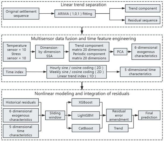
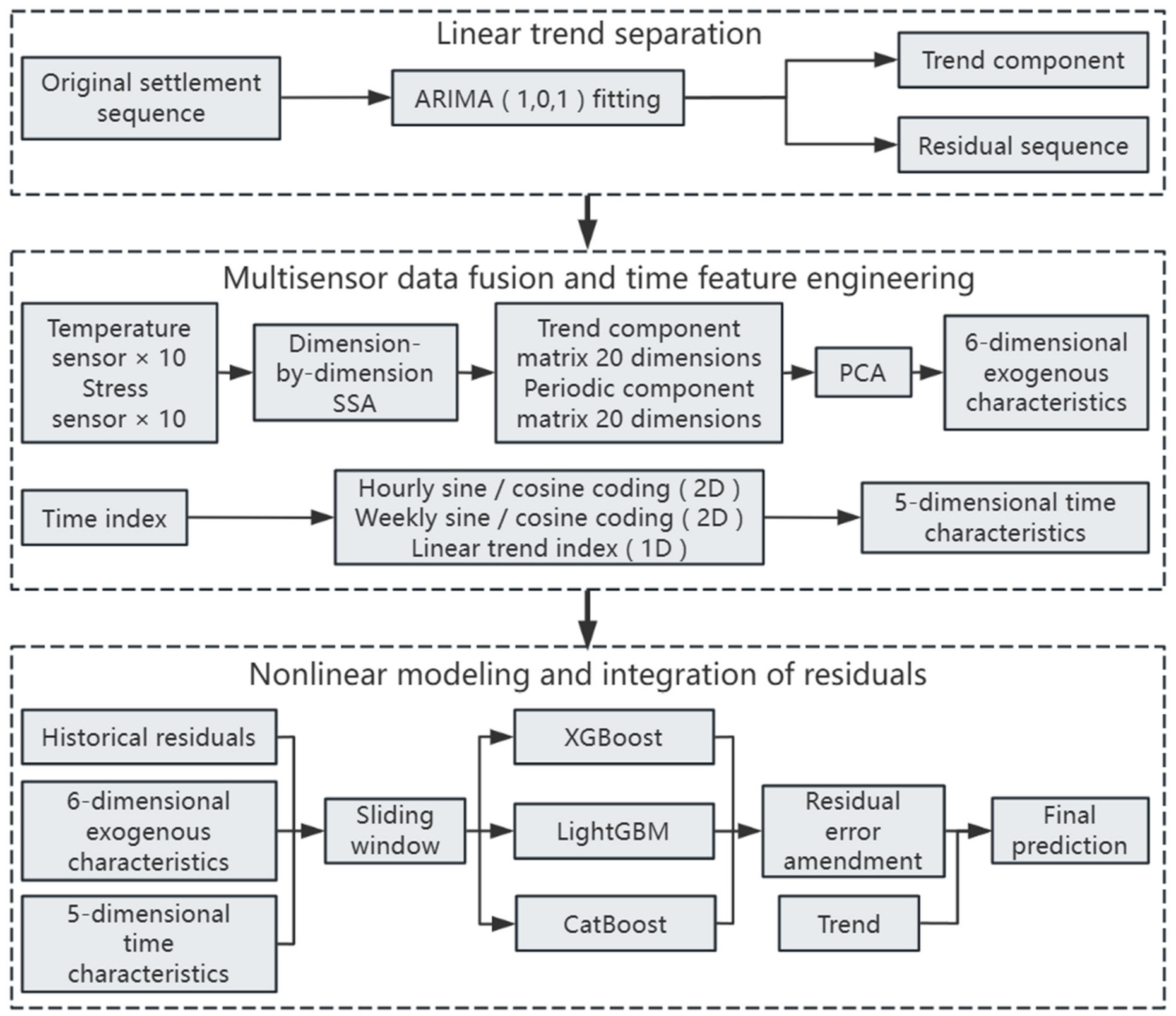
The proposed method uses the linear trend in settlement, the nonlinear effects recorded by multiple sensors, and temporal priors that represent periodicity and slow drift. The input contains 60 days of hourly data with 35 variables, comprising 15 settlement series, 10 temperature series, and 10 stress series. A 44-h sliding window provides the historical features, and the model generates rolling hourly forecasts for the following 12 days, corresponding to 288 h. Figure 1 summarizes the three-stage architecture.

Figure 1. Hybrid framework that combines ARIMA-based baseline component prediction with a heterogeneous tree ensemble for residual correction.

In the first stage, ARIMA fits the original settlement record and extracts a slowly varying trend $T_t$. The remaining sequence $r_t$ contains short-term fluctuations and nonlinear disturbances. This formulation treats trend prediction and nonlinear residual correction as separate tasks, allowing each component to use an appropriate model.

The second stage applies SSA independently to each temperature and stress signal, separates trend and periodic components, and removes white noise. PCA then compresses the cleaned exogenous variables to six dimensions while retaining at least 99% of their variance. Sine and cosine encodings of hour and weekday, together with a standardized linear time index, provide explicit periodic and long-term information.

The third stage flattens historical residuals, exogenous principal components, and temporal variables within the sliding window. After the flattened variables are ranked by XGBoost gain, complementary feature subsets are supplied to XGBoost, LightGBM, and CatBoost. Let their residual forecasts at time t be ${\widehat{r}}_t^{\mathit{XGB}}$, ${\widehat{r}}_t^{\mathit{LGB}}$, and ${\widehat{r}}_t^{\mathit{CAT}}$, respectively. Their out-of-fold predictions are combined by non-negative least squares into the weighted residual correction in Equation (1).

$${\widehat{r}}_t^{\mathit{ens}}=\left(w_1·{\widehat{r}}_t^{\mathit{XGB}}+w_2·{\widehat{r}}_t^{\mathit{LGB}}+{w_3·\widehat{r}}_t^{\mathit{CAT}}\right)$$

(1)

For each monitoring station, the non-negative weights $w_1$, $w_2$, and $w_3$ are estimated by non-negative least squares on the out-of-fold predictions of the three learners. The non-negativity constraint avoids cancellation between learners and makes each weight interpretable as that learner’s share of the correction. The ensemble correction is added to the trend estimate ${\widehat{y}}_t^{\mathit{trend}}$ from the first stage, which gives the final settlement forecast in Equation (2).

$${\widehat{y}}_t={\widehat{y}}_t^{\mathit{trend}}+{\widehat{r}}_t^{\mathit{ens}}$$

(2)

The architecture assigns the linear component to ARIMA, removes exogenous noise and redundancy with SSA and PCA, introduces known temporal structure through explicit encodings, and uses the heterogeneous tree ensemble to learn the remaining nonlinear response.

3.2. ARIMA-Based Trend Separation and Residual Modeling

Many ARIMA hybrids apply two models directly to the same original series, so their targets overlap and the linear and nonlinear components can interfere [6,7,8]. The proposed formulation instead separates the target into a trend forecast and a residual correction. For the hourly settlement sequence ${\left\{y_t\right\}}_{t=1}^N$, where $t$ is the time index, the ARIMA$\left(p,d,q\right)$ model is defined by Equation (3).

$$\left(1-{\displaystyle \sum _{i=1}^p}{\varphi }_i{B}^i\right)(1-B{)}^d{y}_t=\left(1+{\displaystyle \sum _{j=1}^q}{\theta }_j{B}^j\right){\epsilon }_t$$

(3)

Here, $\mathrm{B}$ is the lag operator and ${\epsilon }_t$ is white noise. An augmented Dickey-Fuller test indicates that the series is stationary, so $d = 0$. The Akaike information criterion is then minimized over $p\in [0,3], q\in [0,3]$, giving $p = 1, q = 1$ using the training data for each station independently. Maximum-likelihood estimation of ARIMA$\left(1,0,1\right)$ produces the fitted value ${\widehat{y}}_t^{\mathrm{ARIMA}}$, which is used as the trend $T_t$. To control the initial-point bias, the first $\max (p, q)$ trend values are set to the observations. The residual is then computed by Equation (4).

$$r_t={ y}_t-{ T}_t,t=1,2,\dots ,N$$

(4)

In Equation (4), $y_t$ is the observed settlement at time $t$, and $T_t$ is the trend estimated at the same time. Their difference $r_t$ contains the nonlinear and stochastic variation that the linear trend does not explain. This residual sequence becomes the target of the nonlinear ensemble. By learning only the unexplained component, the tree models avoid duplicating the linear structure already represented by ARIMA.

During testing, historical residual features are constructed using only settlement observations available at each forecasting origin. For each previously observed time step, the residual is calculated as the difference between the observed settlement and its corresponding ARIMA trend estimate. These historical residuals are then used as input features for the nonlinear forecasting model. Residuals associated with future, unobserved settlement values are not available at the current forecasting origin and are therefore excluded from the input features.

3.3. Exogenous Sensor Data Denoising Dimensionality Reduction and Temporal Encoding

Common preprocessing either standardizes exogenous sensors before direct input [11,12] or denoises one variable without a unified multivariate refinement stage. The proposed pipeline first decomposes each sensor with SSA, groups its trend and periodic components, and then compresses the groups separately with PCA.

3.3.1. SSA and Group Reconstruction

Temperature and stress records contain noise as well as variable-specific trends and cycles. Each exogenous sequence ${\left\{x_t\right\}}_{t=1}^N$ is therefore processed independently. With a window length $L = 24$ that matches the daily period, the method constructs the trajectory matrix $\mathit{X}\in R^{L\times K}$, where $K = N-L + 1$ and ${\mathit{X}}_{i,j} ={ x}_{i+j-1}$. Singular value decomposition gives $\mathit{X} = \mathit{U}\mathit{\Sigma }{\mathit{V}}^{\top }$, with singular values ${\mathrm{\sigma }}_1\ge { \mathrm{\sigma }}_2\ge \cdots \ge {\mathrm{\sigma }}_{\mathrm{L}}\ge 0$. The first component represents the trend, components two to four represent the periodic content, and the remaining components are treated as noise. Diagonal averaging maps the retained trajectory matrices back to time series.

Applying SSA to the 10 temperature and 10 stress sensors produces a trend matrix $\mathit{T}\in { R}^{N\times 20}$ and a periodic matrix $\mathit{C}\in { R}^{N\times 60}$. This group structure preserves the distinction between slow environmental drift and recurrent operating or thermal cycles before dimensionality reduction.

3.3.2. Group-Wise PCA and Temporal Encoding

Unlike the ARIMA-LSTM-SSA model [6], which directly supplies SSA outputs to the predictor, the proposed method applies PCA separately to $\mathit{T}$ and $\mathit{C}$. The first three principal components from each group explain at least 99% of the cumulative variance. They form the trend matrix ${\mathit{P}}_t\in { R}^{N\times 3}$ and periodic matrix ${\mathit{P}}_c\in { R}^{N\times 3}$, which are joined as the six-dimensional exogenous matrix $\mathit{P} = [{\mathit{P}}_t,{\mathit{P}}_c]\in R^{N\times 6}$. This group-wise compression reduces 40 SSA-derived variables to six while preserving the distinction between trend and periodic information.

The explicit temporal vector ${\mathit{c}}_t\in R^5$ contains five variables. Daily variation is represented by $\sin (2\pi h_t/24),\cos (2\pi h_t/24)$, where $h_t\in [0,23]$ is the hour of day. Weekly variation is represented by $\sin (2\pi w_t/7),\cos (2\pi w_t/7)$, where $w_t\in [0,6]$ identifies the weekday. The cumulative hourly index ${\mathit{idx}}_t$ represents slow drift from the start of training, including seasonal settlement or sensor aging. Z-score standardization produces ${\tilde{\mathit{c}}}_t$ on a scale consistent with the other inputs. These variables are joined with the reduced exogenous components and historical residuals before feature selection.

3.4. Feature-Importance Pruning and Heterogeneous Gradient-Boosting Ensemble

Residual correction with a single XGBoost, LSTM, or back-propagation model inherits the bias of that learner. The proposed model instead ranks the flattened features by cumulative XGBoost gain, supplies each of the three heterogeneous tree learners with a different nested subset of this ranking, and combines their out-of-fold predictions by non-negative least-squares weights estimated for each monitoring station. The nested subsets diversify the input spaces, while the weighted combination reduces dependence on any one model under limited sample size.

3.4.1. Sliding-Window Construction and Feature Selection

A window of $L = 44$ h joins historical residuals of size $L\times 15$, exogenous principal components of size $L\times 6$, and temporal encodings of size $L\times 5$. A 44-h window can provide a favorable balance between capturing two daily cycles and limiting dimensionality. Then, the input is flattened into the 1144-dimensional vector ${\mathit{x}}_t$, and the target is ${\widehat{r}}_{t+1}\in R^{15}$. Features are then ranked by cumulative XGBoost gain, and each learner receives a different prefix of this ranking: the full 1144-dimensional vector set for XGBoost, the 911-variable subset with 95% cumulative gain for CatBoost, and the 757-variable subset with 85% cumulative gain for LightGBM.

3.4.2. Heterogeneous Ensemble Prediction

Each monitoring station uses a chronological five-fold out-of-fold prediction scheme to avoid temporal information leakage. The training period was divided into five sequential folds. In each fold, the base learners were trained using only observations preceding the validation block and generated out-of-fold predictions for that block. The concatenated out-of-fold predictions of XGBoost, LightGBM, and CatBoost were then used to estimate the station-specific combination weights. The hyperparameters of the three libraries were tuned independently of one another. For each library, a library-specific search space covering tree depth, learning rate, the number of boosting rounds, row and column subsampling, and the regularization coefficients was explored on the temporally ordered validation subset, with early stopping on the validation loss selecting the number of rounds. XGBoost was tuned over its subsampling ratios and L1/L2 penalties, LightGBM over its number of leaves, feature fraction, and minimum child samples, and CatBoost over its depth and L2 leaf coefficient. Because the three libraries express capacity and regularization differently, their final configurations differ, and no hyperparameter value is shared across libraries.

All base learners minimize MSE. Their out-of-fold predictions form a three-dimensional meta-feature for every training sample. For each monitoring station, the weight vector ($w_1$, $w_2$, $w_3$) is estimated by non-negative least squares (NNLS), which minimizes the squared error between the observed residual and the weighted sum of the three out-of-fold predictions under the constraint that all weights are non-negative. The constraint prevents the learners from canceling one another and makes each weight interpretable as that learner’s share of the correction. The base learners are then retrained on all training samples, and their test predictions are combined with the same station-specific weights. This constrained linear combination requires no additional tunable hyperparameters [31].

The three models provide complementary inductive biases. LightGBM handles high-dimensional variables efficiently through histogram-based splitting, CatBoost is comparatively stable for skewed residuals, and XGBoost controls overall bias through regularization. Training the three learners on nested feature subsets further decorrelates their predictions and strengthens this complementarity. The ensemble further reduces RMSE from 0.9186 to 0.9179 and increases R² from 0.9491 to 0.9492, while the NRMSE remains at 7.20%.

4. Experiments and Results

4.1. Dataset and Preprocessing

The experimental data originate from a structural health monitoring system deployed in Area A of a Henan Zhoukou port yard. The data were collected continuously over two months (60 days) at an hourly sampling frequency, yielding 1440 valid time points. Settlement measurements from 15 monitoring stations (e.g., ZKG-WY-DC-05-North), expressed in millimeters (mm), serve as the target prediction variable, with a total of 60 × 24 × 15 = 21,600 settlement records after hourly alignment. Synchronous exogenous recordings include multiple sensor types related to yard environment and loading conditions, comprising 10 temperature sensors, 10 stress sensors, water-level gauges, and GNSS (Global Navigation Satellite System) receivers. The temperature and stress sensors are collocated with the settlement stations to capture environmental and load-induced effects on settlement. GNSS displacement measurements provide the historical information for settlement forecasting, while temperature and structural-response measurements provide complementary information on environmental and loading-related variations. The specifications and deployment information of selected sensors in the monitoring system are listed in Table 1.

Table 1. Specifications and deployment information of selected sensors in the monitoring system.

Data Type	Sensor Model and Manufacturer	Number and Configuration of Channels	Measurement Specifications and Deployment
Temperature	JTM-T4000 series thermometer, Jintumu, Zhongwei, China	10 channels	Measurement range: −30 to 120 °C; accuracy: ±0.5 °C.
Water level	JTM-WLD1000 radar water-level gauge, Jintumu	2 monitoring locations	Measurement range: 30 m/70 m; accuracy: ±3 mm/±10 mm. Installed at the third pile foundation from the waterfront at the upstream and downstream end bent frames of the wharf.
GNSS displacement	BGK-2850S GNSS receiver, GeoKang, Beijing, China	15 displacement-component series across five sites	Supports BDS and GPS. Each site records north, east, and vertical displacement components. All five sites are located within the yard area.
Structural response (recorded as “stress” in the dataset)	BGK4200 series vibrating-wire strain gauge, GeoKang	10 channels	Integrated temperature sensor; nominal strain range: 3000 με. The sensors are embedded in concrete at crossbeam midspans.

Sensor selection was guided by the relevance of each measurement to wharf-yard settlement forecasting and the availability of monitoring records. The engineering monitoring design considers sensor reliability, measurement accuracy, durability, and suitability for long-term automated operation. It specifies GNSS-based surface displacement monitoring, strain gauges for structural stress monitoring, and temperature–humidity sensors for environmental monitoring. Because the monitoring variables may have different sampling intervals, the available time series were aligned to an hourly grid during preprocessing. The statistical evaluation, including uncertainty estimates, paired daily error comparisons, daily prediction losses, and paired daily MSE differences can be found in the Appendix A Table A1, Table A2 and Table A3.

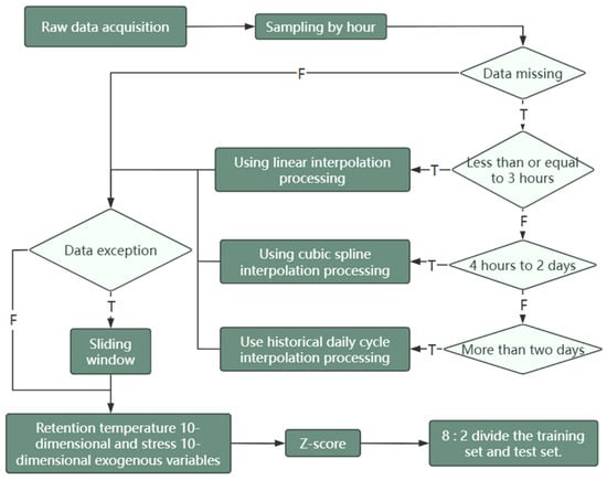
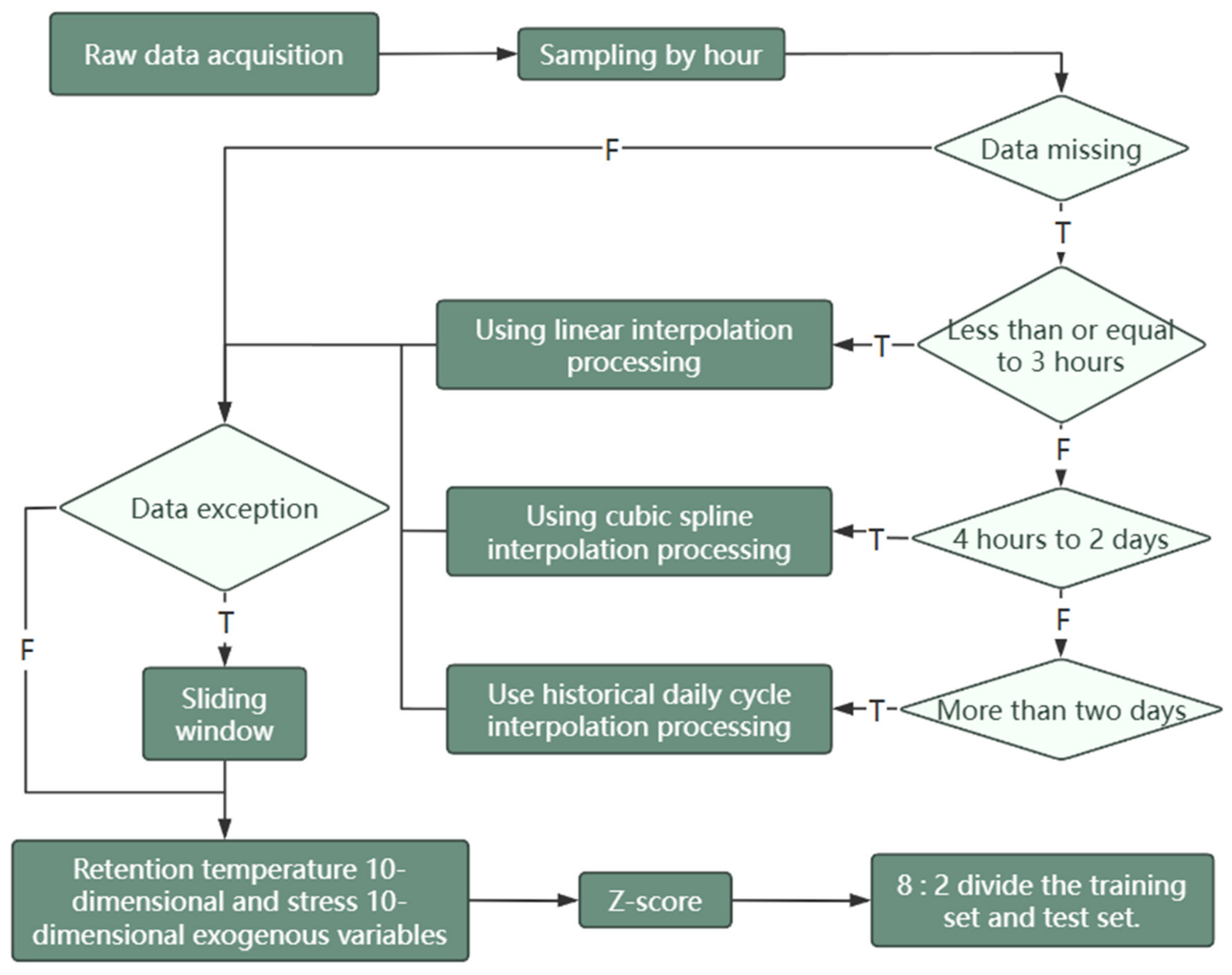
To identify the exogenous variables most strongly correlated with settlement, a systematic correlation analysis was conducted on all candidate variables of the training data. Temperature exhibits a maximum lagged correlation of 0.7788 with settlement at lag 0 h, a first canonical correlation coefficient of 0.8786 via canonical correlation analysis (CCA), and a maximum pairwise mutual information of 0.6381. Stress shows corresponding values of 0.8103, 0.8998, and 0.7333. These metrics confirm that both temperature and stress are significantly correlated with settlement in both linear and nonlinear senses. Accordingly, these two sensor types are selected as the final exogenous variables, yielding a 20-dimensional input (10 temperature + 10 stress). Other sensors, including water-level and pressure gauges, exhibit correlation coefficients below 0.3 with settlement and are excluded from the subsequent modeling. The overall preprocessing pipeline is summarized in Figure 2.

Figure 2. Data preprocessing pipeline (“T” means True, and “F” means False).

The original settlement series contains approximately 1.2% missing values and a small number of anomalies caused by communication interruptions or sensor faults. All series are first resampled to an hourly grid to ensure temporal alignment. A gap-length-dependent imputation strategy is applied: gaps of ≤3 h are filled by linear interpolation; gaps between 4 h and 48 h are filled by cubic spline interpolation to preserve local smoothness; and gaps exceeding 48 h are filled using historical daily periodic patterns, based on the historical mean of observations at the same hour from available preceding and following days. Residual missing values at the series boundaries are handled by forward or backward filling. For the validation and test periods, imputation is performed using only information available up to the corresponding forecasting time, thereby avoiding the use of future observations.

Anomaly detection is performed with a sliding window of 48 h (two complete daily cycles) applied to each monitoring station. Values exceeding the window mean ± 3 standard deviations are identified as anomalies and replaced by the window median. To prevent future-information leakage, the anomaly-detection statistics for each observation are calculated using only observations available up to that time. The anomaly rate across all stations is approximately 0.3%, primarily caused by instantaneous sensor jumps.

Given that temperature and stress have different units and ranges (temperature in °C, stress in MPa), all 20 exogenous variables are Z-score normalized to zero mean and unit variance to prevent scale effects during model training. The settlement series retains its original physical unit (mm) to preserve interpretability.

To ensure a leakage-free forecasting evaluation, the chronological train-test split was performed before any data-driven model fitting. The first 80% of the observations (approximately 1152 h, corresponding to the first 48 days) was designated as the training period, while the remaining 20% (approximately 288 h, corresponding to the final 12 days) was strictly reserved as the test period. Therefore, the forecasting horizon was defined as 12 days at hourly resolution, comprising 288 consecutive future time steps. A temporally ordered validation subset was further separated from the training period for hyperparameter tuning and early stopping.

All preprocessing operations involving estimated parameters were fitted exclusively using the training data. Specifically, the normalization statistics, SSA configuration parameters, PCA projection matrices, ARIMA parameters, feature-selection criteria, and model hyperparameters were derived only from the training period and subsequently fixed when processing the test periods. No test-period observations were used to estimate preprocessing parameters, select features, tune hyperparameters, or fit forecasting models.

After the above preprocessing steps, a complete, clean, and temporally aligned time-series dataset is obtained, comprising 15 settlement target variables and 20 exogenous feature variables, ready for subsequent modeling and prediction.

4.2. Evaluation Metrics

Performance is assessed with four regression metrics. Mean squared error (MSE) measures squared prediction error and assigns greater weight to large deviations, as defined in Equation (5).

$$\begin{array}{c}MSE={\displaystyle \frac{1}{ n}}{\displaystyle \sum _{i=1}^n}(y_i-{\widehat{y}}_i{)}^2\end{array}$$

(5)

In Equation (5), ${\mathrm{y}}_{\mathrm{i}}$ is the observed settlement, ${\widehat{\mathrm{y}}}_{\mathrm{i}}$ is the forecast, and $n$ is the number of test samples. Lower MSE indicates smaller overall prediction error. Root mean squared error (RMSE) is defined in Equation (6) and retains the physical unit of the target.

$$\begin{array}{c}RMSE=\sqrt{{\displaystyle \frac{1}{n}}{\displaystyle \sum _{i=1}^n}(y_i-{\widehat{y}}_i{)}^2}\end{array}$$

(6)

Lower RMSE indicates greater accuracy, and its sensitivity to long-tailed errors make it useful for detecting unstable forecasts. Normalized RMSE (NRMSE) divides RMSE by the observed range, as shown in Equation (7).

$$\begin{array}{c}NRMSE={\displaystyle \frac{\mathrm{RMSE}}{\mathit{max}\left(y\right)-\mathit{min}\left(y\right)}}\times 100\%\end{array}$$

(7)

Here, $\max \left(\mathrm{y}\right)$ and $\min \left(\mathrm{y}\right)$ are the maximum and minimum observed test values. NRMSE expresses relative error as a percentage and supports comparison across stations with different settlement ranges. The coefficient of determination R² measures the fraction of target variance explained by the model and is defined in Equation (8).

$$R^2=1-{\displaystyle \frac{{\displaystyle {\sum }_{i=1}^n}(y_i-{\widehat{y}}_i{)}^2}{{\displaystyle {\sum }_{i=1}^n}(y_i-\overline{y}{)}^2}}$$

(8)

In Equation (8), $\overline{y}$ is the mean of the observations. A value of ${\mathrm{R}}^2$ near one indicates a close fit, whereas a value near zero indicates little predictive power.

4.3. Benchmark Comparison

Four representative baselines test the proposed method. The simplified DCM variational-inference baseline [15] is a simplified ADVI Bayesian regression that omits the causal estimator and structural causal model of the original MCST framework. It applies SSA and six-dimensional PCA to the exogenous data, expands them into 27 nonlinear variables, fits Bayesian linear regression to standardized settlement, models each station independently, and draws 2000 posterior samples. The CNN + LSTM baseline uses a one-dimensional convolution with kernel size 3 and 32 filters, pooling with stride 2, and two LSTM layers with 64 hidden units each. All models use a 44-h input window. The performance comparison with additional simple model baselines is presented in Appendix B (Table A4).

Prophet-XGBoost [9] decomposes the original settlement series into trend, periodic, and residual components with default Prophet settings. XGBoost predicts the residual from the supplied exogenous variables, and the three components are recombined. The reproduced SSA-ARIMA-LSTM model [6] decomposes settlement and temperature with SSA, reduces temperature trend, temperature cycle, and stress variables by K-means into three clusters per group, and joins 44 autoregressive lags with sine and cosine time encodings to form a 688-dimensional input. A single LSTM layer with 64 hidden units predicts 15 residuals from an ARIMA (1,0,1) fit to the SSA trend. All baselines use the same chronological split and window length as the proposed method.

Table 2 summarizes the prediction performance of the proposed method and four baseline models. The proposed method achieves an MSE of 1.0098, an RMSE of 0.9179, an NRMSE of 7.20%, and an R² of 0.9492. Among the four baselines, the simplified DCM variational-inference model obtains the lowest performance, with an RMSE of 2.6948 and an R² of 0.5634. The CNN + LSTM model improves the prediction accuracy, achieving an RMSE of 1.4746 and an R² of 0.8771. Prophet-XGBoost further reduces the RMSE to 1.1913 and increases R² to 0.9175, while SSA-ARIMA-LSTM achieves an RMSE of 1.1477 and an R² of 0.9215.

Table 2. Prediction performance of the evaluated models.

Model	MSE	RMSE	NRMSE	R2
simplified DCM variational inference [15]	8.6751	2.6948	21.05%	0.5634
CNN + LSTM	2.4428	1.4746	11.90%	0.8771
Prophet-XGBoost [9]	1.6386	1.1913	9.48%	0.9175
SSA-ARIMA-LSTM [6]	1.5608	1.1477	9.05%	0.9215
Proposed method	1.0098	0.9179	7.20%	0.9492

Note: The best results for each evaluation metric are highlighted in bold.

To further examine the variation in forecasting performance across monitoring series, the station-level results are reported in Table 3. These results indicate that the proposed model performs less favorably for several series with relatively larger prediction errors, although the available monitoring records do not provide sufficient field information to attribute these differences to specific physical causes.

Table 3. Station-level forecasting performance of the proposed method.

Monitoring Series	MSE	RMSE	MAE	NRMSE	R2
ZKG-WY-DC-05-North	0.6309	0.7943	0.5051	5.96%	0.8679
ZKG-WY-DC-06-East	0.2780	0.5272	0.3149	6.45%	0.9006
ZKG-WY-DC-07-East	0.3701	0.6084	0.3589	8.72%	0.8075
ZKG-WY-DC-04-Gao	1.7779	1.3334	0.7766	8.54%	0.8213
ZKG-WY-DC-05-Gao	1.9422	1.3936	0.8578	8.40%	0.8621
ZKG-WY-DC-04-East	0.2435	0.4935	0.3142	5.83%	0.9134
ZKG-WY-DC-06-North	0.9685	0.9841	0.5842	9.00%	0.8055
ZKG-WY-DC-08-North	0.5580	0.7470	0.4807	7.29%	0.8551
ZKG-WY-DC-05-East	0.2011	0.4484	0.2888	5.10%	0.9363
ZKG-WY-DC-07-Gao	3.2200	1.7944	0.9584	8.91%	0.7854
ZKG-WY-DC-08-Gao	1.4987	1.2242	0.7328	6.76%	0.8583
ZKG-WY-DC-06-Gao	2.0858	1.4442	0.8616	6.87%	0.8368
ZKG-WY-DC-07-North	0.6935	0.8328	0.5198	6.42%	0.8231
ZKG-WY-DC-08-East	0.2106	0.4589	0.2926	6.51%	0.8884
ZKG-WY-DC-04-North	0.4689	0.6848	0.4259	7.19%	0.8202
Mean across series	1.0098	0.9179	0.5515	7.20%	0.8521

Note: the arithmetic mean of the 15 stations’ R² values is 0.8521, whereas the pooled R² of the proposed method is 0.9492.

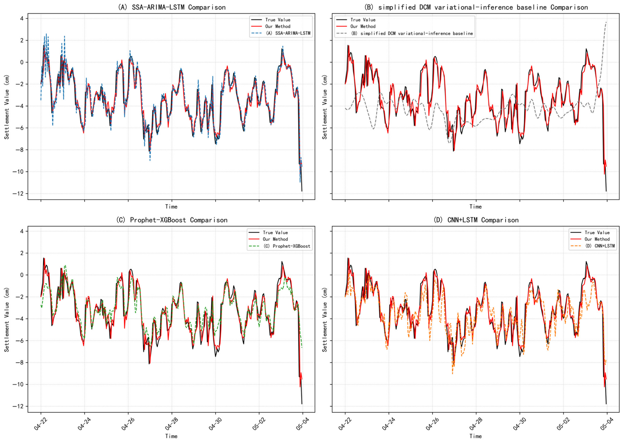
Figure 3 compares the predicted test curves. The black line is the observed settlement, the red line is the proposed forecast, and the dashed line in each panel is the corresponding baseline. Each panel isolates one baseline so that local fit and large deviations remain visible.

Figure 3. Predicted settlement curves for the proposed method and four baselines at station ZKG-WY-DC-05-North: (A) SSA-ARIMA-LSTM; (B) simplified DCM variational inference; (C) Prophet-XGBoost; (D) CNN + LSTM.

Compared with SSA-ARIMA-LSTM, the proposed method reduces the RMSE from 1.1477 to 0.9179 and the NRMSE from 9.05% to 7.20%, while increasing R² from 0.9215 to 0.9492. This improvement is obtained through the combination of residual autoregressive modeling, SSA-PCA-based exogenous feature extraction, temporal encoding, feature selection, and heterogeneous gradient-boosting ensemble learning. Specifically, the proposed framework replaces the K-means-based feature construction used in SSA-ARIMA-LSTM with six PCA components, constructs a 44-h historical feature window, and trains XGBoost, LightGBM, and CatBoost on complementary feature subsets. Their predictions are subsequently combined using station-specific non-negative least-squares weights learned from chronological out-of-fold (OOF) predictions.

Figure 3 further compares the predicted settlement curves of the proposed method with the four baseline models at station ZKG-WY-DC-05-North. The black line represents the observed settlement, the red line represents the proposed forecast, and the dashed line represents the corresponding baseline prediction. The results show that the proposed method generally follows the observed settlement trend more closely and reduces large deviations during the test period.

Compared with Prophet-XGBoost, the proposed method improves R² from 0.9175 to 0.9492 and reduces NRMSE from 9.48% to 7.20%. This improvement suggests that explicitly separating the settlement trend and residual components, together with SSA-PCA-based processing of the exogenous variables, can provide more effective inputs for nonlinear residual prediction. The heterogeneous ensemble further combines the complementary prediction characteristics of the three gradient-boosting models.

Overall, the results in Table 2 demonstrate that the proposed framework provides consistent improvements over all four evaluated baselines in terms of MSE, RMSE, NRMSE, and R². The results also support the effectiveness of combining multi-sensor feature extraction, residual modeling, and heterogeneous ensemble learning for short-term wharf-yard settlement forecasting.

4.4. Impact of Historical Window Length on Forecasting Performance

The historical window length (L) determines the amount of historical information used for settlement forecasting. In practical wharf-yard monitoring, the selection of a historical window should consider not only prediction accuracy but also engineering requirements, including the continuity of settlement trend assessment, the timeliness of forecasting, and the computational cost of processing monitoring data. A window that is too short may not provide sufficient temporal context for interpreting settlement variations, whereas a substantially longer window increases the input dimensionality and model complexity without necessarily improving prediction accuracy.

Considering these engineering requirements and the limited duration of the available monitoring dataset, a 44 h historical window was initially adopted as a practical compromise. To examine the sensitivity of the forecasting performance to this choice, we further evaluated window lengths of 48, 72, and 96 h while keeping the other experimental settings unchanged.

As shown in Table 4, the test mean RMSE values for the four window lengths range from 0.9165 to 0.9186, indicating relatively small variations in predictive performance. The 72 h window achieves the lowest RMSE of 0.9165, compared with 0.9179 for the 44 h window, corresponding to an absolute difference of only 0.0014. However, the 72 h window increases the input dimensionality from 1144 to 1872. From an engineering application perspective, the 44 h window therefore provides a reasonable balance between predictive accuracy, historical context, and input complexity, while avoiding the additional computational burden associated with longer windows. Accordingly, we retain 44 h as the default configuration for subsequent experiments.

Table 4. Sensitivity Analysis of Historical Window Length.

History Window (h)	Training Samples	Input Dimension	Test Mean RMSE
44	1108	1144	0.9179
48	1104	1248	0.9186
72	1080	1872	0.9165
96	1056	2496	0.9182

5. Discussion

5.1. Ablation Study

A cumulative ablation study measures the contribution of each module. Every variant uses the same training and test split, the same 44-h window, and the same MSE, RMSE, NRMSE, and R² metrics. Table 5 reports the results.

Table 5. Results of the cumulative ablation study.

Model Variant	MSE	RMSE	NRMSE	R2
ARIMA baseline	1.3475	1.0615	8.33%	0.9322
+ XGBoost residual correction	1.0223	0.9241	7.25%	0.9485
+ SSA-PCA exogenous features	1.0131	0.9198	7.21%	0.9490
+ temporal features	1.0112	0.9186	7.20%	0.9491
+ ensemble module	1.0098	0.9179	7.20%	0.9492

Note: The “+” symbol indicates the sequential addition of the corresponding component to the preceding model configuration. The best results for each evaluation metric are highlighted in bold.

ARIMA alone reaches MSE = 1.3475 and R² = 0.9322, indicating that linear temporal structure accounts for much of the predictable settlement variation in this dataset. Adding XGBoost residual correction raises R² to 0.9485 and reduces NRMSE to 7.25%. MSE falls from 1.3475 to 1.0223, which is the largest improvement between consecutive variants. This result supports assigning the remaining predictive structure to a separate nonlinear learner. Historical residuals provide information about recent deviations from the ARIMA estimate, allowing the correction model to target errors that persist after linear modeling.

Adding the SSA-PCA temperature and stress components further increases R² to 0.9490 and lowers NRMSE to 7.21%. The smaller gain suggests that these variables supplement information already present in the residual history. SSA reconstruction and groupwise PCA provide a compact representation of environmental and loading signals, with the 40 reconstructed trend and periodic variables reduced to six components. Explicit temporal encodings then raise R² to 0.9491 and reduce NRMSE to 7.20%. Their limited additional benefit is consistent with partial overlap between the encoded cycles and the temporal information available through the 44-h window and reconstructed sensor components. As reported in Appendix C (Table A5), the 24 h SSA embedding length and three-component-per-group PCA setting achieved the lowest test mean RMSE among the evaluated configurations.

The heterogeneous stacking module produces the final R² of 0.9492, RMSE of 0.9179, and NRMSE of 7.20%. Relative to the preceding variant, MSE decreases from 1.0112 to 1.0098. This modest improvement is consistent with the ensemble exploiting differences among the three base learners. The station-specific non-negative least-squares weights combine their out-of-fold residual predictions without negative coefficients, providing a controlled way to refine the correction after the main temporal and exogenous information has been incorporated.

Across the full sequence, RMSE decreases from 1.0615 to 0.9179, corresponding to a relative reduction of 14%. Residual correction accounts for most of the gain, while the later modules provide incremental refinement. These results suggest that the roles of the modules are complementary rather than additive in terms of accuracy alone. Although the numerical improvements of these later modules are modest, they contribute to the overall design by improving feature representation and reducing dependence on a single predictive model.

5.2. Limitations and Future Work

The present evaluation has several limits. The dataset covers 60 consecutive days at 15 stations in one area of a single port-yard, and the final 12 days form the only held-out test period. The reported performance therefore characterizes short-term prediction under the observed loading and environmental conditions. It does not establish seasonal stability, transfer to other ports, or reliability during rare events such as abrupt loading changes, prolonged sensor outages, or extreme weather. Longer records from several yards and external validation across different loading regimes are needed before the model is used as a general forecasting tool. The relatively short monitoring duration also limits the amount of independent temporal information available for machine-learning training. Although the dataset contains 1152 hourly observations per station in the training period, it does not cover different seasons, long-term changes in loading conditions, or rare environmental events. To mitigate overfitting under this limited-data setting, PCA-based dimensionality reduction and chronological out-of-fold training were adopted.

Several modeling choices are fixed from the current dataset. SSA uses a daily window, the supervised model uses a 44-h history, and ARIMA parameters are estimated exclusively using the training period and were not re-estimated using test observations. These choices may become suboptimal when operating cycles or settlement trends change. From a methodological perspective, this study demonstrates the feasibility of integrating trend-residual decomposition, SSA-PCA-based multi-sensor feature extraction, and heterogeneous gradient boosting for wharf-yard settlement forecasting. The ablation results indicate that nonlinear residual correction accounts for most of the observed improvement, while the incorporation of exogenous sensor features and ensemble learning provides additional, but relatively modest, gains. These findings highlight the importance of evaluating the contribution of each component when developing forecasting frameworks for practical monitoring scenarios. However, the current evaluation is based on 60 days of data from a single yard area. Future work will therefore focus on validating the framework using longer monitoring records and data from independent sites to assess its generalizability.

The current framework predicts each station independently and provides point forecasts. Future work can model spatial dependence through graph-based or multi-task learning so that nearby stations share information without removing local behavior. Prediction intervals and calibrated uncertainty estimates are also required for warning decisions, particularly when measurements are missing or the input distribution shifts. A practical extension is an incremental monitoring system that detects drift, updates the model when new data arrive, and reports both the forecast and its uncertainty.

6. Conclusions

This study presents a wharf yard settlement forecasting framework that combines SSA decomposition, PCA reduction, ARIMA trend extraction, explicit temporal encoding, and heterogeneous tree stacking. SSA separates trend and periodic components in the exogenous sensors, and PCA converts them into compact features. Modeling the ARIMA residual instead of the original series assigns the linear and nonlinear components to different learners. XGBoost, LightGBM, and CatBoost, each trained on a different feature subset with independently tuned hyperparameters, are combined by per-station non-negative least-squares weights, which further improves accuracy and stability. Finally, OOF-based station-specific NNLS weighting is introduced to adaptively combine the predictions of different gradient boosting models. On the 15-station dataset, the method attains MSE = 1.0098, RMSE = 0.9179, R² = 0.9492 and NRMSE = 7.20%, outperforming the evaluated LSTM and Prophet-XGBoost baselines under a limited sample size.

Appendix A.1. Statistical Evaluation

This appendix reports the uncertainty procedure and daily losses underlying the comparisons with SSA-ARIMA-LSTM, CNN + LSTM, simplified DCM variational inference and Prophet-XGBoost. All supplementary analyses follow the same experimental workflow as in the original study. The evaluation contains 288 hourly test observations from 22 April to 3 May 2026 for 15 monitoring series.

Appendix A.1.1. Evaluation Units and Uncertainty Estimates

Mean RMSE is calculated by first computing RMSE separately for each of the 15-monitoring series and then taking their arithmetic mean. Each daily MSE averages 360 squared errors: 24 h multiplied by 15 series. Daily MSE and mean series-specific RMSE therefore use different aggregation orders.

Nominal 95% percentile confidence intervals are estimated using 2000 paired moving-block bootstrap resamples with 24 h blocks. Common time indices are used across models and monitoring series, retaining their alignment within each sampled block. The baseline and proposed method are compared within the same resample. These intervals describe uncertainty conditional on the fitted workflows and available test record; they do not quantify variation from repeated model training. The block length does not guarantee that dependence at longer lags is captured.

For the Wilcoxon comparisons, the paired difference is baseline daily MSE minus proposed daily MSE. There are 12 daily differences per baseline. All are positive, with positive and negative rank sums of 78 and 0. Thus W = 0 and the exact two-sided p value under the signed-rank null assumptions is 2/4096 = 0.00048828125. Holm adjustment within this family of four comparisons gives 0.001953125. Identical p values reflect the common all-positive rank pattern, while the effect magnitudes differ.

The standard deviations (SDs) in Table A1, Table A2 and Table A3 are sample SDs across the 12 test days, using denominator 11. They do not represent cross-validation or repeated-fit variability. Daily aggregation does not establish independence between consecutive differences. The signed-rank results rely on the independence and symmetry assumptions and are treated as supplementary to the paired effect estimates.

Table A1. Paired daily error comparisons.

Baseline Model	Daily MSE Difference Mean ± SD	Days Won/Lost (12 Days)	Series Won/Lost (15 Series)	W	Unadjusted p	Holm-Adjusted p
SSA-ARIMA-LSTM [6]	0.5510 ± 0.3591	12 0	15/0	0	0.000488	0.001953
CNN + LSTM	1.4330 ± 0.3316	12/0	15/0	0	0.000488	0.001953
simplified DCM variational inference [15]	7.6653 ± 3.9394	12/0	15/0	0	0.000488	0.001953
Prophet-XGBoost [9]	0.6288 ± 0.2291	12/0	15/0	0	0.000488	0.001953

Note: Positive differences favor the proposed method. Day counts compare daily MSE over 12 dates; series counts compare each series-specific RMSE over all 288 test hours. Counts are from the proposed method’s perspective. CIs and p values concern different summaries of the prediction errors.

Table A1. Paired daily error comparisons.

Baseline Model	Daily MSE Difference Mean ± SD	Days Won/Lost (12 Days)	Series Won/Lost (15 Series)	W	Unadjusted p	Holm-Adjusted p
SSA-ARIMA-LSTM [6]	0.5510 ± 0.3591	12 0	15/0	0	0.000488	0.001953
CNN + LSTM	1.4330 ± 0.3316	12/0	15/0	0	0.000488	0.001953
simplified DCM variational inference [15]	7.6653 ± 3.9394	12/0	15/0	0	0.000488	0.001953
Prophet-XGBoost [9]	0.6288 ± 0.2291	12/0	15/0	0	0.000488	0.001953

Note: Positive differences favor the proposed method. Day counts compare daily MSE over 12 dates; series counts compare each series-specific RMSE over all 288 test hours. Counts are from the proposed method’s perspective. CIs and p values concern different summaries of the prediction errors.

Appendix A.1.2. Daily Prediction Losses

Table A2 gives the complete daily MSE values used to describe error variation during the test interval. Each entry is the average squared error over the same 24 h and 15 monitoring series. The last row reports the mean and sample SD across the 12 dates.

Table A2. Daily mean squared errors.

Date	Proposed Method	SSA-ARIMA-LSTM [6]	CNN + LSTM	Simplified DCM Variational Inference [15]	Prophet-XGBoost [9]
22 April 2026	1.0307	2.3522	2.7411	17.1734	1.7997
23 April 2026	0.9316	1.6338	1.9581	14.6864	1.4998
24 April 2026	1.3492	2.4172	2.4138	6.5948	1.9112
25 April 2026	0.9608	1.2665	2.7595	6.7789	1.7998
26 April 2026	0.9242	1.4682	2.6187	6.3740	1.3971
27 April 2026	1.6683	2.4886	2.8788	7.6145	2.0794
28 April 2026	0.5949	0.7895	1.6650	4.9171	0.9739
29 April 2026	0.8038	1.1028	2.1017	5.2764	1.2337
30 April 2026	1.0595	1.5488	2.6533	9.4530	2.1337
1 May 2026	0.9423	1.2613	2.1186	5.9140	1.6250
2 May 2026	0.8829	1.1715	2.4340	7.0476	1.3114
3 May 2026	0.9699	1.2293	2.9722	12.2717	1.8987
Mean ± SD	1.0098 ± 0.2704	1.5608 ± 0.5622	2.4429 ± 0.4042	8.6752 ± 3.9564	1.6386 ± 0.3598

Note: The daily means and SDs are calculated across the 12 test days. Values are rounded for display.

Table A2. Daily mean squared errors.

Date	Proposed Method	SSA-ARIMA-LSTM [6]	CNN + LSTM	Simplified DCM Variational Inference [15]	Prophet-XGBoost [9]
22 April 2026	1.0307	2.3522	2.7411	17.1734	1.7997
23 April 2026	0.9316	1.6338	1.9581	14.6864	1.4998
24 April 2026	1.3492	2.4172	2.4138	6.5948	1.9112
25 April 2026	0.9608	1.2665	2.7595	6.7789	1.7998
26 April 2026	0.9242	1.4682	2.6187	6.3740	1.3971
27 April 2026	1.6683	2.4886	2.8788	7.6145	2.0794
28 April 2026	0.5949	0.7895	1.6650	4.9171	0.9739
29 April 2026	0.8038	1.1028	2.1017	5.2764	1.2337
30 April 2026	1.0595	1.5488	2.6533	9.4530	2.1337
1 May 2026	0.9423	1.2613	2.1186	5.9140	1.6250
2 May 2026	0.8829	1.1715	2.4340	7.0476	1.3114
3 May 2026	0.9699	1.2293	2.9722	12.2717	1.8987
Mean ± SD	1.0098 ± 0.2704	1.5608 ± 0.5622	2.4429 ± 0.4042	8.6752 ± 3.9564	1.6386 ± 0.3598

Note: The daily means and SDs are calculated across the 12 test days. Values are rounded for display.

The arithmetic mean of the daily MSEs is comparable to an equally weighted mean of series-specific MSEs because every date contains the same number of hours and series. Taking its square root, however, is not equivalent to averaging the 15 series-specific RMSE values. This distinction explains why the reported mean RMSE is not required to equal the square root of the reported mean MSE.

Appendix A.1.3. Paired Daily Differences

Table A3 reports baseline daily MSE minus proposed daily MSE on each date. These differences form the 12 paired observations for each signed-rank comparison. Every displayed daily difference is positive.

Table A3. Paired daily MSE differences.

Date	SSA-ARIMA-LSTM [6]	CNN + LSTM	Simplified DCM Variational Inference [15]	Prophet-XGBoost [9]
22 April 2026	1.321495	1.710392	16.142660	0.769004
23 April 2026	0.702140	1.026458	13.754816	0.568162
24 April 2026	1.068016	1.064620	5.245595	0.562036
25 April 2026	0.305615	1.798669	5.818074	0.838912
26 April 2026	0.544028	1.694466	5.449799	0.472914
27 April 2026	0.820239	1.210494	5.946169	0.411038
28 April 2026	0.194605	1.070078	4.322213	0.379008
29 April 2026	0.298985	1.297846	4.472539	0.429809
30 April 2026	0.489303	1.593798	8.393567	1.074229
1 May 2026	0.319041	1.176352	4.971744	0.682679
2 May 2026	0.288618	1.551061	6.164657	0.428445
3 May 2026	0.259435	2.002309	11.301872	0.928855
Mean difference	0.550960	1.433045	7.665309	0.628758
SD of differences	0.359110	0.331562	3.939440	0.229057
Positive/negative/zero	12/0/0	12/0/0	12/0/0	12/0/0

Note: Daily differences retain six decimal places and use losses before display rounding. Subtracting the four-decimal entries in Table A2 can therefore produce a small discrepancy. For example, on 22 April, the SSA-ARIMA-LSTM difference is 2.352197 − 1.030702 = 1.321495. SD uses denominator 11.

Table A3. Paired daily MSE differences.

Date	SSA-ARIMA-LSTM [6]	CNN + LSTM	Simplified DCM Variational Inference [15]	Prophet-XGBoost [9]
22 April 2026	1.321495	1.710392	16.142660	0.769004
23 April 2026	0.702140	1.026458	13.754816	0.568162
24 April 2026	1.068016	1.064620	5.245595	0.562036
25 April 2026	0.305615	1.798669	5.818074	0.838912
26 April 2026	0.544028	1.694466	5.449799	0.472914
27 April 2026	0.820239	1.210494	5.946169	0.411038
28 April 2026	0.194605	1.070078	4.322213	0.379008
29 April 2026	0.298985	1.297846	4.472539	0.429809
30 April 2026	0.489303	1.593798	8.393567	1.074229
1 May 2026	0.319041	1.176352	4.971744	0.682679
2 May 2026	0.288618	1.551061	6.164657	0.428445
3 May 2026	0.259435	2.002309	11.301872	0.928855
Mean difference	0.550960	1.433045	7.665309	0.628758
SD of differences	0.359110	0.331562	3.939440	0.229057
Positive/negative/zero	12/0/0	12/0/0	12/0/0	12/0/0

Note: Daily differences retain six decimal places and use losses before display rounding. Subtracting the four-decimal entries in Table A2 can therefore produce a small discrepancy. For example, on 22 April, the SSA-ARIMA-LSTM difference is 2.352197 − 1.030702 = 1.321495. SD uses denominator 11.

References

- Jiang, D.; Luo, Y.; Jin, H. Prediction of Building Settlement Based on a Combined ARIMA-LSTM-XGBoost Model. J. Inf. Technol. Civ. Eng. Archit. 2025, 17, 19–24. [Google Scholar] [CrossRef]
- Ren, L.; Zhen, L.; Zhao, Y.; Dong, Q.; Zhang, Y. Fault Diagnosis of Rolling Bearing under Strong Background Noise Based on SSA-VMD-MCKD. J. Vib. Shock 2023, 42, 217–226. [Google Scholar]
- Wang, Y.; Guo, Y. Forecasting Method of Stock Market Volatility in Time Series Data Based on Mixed Model of ARIMA and XGBoost. China Commun. 2020, 17, 205–221. [Google Scholar] [CrossRef] [Scilit]
- Jin, Y.; Wang, R.; Zhuang, X.; Wang, K.; Wang, H.; Wang, C.; Wang, X. Prediction of COVID-19 Data Using an ARIMA-LSTM Hybrid Forecast Model. Mathematics 2022, 10, 4001. [Google Scholar] [CrossRef] [Scilit]
- Ray, S.; Lama, A.; Mishra, P.; Biswas, T.; Sankar Das, S.; Gurung, B. An ARIMA-LSTM Model for Predicting Volatile Agricultural Price Series with Random Forest Technique. Appl. Soft Comput. 2023, 149, 110939. [Google Scholar] [CrossRef] [Scilit]
- Kouokam, L.S.; Pemberton, J.; Rodrigues, P.C. Hybrid time-series forecasting models: An in-depth evaluation across financial and climatic indicators. Fluct. Noise Lett. 2025, 24, 2550024. [Google Scholar] [CrossRef] [Scilit]
- Jin, Y.C.; Cao, Q.; Sun, Q.; Lin, Y.; Liu, D.-M.; Yu, S.; Wang, C.-X.; Wang, X.-L.; Wang, X.-Y. Models for COVID-19 data prediction based on improved LSTM-ARIMA algorithms. IEEE Access 2024, 12, 3981–3991. [Google Scholar] [CrossRef] [Scilit]
- Pierre, A.A.; Akim, S.A.; Semenyo, A.K.; Babiga, B. Peak electrical-energy consumption prediction by ARIMA, LSTM, GRU, ARIMA-LSTM, and ARIMA-GRU approaches. Energies 2023, 16, 4739. [Google Scholar] [CrossRef] [Scilit]
- Zhu, J.; Zou, X.; Xiong, W.; Yuan, X.; Ai, X.; Peng, Y. Short-term load forecasting based on a Prophet-XGBoost hybrid model. Mod. Electr. Power 2021, 38, 325–331. [Google Scholar] [CrossRef]
- Tan, H.; Yang, Q.; Xing, J.; Huang, K.; Zhao, S.; Hu, H. Photovoltaic power prediction based on an XGBoost-LSTM combined model. Acta Energiae Solaris Sin. 2022, 43, 75–81. [Google Scholar] [CrossRef]
- Huang, H.; Li, Z.; Huang, D.; Xu, M.; Wang, Z. Analysis and prediction of agricultural carbon emissions in Jiangxi Province under the dual-carbon target. J. Ecol. Rural Environ. 2024, 40, 179–190. [Google Scholar] [CrossRef]
- Tan, Y.; Tian, Y.; Huang, Z.; Zhang, Q.; Tao, J.; Liu, H.; Yang, Y.; Zhang, Y.; Lin, J.; Deng, J. Aboveground biomass of Sonneratia apetala mangroves in Mawei Sea of Beibu Gulf based on XGBoost machine learning algorithm. Acta Ecol. Sin. 2023, 43, 4674–4688. [Google Scholar] [CrossRef] [Scilit]
- Xue, F.; Shan, J.; Li, Y.; Cheng, Y. Water depth prediction model based on gated recurrent unit and graph convolutional neural network. J. Saf. Environ. 2026, 26, 2762–2772. [Google Scholar] [CrossRef]
- Tarpø, M.; Amador, S.; Katsanos, E.; Skog, M.; Gjødvad, J.; Brincker, R. Data-driven virtual sensing and dynamic strain estimation for fatigue analysis of offshore wind turbine using principal component analysis. Wind Energy 2022, 25, 505–516. [Google Scholar] [CrossRef] [Scilit]
- Du, K.; Yang, X.; Chen, H. Enhancing Multivariate Spatio-Temporal Forecasting via Complete Dynamic Causal Modeling. Neural Netw. 2025, 191, 107826. [Google Scholar] [CrossRef] [Scilit] [PubMed]
- Zhang, R.; Liu, A.; Wang, T.; Yang, Y.; Lv, J.; Jiang, H.; Chen, K.; Mao, W. Reclaimed-Land Subsidence Mechanism Analysis and Evolution Prediction of Tianjin Binhai New Area, China Based on Time-Series InSAR Observations. Adv. Space Res. 2025, 76, 1368–1383. [Google Scholar] [CrossRef] [Scilit]
- Li, G.; Zhao, C.; Wang, B.; Liu, X.; Chen, H. Land Subsidence Monitoring and Dynamic Prediction of Reclaimed Islands with Multi-Temporal InSAR Techniques in Xiamen and Zhangzhou Cities, China. Remote Sens. 2022, 14, 2930. [Google Scholar] [CrossRef] [Scilit]
- Ma, K.; Weng, H.; Luo, Z.; Sarajpoor, S.; Chen, Y. Dynamic Prediction Method for Ground Settlement of Reclaimed Airports Based on Grey System Theory. Buildings 2025, 15, 1034. [Google Scholar] [CrossRef] [Scilit]
- Chen, D.; Wu, Y.; Liu, J.; Wu, H.; Ren, Y. Field Observation and Settlement Prediction Study of a Soft Soil Embankment under Rolling Dynamic Compaction. Appl. Sci. 2024, 14, 6454. [Google Scholar] [CrossRef] [Scilit]
- Xu, Y.; Pan, P.; Xing, C. Dam Settlement Prediction Based on Random Error Extraction and Multi-Input LSTM Network. J. Surv. Eng. 2022, 148, 04022006. [Google Scholar] [CrossRef] [Scilit]
- Li, Y.; Min, K.; Zhang, Y.; Wen, L. Prediction of the Failure Point Settlement in Rockfill Dams Based on Spatial-Temporal Data and Multiple-Monitoring-Point Models. Eng. Struct. 2021, 243, 112658. [Google Scholar] [CrossRef] [Scilit]
- Rezaiy, R.; Shabri, A. An Innovative Hybrid W-EEMD-ARIMA Model for Drought Forecasting Using the Standardized Precipitation Index. Nat. Hazards 2024, 120, 13513–13542. [Google Scholar] [CrossRef] [Scilit]
- Freeman, R.; Bagui, S.S.; Bagui, S.C.; Mink, D.; Cameron, S.; Carvalho, G.C.S.D. A Hybrid Time Series Forecasting Model Combining ARIMA and Decision Trees to Detect Attacks in MITRE ATT&CK Labeled Zeek Log Data. Electronics 2026, 15, 871. [Google Scholar] [CrossRef] [Scilit]
- Zou, J.; Jiang, A.; Wang, X.; Huang, H. A Hybrid SSA-CNN-LSTM-Transformer Model for Predicting Settlement of Buildings Adjacent to Shield Tunnels. Comput. Model. Eng. Sci. 2026, 148, 19. [Google Scholar] [CrossRef] [Scilit]
- Han, H.; Zha, F.; Xu, L.; Kang, B.; Zhang, X.; Wei, G.; Li, H.; Shi, B. Physics and Fiber Optic Data Dual-Driven Dynamic Prediction Method for Dam Foundation Settlement. Eng. Geol. 2025, 359, 108435. [Google Scholar] [CrossRef] [Scilit]
- Fabris, M.; Battaglia, M.; Chen, X.; Menin, A.; Monego, M.; Floris, M. An Integrated InSAR and GNSS Approach to Monitor Land Subsidence in the Po River Delta (Italy). Remote Sens. 2022, 14, 5578. [Google Scholar] [CrossRef] [Scilit]
- Chen, T.; Guestrin, C. XGBoost: A Scalable Tree Boosting System. In Proceedings of the 22nd ACM SIGKDD International Conference on Knowledge Discovery and Data Mining, San Francisco, CA, USA, 13–17 August 2016; pp. 785–794. [Google Scholar] [CrossRef] [Scilit]
- Ke, G.; Meng, Q.; Finley, T.; Wang, T.; Chen, W.; Ma, W.; Ye, Q.; Liu, T.-Y. LightGBM: A Highly Efficient Gradient Boosting Decision Tree. In Advances in Neural Information Processing Systems; Curran Associates, Inc.: Red Hook, NY, USA, 2017; Volume 30, pp. 3146–3154. [Google Scholar]
- Prokhorenkova, L.; Gusev, G.; Vorobev, A.; Dorogush, A.V.; Gulin, A. CatBoost: Unbiased Boosting with Categorical Features. In Advances in Neural Information Processing Systems; Curran Associates, Inc.: Red Hook, NY, USA, 2018; Volume 31, pp. 6638–6648. [Google Scholar]
- Wolpert, D.H. Stacked Generalization. Neural Netw. 1992, 5, 241–259. [Google Scholar] [CrossRef] [Scilit]
- Xu, Z.; Zhou, Z.; Li, W.; Li, M.; Zhang, W. Research on Urban Traffic Flow Level Prediction Based on an LSTM-Prophet-XGBoost Hybrid Model. Inf. Rec. Mater. 2026, 27, 173–176, 180. [Google Scholar] [CrossRef]
Disclaimer/Publisher’s Note: The statements, opinions and data contained in all publications are solely those of the individual author(s) and contributor(s) and not of MDPI and/or the editor(s). MDPI and/or the editor(s) disclaim responsibility for any injury to people or property resulting from any ideas, methods, instructions or products referred to in the content. |
© 2026 by the authors. Licensee MDPI, Basel, Switzerland. This article is an open access article distributed under the terms and conditions of the Creative Commons Attribution (CC BY) license.