An Algorithm for Switching Time Calculation in a Unipolar SPWM Grid-Connected Full-Bridge Inverter

Abstract

This article presents a hybrid (offline–online) algorithm for controlling a single-phase full-bridge inverter connected to the grid using unipolar SPWM modulation and an LCL filter. The methodology could reduce the real-time computational load by shifting the solution of transcendental equations to a preliminary stage. Using Bolzano’s Theorem, the approximate switching instants are precalculated and stored in a lookup table (LUT) with high temporal resolution. During online execution, the algorithm synchronizes power injection by indexing the switching times in a lookup table (LUT) based on the phase extracted by a discrete phase-locked loop (PLL). The main contribution lies in the integration of an analytical feedforward angular compensation, which cancels the intrinsic phase shift of the LCL filter and allows operation at unity power factor in open-loop, eliminating the need for complex current controllers such as Proportional-Resonant (PR) schemes.

1. Introduction

Integrating energy conversion systems into the electrical grid requires the development of full-bridge inverters with high power quality and harmonic efficiency standards [1,2,3]. At the heart of these converters lie modulation strategies, with Sinusoidal Pulse Width Modulation (SPWM) being one of the most established methods [4,5]. In particular, the unipolar switching scheme stands out for its ability to double the apparent switching frequency seen by the output filters, significantly reducing current ripple and losses in semiconductor devices compared to bipolar techniques [6,7].

Historically, SPWM signal generation was performed using analog circuits based on operational amplifiers and comparators [8,9]. However, the transition to modern digital control using Digital Signal Processors (DSP) and Field-Programmable Gate Arrays (FPGAs) requires discretization of the problem [10,11]. Determining the approximate switching instants—that is, the precise intersections between a high-frequency carrier signal and one or more low-frequency modulating signals—presents a critical algorithmic challenge [12]. Conventional digital implementations frequently resort to zero-order hold sampling (ZOH) [13,14], or pre-calculated lookup tables (LUT) [15]. While these methods alleviate the computational load, they introduce quantization errors and phase asymmetries that degrade the spectral quality of the output voltage, affecting harmonic attenuation and compromising the stability of control loops coupled to the grid [11,16,17].

To overcome these limitations, this article proposes a high-precision algorithm for the numerical calculation of switching times in a grid-connected full-bridge inverter operating under unipolar SPWM. The presented algorithmic approach abandons asymmetric sampling approximations in favor of a search based on the differential sign change (Bolzano’s Theorem). This method guarantees the strict preservation of half-wave and quarter-wave symmetries, fundamental elements for the analytical suppression of even harmonics and the confinement of distortion to sidebands.

Additionally, the article addresses the gap between offline mathematical calculation and online dynamic execution. The static vector of crossover times is integrated into a finite state machine that operates as a real-time trigger controller. This computational architecture is directly coupled to the instantaneous phase extracted by a Phase-Locked Loop (PLL), enabling robust synchronization with the electrical grid in the face of dynamic variations in the fundamental period.

Finally, since the effectiveness of a modulation algorithm cannot be isolated from its physical environment, the proposed numerical framework is parametrically linked to the power stage. This includes the mathematical design of a third-order passive filter (LCL) and the sizing of the DC link, analytically deriving a phase compensation angle that the algorithm incorporates into its calculations to ensure active power injection with a unity power factor.

The article is organized as follows: Section 2 details the mathematical analysis. Section 3 presents the simulation results. Finally, the conclusions are discussed in Section 4.

2. Materials and Methods

The mathematical analysis of the unipolar sinusoidal pulse-width modulation (SPWM) algorithm is structured below. This analysis demonstrates the fundamentals of unipolar SPWM modulation, the calculation of the LCL filter, the switching phase angle, discrete intersection detection, switching logic, real-time synchronization with the PLL, and the implementation of the state machine.

2.1. Mathematical Foundations of Unipolar SPWM Modulation

The modulation scheme for a full-bridge inverter (H-bridge) operating with unipolar switching is governed by the time–amplitude relationship between a high-frequency triangular carrier signal and two sinusoidal modulating signals of fundamental frequency. The system’s behavior is defined by two dimensionless indices. The modulation index (m) is defined in Equation (1).

$$m={\displaystyle \frac{A_s}{A_t}}$$

(1)

where A_s is the amplitude of the reference modulating wave and A_t is the amplitude of the carrier wave. To ensure operation in the linear region without overmodulation or sag distortion, the following operating condition is imposed: 0 ≤ m ≤ 1.

The frequency modulation index, m_f establishes the modulation frequency ratio; this is shown in Equation (2).

$$m_f={\displaystyle \frac{f_c}{f_g}}$$

(2)

where f_c and f_g they represent the carrier frequency and the fundamental reference signal frequency, respectively. In the analyzed architecture, m_f can be an even integer multiple that synchronizes the waves and maintains half-wave or quarter-wave symmetry in the output spectrum.

For implementation in numerical simulation, the triangular carrier v_t(t) it is modeled analytically without resorting to piecewise-defined functions, using an approximate approximation based on inverse trigonometric functions. This is shown in Equation (3).

$$v_t(t)={\displaystyle \frac{2A_t}{\pi }}\arcsin \left(\sin \left(2\pi f_{c}t\right)\right)$$

(3)

To ensure linearity in the modulation, the triangular carrier signal must have a constant slope on its rising and falling edges. Starting from the analytical definition of the carrier established in Equation (3), its time derivative is evaluated. This is shown in Equation (4).

$${\displaystyle \frac{d{v}_t(t)}{\mathit{dt}}}={\displaystyle \frac{2A_t}{\pi }}{\displaystyle \frac{d}{\mathit{dt}}}\left[\arcsin (\sin (2\pi f_{c}t))\right]$$

(4)

Applying the chain rule to differentiate the composite function, where the derivative of the arcsine of u is ${\displaystyle \frac{1}{\sqrt{1-u^2}}}$ multiplied by the derivative of the internal argument u^′ = 2πf_ccos(2πf_ct), Equation (5) is obtained.

$${\displaystyle \frac{d}{\mathit{dt}}}\left[\arcsin (\sin (2\pi f_{c}t))\right]={\displaystyle \frac{1}{\sqrt{1-{\sin }^2(2\pi f_{c}t)}}}\left[2\pi f_c\cos (2\pi f_{c}t)\right]$$

(5)

Using the Pythagorean trigonometric identity sin²(x) + cos²(x) = 1, the denominator simplifies to $\sqrt{{\cos }^2(2\pi f_{c}t)}$. Since the square root of a squared value corresponds to its absolute value, the expression is rewritten as Equation (6):

$${\displaystyle \frac{d}{\mathit{dt}}}\left[\arcsin (\sin (2\pi f_{c}t))\right]=\frac{\cos (2\pi f_{c}t)}{|\cos (2\pi f_{c}t)|}$$

(6)

The quotient of a function and its absolute value mathematically define the sign function sgn. Therefore, Equation (6) is reduced to Equation (7).

$${\displaystyle \frac{d}{\mathit{dt}}}\left[\arcsin (\sin (2\pi f_{c}t))\right]=\mathrm{sgn}(\cos (2\pi f_{c}t))2\pi f_c$$

(7)

To formalize the derivation of Equation (3), we first establish the strict definition of the sign function sgn:ℝ → {−1,0,1}. See Equation (8).

$$\mathrm{sgn}(x)=\left\{\begin{array}{ll}1,\hfill & \mathrm{if} x>0\hfill \\ 0,\hfill & \mathrm{if} x=0\hfill \\ -1,\hfill & \mathrm{if} x<0\hfill \end{array}\right.$$

(8)

Furthermore, the discrete set $𝒟$ ⊂ ℝ corresponding to the singular points (peaks of the triangular signal) is defined. This is defined in Equation (9):

$$\mathcal{D}=\left\{t\in ℝ|\cos (2\pi f_{c}t)=0\right\}=\left\{{\displaystyle \frac{2k+1}{4f_c}}|k\in \mathbb{Z}\right\}$$

(9)

Substituting the result of Equation (7) back into the main derivative equation (Equation (4)), the terms are grouped and Equation (10) results.

$${\displaystyle \frac{d{v}_t(t)}{\mathit{dt}}}={\displaystyle \frac{2A_t}{\pi }}\left[\mathrm{sgn}(\cos (2\pi f_{c}t))2\pi f_c\right]$$

(10)

By canceling the constant π and multiplying the algebraic terms, the final expression in the equation for the rate of change in the carrier signal is obtained.

$${\displaystyle \frac{d{v}_t(t)}{\mathit{dt}}}=4A_t{f}_c\mathrm{sgn}(\cos (2\pi f_{c}t))$$

(11)

Since the sign function only returns values of +1 or −1, Equation (11) analytically demonstrates that the derivative of v_t(t) is a perfect square wave. This confirms that the generated carrier signal has a strictly constant slope of ±4A_tf_c, completely lacking any nonlinear curvatures that could introduce harmonic distortion at the switching instants.

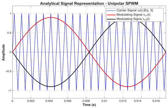
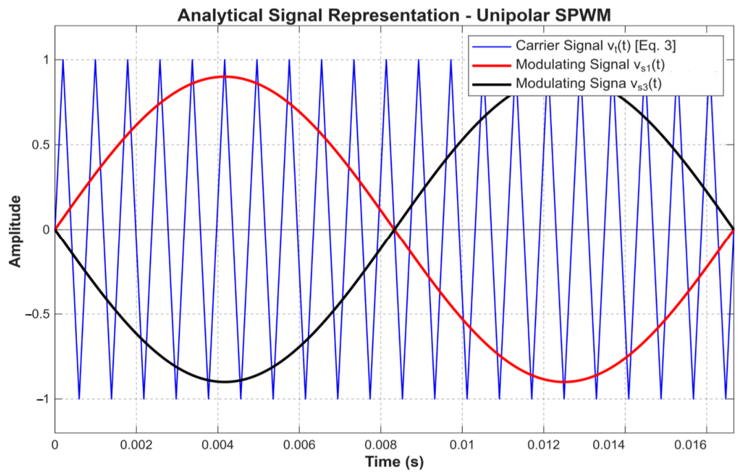
For the unipolar technique, two identical sinusoidal modulating signals are generated in frequency and amplitude (Equations (12) and (13)), but phase-shifted by π radians (180°) relative to each other, along with a high-frequency carrier signal. This is illustrated in Figure 1.

v_s1(t) = A_ssin(2πf_gt)

(12)

v_s3(t) = A_ssin(2πf_gt + π) = −A_ssin(2πf_gt)

(13)

Figure 1. Analytical signal representation, unipolar SPWM.

The intersections between the modulating signals (Equations (12) and (13)) and the carrier define the error function e_x(t), whose zeros e_x(t) = 0 represent the crossing times t_cross,k

$$e_x(t)=A_s\sin \left(2\pi f_{g}t\right)-{\displaystyle \frac{2A_t}{\pi }}\arcsin \left(\sin \left(2\pi f_{c}t\right)\right)$$

(14)

$$e_x(t)=A_s\sin \left(2\pi f_{g}t+\pi \right)-{\displaystyle \frac{2A_t}{\pi }}\arcsin \left(\sin \left(2\pi f_{c}t\right)\right)$$

(15)

The derivative of the triangular signal (Equation (11) can be defined by parts, as shown in Equation (16):

$${\displaystyle \frac{d{v}_t(t)}{\mathit{dt}}}=4f_c\mathrm{sgn}\left(\cos \left(2\pi f_{c}t\right)\right)\hspace{1em}\mathrm{for} t\ne {\displaystyle \frac{2k+1}{4f_c}},\hspace{0.33em}k\in \mathbb{Z}$$

(16)

Consequently, the time derivative of the error function e_x(t) takes the form given in Equation (17).

$${\displaystyle \frac{d{e}_x(t)}{\mathit{dt}}}=2\pi f_g{A}_s\cos \left(2\pi f_{o}t+{\varphi }_x\right)-4f_c{A}_t\mathrm{sgn}\left(\cos \left(2\pi f_{c}t\right)\right)\hspace{1em}\mathrm{for} t\ne {\displaystyle \frac{2k+1}{4f_c}}$$

(17)

Equations (16) and (17) impose a fundamental restriction on the maximum and minimum peaks of the triangular signal, given by the set of points shown in Equation (16).

$$t_k={\displaystyle \frac{2k+1}{4f_c}}=\left\{{\displaystyle \frac{1}{4f_c}},{\displaystyle \frac{3}{4f_c}},{\displaystyle \frac{5}{4f_c}},\dots \right\},\hspace{1em}k\in \mathbb{Z}$$

(18)

It holds that cos(2πf_ct_k) = 0 and sin(2πf_ct_k) = ±1. At these vertices, the function v_t(t) has points where it is not differentiable, causing the denominator in the derivative to vanish $\sqrt{1-{(\pm 1)}^2}=0$ and ${\displaystyle \frac{d{v}_t}{\mathit{dt}}}$ to exhibit finite-jump discontinuities.

This property of non-differentiability prevents or severely impairs the convergence of derivative-based root-finding methods, such as the Newton–Raphson method or the secant method, which may diverge or become trapped in infinite loops if the evaluation interval includes a vertex t_k.

On the other hand, the function v_t(t) defined in Equation (3) is strictly continuous throughout the real domain (v_t ∈ C⁰). Since Bolzano’s Theorem requires only the continuity of the integrand on a closed interval [t_a,t_b] and not the existence of its derivative (C¹), this is quantitatively guaranteed by Equation (17).

e_x(t_a) ⋅ e_x(t_b) ≤ 0

(19)

There exists at least one real root t^* ∈ [t_a,t_b] such that e_x(t^*) = 0. This theoretical soundness justifies the choice of the Bolzano-based offline algorithm, guaranteeing the convergence and numerical stability of the switching times even at the vertices of the carrier.

The theoretical switching instants correspond to the roots of the differential error functions e₁(t) and e₃(t), associated with the branches of the inverter; this is shown in Equations (20) and (21).

e₁(t) = v_s1(t) − v_t(t) = 0

(20)

e₃(t) = v_s3(t) − v_t(t) = 0

(21)

Since the algorithm operates in a discrete environment sampled at a certain period, $T_s={\displaystyle \frac{1}{\mu f_c}}$.

• where μ represents the oversampling factor per carrier period; the determination of the firing angles is performed computationally by applying the sign-change criterion derived from Bolzano’s Theorem for the intermediate value. See Equation (22).

e_x(t_k)e_x(t_k+1) ≤ 0

(22)

where x ∈ {1,3} indicates the branch being evaluated and t_k represents the k-th time sampling point. When the inequality holds (22), the crossing time is calculated t_cross,k≈t_k and is projected onto the fundamental angular domain β_k by means of the linear transformation shown in Equation (23).

β_k = 2πf_gt_cross,k [rad] ≡ 360°f_gt_cross,k [degrees]

(23)

where t_cross,k is not the exact intersection but rather the nearest discrete time point; however, if the oversampling factor μ is 1000 times higher than the carrier frequency, the error in the intersections is minimal.

Within each period of the fundamental signal, $T_g={\displaystyle \frac{1}{f_g}}$. The algorithm detects exactly 2m_f switching angles per branch, generating the trigger event vector $\beta ={[{\beta }_1,{\beta }_2,\dots ,{\beta }_{2m_f}]}^T$.

2.2. Switching Logic and Output Voltage

Event-based temporal reconstruction transforms the angle vectors into logic gate signals G_j(t) ∈ {0,1} of semiconductors. Unipolar SPWM modulation requires that the switches in the same branch operate in a complementary manner to prevent a short circuit with the DC bus. The switching logic is shown in Equations (24)–(26).

$$G_1(t)=\left\{\begin{array}{ll}1,\hfill & \mathrm{if} v_{s1}(t)\ge v_t(t)\hfill \\ 0,\hfill & \mathrm{if} v_{s1}(t)<v_t(t)\hfill \end{array}\right.$$

(24)

$$G_3(t)=\left\{\begin{array}{ll}1,\hfill & \mathrm{if} v_{s3}(t)\ge v_t(t)\hfill \\ 0,\hfill & \mathrm{if} v_{s3}(t)<v_t(t)\hfill \end{array}\right.$$

(25)

G₂(t) = 1 − G₁(t),  G₄(t) = 1 − G₃(t)

(26)

The inverter’s differential output voltage, (V_out(t)), is defined as the potential difference between the intermediate nodes of both legs. In the absence of voltage drops across the semiconductor devices and assuming a DC bus voltage (V_dc), the analytical expression for the instantaneous output voltage is given by Equation (27):

V_out(t) = V_dc[G₁(t) − G₃(t)]

(27)

Unlike bipolar switching, the algebraic balance of the Boolean signals in Equation (27) allows for V_out(t), assuming three discrete voltage states, +V_dc, 0 and −V_dc, doubling the effective switching frequency seen by the output filter to 2f_c and significantly reducing current ripple [6,7].

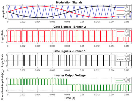
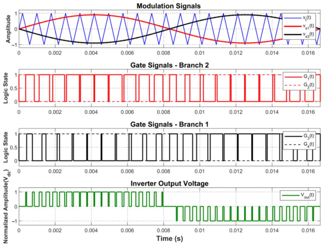
Figure 2 shows unipolar SPWM modulation with a modulation index of 0.9, a fundamental frequency of 60 Hz, a V_dc normalized to 1, m_f of 21, a carrier frequency 21 times greater than the fundamental frequency, and μ = 1000.

Figure 2. SPWM modulation in an inverter.

The figure above shows the sinusoidal signals that are 180° out of phase and the high-frequency carrier signal. The two middle figures (red and black signals) show the gate signals for G₁(t) and G₃(t), as well as their complements, G₂(t) and G₄(t). Finally, the bottom figure (green signal) shows the output voltage of a full-bridge inverter with SPWM modulation.

2.3. LCL Filter Design, DC Bus, Phase Compensation and Link Capacitance

The inverter design requires sizing the passive filter components to meet power quality criteria and maintain the stability of the DC bus. Based on Average Active Power (P_avg) and Grid Peak Voltage (V_g), the fundamental Peak Current Injected into the Grid (I_g) for a unity power factor is defined by Equation (28).

$$I_g={\displaystyle \frac{2P_{\mathit{avg}}}{V_g}}$$

(28)

The system is configured based on the operating frequencies, the fundamental angular frequency of the grid, ω_g = 2πf_g and the dominant harmonic angular frequency, ω_n = 2πf_n, which is closely related to the switching frequency of the SPWM technique [6,7].

For the design of the LCL filter, the dimensionless design factors α and β are introduced, which relate the desired attenuation to the ratio of the inductance on the inverter side to that on the grid side [6]. This is shown in Equations (29) and (30).

α = ω_n²L₁C_f

(29)

$$\beta ={\displaystyle \frac{L_1}{L_2}}$$

(30)

The LCL filter is essential for attenuating the high-frequency harmonics generated by transistor switching; it is calculated based on the current ripple on the inverter side (%r_inv), the average power injected into the grid, the proposed values of α and β, and the grid voltage. The design equations for the LCL filter are shown in Equations (23)–(25).

$$L_1={\displaystyle \frac{100V_g{V}_{\mathit{in}}\left(\alpha -\beta \right)}{{\omega }_n\%r_{\mathit{inv}}{P}_{\mathit{avg}}\left(-\beta +\alpha -1\right)}}$$

(31)

$$L_2={\displaystyle \frac{L_1}{\beta }}$$

(32)

$$C_f={\displaystyle \frac{\%r_{\mathit{inv}}{P}_{\mathit{avg}}\alpha \left(-\beta +\alpha -1\right)}{{100}_{\mathit{Vg}}{V}_{\mathit{in}}{\omega }_n\left(\alpha -\beta \right)}}$$

(33)

where V_in is the voltage of the predominant harmonic derived from the triangular carrier frequency.

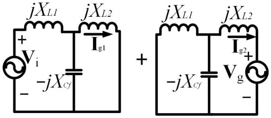
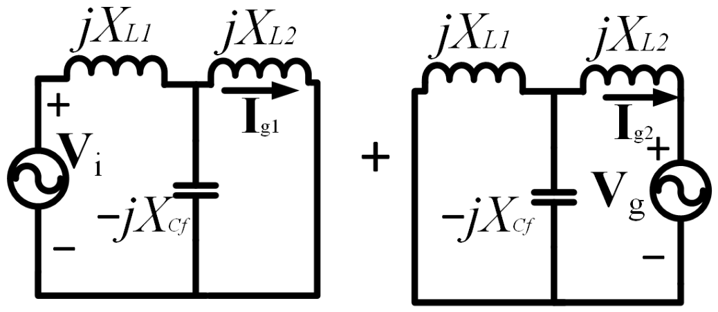
The LCL filter connected to the inverter and the grid can be represented by two equivalent circuits (See Figure 3) using the superposition theorem. The sum of the individual responses of each circuit will be the total response of the LCL filter.

Figure 3. LCL filter divided by superposition theorem.

In the figure, $\left(X_{L_1}\hspace{0.17em}{X}_{L_2}\hspace{0.17em}{X}_{C_f}\right)$ are the reactance of each filter element, V_i is the phasor at the fundamental harmonic (60 Hz) of the inverter’s unipolar SPWM modulation, V_g is the phasor of the grid voltage, and $\left(I_{{\mathrm{g}}_1}\hspace{0.17em}{I}_{{\mathrm{g}}_2}\right)$ are the grid current in each circuit equivalent.

Solving the circuit shown in the figure for $I_{{\mathrm{g}}_1}$ and $I_{{\mathrm{g}}_2}$ yields the expressions shown in Equations (34) and (35):

$$I_{g_1}={\displaystyle \frac{V_{{\mathrm{C}}_{\mathrm{f}}}}{Z_{L_2}}}=-{\displaystyle \frac{V_i\angle {\varphi }_{\mathit{spwm}}j{X}_{C_f}}{X_{C_f}{X}_{L_1}+X_{C_f}{X}_{L_2}-X_{L_1}{X}_{L_2}}}$$

(34)

where $V_{{\mathrm{C}}_{\mathrm{f}}}$ is the voltage phasor of capacitor C_f and $Z_{L_2}$ is the impedance of inductor L₂.

$${{\rm I}}_{{\mathrm{g}}_2}={\displaystyle \frac{V_{\mathrm{g}}}{Z_{L_2}+Z_{\mathit{eq}2}}}=-{\displaystyle \frac{V_g\angle 0°\left(X_{C_f}-X_{L_1}\right)j}{X_{C_f}{X}_{L_1}+X_{C_f}{X}_{L_2}-X_{L_1}{X}_{L_2}}}$$

(35)

where Z_eq2 is the equivalent impedance of the parallel circuit consisting of L₁ and C_f. Adding (34) and (35), Equation (36) is obtained, which is the total current injected into the grid at the fundamental harmonic.

$$I_{\mathrm{g}}=-{\displaystyle \frac{V_g\angle 0°j\left(X_{C_f}-X_{L_1}\right)-V_i\angle {\varphi }_{\mathit{spwm}}\left(j{X}_{C_f}\right)}{X_{C_f}{X}_{L_1}+X_{C_f}{X}_{L_2}-X_{L_1}{X}_{L_2}}}$$

(36)

Solving for the V_i of Equation (36) for a power unit factor is shown in Equation (42).

$$V_i\angle {\varphi }_{\mathit{spwm}}={\displaystyle \frac{V_g\left(j{X}_{C_f}-j{X}_{L_1}\right)-I_g\left(X_{C_f}{X}_{L_1}+X_{C_f}{X}_{L_2}-X_{L_1}{X}_{L_2}\right)}{\left(j{X}_{C_f}\right)}}$$

(37)

Substituting the value of each reactance of the LCL filter elements yields Equation (38).

$$V_i=\sqrt{{\left(V_g-{\omega }^2{L}_1{C}_f{V}_g\right)}^2+{\left(\omega L_1{I}_g+\omega L_2{I}_g-{\omega }^3{L}_1{L}_2{C}_f{I}_g\right)}^2}$$

(38)

The DC bus voltage V_dc cannot be arbitrary; it must be greater than V_g to prevent energy from flowing back from the grid to the inverter and high enough to prevent overmodulation (ensuring linear control via the modulation index m).

The modulation index relates the DC bus voltage V_dc and the input voltage V_i of the fundamental harmonic in the LCL filterThis is shown in Equation (39).

V_i = mV_dc

(39)

Substituting Equation (38) into Equation (39) and solving for V_dc yields Equation (40):

$$V_{\mathit{dc}}={\displaystyle \frac{V_i}{m}}={\displaystyle \frac{\sqrt{{\left(V_g-{{\omega }_g}^2{L}_1{C}_f{V}_g\right)}^2+{\left({\omega }_g{L}_1{I}_g+\omega L_2{I}_g-{{\omega }_g}^3{L}_1{L}_2{C}_f{I}_g\right)}^2}}{m}}$$

(40)

The injection of current into the power grid requires that the voltage generated by the inverter (modulated by SPWM) be ahead by a specific angle relative to the grid voltage. This angle compensates for the phase shift and voltage drop caused by the reactive components of the LCL filter at the fundamental frequency [6]. This angle is shown in Equation (41).

$${\varphi }_{\mathit{spwm}}=\arctan \left({\displaystyle \frac{{\omega }_g{I}_g\left(L_1+L_2-{\omega }_g^2{L}_1{L}_2{C}_f\right)}{V_g\left(1-{\omega }_g^2{L}_1{C}_f\right)}}\right)$$

(41)

This angular value is fed back to the angle obtained from the measurement of the grid phase via the PLL. This feedback ensures that the carrier’s zero crossings are correctly aligned, guaranteeing the synchronized injection of active power.

Finally, to absorb the instantaneous power fluctuations inherent in a single-phase system and keep the voltage ripple of the DC bus within a regulatory tolerance limit, the DC bus (DC-link) capacitor is sized by incorporating the angle effect from Equation (41). The DC bus capacitor is calculated using Equation (42).

$$C_{\mathit{link}}={\displaystyle \frac{P_{\mathit{avg}}\left(2-\cos \left({\varphi }_{\mathit{spwm}}\right)\right)}{V_g{\omega }_g\Delta V_{\mathit{dc}}}}$$

(42)

2.4. Real-Time Synchronization with the Grid

While the switching angles are generated in a calculated manner, feeding power into the grid requires strict real-time synchronization. To achieve this, the algorithm implemented in the dynamic simulation extracts the instantaneous phase of the grid using a PLL loop.

The phase variable estimated by the PLL, denoted as ω_g(t), is bounded within the interval [0, 2π]. To relate this phase to the precalculated crossing times t_cross, an affine transformation is applied that projects the angular domain onto the time domain of the local cycle, incorporating the phase angle ϕ_spwm obtained in Equation (41) for active power control. This operation is shown in Equation (43).

$$t_{\mathit{cycle}}\left(t\right)={\displaystyle \frac{{\omega }_g\left(t\right)+{\varphi }_{\mathit{spwm}}}{2\pi f_g}}$$

(43)

where t_cycle(t) represents the elapsed time within the period of the fundamental grid frequency, bounded by $\left[0,\hspace{0.17em}{\displaystyle \frac{1}{f_g}}\right]$.

The trigger controller operates as a finite-state machine that requires historical memory to maintain the consistency of the gate signals. In a discrete simulation environment, where k represents the current sampling time and k − 1 the previous one, the algorithm detects the zero-crossing of the phase (the start of a new cycle) by evaluating the discrete derivative of the local time. This is shown in Equation (44).

Δt_cycle[k] = t_cycle[k] − t_cycle[k − 1]

(44)

When Δt_ciclo[k] < 0, the system identifies the transition from 2π to 0 radians. At this singular event, the pointers of the intersection vectors $\left(p_{t{r}_1}\hspace{0.17em}{p}_{t{r}_2}\right)$ are reset to their initial values. It is imperative to note that the logic states of the gates $\left(e_{s{t}_1}\hspace{0.17em}{e}_{s{t}_3}\right)$ are not forced to zero during this transition, ensuring the continuity of the waveform and preventing spurious transients (glitches) in the inverter.

Pulse generation is governed by a sequential evaluation function (See Equation (45)). For a branch x ∈ {1,3}, the logic state of the main gate E_x is toggled if, and only if, the current cycle time exceeds the programmed crossing time, and the pointer has not exceeded the size of the precalculated crossing vector N_x.

$$E_x[k]=\left\{\begin{array}{ll}1-E_x[k-1],\hfill & \mathrm{if} t_{\mathit{cycle}}[k]\ge t_{\mathit{cross},x}[p_{t{r}_x}] \mathrm{y} p_{t{r}_x}\le N_x\hfill \\ E_x[k-1],\hfill & \mathrm{in} \mathrm{any} \mathrm{other} \mathrm{case}\hfill \end{array}\right.$$

(45)

Immediately after a valid state transition, the read index is incremented by one $(p_{t{r}_x}\leftarrow p_{t{r}_x}+1)$, preparing the system for the next switching event.

Finally, the topology of the full-bridge inverter requires that the semiconductor devices in the same leg do not conduct simultaneously. Based on the main states evaluated in Equation (34), the complementary trigger signals for branches (G₁ G₂) and (G₃ G₄) are mathematically derived as shown in Equations (46) and (47).

G₁(t) = E₁(t),  G₂(t) = 1 − E₁(t)

(46)

G₃(t) = E₃(t),  G₄(t) = 1 − E₃(t)

(47)

This ideal complementarity, defined in Equations (35) and (36), assumes perfect switches. In the physical hardware implementation (using MOSFETs or IGBTs), this block must be cascaded with a dead-time generator to compensate for the intrinsic turn-on and turn-off delays of the transistors.

2.5. Algorithm for Switching Time Calculation in a Unipolar SPWM Grid-Connected Full-Bridge Inverter

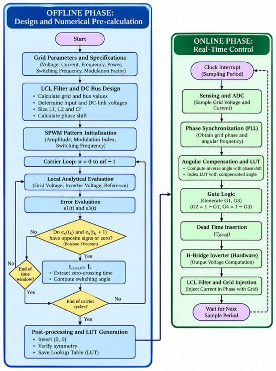
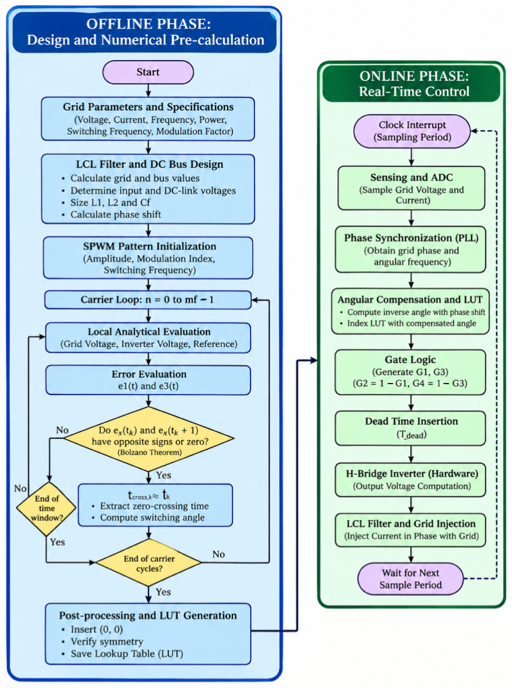
The algorithm described in this paper can be represented by a flowchart (Figure 4). This flowchart describes how the switching signal generation strategy works for a full-bridge inverter connected to the grid, divided into two main stages: the “offline” phase, which corresponds to the design and preliminary numerical calculations, and the “online” phase, which is associated with the execution of real-time control.

Figure 4. Algorithm for switching time calculation in a unipolar SPWM grid-connected full-bridge inverter.

In the offline phase, the algorithm begins by defining the system’s electrical and operating parameters, including line voltage and current, fundamental frequency, average power, switching frequency, and modulation index. Based on these specifications, the LCL filter and the DC bus are sized.

Next, the parameters required to generate the SPWM pattern are initialized. The algorithm then enters a loop synchronized with the carrier signal periods. For each interval, an analytical evaluation of the relevant signals is performed, considering the reference signal, the inverter signal, and the grid signal. These signals are used to calculate the errors corresponding to each branch of the H-bridge.

The algorithm identifies the approximate switching instant by detecting sign changes in the errors. The process is repeated until the time window corresponding to each cycle of the carrier signal is completed, and then until all required cycles have been processed. Once the calculation is complete, the results undergo a post-processing stage in which the initial point is incorporated, and a Lookup Table (LUT) is generated. This table contains the switching angles or times that will subsequently be used by the real-time control system.

In the online phase, the algorithm begins operating when the control clock triggers a periodic interrupt. During each sampling period, the electrical variables of the grid—primarily voltage and current—are acquired. The measured signals are processed by a PLL, whose function is to determine the instantaneous phase and angular frequency of the grid. This information allows the inverter to remain synchronized with the electrical grid.

Next, the angle obtained by the PLL is compensated using the phase shift previously calculated during the offline phase. The compensated angle is used to perform the corresponding lookup in the LUT and obtain the required switching states for the inverter’s MOSFETs or IGBTs.

3. Results

This section will present the theoretical results (Offline Algorithm) and simulation results (Online Algorithm) for interconnection to the electrical grid.

3.1. Theoretical Results (Offline Algorithm: Example 1)

To evaluate the algorithm offline and generate the switching times and angles, the input parameters listed in Table 1 were used as the first example.

Table 1. Input parameters for the numerical analysis of SPWM modulation (Example 1).

Parameter	Symbol	Value
Carrier Signal Amplitude	At	1 V
Modulating Signal Amplitude	As	0.9 V
Carrier Signal Frequency	fc	600 Hz
Grid Frequency	fg	60 Hz
Modulation Index	m	0.9
Carrier Signal Period	Tc	0.0017 S
Frequency Modulation Index	mf	10
Oversampling Factor	μ	1000

The evaluation of the offline algorithm is based on the analytical intersection between the triangulated carrier v_t(t) and the phase-shifted sinusoidal modulating signals 180° with each other, $v_{s_1}(t)$ and $v_{s_3}(t)$. When processing signals in the discrete domain at a resolution given by μ = 1000 samples per carrier period f_s = μ ⋅ f_c = 0.6 MHz, applying Bolzano’s Theorem allows us to identify with high precision the sign changes in the error functions $e_1(t)=v_{s_1}(t)-v_t(t)$ and $e_3(t)=v_{s_3}(t)-v_t(t)$.

As a result of this sweep, an ordered sequence of crossing times t_cross,k is generated for each branch of the inverter. By transforming these instants into the fundamental angular domain using β_k = 360° ⋅ f_gt_cross,k, the switching vectors are synthesized and stored in the LUT (See Table 2), for the parameters specified in Table 1.

Table 2. Switching times and angles (Example 1).

Parameter	Sample
	1	2	3	4	5	6	7	8	9	10	11	12	13	14	15	16	17	18	19	20
$\begin{array}{l}{\beta }_{g_1}\\ \left(\mathrm{degrees}\right)\end{array}$	0°	15.78°	41.33°	47.96°	79.96°	81.94°	115.31°	118.88°	148.25°	159.09°	180°	200.86°	211.71°	241.08°	244.64°	278.01°	280°	312°	318.63°	344.18
$\begin{array}{l}{\beta }_{g_3}\\ \left(\mathrm{degrees}\right)\end{array}$	0°	20.86°	31.71°	61.08°	64.64°	98.01	100	132	138.63	164.18°	180°	195.78°	221.33°	227.96°	259.96°	261.94°	295.31°	298.88°	328.25°	339.09°
$\begin{array}{l}{t}_{\mathit{cross},1}\\ (\mathit{mS})\end{array}$	0	0.73	1.9	2.2	3.7	3.8	5.3	5.5	6.9	7.4	8.3	9.3	9.8	11.2	11.3	12.9	13	14.4	14.8	15.9
$\begin{array}{l}{t}_{\mathit{cross},3}\\ (\mathit{mS})\end{array}$	0	1	1.5	2.8	3	4.5	4.6	6.1	6.4	7.6	8.3	9.1	10.2	10.6	12	12.1	13.7	13.8	15.2	15.7

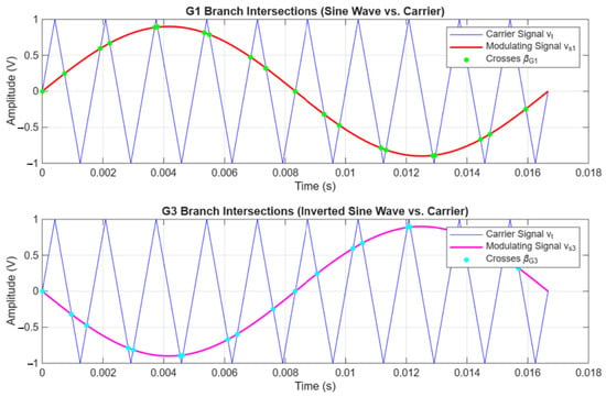
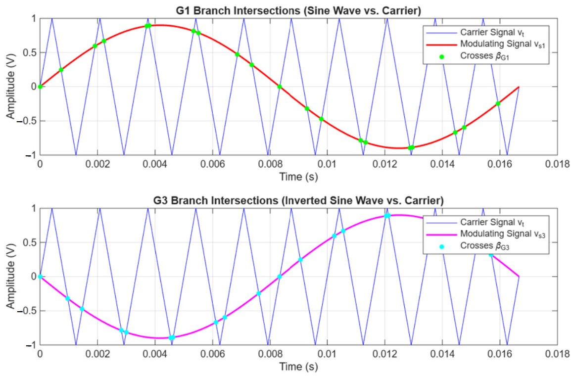
Figure 5 shows the distribution of the crossings over the fundamental period $T_g={\displaystyle \frac{1}{f_g}}$.

Figure 5. Intersections between the triangular carrier signal and the modulating signals (Example 1).

The red signal represents the positive sine wave modulator; the blue signal represents the 600 Hz triangular carrier; the green dots represent the intersections between these signals with a modulation index of 0.9. The purple signal represents the negative sine wave modulator; the light blue dots represent the intersections between these signals.

3.2. Theoretical Results (Offline Algorithm: Example 2)

To evaluate the algorithm offline and generate the switching times and angles, the input parameters shown in Table 3 were used as a second example.

Table 3. Input parameters for the numerical analysis of SPWM modulation (Example 2).

Parameter	Symbol	Value
Carrier Signal Amplitude	At	1 V
Modulating Signal Amplitude	As	0.9 V
Carrier Signal Frequency	fc	10.02 KHz
Grid Frequency	fg	60 Hz
Modulation Index	m	0.9
Carrier Signal Period	Tc	99.8 µS
Frequency Modulation Index	mf	167
Oversampling Factor	μ	1000

The second evaluation of the offline algorithm follows the same principle as Example 1, based on the analytical intersection between the triangulated carrier v_t(t) and the sinusoidal modulating signals that are phase-shifted $v_{s_1}(t)$ and $v_{s_3}(t)$ relative to one another. When processing the signals in the discrete domain with a resolution given by samples μ = 1000 per period of the carrier f_s = μ ⋅ f_c = 10.02 MHz, the application of Bolzano’s theorem allows us to identify the sign changes in the error functions with high precision $e_1(t)=v_{s_1}(t)-v_t(t)$ and $e_3(t)=v_{s_3}(t)-v_t(t)$.

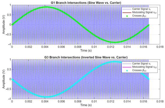
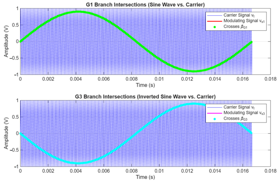
As a result of this sweep, an ordered sequence of crossing times is generated for each branch of the inverter (t_cross1 and t_cross3), as well as the switching angles (${\beta }_{g_1}$ and ${\beta }_{g_3}$). For this example, the table of angles and times is not shown, since it is a LUT with 334 values for each parameter. However, Figure 6 shows the intersections of the modulating signals with the carrier for Example 2.

Figure 6. Intersections between the triangular carrier signal and the modulating signals (Example 2).

The blue signal represents the 10.02 kHz triangular carrier; the green dots represent the intersections between the positive sine wave and the carrier at a modulation index of 0.9; the light blue dots represent the intersections between the carrier signal and the negative sine wave.

Once the intersection events have been identified, the algorithm determines the switching logic states for the four MOSFETs or IGBTs in the inverter G₁ and G₄. According to the direct comparison logic:

The upper switch G₁(t) assumes a high state (1) when v_s1(t) ≥ v_t(t) and a low state (0) otherwise. The lower switch G₂(t) operates in a strictly complementary manner G₂ = 1 − G₁. The upper switch G₃(t) is activated when v_s3(t) ≥ v_t(t) while G₄(t) acts as its complement G₄ = 1 − G₃.

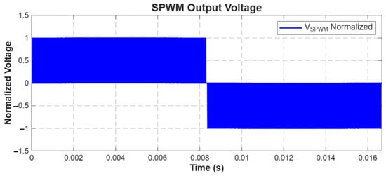
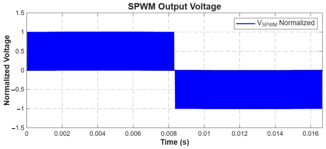
The differential voltage generated between the central nodes of both branches of the inverter is obtained through a linear combination of the logic states (See Equation (27)). This waveform is shown in Figure 7.

Figure 7. SPWM output voltage (Example 2).

The theoretical results demonstrate the synthesis of a three-level voltage waveform: [+V_dc 0 − V_dc]. During the negative half-cycle of the reference 0 ≤ ω_gt < π, the output voltage switches solely between [ 0 + V_dc]. Similarly, during the positive half-cycle π ≤ ω_gt < 2π, the output switches between [−V_dc 0 ].

This three-level feature doubles the effective frequency of the dominant harmonic in the output voltage relative to the switching frequency of the transistors 2f_c = 20.04 kHz, shifting the unwanted spectral content toward high-frequency bands. As a direct result, current ripple is reduced and the physical dimensions of the LCL filter’s inductors L₁ and L₂ are optimized [6].

3.3. Simulation Results (Online Algorithm)

To validate the performance of the switching pattern obtained using the offline algorithm and confirm the system’s ability to inject power into the power grid, a full dynamic model of the system was implemented in the MATLAB/Simulink (2024b) environment.

The real-time control architecture operates by continuously reading the grid voltage V_g(t). Based on this signal, the Phase Locked Loop (PLL) blocks estimate the fundamental angular position of the grid (ϕ_g(t)), in real time.

To compensate for the intrinsic phase shift introduced by the reactive elements of the LCL filter, the previously calculated phase correction ϕ_spwm (Equation (41)) is applied, yielding the inverter reference phase ϕ_inv(t) = ϕ_g(t) + ϕ_spwm. This compensated angle acts as an input pointer to index the LUT containing the switching angles β_k precalculated by the offline algorithm. The LUT outputs activate the gates G₁ to G₄, which control the MOSFETs/IGBTs of the Full-Bridge Inverter.

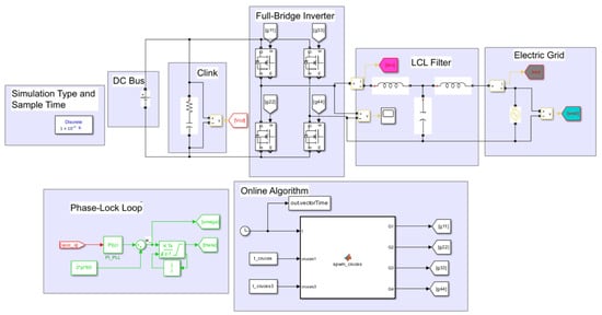
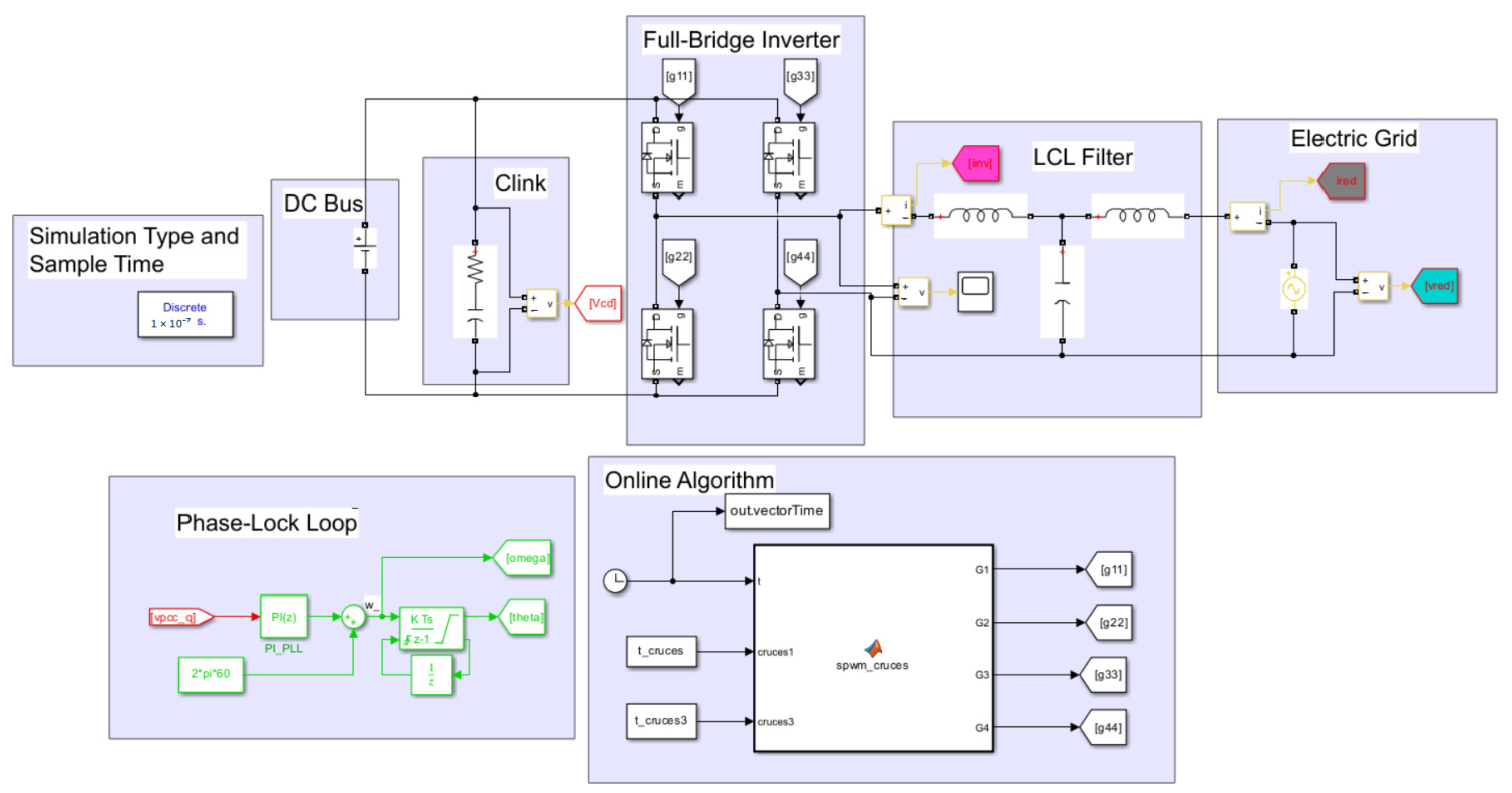
The diagram of the single-phase inverter connected to the power grid, implemented in Simulink, is shown in Figure 8.

Figure 8. Online-algorithm-controlled full-bridge inverter connected to the grid.

Figure 8 shows the block diagram of the system simulated, with its main stages outlined by the lilac-colored boxes. The simulation parameters in the discrete domain are specified in the upper-left corner, configured with a fixed integration step of 1 × 10⁷. The power stage, located in the upper center, consists of the DC bus source, the DC-link capacitor with its equivalent series resistance (ESR), and the full-bridge inverter composed of four MOSFETs. Connected to the output of the H-bridge is the LCL filter, which couples the system with the power grid for active power injection. The control stage, located in the lower section (from left to right), incorporates a discrete PLL to extract the phase of the grid voltage, followed by the MATLAB Function block that executes the online algorithm. This block takes as input the crossing times precalculated by the offline algorithm (stored in the workspace) and synthesizes the properly synchronized logic trigger signals to the semiconductor gates.

The input parameters for the simulated system are shown in Table 4.

Table 4. System input parameters.

Parameter	Symbol	Value
Peak voltage of the electrical grid	Vg	180 V
Alpha parameter (LCL filter design)	α	3.29
Beta Parameter (LCL filter design)	β	1
mnsw Parameter (for CD bus)	mnsw
Grid Frequency	fg	60 Hz
Modulation Index	m	0.9
Carrier Frequency	fc	10,020 Hz
Average Power	Pavg	4 kW
Percentage of Current Ripple in the Inverter	%rinv	10
Oversampling Factor	μ	1000

The following shows the calculated parameters (See Table 5) that are used in the simulation and the algorithms (online and offline).

Table 5. Parameters calculated for the simulation.

Parameter	Equation	Value
Frequency of the dominant harmonic	fn = 2fc − fg	19.98 kHz
Angular frequency of the dominant harmonic)	ωn = 2πfn	1.25 × 105 rad/s
Peak current injected into the grid	$I_g={\displaystyle \frac{2P_{\mathit{avg}}}{V_g}}$	44.4444 A
DC Bus Voltage	$V_{\mathit{dc}}=\sqrt{{\displaystyle \frac{A}{m^2-B}}}$	200.4432 V
LCL Filter Capacitor	$C_f={\displaystyle \frac{\%r_{\mathit{inv}}{P}_{\mathit{avg}}\alpha \left(-\beta +\alpha -1\right)}{{100}_{\mathit{Vg}}{V}_{\mathit{in}}{\omega }_n\left(\alpha -\beta \right)}}$	5.7957 × 10−7 F
LCL Filter Inductor 1	$L_1={\displaystyle \frac{100V_g{V}_{\mathit{in}}\left(\alpha -\beta \right)}{{\omega }_n\%r_{\mathit{inv}}{P}_{\mathit{avg}}\left(-\beta +\alpha -1\right)}}$	3.602 × 10−4 H
LCL Filter Inductor 2	$L_2={\displaystyle \frac{L_1}{\beta }}$	3.602 × 10−4 H
LCL Filter Phase Shift Angle	${\varphi }_{\mathit{spwm}}=\arctan \left({\displaystyle \frac{{\omega }_g{I}_g\left(L_1+L_2-{\omega }_g^2{L}_1{L}_2{C}_f\right)}{V_g\left(1-{\omega }_g^2{L}_1{C}_f\right)}}\right)$	0.067 rad or 3.83°
Link Capacitor	$C_{\mathit{link}}={\displaystyle \frac{P_{\mathit{avg}}\left(2-\cos \left({\varphi }_{\mathit{spwm}}\right)\right)}{V_g{\omega }_g\Delta V_{\mathit{dc}}}}$	0.002 F
Frequency Modulation Index	mf	167

The following section analyzes the waveforms obtained during the simulation of the inverter connected to the power grid. The evaluation focuses on the response of the online algorithm, synchronization via the discrete PLL, the currents in the LCL filter, and the transfer of active power to the grid.

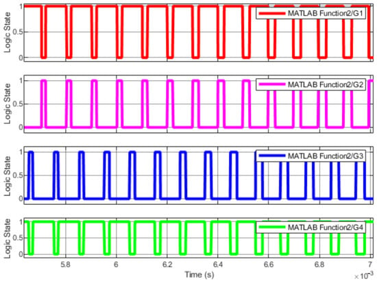
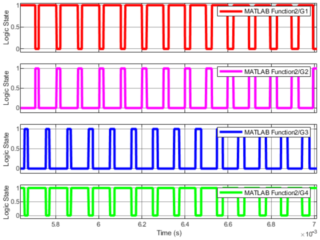
The switching response of the online block generates the four logic trigger signals G₁ G₂ G₃ G₄ based on the LUT synchronized with the phase of the grid. Figure 9 shows the complementary behavior between the transistors in each branch. The signals in Branch A G₁ G₂ and Branch B G₃ G₄ exhibit the phase shift characteristic of the unipolar SPWM technique, modulating the switching at the f_c.

Figure 9. Logic signals of the gates.

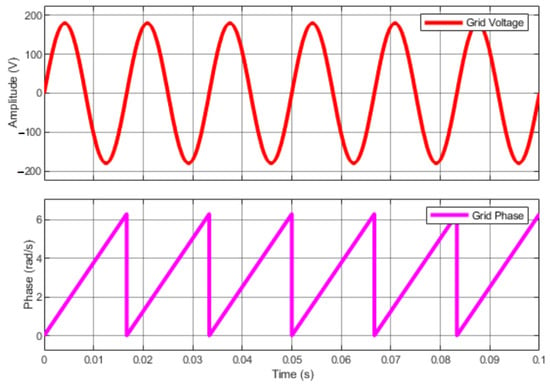
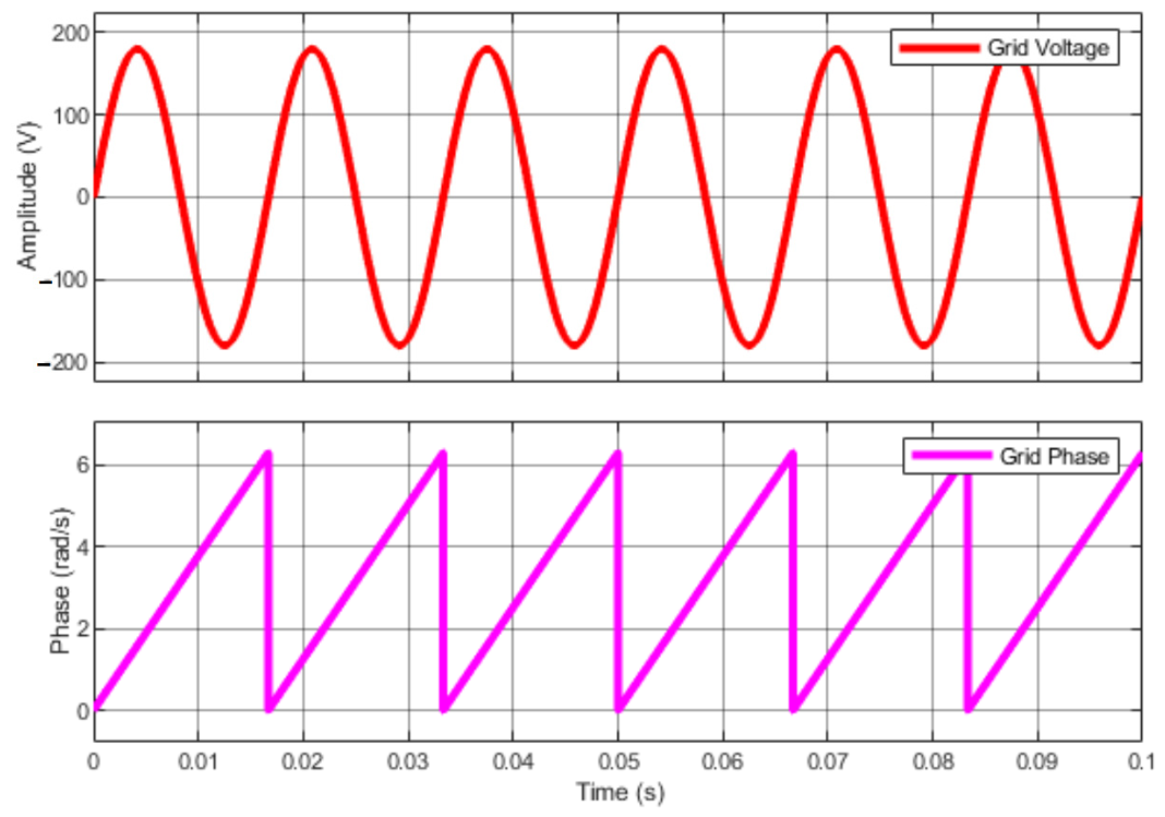
The tracking of the fundamental phase of the mains voltage is evaluated based on the response of the discrete PLL. The PLL output signal ϕ_g synthesizes a periodic angular ramp with a range of [0, 2π], perfectly aligned with the rising zero crossings of the voltage V_g(t). This is shown in Figure 10.

Figure 10. Extraction of the fundamental angular phase using a discrete PLL.

This estimation allows the compensated phase ϕ_inv = ϕ_g + ϕ_spwm to serve as a precise pointer for traversing the switching time LUT.

To verify the adaptability and dynamic performance of the proposed online algorithm under non-ideal power grid conditions, the system was subjected to a test scenario involving variations in the grid’s fundamental frequency f_g. Since synchronization and parameter extraction depend on the correct reading of the reference sinusoidal signal, this analysis allows for an evaluation of the stability of the estimates in the presence of disturbances in the power system.

The two main parameters dynamically adjusted in the power and modulation stages during these grid frequency sweep or disturbance tests were: the SPWM phase angle, and the DC bus level.

Table 6 shows the variations in these parameters at different grid frequencies.

Table 6. Grid frequency variation.

Frequency	Element	Value
60 Hz	Vdc	201.8091 V
	ϕspwm	0.1342 rad or 7.68°
55 Hz	Vdc	201.15168 V
	ϕspwm	0.1230 rad or 7.047°
50 Hz	Vdc	201.2511 V
	ϕspwm	0.1117 rad or 6.4°

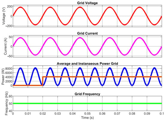
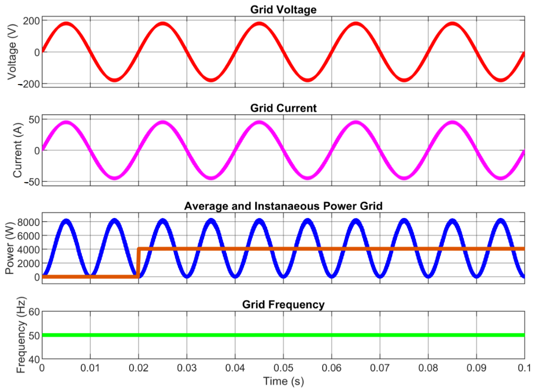
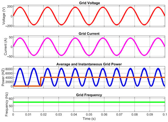
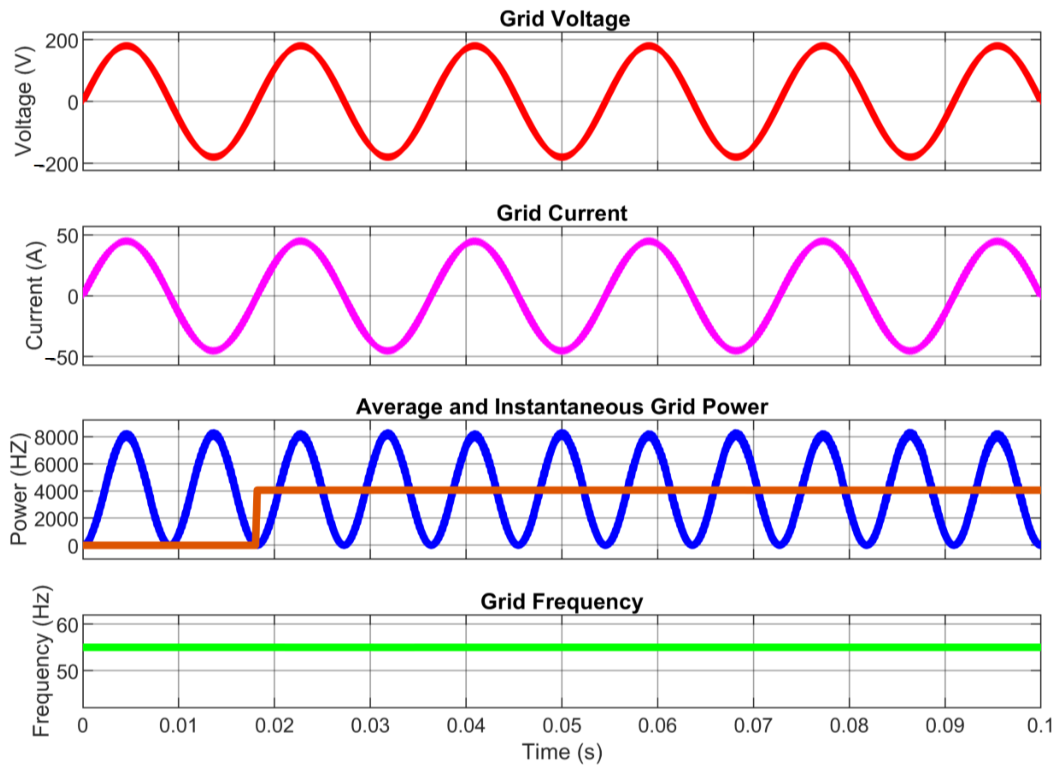
Figure 11 and Figure 12 graphically illustrate two examples of variations in the power grid frequency.

Figure 11. Test at a grid frequency of 50 Hz.

Figure 12. Test at a grid frequency of 55 Hz.

The red line represents the grid voltage, the pink line represents the current fed into the grid, the blue line represents the instantaneous power fed into the grid, and the same graph also shows the average power, which is calculated after one period 1/50 s has elapsed; finally, the green line represents the grid frequency.

The red line represents the grid voltage, the pink line represents the current fed into the grid, the blue line represents the instantaneous power fed into the grid, and the same graph also shows the average power, which is calculated after one period 1/55 s has elapsed; finally, the green line represents the grid frequency.

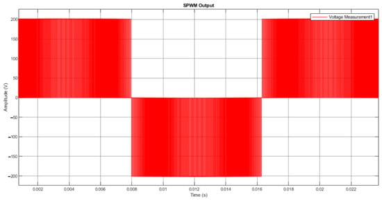
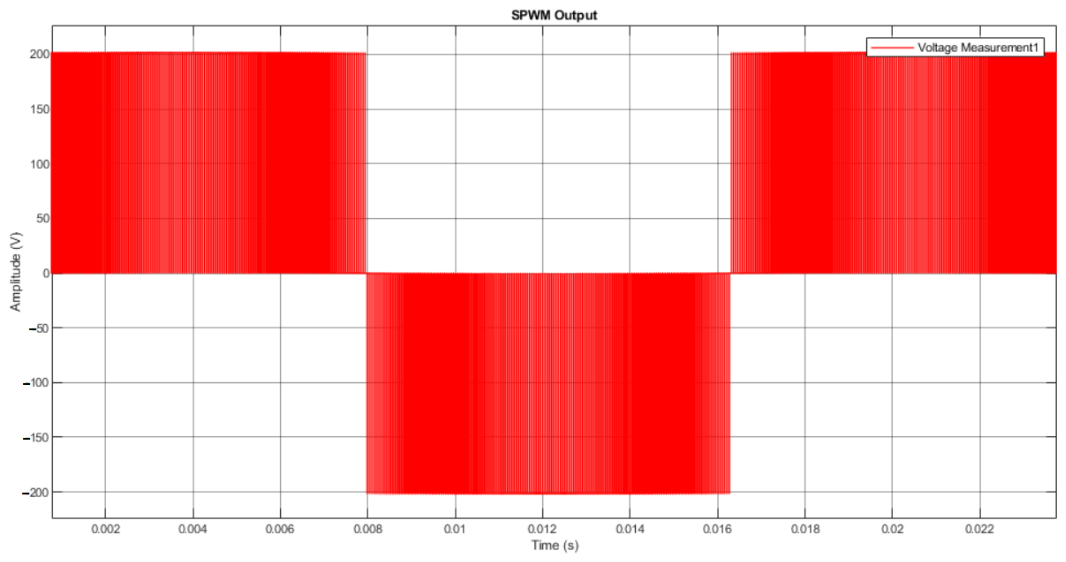
The output voltage at the inverter’s differential terminals, before entering the LCL filter (V_inv), exhibits a three-level modulated waveform [+V_dc 0 − V_dc] with V_dc = 200.4432 V. It switches between 0 V and +V_dc during the positive half-cycle, and between 0 and −V_dc during the negative half-cycle. This is shown in Figure 13.

Figure 13. Output voltage of unipolar SPWM modulation.

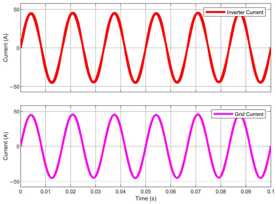
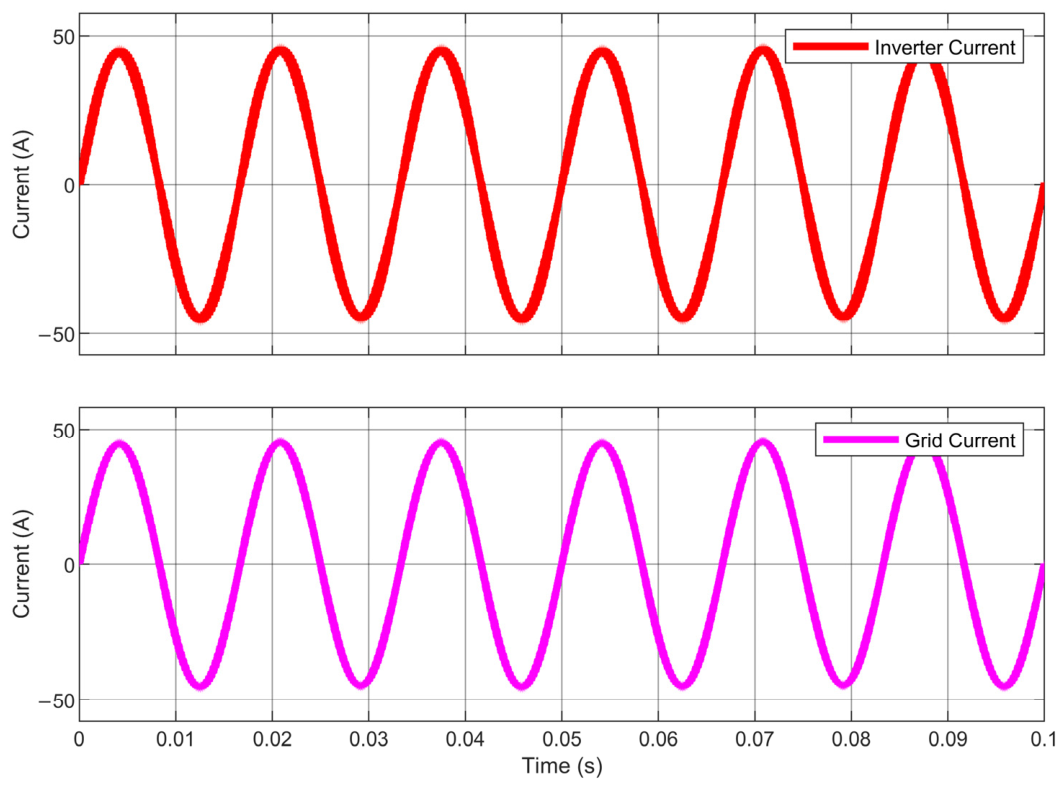
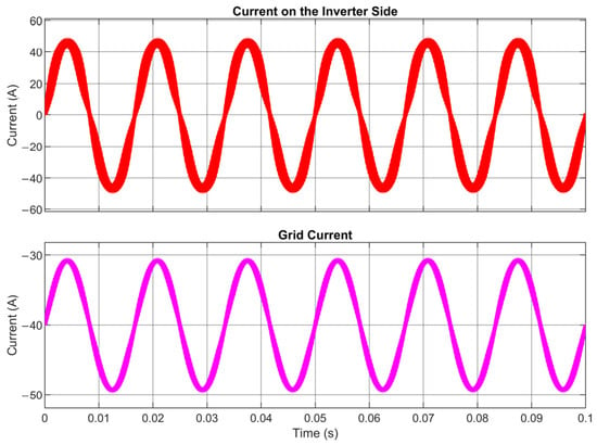
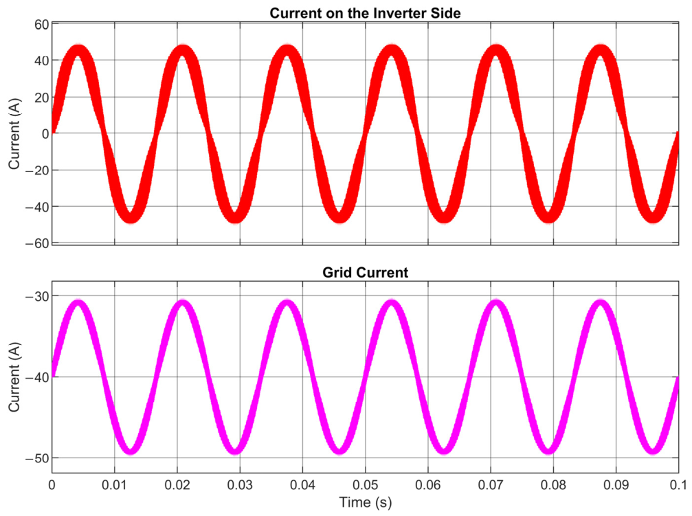
Regarding the results of the LCL filter simulation, the time response of the current in the inverter-side inductor (i_inv(t)) is compared to the grid-side current (i_g(t)). The current on the inverter side exhibits significant switching ripple centered around 2f_c − f_g, corresponding to the direct triggering of the MOSFETs. The current on the grid side exhibits a pure 60 Hz sinusoidal waveform. The implemented LCL filter effectively filters out high-frequency harmonic components, delivering clean current to the grid. This is shown in Figure 14.

Figure 14. Current on the inverter side and current injected into the grid.

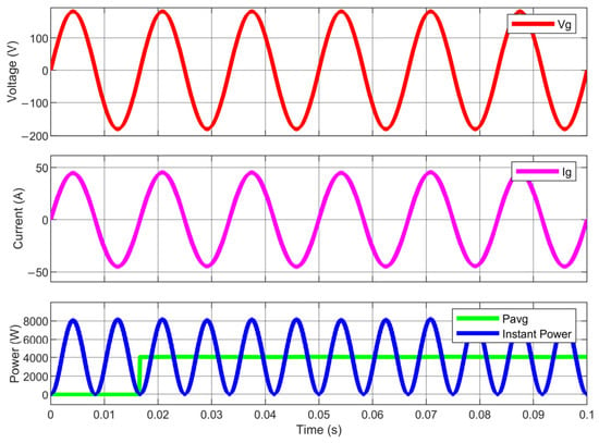
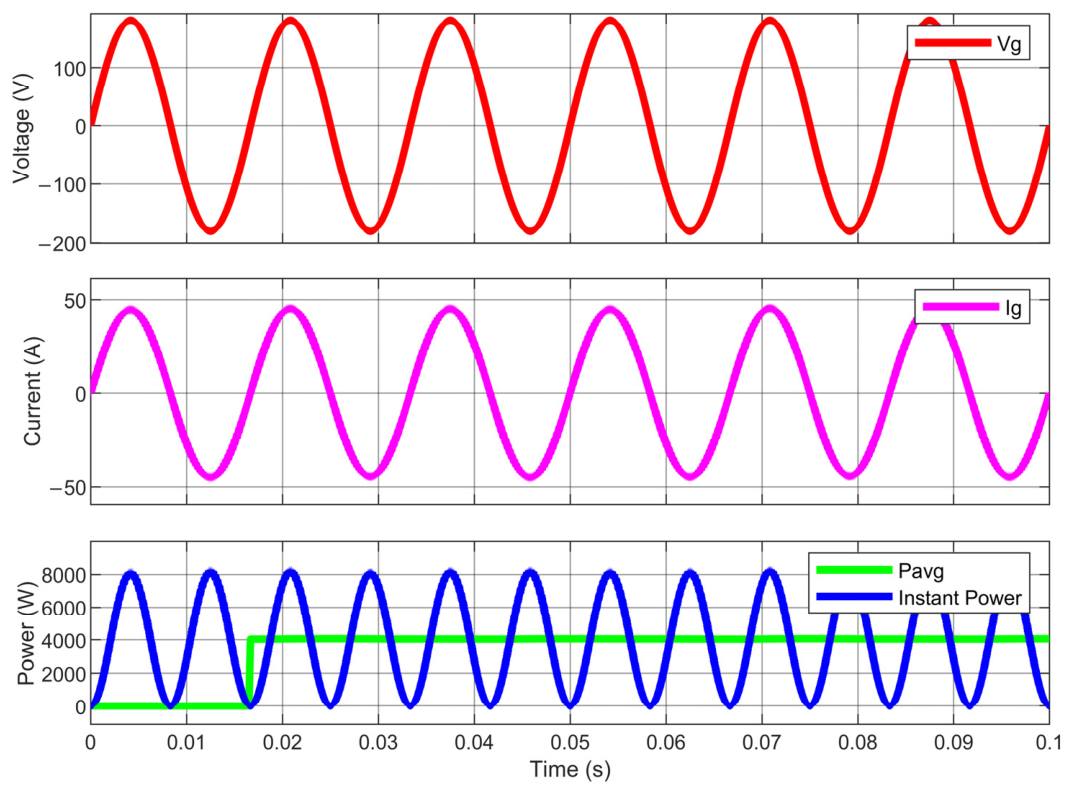
The overall performance of a grid-connected inverter is summarized by analyzing the phase relationship between the voltage (v_g(t)), the current (i_g(t)), and the instantaneous power transferred to the grid (p_g(t)). The injected current is perfectly in phase with the line voltage. This demonstrates that the phase compensation cancels out the phase shift introduced by the LCL filter, resulting in operation at a power factor of one. The average active power consistently reaches the nominal design value (P_avg = 4 kW) with negligible ripple in steady state. At the same time, the reactive power (Q(t)) remains bound at zero, confirming that the system does not exchange reactive power with the grid. All of this is shown in Figure 15.

Figure 15. Grid voltage, grid current, instantaneous power, and average power injected into the grid.

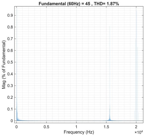
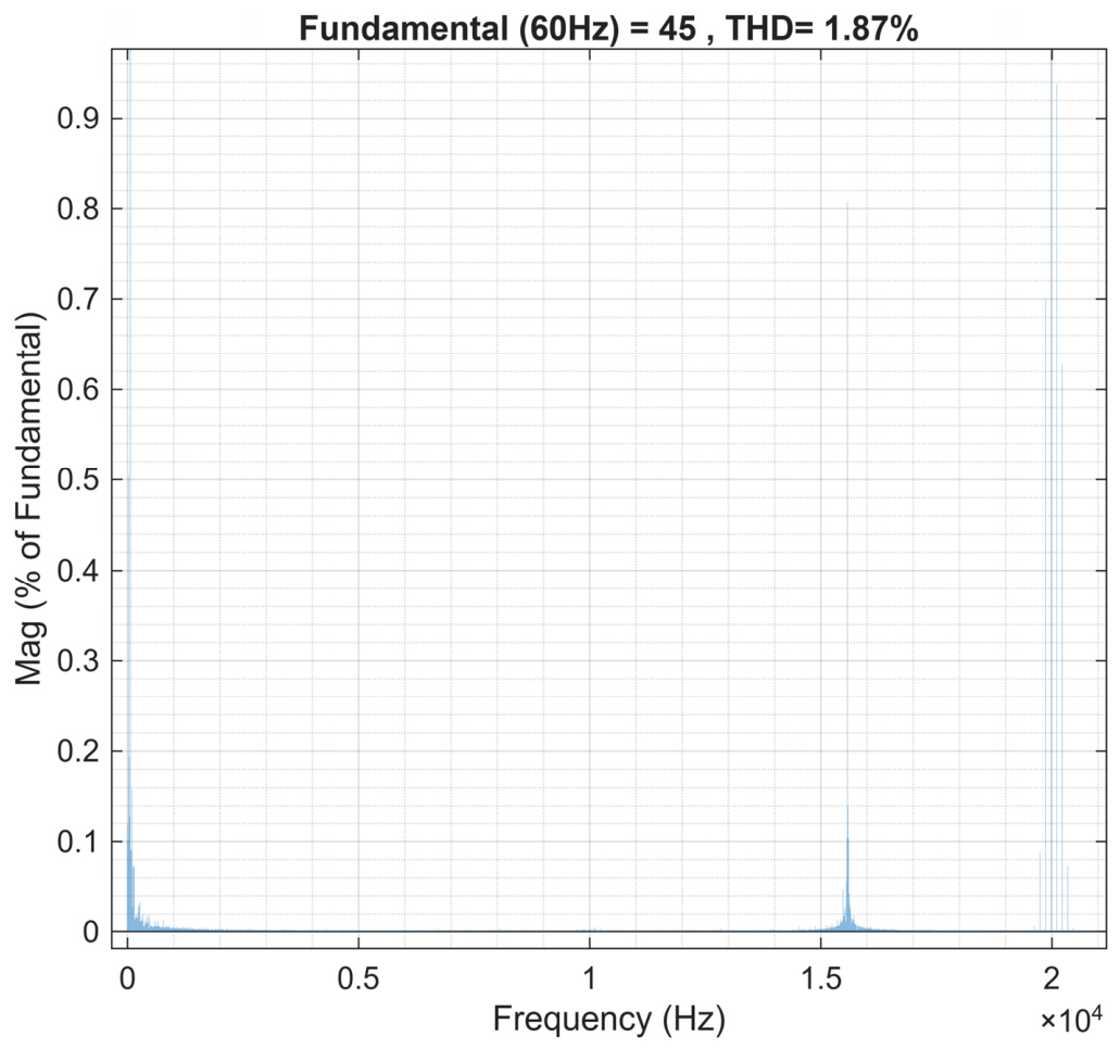
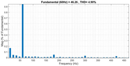
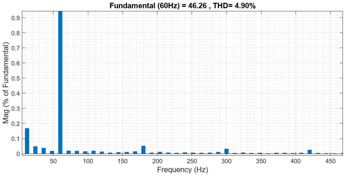
Figure 16 shows the Fast Fourier Transform (FFT) analysis of the current injected into the inverter, to evaluate its harmonic content and determine the total harmonic distortion (THD).

Figure 16. Fast Fourier Transform (FFT) and Total Harmonic Distortion (THD) in the grid current.

The fundamental component is at 60 Hz, with an amplitude of 45 A, which represents the main component of the analyzed current. In addition, high-frequency components are observed, primarily around the inverter’s switching frequency.

The THD value of 1.87% indicates that the combined contribution of the harmonic components under consideration represents a relatively low level of distortion relative to the fundamental component, thereby complying with the IEEE and IEC standards. This result suggests that the injected current has a waveform with favorable spectral quality and low harmonic content.

To validate the robustness, stability, and ability of the proposed online algorithm to reject harmonic disturbances, the system was subjected to performance tests by varying the current ripple percentage in the filtering stage. Since the quality of the power injected into the grid depends directly on the design of the coupling system, this evaluation analyzes the algorithm’s response to changes in THD.

Table 7 shows the different LCL filter values for different percentages of curl.

Table 7. Variation in current ripple percentages.

Percentage of Current Ripple	Element	Value
10%	L1	360 µH
	L2	360 µH
	Cf	0.58 µF
15%	L1	239 µH
	L2	239 µH
	Cf	0.87 µF°
20%	L1	180 µH
	L2	180 µH
	Cf	1.16 µF

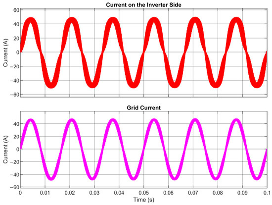
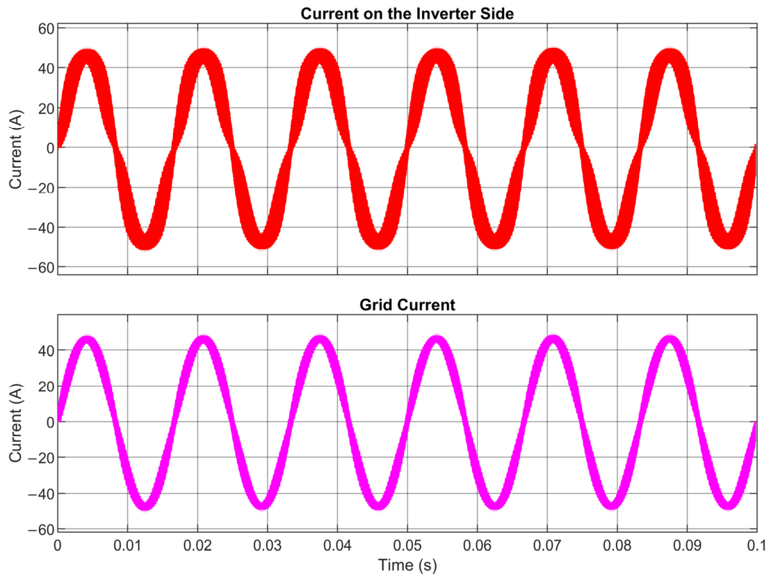
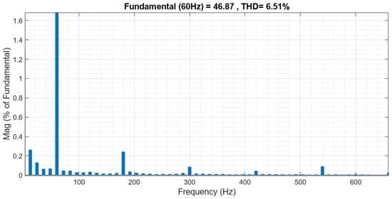
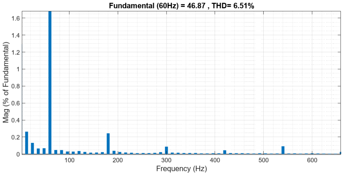
Figure 17 shows the currents on the inverter side and the grid side for a ripple percentage of 15%.

Figure 17. Grid and inverter-side current at 15% ripple.

Figure 18 shows the low-frequency harmonics for a ripple percentage of 15%.

Figure 18. Low-frequency harmonics for a 15% current ripple.

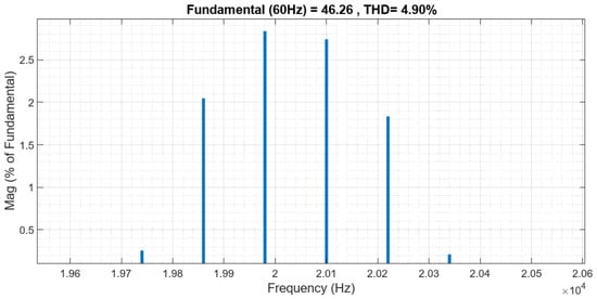
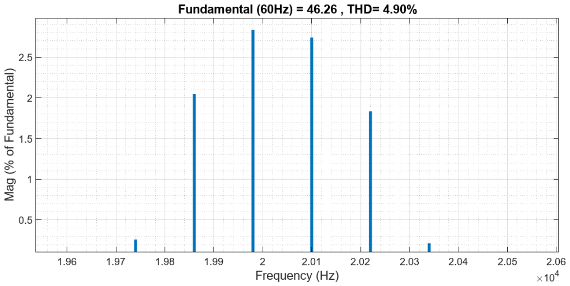
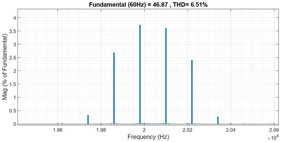
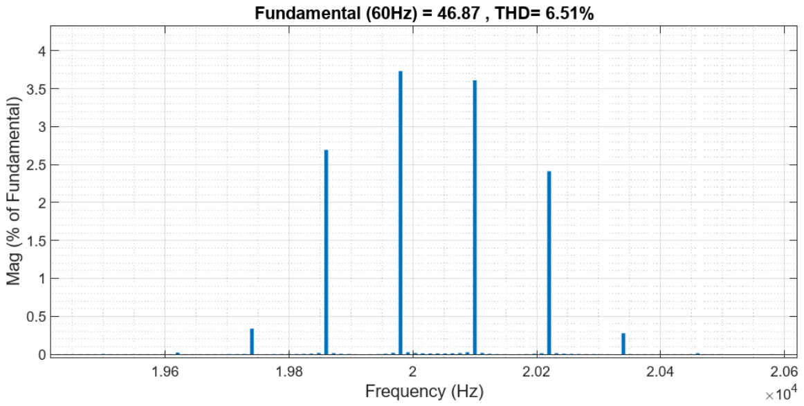
Figure 19 shows the harmonics nearly twice the switching frequency for a ripple percentage of 15%.

Figure 19. High-frequency harmonics for a 15% current ripple.

Figure 20 shows the currents on the inverter side and the grid side for a ripple per-centage of 20%.

Figure 20. Grid and inverter-side current at 20% ripple.

Figure 21 shows the low-frequency harmonics for a ripple percentage of 20%.

Figure 21. Low-frequency harmonics for a 20% current ripple.

Figure 22 shows the harmonics nearly twice the switching frequency for a ripple percentage of 20%.

Figure 22. High-frequency harmonics for a 20% current ripple.

To validate the scalability and steady-state accuracy of the proposed online algorithm, the system was tested by varying the average power injected into the power grid. This analysis verifies the correct estimation and tracking of electrical variables under different levels of power transfer.

Table 8 shows that the LCL filter values change to inject different power levels into the electrical grid.

Table 8. LCL Filter values at different average power levels.

Percentage of Current Ripple	Element	Value
1 kW	L1	2900 µH
	L2	2900 µH
	Cf	0.0721 µF
2 kW	L1	1400 µH
	L2	1400 µH
	Cf	0.14 µF°
4 kW	L1	723 µH
	L2	723 µH
	Cf	0.28 µF
16 kW	L1	180 µH
	L2	180 µH
	Cf	1.1545 µF

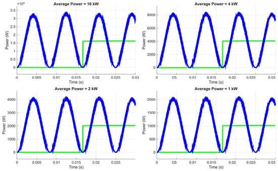
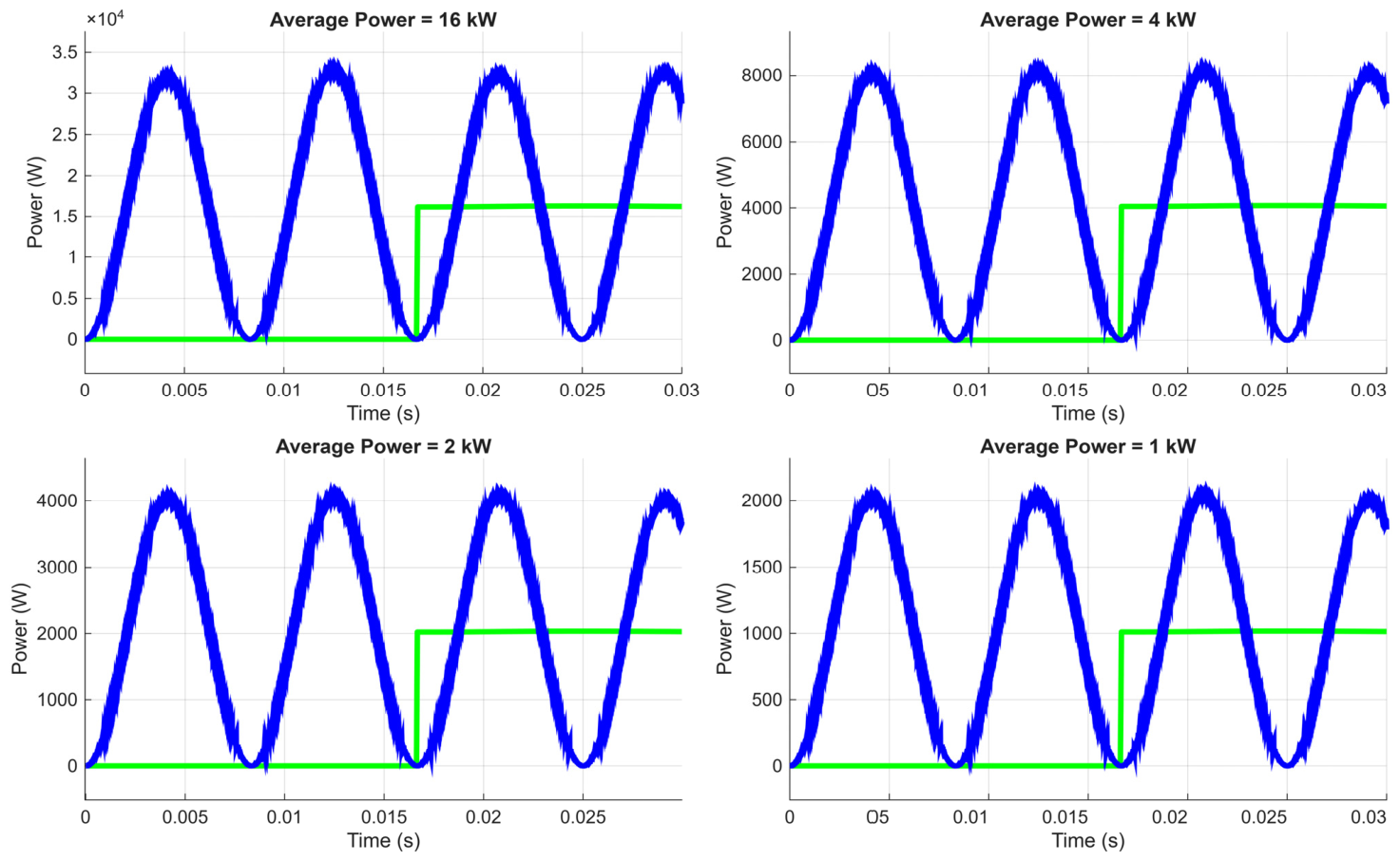
Figure 23 evaluates the performance and transient response of the proposed online algorithm for estimating average power. To validate its robustness and scalability, the algorithm was tested under four operating scenarios with different load levels: 16 kW, 4 kW, 2 kW, and 1 kW. Each of the graphs presented illustrates two main signals: Instantaneous power (blue curve) represents the oscillatory behavior of the system’s instantaneous power. This signal exhibits ripple at twice the fundamental frequency, oscillating between zero and twice the expected average power. The green signal represents the value of the average active power calculated in real time by the algorithm.

Figure 23. Online algorithm test with variable power.

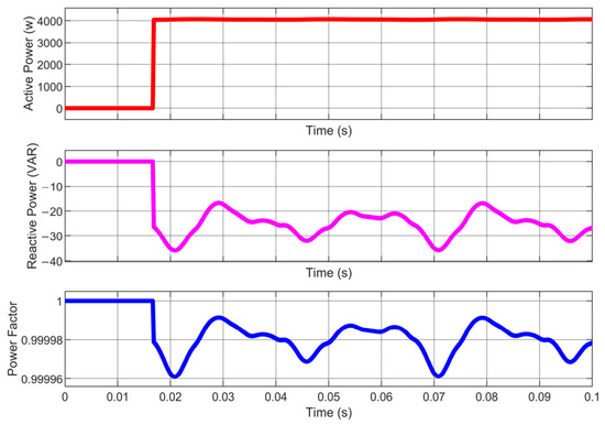
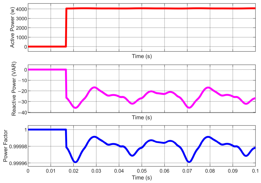
Figure 24 shows the performance of the proposed algorithm for the simultaneous, real-time calculation of power quality parameters: active power (P), reactive power (Q), and power factor (FP). The evaluation is performed over a simulation interval of 0.1 s, analyzing the estimator’s ability to extract these variables from the voltage and current signals.

Figure 24. Active power, reactive power and power factor.

The first graph (red signal) illustrates the calculation of the average active power. Consistent with previous analyses, the algorithm initializes its estimate by processing one fundamental electrical cycle. After this initial period, the signal exhibits an instantaneous dynamic response (step-like) that converges exactly to the nominal value of 4000 W. The stability of this signal in steady state is noteworthy, exhibiting a continuous trace with no perceptible ripple, which confirms excellent rejection of the oscillatory components inherent in alternating current systems.

The second graph (magenta signal) shows the reactive power injected into or absorbed by the system. As with active power, the algorithm completes its first estimate after the first cycle. From that point on, the measurement reveals a very small, capacitive reactive power injection (negative values), dynamically oscillating between −16 VAR and −36 VAR. This value is extremely low compared to the active power (4 kW), indicating a high degree of phase alignment between the voltage and the current. The ripple observed in this signal suggests the presence of minimal residual harmonic content or small transient fluctuations in the load, which the algorithm can track continuously.

The third graph (blue signal) shows the continuous calculation of the power factor. Initially set to an ideal value of one (during the calculation time of the first cycle), the PF drops transiently after the algorithm converges. However, due to the negligible magnitude of the reactive power, the calculated power factor remains exceptionally high throughout the entire simulation. The signal undergoes microvariations ranging from 0.99996 to 0.99999, directly reflecting the small perturbations observed in the reactive power graph.

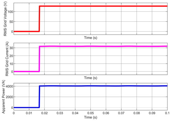
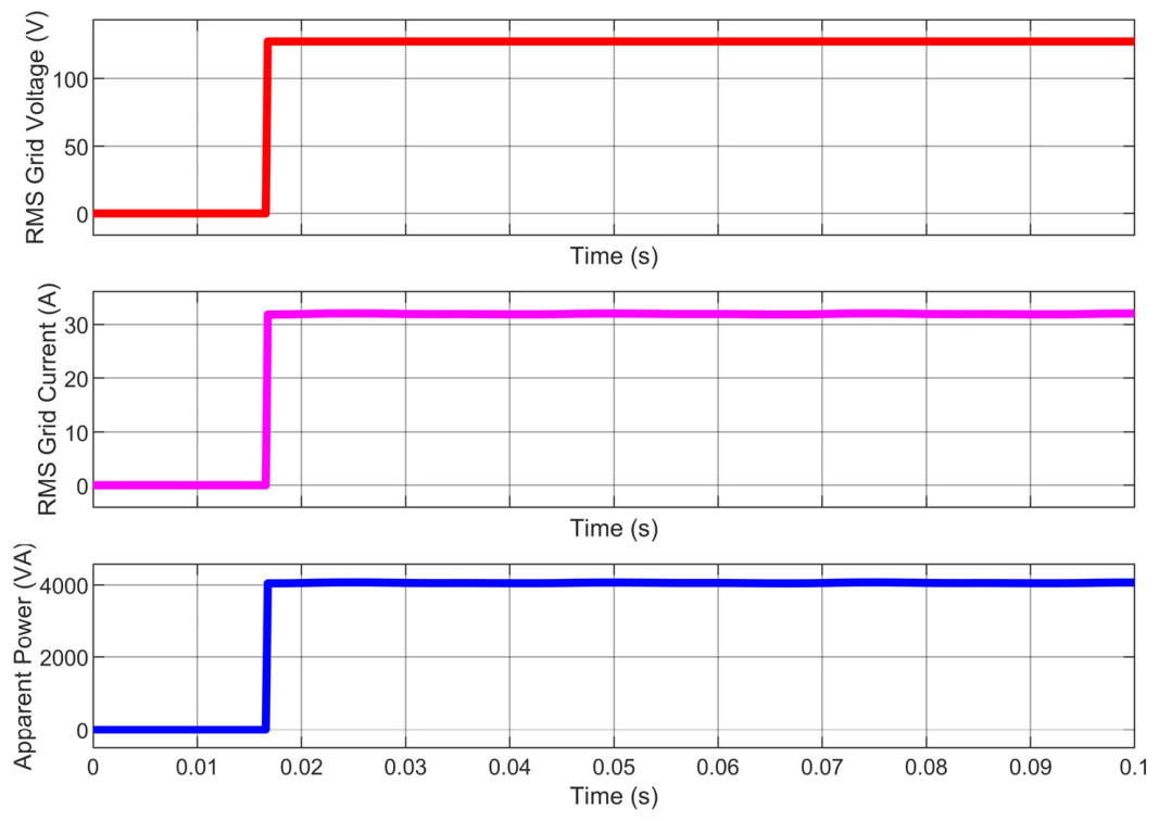
Figure 25 evaluates the performance of the proposed algorithm for the real-time calculation of the root-mean-square (RMS) values of the network variables, as well as the estimation of apparent power (S). The analysis is presented over a simulation interval of 0.1 s, demonstrating the system’s ability to extract these critical parameters from the instantaneous voltage and current waveforms.

Figure 25. RMS grid voltage, RMS grid current and apparent power.

The graph above (red signal) illustrates the dynamic calculation of the effective voltage of the power grid. The initial estimate requires sampling an entire electrical cycle. After this intrinsic latency period, the signal converges abruptly (step-like) toward its nominal value. A completely stable, ripple-free steady-state trace is observed, settling precisely at a value of approximately 127 VRMS, which is consistent with typical single-phase line voltage standards.

The central graph (magenta line) shows the estimate of the root-mean-square (RMS) value of the injected or consumed current. Exhibiting the same convergence behavior over one cycle, the estimator reaches a stable state without fluctuations. The calculated value settles at approximately 31.4 A RMS, which represents the effective magnitude of the current flowing through the system under the specified load conditions.

The graph below (blue signal) shows the real-time calculation of apparent power, which represents the total capacity of the system and is derived from the product of the previously estimated RMS values. Like the variables that make it up, the estimate of S converges after the first cycle. The steady-state signal maintains a constant and robust value of 4000 VA. The exceptional flatness of this curve confirms the algorithm’s immunity to the double-frequency oscillations typical of single-phase power systems.

3.4. Selection of Power MOSFET

To ensure the performance and efficiency of the proposed inverter, the IXFN70N120SK power transistor has been selected. This device is based on silicon carbide (SiC) technology and is specifically designed for high-power applications.

Table 9 describes the main parameters and technical characteristics that justify their selection within the developed topology.

Table 9. MOSFET parameters.

MOSFET Parameters
Parameter	Symbol	Value
Manufacturer	-	IXYS/Littelfulse®
Part number	-	IXFN70N120SK
Semiconductor material	SiC	Silicon Carbide
Drain source current direct	IDS DC	68 A
Drain source current pulsed	IDS Pulsed	170 A
Gate source voltage (ON)	VGS(on)	2.6 V
Drain source breakdown voltage	VDS	1200 V
Drain source resistance (ON)	RDS(on)	25 mΩ
Off-state conductance		2 × 10−9 S
Threshold voltage	Vth	2.6 V
Input capacitance	Ciss	2790 pF
Reverse transfer (miller) capacitance	Crss	15 pF
Output capacitance	Coss	220 pF
Turn-on delay time	td(on)	28 nS
Turn-off delay time	td(off)	125 nS

The use of the IXFN70N120SK allows for the inherent advantages of wide bandgap (WBG) devices over conventional silicon, such as lower gate charge and reduced reverse recovery times. These properties enable operation at high switching frequencies without incurring excessive energy losses.

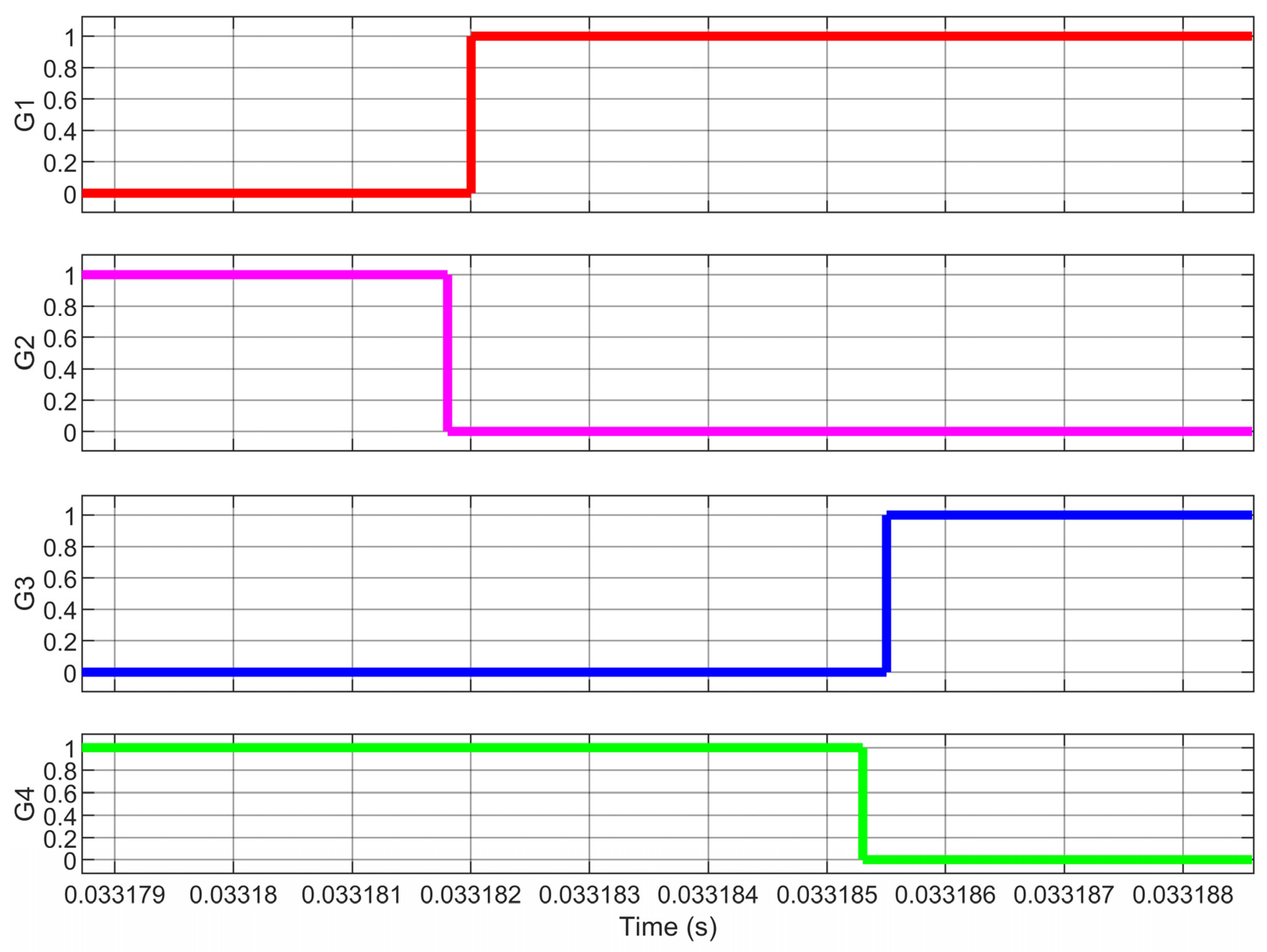
To prevent a direct short circuit in the DC link through the complementary switches of the same branch, a dead time T_d must be included in the modulation algorithm (as in the implemented unipolar SPWM scheme). This parameter defines a strict safety window during which both MOSFETs in the branch are simultaneously kept in the off state during switching transitions.

T_d > t_d(on) + t_d(off)

(48)

In the developed system, an optimized dead time in the range of 200 nsis programmed in accordance with Equation (48) and the values in Table 9, which ensures the complete turn-off of the MOSFET’s conductive channel before the complementary MOSFET begins to turn on, thereby preventing destructive transient overcurrents.

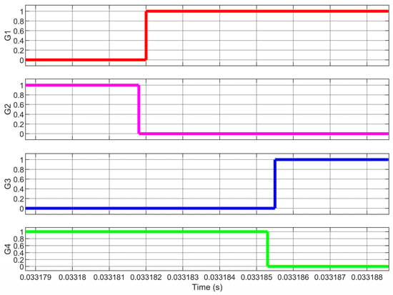
Figure 26 shows a section of the gate pulses with the programmed dead time; it can be seen that there is no signal overlap, thus preventing a possible short circuit on the DC bus.

Figure 26. Pulses at the gates with dead time.

Conduction losses occur during the interval when the transistor is fully on and carries the load current through the drain-source channel. They are modeled by the device’s resistance R_DS(on). This loss can be modeled using Equation (49):

$$P_{\mathit{cond}}=I_{D,\mathit{rms}}^2{R}_{\mathit{DS}(\mathit{on})}$$

(49)

where I_D,rms is the root-mean-square value of the current flowing through the MOSFET and R_DS(on) is the resistance. Due to the silicon carbide (SiC) technology of the IXFN70N120SK, the device has a low R_DS(on) = 34 mΩ at 25 °C which substantially reduces Joule heating compared to conventional silicon (Si) transistors.

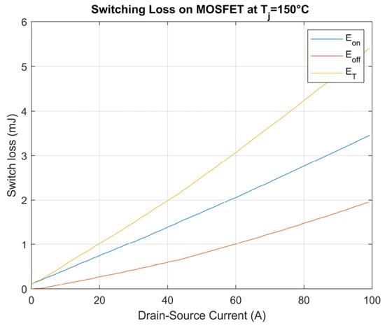
Switching losses occur during the transient intervals of transition between the off state (Off) and the on state (On), and vice versa. During these brief intervals, the voltage between the drain and source (V_DS) and the drain current (I_D) overlaps simultaneously, dissipating energy in the form of heat.

Total switching losses are the sum of the energy dissipated during the on state (E_on) and the off state (E_off), multiplied by the switching frequency (f_sw).

$$P_{\mathit{sw}}=(E_{\mathit{on}}+E_{\mathit{off}})·f_{\mathit{sw}}$$

(50)

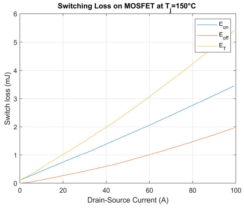
The switching losses for the selected MOSFET were plotted and are shown in Figure 27.

Figure 27. Switching loss on MOSFET.

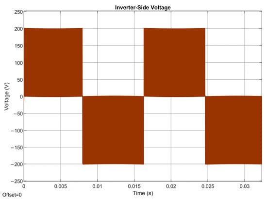
Using the values shown in Table 9, and considering switching and conduction losses as well as dead times in unipolar SPWM modulation, the MOSFET was parameterized in the Simulink simulation environment, thereby yielding a simulation that more closely resembles a SPICE model and what would be expected in experimental tests.

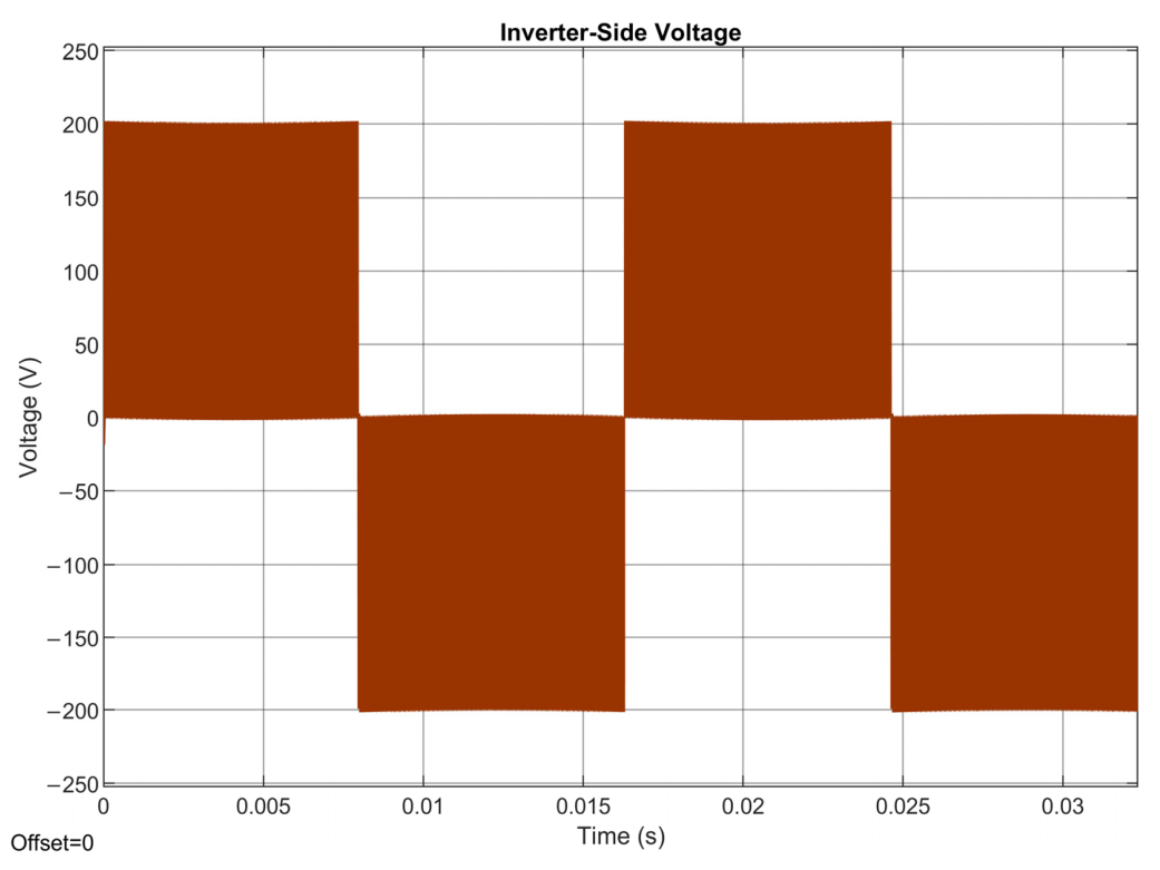
The Figure 28 shows the inverter’s output voltage with the selected MOSFET’s settings already applied.

Figure 28. Voltage of inverter side.

4. Discussion

The results obtained in this study demonstrate the technical feasibility and effectiveness of a hybrid offline–online algorithm for controlling a single-phase H-bridge inverter connected to the power grid, using unipolar SPWM modulation and LCL filtering This work could reduce the computational load and simplify the control loop. The recent literature on the control of grid-connected inverters has strongly favored the Model Predictive Control (MPC) scheme [18,19,20,21] or dynamically evaluated Space Vector Modulation (SVM) [22,23]. While these methods offer excellent transient response, they demand massive processing power, requiring high-end digital signal processors (DSPs) or field-programmable gate arrays (FPGAs) [24,25].

In contrast, the approach proposed in this paper shifts the solution of transcendental equations and the detection of crossings using Bolzano’s Theorem to an offline stage. This allows a microcontroller to be limited, in real time, to simple algebraic operations and the LUT indexing. The achieved discretization (1000 samples) guarantees switching time accuracy equivalent to or better than that of traditional analog modulators.

One of the least documented challenges in the state of the art regarding LCL filters is the inherent phase shift they introduce between the inverter voltage and the current injected into the grid. This challenge was resolved in [6] by deriving an exact mathematical expression for that phase shift; to the authors’ knowledge, this is the only article that addresses this issue.

To operate at unity power factor, most contemporary studies employ Proportional-Resonant (PR) controllers [26,27] in the steady-state αβ frame or PI controllers in the synchronous dq frame [28,29], combined with active damping techniques to suppress filter resonances.

The LCL filter design for single-phase grid-connected systems published in [30,31,32,33,34,35,36] uses the following equations. For inductor L₁, Equation (51) is used.

$$L_1={\displaystyle \frac{V_{\mathit{dc}}}{8f_{\mathit{sw}}\Delta I}}$$

(51)

where ΔI is the ripple of the current proposed. This current ripple is calculated using Equation (52).

$${\Delta }_I={\displaystyle \frac{\%r_{\mathit{inv}}\sqrt{2}{P}_{\mathit{avg}}}{100V_{g_{\mathit{rms}}}}}$$

(52)

where V_grms is the RMS grid voltage. For the inductor on the grid side, Equation (53) is used.

$$L_2=r{L}_1$$

(53)

where r is the relation between L₂ and L₁. The relation r produces values from 0 to 1. For the LCL filter capacitor, the base impedance (Z_b) is shown in Equation (54).

$$Z_b={\displaystyle \frac{{V_{g_{\mathit{rms}}}}^2}{P_{\mathit{avg}}}}$$

(54)

Z_b is used to define a base capacitance (C_b). This is shown in Equation (55).

$$C_b={\displaystyle \frac{1}{{\omega }_g{Z}_b}}$$

(55)

where ω_g is the grid angular frequency. For the calculation of the LCL filter capacitor; it is proposed that the capacitor should handle a maximum of 5% reactive power; therefore, C_b is multiplied by 0.05, as shown in Equation (56).

C_f = 0.05C_b

(56)

Equation (56) calculates the maximum value of the capacitor [32,37,38]. However, this formula is not used in this work since the aim is to minimize this value. Table 10 shows the values obtained with our equations, for average power of 4 kW and a ripple in the current of 5%.

Table 10. Reduction in the LCL filter.

Element	Valued Obtained in the Literature	Value Obtained in This Work
L1	1100 µH	725.35 µH
L2	1100 µH	725.35 µH
Cf	32.891 µF	0.2878 µF

The values of the inductors have been reduced by 34% while the capacitor is the highest reduction of 99%.

The method presented here offers an analytical feedforward alternative. By mathematically calculating the filter’s phase shift angle and integrating it directly into the phase extracted by the PLL, the system can align the injected current with the grid voltage. Simulation results demonstrate that this technique achieves a power factor of one, eliminating the need to tune complex controllers, which drastically simplifies the firmware architecture.

5. Conclusions

In this article, a hybrid offline–online algorithmic control strategy was developed and validated for injecting active power into the power grid using a single-phase full-bridge inverter with unipolar SPWM modulation and LCL filtering. The proposed methodology proved to be highly effective in ensuring synchronization with the grid, significantly reducing the complexity of the control system.

Based on the theoretical analysis and the simulation results in the Simulink environment, the following main conclusions are drawn:

The analytical pre-evaluation of switching instants (offline) based on Bolzano’s Theorem allows the firing pattern to be stored in a LUT with high temporal resolution. This could reduce the processing load on the real-time (online) controller, overcoming the computational limitations of complex dynamic methods (such as MPC or SVM) without sacrificing the precision of semiconductor switching.

The precise calculation of the intrinsic phase shift angle of the LCL filter proved to be an extremely effective phase-compensation technique. By adding this angle to the fundamental phase of the grid extracted by the PLL, the injected grid current was perfectly aligned. This made it possible to operate with a power factor of one without relying on traditional, complex closed-loop current controllers (Proportional-Resonant or PI).

The implementation of the unipolar switching technique made it possible to generate a three-level output voltage, shifting the dominant harmonic to nearly twice the switching frequency. This spectral phenomenon significantly reduced the need for passive filtering, allowing for the use of compact inductors and capacitors.

The potential reduction in the computational complexity and the physical size of the LCL filter makes this architecture highly attractive for next-generation power electronics applications, such as residential photovoltaic microinverters, energy storage systems, and bidirectional vehicle-to-grid (V2G) chargers.

In conclusion, the proposed approach strikes an optimal balance between the mathematical rigor of offline design and the agility of online execution. As a future line of work, combining this technique with wide-bandgap semiconductors (such as SiC or GaN transistors) will enable the system to scale to higher switching frequencies, power, and power density.

References

- Afonso, J.L.; Tanta, M.; Pinto, J.G.O.; Monteiro, L.F.; Machado, L.; Sousa, T.J.; Monteiro, V. A review on power electronics technologies for power quality improvement. Energies 2021, 14, 8585. [Google Scholar] [CrossRef] [Scilit]
- Rao, S.N.V.B.; Kumar, Y.V.P.; Pradeep, D.J.; Reddy, C.P.; Flah, A.; Kraiem, H.; Al-Asad, J.F. Power quality improvement in renewable-energy-based microgrid clusters using fuzzy space vector PWM controlled inverter. Sustainability 2022, 14, 4663. [Google Scholar] [CrossRef] [Scilit]
- Bhukya, M.N.; Kota, V.R.; Depuru, S.R. A simple, efficient, and novel standalone photovoltaic inverter configuration with reduced harmonic distortion. IEEE Access 2019, 7, 43831–43845. [Google Scholar] [CrossRef] [Scilit]
- Chatterjee, S.; Das, A. A review on technological aspects of different PWM techniques and its comparison based on different performance parameters. Int. J. Circuit Theory Appl. 2023, 51, 2446–2498. [Google Scholar] [CrossRef] [Scilit]
- Zhang, S.; Li, H.; Liu, Y.; Liu, X.; Lv, Q.; Du, X.; Zhang, J. An improved SPWM strategy for effectively reducing total harmonic distortion. Electronics 2024, 13, 3326. [Google Scholar] [CrossRef] [Scilit]
- Adamas-Pérez, H.; Ponce-Silva, M.; Mina-Antonio, J.D.; Claudio-Sánchez, A.; Rodríguez-Benítez, O.; Rodríguez-Benítez, O.M. A New LCL Filter Design Method for Single-Phase Photovoltaic Systems Connected to the Grid via Micro-Inverters. Technologies 2024, 12, 89. [Google Scholar] [CrossRef] [Scilit]
- Adamas-Pérez, H.; Ponce-Silva, M.; Mina-Antonio, J.D.; Claudio-Sánchez, A.; Rodríguez-Benítez, O. Assessment of Energy Conversion in Passive Components of Single-Phase Photovoltaic Systems Interconnected to the Grid. Electronics 2023, 12, 3341. [Google Scholar] [CrossRef] [Scilit]
- Raju, N.I.; Islam, M.S.; Ali, T.; Karim, S.A. Study of SPWM technique & simulation of designed analog circuit (Op-Amp) controlled three phase PWM inverter with harmonic reduction. In Proceedings of the 2013 International Conference on Informatics, Electronics and Vision (ICIEV), Dhaka, Bangladesh, 17–18 May 2013; IEEE: Washington, DC, USA, 2013; pp. 1–6. [Google Scholar]
- Samiotis, E.; Trigonidis, D.; Vokas, G.; Papageorgas, P.; Anastasiadis, A. Simulation and implementation of a SPWM inverter pulse generator circuit for educational purposes. Energy Procedia 2019, 157, 594–601. [Google Scholar] [CrossRef] [Scilit]
- Noor, S.M.; Omar, A.B.; Radzi, M.M.; Faranadia, A. Design of closed-loop algorithm of single-stage grid inverter using Digital Signal Processor (DSP) TMS320F28335 processors evaluation board. In Proceedings of the 2019 IEEE Conference on Sustainable Utilization and Development in Engineering and Technologies (CSUDET), Penang, Malaysia, 7–9 November 2019; IEEE: Piscataway, NJ, USA, 2019; pp. 290–294. [Google Scholar]
- Sarker, R.; Datta, A.; Debnath, S. FPGA-based high-definition SPWM generation with harmonic mitigation property for voltage source inverter applications. IEEE Trans. Ind. Inform. 2020, 17, 1352–1362. [Google Scholar] [CrossRef] [Scilit]
- Ponce-Silva, M.; Sánchez-Vargas, Ó.; Cortés-García, C.; Aguayo-Alquicira, J.; De León-Aldaco, S.E. Algorithm for Assessment of the Switching Angles in the Unipolar SPWM Technique for Single-Phase Inverters. Algorithms 2024, 17, 317. [Google Scholar] [CrossRef] [Scilit]
- Medina-Sánchez, M.; Yepes, A.G.; López, Ó.; Doval-Gandoy, J. Carrier phase-shift PWM with minimum stator current-ripple RMS for symmetrical six-phase induction motor drives with nearly sinusoidal winding distribution. IEEE J. Emerg. Sel. Top. Power Electron. 2025, 13, 7731–7745. [Google Scholar] [CrossRef] [Scilit]
- Cheng, J.; Xu, T.; Chen, D.; Chen, G. Dynamic and steady state response analysis of selective harmonic elimination in high power inverters. IEEE Access 2021, 9, 75588–75598. [Google Scholar] [CrossRef] [Scilit]
- Zhang, Z.; Wang, P. Research and implementation of natural sampling SPWM digital method for three-level inverter of photovoltaic power generation system based on FPGA. IEEE Access 2019, 7, 114449–114458. [Google Scholar] [CrossRef] [Scilit]
- Na, J. Design of SPWM Controller Based on FPGA. In Proceedings of the 2024 5th International Conference on Artificial Intelligence and Computer Engineering (ICAICE), Wuhu, China, 8–10 November 2024; IEEE: Piscataway, NJ, USA, 2024; pp. 1029–1032. [Google Scholar]
- Jin, X.; Li, S.; Sun, W.; Chen, W.; Gu, X.; Zhang, G. Optimized Synchronous SPWM Modulation Strategy for Traction Inverters Based on Non-Equally Spaced Carriers. World Electr. Veh. J. 2023, 14, 157. [Google Scholar] [CrossRef] [Scilit]
- Mohamed, I.S.; Rovetta, S.; Do, T.D.; Dragicević, T.; Diab, A.A.Z. A neural-network-based model predictive control of three-phase inverter with an output $ LC $ filter. IEEE Access 2019, 7, 124737–124749. [Google Scholar] [CrossRef] [Scilit]
- Scoltock, J.; Geyer, T.; Madawala, U. Model Predictive Direct Current Control for a grid-connected converter: LCL-filter versus L-filter. In Proceedings of the 2013 IEEE International Conference on Industrial Technology (ICIT), Cape Town, South Africa, 25–28 February 2013; IEEE: Piscataway, NJ, USA, 2013; pp. 576–581. [Google Scholar]
- Alharbi, Y.; Darwish, A.; Ma, X. A review of model predictive control for grid-connected PV applications. Electronics 2025, 14, 667. [Google Scholar] [CrossRef] [Scilit]
- Zheng, C.; Dragičević, T.; Zhang, Z.; Rodriguez, J.; Blaabjerg, F. Model predictive control of LC-filtered voltage source inverters with optimal switching sequence. IEEE Trans. Power Electron. 2020, 36, 3422–3436. [Google Scholar] [CrossRef] [Scilit]
- Lin, Z.; Zhang, X.; Zhu, J.; Du, W.; Ye, J.; Bai, Y. Advances in space vector modulation techniques for multilevel inverters: A comprehensive review. Chin. J. Electr. Eng. 2025, 11, 63–77. [Google Scholar] [CrossRef] [Scilit]
- Guo, X.; Du, S.; Diao, N.; Hua, C.; Blaabjerg, F. Three-dimensional space vector modulation for four-leg current-source inverters. IEEE Trans. Power Electron. 2023, 38, 13122–13132. [Google Scholar] [CrossRef] [Scilit]
- Rhouma, A.B.; Hamouda, M. Characteristics of a proposed SVPWM strategy for delta inverter with DSP-based real-time implementation. Int. Trans. Electr. Energy Syst. 2020, 30, e12384. [Google Scholar] [CrossRef] [Scilit]
- Hassaine, L.; Bengourina, M.R. Control technique for single phase inverter photovoltaic system connected to the grid. Energy Rep. 2020, 6, 200–208. [Google Scholar] [CrossRef] [Scilit]
- Husev, O.; Roncero-Clemente, C.; Makovenko, E.; Pimentel, S.P.; Vinnikov, D.; Martins, J. Optimization and implementation of the proportional-resonant controller for grid-connected inverter with significant computation delay. IEEE Trans. Ind. Electron. 2019, 67, 1201–1211. [Google Scholar] [CrossRef] [Scilit]
- Parvez, M.; Elias, M.F.M.; Abd Rahim, N.; Blaabjerg, F.; Abbott, D.; Al-Sarawi, S.F. Comparative study of discrete PI and PR controls for single-phase UPS inverter. IEEE Access 2020, 8, 45584–45595. [Google Scholar] [CrossRef] [Scilit]
- Abdolrasol, M.G.; Hannan, M.; Hussain, S.S.; Ustun, T.S. Optimal PI controller based PSO optimization for PV inverter using SPWM techniques. Energy Rep. 2022, 8, 1003–1011. [Google Scholar] [CrossRef] [Scilit]
- Arunkumar, G.; Dhanamjayulu, C.; Padmanaban, S.; Prusty, B.R.; Khan, B. Implementation of optimization-based PI controller tuning for non-ideal differential boost inverter. IEEE Access 2021, 9, 58677–58688. [Google Scholar] [CrossRef] [Scilit]
- Rasekh, N.; Hosseinpour, M. LCL filter design and robust converter side current feedback control for grid-connected Proton Exchange Membrane Fuel Cell system. Int. J. Hydrogen Energy 2020, 45, 13055–13067. [Google Scholar] [CrossRef] [Scilit]
- Sedo, J.; Kascak, S. Design of output LCL filter and control of single-phase inverter for grid-connected system. Electr. Eng. 2017, 99, 1217–1232. [Google Scholar] [CrossRef] [Scilit]
- Ruan, X.; Wang, X.; Pan, D.; Yang, D.; Li, W.; Bao, C. Control Techniques for LCL-Type Grid-Connected Inverters; Springer: Singapore, 2018. [Google Scholar]
- Ibrahim, N.F.; Mahmoud, M.M.; Al Thaiban, A.M.; Barnawi, A.B.; Elbarbary, Z.S.; Omar, A.I.; Abdelfattah, H. Operation of grid-connected PV system with ANN-based MPPT and an optimized LCL filter using GRG algorithm for enhanced power quality. IEEE Access 2023, 11, 106859–106876. [Google Scholar] [CrossRef] [Scilit]
- Arab, N.; Vahedi, H.; Al-Haddad, K. LQR control of single-phase grid-tied PUC5 inverter with LCL filter. IEEE Trans. Ind. Electron. 2019, 67, 297–307. [Google Scholar] [CrossRef] [Scilit]
- Mahlooji, M.H.; Mohammadi, H.R.; Rahimi, M. A review on modeling and control of grid-connected photovoltaic inverters with LCL filter. Renew. Sustain. Energy Rev. 2018, 81, 563–578. [Google Scholar] [CrossRef] [Scilit]
- Nagai, S.; Kusaka, K.; Itoh, J.-i. ZVRT capability of single-phase grid-connected inverter with high-speed gate-block and Minimized LCL filter design. IEEE Trans. Ind. Appl. 2018, 54, 5387–5399. [Google Scholar] [CrossRef] [Scilit]
- Said-Romdhane, M.B.; Naouar, M.W.; Belkhodja, I.S.; Monmasson, E. Simple and systematic LCL filter design for three-phase grid-connected power converters. Math. Comput. Simul. 2016, 130, 181–193. [Google Scholar] [CrossRef] [Scilit]
- Said-Romdhane, M.B.; Naouar, M.W.; Slama Belkhodja, I.; Monmasson, E. An improved LCL filter design in order to ensure stability without damping and despite large grid impedance variations. Energies 2017, 10, 336. [Google Scholar] [CrossRef] [Scilit]
Disclaimer/Publisher’s Note: The statements, opinions and data contained in all publications are solely those of the individual author(s) and contributor(s) and not of MDPI and/or the editor(s). MDPI and/or the editor(s) disclaim responsibility for any injury to people or property resulting from any ideas, methods, instructions or products referred to in the content. |
© 2026 by the authors. Licensee MDPI, Basel, Switzerland. This article is an open access article distributed under the terms and conditions of the Creative Commons Attribution (CC BY) license.