Geometric Algorithm for Optimal Quadratic Uniform Trigonometric B-Spline Interpolation Curves

Abstract

A geometric algorithm is developed for quadratic uniform trigonometric B-spline interpolation with segment-specific shape parameters. The interpolation conditions generate all control points recursively from an initial vertex. For prescribed parameters, the complete derivative calculations give a weighted initial vertex that uniquely minimizes each of the three piecewise derivative penalties. The segment-dependent weights are retained in the subsequent constrained parameter optimization. Individual and normalized weighted objectives define different choices of curve, while a consistent squared graph-error functional is used for function approximation. The geometric interpretation of the derivative penalties is distinguished from arc length, bending energy, and curvature continuity. Recomputed spatial, closed planar, and function-graph examples report objective values, interpolation and graph errors, and join diagnostics, with comparisons against polynomial constructions. The results exhibit objective-dependent trade-offs and do not establish uniform superiority or general shape preservation.

1. Introduction

B-spline curves and surfaces are fundamental representations in computer-aided geometric design [1,2]. Constructing an interpolant requires a suitable control polygon, and optimization can select one curve from the family satisfying the interpolation conditions. Related reconstruction and scattered-data procedures have been considered for dense point sets, unorganized points, interpolation–quasi-interpolation, and reverse control-point construction [3,4,5,6]. For the planar curve problem, Li et al. [7] developed quadratic uniform B-spline interpolation with an optimized endpoint condition.

Shape parameters provide additional flexibility in polynomial and trigonometric representations. Extensions of quadratic uniform B-spline curves were investigated in [8], while B-spline-based path planning and algebraic tensor-product surface modeling provide application contexts [9,10]. Piecewise quadratic trigonometric polynomial curves [11], trigonometric B-spline representations [12], constrained geometric-continuity interpolation [13], adjustable trigonometric B-splines [14] and uniform trigonometric polynomial B-splines [15] motivate the present curve family. The choice of a trigonometric basis alone, however, does not guarantee improved accuracy or periodic interpolation.

Optimization criteria for B-spline and Hermite interpolation include internal-energy formulations [16], point-normal interpolation with minimal energy [17], length and curvature-variation objectives [18], and derivative-oscillation and strain criteria [19]. Cardinal-spline shape optimization is another related topic [20]. Xie et al. [21], building on the endpoint construction in [7], studied recurrent control-point generation for quadratic uniform polynomial B-splines with parameters. In using such objectives, the parameterization and the exact functional must be stated: an integral of a squared parameter derivative generally differs from a geometric length or curvature functional.

Recent international studies further distinguish specified shape constraints from visual smoothness. Shape-preserving surface interpolation [22], positivity- and monotonicity-preserving trigonometric interpolation [23], and point-normal convexity-preserving interpolation [24] formulate particular geometric requirements. The derivative-penalty optimization studied here does not automatically guarantee monotonicity, convexity, or absence of overshoot; corresponding geometric constraints are required when these properties are needed.

The present work extends the recurrent control-point approach to the quadratic uniform trigonometric family. Its main result is a parameter-dependent weighted initial vertex and its conditional optimality for prescribed segment parameters. The full first-, second-, and third-derivative calculations are given separately. Section 1 defines the interpolation curve. Section 2 derives the control-point algorithm. Section 3 optimizes the segment parameters and reports the spatial and planar examples. Section 4 formulates graph approximation and recomputes the function example. Section 5 states the conclusions and limitations.

2. Quadratic Uniform Trigonometric B-Spline Interpolation Curve

Definition 1. 

Let p₀,…,p_n ∈ ℝ^d, where d = 2 or d = 3 and n ≥ 2 are control vertices. The curve consists of n − 1 segments, each using a unit local parameter interval:

r_i(t) = b_0,2(t,α_i)p_i + b_1,2(t,α_i)p_i+1 + b_2,2(t,α_i)p_i+2, 0 ≤ t ≤ 1,

(1)

Here, i = 0,…,n − 2, and the three basis functions are

$$\begin{array}{l}{b}_{0,2}(t,{\alpha }_i)={\displaystyle \frac{1}{2}}\left(1-\sin {\displaystyle \frac{\mathit{\pi t}}{2}}\right)\left(1-{\alpha }_i\sin {\displaystyle \frac{\mathit{\pi t}}{2}}\right),\hfill \\ b_{1,2}(t,{\alpha }_i)={\displaystyle \frac{1}{2}}\left[-{\alpha }_i+(1+{\alpha }_i)\left(\sin {\displaystyle \frac{\mathit{\pi t}}{2}}+\cos {\displaystyle \frac{\mathit{\pi t}}{2}}\right)\right],\hfill \\ b_{2,2}(t,{\alpha }_i)={\displaystyle \frac{1}{2}}\left(1-\cos {\displaystyle \frac{\mathit{\pi t}}{2}}\right)\left(1-{\alpha }_i\cos {\displaystyle \frac{\mathit{\pi t}}{2}}\right).\hfill \end{array}$$

(2)

The admissible shape parameters satisfy −1 < α_i ≤ 1. For these parameters, the basis functions are nonnegative and satisfy b_0,2 + b_1,2 + b_2,2 = 1. Their endpoint values and derivatives give

$$r_i(0)={\displaystyle \frac{1}{2}}(p_i+p_{i+1}),\hspace{1em}\hspace{1em}{r}_i(1)={\displaystyle \frac{1}{2}}(p_{i+1}+p_{i+2}),$$

(3)

$$\begin{array}{l}{r}_i^{\prime }(0)={\displaystyle \frac{\pi }{4}}(1+{\alpha }_i)(p_{i+1}-p_i),\hfill \\ r_i^{\prime }(1)={\displaystyle \frac{\pi }{4}}(1+{\alpha }_i)(p_{i+2}-p_{i+1}).\hfill \end{array}$$

(4)

To interpolate the ordered data d₁,…,d_n ∈ ℝ^d, impose the midpoint conditions

$$d_i={\displaystyle \frac{1}{2}}(p_{i-1}+p_i),\hspace{1em}\hspace{1em}i=1,\dots ,n.$$

(5)

At an interior join, the endpoint derivatives are positive multiples of the shared control edge. Thus, the join is G¹ when that edge is nonzero. Equal adjacent parameters additionally give C¹ continuity for the unit local intervals. A zero shared edge produces zero endpoint derivatives and requires a separate regularity analysis. Neither G¹ nor C¹ implies continuity of curvature. Repeated end data only enforce positional closure and do not guarantee tangent alignment at the closing seam.

3. Algorithm for Generating Control Points

Given the initial vertex p₀, Equation (5) yields all remaining control vertices recursively:

p_i = 2d_i − p_i−1,  i = 1,…,n.

(6)

Repeated substitution gives the complete alternating-sum expression

$$p_i={(-1)}^i{p}_0+2{\displaystyle \sum _{j=1}^i{(-1)}^{i-j}}{d}_j,\hspace{1em}\hspace{1em}i=1,\dots ,n.$$

(7)

The explicit sum is useful in the proofs. Computation uses Equation (6) so that earlier partial sums are not recomputed. We select the initial vertex using parameter-dependent derivative penalties. These are integrated separately over each segment and do not include jump penalties at joins.

3.1. Selecting Control Points by Minimizing the First-Derivative Penalty

Substituting the two midpoint recurrences into Equation (1) gives the expanded segment expression

$$\begin{array}{l}{r}_i(t)=(1+{\alpha }_i)\left(1-\sin {\displaystyle \frac{\mathit{\pi t}}{2}}-\cos {\displaystyle \frac{\mathit{\pi t}}{2}}\right)p_i\hfill \\ \hspace{1em}+\left[(1+{\alpha }_i)\left(\sin {\displaystyle \frac{\mathit{\pi t}}{2}}+2\cos {\displaystyle \frac{\mathit{\pi t}}{2}}-1\right)-{\alpha }_i{\cos }^2{\displaystyle \frac{\mathit{\pi t}}{2}}\right]d_{i+1}\hfill \\ \hspace{1em}+\left[1-(1+{\alpha }_i)\cos {\displaystyle \frac{\mathit{\pi t}}{2}}+{\alpha }_i{\cos }^2{\displaystyle \frac{\mathit{\pi t}}{2}}\right]d_{i+2}.\hfill \end{array}$$

(8)

Differentiating every coefficient in Equation (8) gives

$$\begin{array}{l}{r}_i^{\prime }(t)={\displaystyle \frac{\pi }{2}}(1+{\alpha }_i)\left(\sin {\displaystyle \frac{\mathit{\pi t}}{2}}-\cos {\displaystyle \frac{\mathit{\pi t}}{2}}\right)p_i\hfill \\ \hspace{1em}+\left[{\displaystyle \frac{\pi }{2}}(1+{\alpha }_i)\left(\cos {\displaystyle \frac{\mathit{\pi t}}{2}}-2\sin {\displaystyle \frac{\mathit{\pi t}}{2}}\right)+{\displaystyle \frac{\pi {\alpha }_i}{2}}\sin (\mathit{\pi t})\right]d_{i+1}\hfill \\ \hspace{1em}+\left[{\displaystyle \frac{\pi }{2}}(1+{\alpha }_i)\sin {\displaystyle \frac{\mathit{\pi t}}{2}}-{\displaystyle \frac{\pi {\alpha }_i}{2}}\sin (\mathit{\pi t})\right]d_{i+2}.\hfill \end{array}$$

(9)

The first-derivative penalty is, therefore,

$$\begin{array}{l}{E}_1(p_0,\alpha )={\displaystyle {\displaystyle \sum _{i=0}^{n-2}}{\displaystyle {\displaystyle \underset{0}{\overset{1}{\int }}}\Vert r_i^{\prime }(t){\Vert }^2}}\mathit{dt}\hfill \\ \hspace{1em}={\displaystyle \sum _{i=0}^{n-2}{\displaystyle {\displaystyle \underset{0}{\overset{1}{\int }}}{‖\begin{array}{l}\frac{\pi }{2}(1+{\alpha }_i)\left(\sin \frac{\mathit{\pi t}}{2}-\cos \frac{\mathit{\pi t}}{2}\right)p_i\hfill \\ \hspace{1em}+\left[\frac{\pi }{2}(1+{\alpha }_i)\left(\cos \frac{\mathit{\pi t}}{2}-2\sin \frac{\mathit{\pi t}}{2}\right)+\frac{\pi {\alpha }_i}{2}\sin (\mathit{\pi t})\right]d_{i+1}\hfill \\ \hspace{1em}+\left[\frac{\pi }{2}(1+{\alpha }_i)\sin \frac{\mathit{\pi t}}{2}-\frac{\pi {\alpha }_i}{2}\sin (\mathit{\pi t})\right]d_{i+2}\hfill \end{array}‖}^2}}\mathit{dt}.\hfill \end{array}$$

(10)

Lemma 1. 

If u(1 − t) = u(t) and v(1 − t) = −v(t), then ${\displaystyle {\displaystyle \underset{0}{\overset{1}{\int }}}u}(t)v(t)\mathit{dt}=0$. Their derivatives of the same order also have opposite parity.

Proof. 

The substitution t ↦ 1 − t changes the sign of the integral without changing its value, so it is zero. Differentiating the symmetry identities proves the derivative statement. □

Applying Lemma 1 after substitution of Equation (7) and evaluating the trigonometric integrals, this exactly gives the complete quadratic expression

$$\begin{array}{l}{E}_1={\displaystyle \sum _{i=0}^{n-2}\left[\left(\frac{\pi (\pi +2)}{16}+2\frac{\pi (3\pi -10)}{48}{\alpha }_i+\frac{\pi (9\pi -26)}{48}{\alpha }_i^2\right)\Vert d_{i+2}-d_{i+1}{\Vert }^2\right.}\hfill \\ \hspace{1em}\hspace{1em}\left.+{\displaystyle \frac{\pi (\pi -2)}{4}}{(1+{\alpha }_i)}^2{‖p_0-{(-1)}^i\left({\displaystyle \frac{3d_{i+1}-d_{i+2}}{2}}-2{\displaystyle \sum _{j=1}^i{(-1)}^{i-j}}{d}_j\right)‖}^2\right].\hfill \end{array}$$

(11)

Theorem 1. 

For fixed admissible parameters α = (α₀,…,α_n−2), the unique initial vertex minimizing E₁ is

$$p_0^{*}(\alpha )={\displaystyle \frac{{\displaystyle \sum _{i=0}^{n-2}{(-1)}^i}{(1+{\alpha }_i)}^2\left[\frac{3d_{i+1}-d_{i+2}}{2}-2{\displaystyle \sum _{j=1}^i{(-1)}^{i-j}}{d}_j\right]}{{\displaystyle \sum _{i=0}^{n-2}{(1+{\alpha }_i)}^2}}}.$$

(12)

Proof. 

For n = 2, differentiation of Equation (11) gives

$${\nabla }_{p_0}{E}_1=2{\displaystyle \frac{\pi (\pi -2)}{4}}{(1+{\alpha }_0)}^2\left(p_0-{\displaystyle \frac{3d_1-d_2}{2}}\right).$$

(13)

Thus, $p_0^{*}=(3d_1-d_2)/2$. For n > 2, retaining each segment weight inside the summation gives

$$\begin{array}{l}{\nabla }_{p_0}{E}_1=2{\displaystyle \frac{\pi (\pi -2)}{4}}{\displaystyle \sum _{i=0}^{n-2}{(1+{\alpha }_i)}^2}\hfill \\ \hspace{1em}\hspace{1em}\cdot \left[p_0-{(-1)}^i\left({\displaystyle \frac{3d_{i+1}-d_{i+2}}{2}}-2{\displaystyle \sum _{j=1}^i{(-1)}^{i-j}}{d}_j\right)\right].\hfill \end{array}$$

(14)

$${\nabla }_{p_0}^2{E}_1={\displaystyle \frac{\pi (\pi -2)}{2}}\left[{\displaystyle \sum _{i=0}^{n-2}{(1+{\alpha }_i)}^2}\right]I_d\succ 0.$$

(14a)

Setting Equation (14) to zero yields Equation (12), and the positive-definite Hessian proves uniqueness. For equal parameters, the weights cancel, but for unequal parameters they cannot be removed. Empty sums are zero throughout. The dependence of $p_0^{*}$ on the complete parameter vector is retained in Algorithm 2. □

For the counterexample d₁ = (0, 0), d₂ = (1, 1), d₃ = (2, 0), α₀ = 0 and α₁ = 1, Equation (12) gives $p_0^{*}=(-0.5,-1.3)$ and E₁ = 4.90259808. The unweighted vertex (−0.5, −1) gives E₁ = 5.30607023, confirming that removing the individual weights changes the minimizer.

3.2. Selecting Control Points by Minimizing the Second-Derivative Penalty

Differentiating Equation (9) gives the full second derivative

$$\begin{array}{l}{r}_i^{″}(t)={\displaystyle \frac{{\pi }^2}{4}}(1+{\alpha }_i)\left(\cos {\displaystyle \frac{\mathit{\pi t}}{2}}+\sin {\displaystyle \frac{\mathit{\pi t}}{2}}\right)p_i\hfill \\ \hspace{1em}+\left[-{\displaystyle \frac{{\pi }^2}{4}}(1+{\alpha }_i)\left(\sin {\displaystyle \frac{\mathit{\pi t}}{2}}+2\cos {\displaystyle \frac{\mathit{\pi t}}{2}}\right)+{\displaystyle \frac{{\pi }^2{\alpha }_i}{2}}\cos (\mathit{\pi t})\right]d_{i+1}\hfill \\ \hspace{1em}+\left[{\displaystyle \frac{{\pi }^2}{4}}(1+{\alpha }_i)\cos {\displaystyle \frac{\mathit{\pi t}}{2}}-{\displaystyle \frac{{\pi }^2{\alpha }_i}{2}}\cos (\mathit{\pi t})\right]d_{i+2}.\hfill \end{array}$$

(15)

The corresponding squared-derivative integral and its evaluated form are

$$E_2={\displaystyle \sum _{i=0}^{n-2}{\displaystyle {\displaystyle \underset{0}{\overset{1}{\int }}}{‖\begin{array}{l}\frac{{\pi }^2}{4}(1+{\alpha }_i)\left(\cos \frac{\mathit{\pi t}}{2}+\sin \frac{\mathit{\pi t}}{2}\right)p_i\hfill \\ \hspace{1em}+\left[-\frac{{\pi }^2}{4}(1+{\alpha }_i)\left(\sin \frac{\mathit{\pi t}}{2}+2\cos \frac{\mathit{\pi t}}{2}\right)+\frac{{\pi }^2{\alpha }_i}{2}\cos (\mathit{\pi t})\right]d_{i+1}\hfill \\ \hspace{1em}+\left[\frac{{\pi }^2}{4}(1+{\alpha }_i)\cos \frac{\mathit{\pi t}}{2}-\frac{{\pi }^2{\alpha }_i}{2}\cos (\mathit{\pi t})\right]d_{i+2}\hfill \end{array}‖}^2}}\mathit{dt}.$$

(16)

$$\begin{array}{l}{E}_2={\displaystyle \sum _{i=0}^{n-2}\left[\left(\frac{{\pi }^3(\pi -2)}{64}+2\frac{{\pi }^3(3\pi -22)}{192}{\alpha }_i+\frac{{\pi }^3(27\pi -38)}{192}{\alpha }_i^2\right)\Vert d_{i+2}-d_{i+1}{\Vert }^2\right.}\hfill \\ \hspace{1em}\hspace{1em}\left.+{\displaystyle \frac{{\pi }^3(\pi +2)}{16}}{(1+{\alpha }_i)}^2{‖p_0-{(-1)}^i\left({\displaystyle \frac{3d_{i+1}-d_{i+2}}{2}}-2{\displaystyle \sum _{j=1}^i{(-1)}^{i-j}}{d}_j\right)‖}^2\right].\hfill \end{array}$$

(16a)

Theorem 2. 

For fixed admissible segment parameters, the initial vertex in Equation (12) uniquely minimizes E₂.

Proof. 

For n = 2, the derivative is

$${\nabla }_{p_0}{E}_2=2{\displaystyle \frac{{\pi }^3(\pi +2)}{16}}{(1+{\alpha }_0)}^2\left(p_0-{\displaystyle \frac{3d_1-d_2}{2}}\right).$$

(17)

For n > 2, the complete weighted derivative is

$$\begin{array}{l}{\nabla }_{p_0}{E}_2=2{\displaystyle \frac{{\pi }^3(\pi +2)}{16}}{\displaystyle \sum _{i=0}^{n-2}{(1+{\alpha }_i)}^2}\hfill \\ \hspace{1em}\hspace{1em}\cdot \left[p_0-{(-1)}^i\left({\displaystyle \frac{3d_{i+1}-d_{i+2}}{2}}-2{\displaystyle \sum _{j=1}^i{(-1)}^{i-j}}{d}_j\right)\right].\hfill \end{array}$$

(18)

$${\nabla }_{p_0}^2{E}_2={\displaystyle \frac{{\pi }^3(\pi +2)}{8}}\left[{\displaystyle \sum _{i=0}^{n-2}{(1+{\alpha }_i)}^2}\right]I_d\succ 0.$$

(18a)

The zero-gradient equation again yields Equation (12), and the Hessian proves uniqueness. This conclusion fixes the parameters; it does not assert that the same parameters minimize E₁ and E₂. □

3.3. Selecting Control Points by Minimizing the Third-Derivative Penalty

One further differentiation gives

$$\begin{array}{l}{r}_i^{‴}(t)={\displaystyle \frac{{\pi }^3}{8}}(1+{\alpha }_i)\left(\cos {\displaystyle \frac{\mathit{\pi t}}{2}}-\sin {\displaystyle \frac{\mathit{\pi t}}{2}}\right)p_i\hfill \\ \hspace{1em}+\left[{\displaystyle \frac{{\pi }^3}{8}}(1+{\alpha }_i)\left(2\sin {\displaystyle \frac{\mathit{\pi t}}{2}}-\cos {\displaystyle \frac{\mathit{\pi t}}{2}}\right)-{\displaystyle \frac{{\pi }^3{\alpha }_i}{2}}\sin (\mathit{\pi t})\right]d_{i+1}\hfill \\ \hspace{1em}+\left[-{\displaystyle \frac{{\pi }^3}{8}}(1+{\alpha }_i)\sin {\displaystyle \frac{\mathit{\pi t}}{2}}+{\displaystyle \frac{{\pi }^3{\alpha }_i}{2}}\sin (\mathit{\pi t})\right]d_{i+2}.\hfill \end{array}$$

(19)

Thus, the third-derivative penalty is

$$E_3={\displaystyle \sum _{i=0}^{n-2}{\displaystyle {\displaystyle \underset{0}{\overset{1}{\int }}}{‖\begin{array}{l}\frac{{\pi }^3}{8}(1+{\alpha }_i)\left(\cos \frac{\mathit{\pi t}}{2}-\sin \frac{\mathit{\pi t}}{2}\right)p_i\hfill \\ \hspace{1em}+\left[\frac{{\pi }^3}{8}(1+{\alpha }_i)\left(2\sin \frac{\mathit{\pi t}}{2}-\cos \frac{\mathit{\pi t}}{2}\right)-\frac{{\pi }^3{\alpha }_i}{2}\sin (\mathit{\pi t})\right]d_{i+1}\hfill \\ \hspace{1em}+\left[-\frac{{\pi }^3}{8}(1+{\alpha }_i)\sin \frac{\mathit{\pi t}}{2}+\frac{{\pi }^3{\alpha }_i}{2}\sin (\mathit{\pi t})\right]d_{i+2}\hfill \end{array}‖}^2}}\mathit{dt}.$$

(20)

$$\begin{array}{l}{E}_3={\displaystyle \sum _{i=0}^{n-2}\left[\left(\frac{{\pi }^5(\pi +2)}{256}+2\frac{{\pi }^5(3\pi -58)}{768}{\alpha }_i+\frac{{\pi }^5(99\pi -122)}{768}{\alpha }_i^2\right)\Vert d_{i+2}-d_{i+1}{\Vert }^2\right.}\hfill \\ \hspace{1em}\hspace{1em}\left.+{\displaystyle \frac{{\pi }^5(\pi -2)}{64}}{(1+{\alpha }_i)}^2{‖p_0-{(-1)}^i\left({\displaystyle \frac{3d_{i+1}-d_{i+2}}{2}}-2{\displaystyle \sum _{j=1}^i{(-1)}^{i-j}}{d}_j\right)‖}^2\right].\hfill \end{array}$$

(20a)

Theorem 3. 

For fixed admissible segment parameters, the initial vertex in Equation (12) uniquely minimizes E₃.

Proof. 

For n = 2,

$${\nabla }_{p_0}{E}_3=2{\displaystyle \frac{{\pi }^5(\pi -2)}{64}}{(1+{\alpha }_0)}^2\left(p_0-{\displaystyle \frac{3d_1-d_2}{2}}\right).$$

(21)

For n > 2, differentiation of the evaluated penalty gives

$$\begin{array}{l}{\nabla }_{p_0}{E}_3=2{\displaystyle \frac{{\pi }^5(\pi -2)}{64}}{\displaystyle \sum _{i=0}^{n-2}{(1+{\alpha }_i)}^2}\hfill \\ \hspace{1em}\hspace{1em}\cdot \left[p_0-{(-1)}^i\left({\displaystyle \frac{3d_{i+1}-d_{i+2}}{2}}-2{\displaystyle \sum _{j=1}^i{(-1)}^{i-j}}{d}_j\right)\right].\hfill \end{array}$$

(22)

$${\nabla }_{p_0}^2{E}_3={\displaystyle \frac{{\pi }^5(\pi -2)}{32}}\left[{\displaystyle \sum _{i=0}^{n-2}{(1+{\alpha }_i)}^2}\right]I_d\succ 0.$$

(22a)

The stationary vertex is Equation (12), and it is unique. Different penalties generally produce different optimized parameter vectors and hence different final control polygons. □

Geometric interpretation: The quantities E₁, E₂ and E₃ depend on the chosen parameterization. For regular curves, geometric length and bending energy are instead

$$\begin{array}{l}L={\displaystyle {\displaystyle \sum _{i=0}^{n-2}}{\displaystyle {\displaystyle \underset{0}{\overset{1}{\int }}}\Vert r_i^{\prime }(t)\Vert }}\mathit{dt},\hspace{1em}\hspace{1em}B={\displaystyle {\displaystyle \sum _{i=0}^{n-2}}{\displaystyle {\displaystyle \underset{0}{\overset{1}{\int }}}{\kappa }_i}}{(t)}^2\Vert r_i^{\prime }(t)\mathit{dt}\Vert ,\hfill \\ {\kappa }_i(t)={\displaystyle \frac{\sqrt{\Vert r_i^{\prime }{\Vert }^2\Vert r_i^{″}{\Vert }^2-{(r_i^{\prime }\cdot r_i^{\prime \prime })}^2}}{\Vert r_i^{\prime }{\Vert }^3}}.\hfill \end{array}$$

(22b)

Under unit-speed arc-length parameterization, the first two squared-derivative integrals reduce to length and bending energy. No such assumption is made here. Even under unit speed, the third-derivative integral generally contains additional curvature terms and is not merely ${\displaystyle \int {(\mathit{d\kappa }/\mathit{ds})}^2}\mathit{ds}$. Segment-wise penalties do not ensure curvature continuity at joins. Length, bending energy and one-sided curvature jumps are therefore evaluated separately in the examples.

The complete procedure for generating control points under fixed given segment-wise shape parameters is summarized in Algorithm 1.

Algorithm 1. Generating control points for prescribed parameters

Step 1. Input d1,…,dn and admissible α0,…,αn−2. Step 2. Evaluate the numerator and denominator of Equation (12). Maintain the alternating offsets using p0 = 0 and pi+1 = 2di+1 − pi, rather than recomputing the inner sums. Step 3. Starting from $p_0^{*}$, generate the remaining vertices by Equation (6). Check the midpoint interpolation residuals and nonzero shared control edges. Construction and storage cost O(nd), where d is the coordinate dimension.

4. Derivative-Penalty-Minimizing Interpolation Curves

The initial vertex in Equation (12) depends on the segment parameters. Therefore, selecting it once and then changing the parameters does not solve the joint problem. The following individual formulas describe conditional minimization with p₀ fixed. Algorithm 2 instead substitutes $p_0^{*}(\alpha )$ at every trial vector.

The theoretical interval (−1, 1] has an open lower endpoint; an infimum may be approached without being attained. Numerical optimization uses [−1 + ε, 1], with ε = 10⁻⁴ unless otherwise stated. This restriction is explicitly included in all reported numerical results.

4.1. First-Derivative-Penalty-Minimizing Interpolation Curve

For the first-derivative criterion, the joint regularized problem is

$${\min }_{\alpha \in {[-1+\epsilon ,1]}^{n-1}}{E}_1(p_0^{*}(\alpha ),\alpha ).$$

(23)

For a fixed initial vertex, differentiating the complete quadratic penalty with respect to α_i and setting the derivative to zero gives the following unconstrained stationary value. The numerator and denominator are written out separately to retain every term at a readable size:

$$\begin{array}{l}{\alpha }_{i,\mathrm{unc}}^{(1)}=-{\displaystyle \frac{N_{1,i}}{Q_{1,i}}},\hfill \\ N_{1,i}={\displaystyle \frac{\pi (3\pi -10)}{48}}\Vert d_{i+2}-d_{i+1}{\Vert }^2+{\displaystyle \frac{\pi (\pi -2)}{4}}{‖p_0-{(-1)}^i\left({\displaystyle \frac{3d_{i+1}-d_{i+2}}{2}}-2{\displaystyle \sum _{j=1}^i{(-1)}^{i-j}}{d}_j\right)‖}^2,\hfill \\ Q_{1,i}={\displaystyle \frac{\pi (9\pi -26)}{48}}\Vert d_{i+2}-d_{i+1}{\Vert }^2+{\displaystyle \frac{\pi (\pi -2)}{4}}{‖p_0-{(-1)}^i\left({\displaystyle \frac{3d_{i+1}-d_{i+2}}{2}}-2{\displaystyle \sum _{j=1}^i{(-1)}^{i-j}}{d}_j\right)‖}^2.\hfill \end{array}$$

(24)

$$\begin{array}{l}{\alpha }_i^{(k)}=\min \left\{1,\max \left\{-1+\epsilon ,-{\displaystyle \frac{N_{k,i}}{Q_{k,i}}}\right\}\right\},\hspace{1em}\hspace{1em}{Q}_{k,i}>0,\hfill \\ {\alpha }_i^{(k)}=0,\hspace{1em}\hspace{1em}{Q}_{k,i}=0,\hspace{1em}\hspace{1em}k=1,2,3.\hfill \end{array}$$

(24a)

The projection explicitly includes upper and lower boundary solutions. The constants multiplying both squared norms in Q_k,i are positive. Thus, a zero denominator means both norms vanish, the segment is constant, and every admissible parameter gives the same penalty; zero is selected deterministically. A scale-aware tolerance is needed in floating-point implementations. The excluded value −1 is never accepted as a feasible parameter.

4.2. Second-Derivative-Penalty-Minimizing Interpolation Curve

For the second-derivative criterion, the joint regularized problem is

$${\min }_{\alpha \in {[-1+\epsilon ,1]}^{n-1}}{E}_2(p_0^{*}(\alpha ),\alpha ).$$

(25)

Given a fixed initial vertex, differentiating the complete quadratic penalty with respect to α_i and setting the derivative tequal o zero yields the following unconstrained stationary value. The numerator and denominator are written out separately tsorthatevery term are mainsreadable:

$$\begin{array}{l}{\alpha }_{i,\mathrm{unc}}^{(2)}=-{\displaystyle \frac{N_{2,i}}{Q_{2,i}}},\hfill \\ N_{2,i}={\displaystyle \frac{{\pi }^3(3\pi -22)}{192}}\Vert d_{i+2}-d_{i+1}{\Vert }^2+{\displaystyle \frac{{\pi }^3(\pi +2)}{16}}{‖p_0-{(-1)}^i\left({\displaystyle \frac{3d_{i+1}-d_{i+2}}{2}}-2{\displaystyle \sum _{j=1}^i{(-1)}^{i-j}}{d}_j\right)‖}^2,\hfill \\ Q_{2,i}={\displaystyle \frac{{\pi }^3(27\pi -38)}{192}}\Vert d_{i+2}-d_{i+1}{\Vert }^2+{\displaystyle \frac{{\pi }^3(\pi +2)}{16}}{‖p_0-{(-1)}^i\left({\displaystyle \frac{3d_{i+1}-d_{i+2}}{2}}-2{\displaystyle \sum _{j=1}^i{(-1)}^{i-j}}{d}_j\right)‖}^2.\hfill \end{array}$$

(26)

The bound projection and constant-segment convention are exactly those in Equation (24a). The displayed conditional value alone does not solve the coupled reduced problem.

4.3. Third-Derivative-Penalty-Minimizing Interpolation Curve

For the third-derivative criterion, the joint regularized problem is

$${\min }_{\alpha \in {[-1+\epsilon ,1]}^{n-1}}{E}_3(p_0^{*}(\alpha ),\alpha ).$$

(27)

For a fixed initial vertex, differentiating the complete quadratic penalty with respect to the variable of interest α_i and setting the derivative equal to zero yields the following unconstrained stationary value. To preserve readability, the numerator and denominator are written out separately.

$$\begin{array}{l}{\alpha }_{i,\mathrm{unc}}^{(3)}=-{\displaystyle \frac{N_{3,i}}{Q_{3,i}}},\hfill \\ N_{3,i}={\displaystyle \frac{{\pi }^5(3\pi -58)}{768}}\Vert d_{i+2}-d_{i+1}{\Vert }^2+{\displaystyle \frac{{\pi }^5(\pi -2)}{64}}{‖p_0-{(-1)}^i\left({\displaystyle \frac{3d_{i+1}-d_{i+2}}{2}}-2{\displaystyle \sum _{j=1}^i{(-1)}^{i-j}}{d}_j\right)‖}^2,\hfill \\ Q_{3,i}={\displaystyle \frac{{\pi }^5(99\pi -122)}{768}}\Vert d_{i+2}-d_{i+1}{\Vert }^2+{\displaystyle \frac{{\pi }^5(\pi -2)}{64}}{‖p_0-{(-1)}^i\left({\displaystyle \frac{3d_{i+1}-d_{i+2}}{2}}-2{\displaystyle \sum _{j=1}^i{(-1)}^{i-j}}{d}_j\right)‖}^2.\hfill \end{array}$$

(28)

The projection bound and the constant-segment convention correspond precisely to those specified in Equation (24a). In isolation, the displayed conditional value is insufficient to resolve the coupled reduced problem.

4.4. Multi-Objective Shape Optimization of Interpolation Curves

We interpret a weighted sum as a compromise between derivative penalties. Let the fixed reference vertex be $p_{\mathrm{ref}}=p_0^{*}(0)$. Before optimization, define S_k = max{E_k(p_ref,0),10⁻¹²} for k = 1, 2, 3. For constant input data, return the constant curve directly. The two-penalty problem is

$${\min }_{\alpha \in {[-1+\epsilon ,1]}^{n-1}}\left[{\displaystyle \frac{w_1}{S_1}}{E}_1(p_0^{*}(\alpha ),\alpha )+{\displaystyle \frac{w_2}{S_2}}{E}_2(p_0^{*}(\alpha ),\alpha )\right],\hspace{1em}{w}_1+w_2=1.$$

(29)

The weights are nonnegative. For fixed p₀, its unconstrained conditional parameter is

$$\begin{array}{l}{\alpha }_{i,\mathrm{unc}}^{(12)}=-{\displaystyle \frac{N_{12,i}}{Q_{12,i}}},\hfill \\ N_{12,i}=\left({\displaystyle \frac{w_1}{S_1}}{\displaystyle \frac{\pi (3\pi -10)}{48}}+{\displaystyle \frac{w_2}{S_2}}{\displaystyle \frac{{\pi }^3(3\pi -22)}{192}}\right)\Vert d_{i+2}-d_{i+1}{\Vert }^2\hfill \\ \hspace{1em}\hspace{1em}+\left({\displaystyle \frac{w_1}{S_1}}{\displaystyle \frac{\pi (\pi -2)}{4}}+{\displaystyle \frac{w_2}{S_2}}{\displaystyle \frac{{\pi }^3(\pi +2)}{16}}\right){‖p_0-{(-1)}^i\left({\displaystyle \frac{3d_{i+1}-d_{i+2}}{2}}-2{\displaystyle \sum _{j=1}^i{(-1)}^{i-j}}{d}_j\right)‖}^2,\hfill \\ Q_{12,i}=\left({\displaystyle \frac{w_1}{S_1}}{\displaystyle \frac{\pi (9\pi -26)}{48}}+{\displaystyle \frac{w_2}{S_2}}{\displaystyle \frac{{\pi }^3(27\pi -38)}{192}}\right)\Vert d_{i+2}-d_{i+1}{\Vert }^2\hfill \\ \hspace{1em}\hspace{1em}+\left({\displaystyle \frac{w_1}{S_1}}{\displaystyle \frac{\pi (\pi -2)}{4}}+{\displaystyle \frac{w_2}{S_2}}{\displaystyle \frac{{\pi }^3(\pi +2)}{16}}\right){‖p_0-{(-1)}^i\left({\displaystyle \frac{3d_{i+1}-d_{i+2}}{2}}-2{\displaystyle \sum _{j=1}^i{(-1)}^{i-j}}{d}_j\right)‖}^2.\hfill \end{array}$$

(30)

Including the third-derivative penalty gives

$$\begin{array}{l}{\min }_{\alpha \in {[-1+\epsilon ,1]}^{n-1}}\left[{\displaystyle \frac{w_1}{S_1}}{E}_1(p_0^{*}(\alpha ),\alpha )+{\displaystyle \frac{w_2}{S_2}}{E}_2(p_0^{*}(\alpha ),\alpha )\right.\hfill \\ \hspace{1em}\hspace{1em}\left.+{\displaystyle \frac{w_3}{S_3}}{E}_3(p_0^{*}(\alpha ),\alpha )\right],\hspace{1em}\hspace{1em}{w}_1+w_2+w_3=1,\hspace{1em}{w}_k\ge 0.\hfill \end{array}$$

(31)

Its complete conditional expression is

$$\begin{array}{l}{\alpha }_{i,\mathrm{unc}}^{(123)}=-{\displaystyle \frac{N_{123,i}}{Q_{123,i}}},\hfill \\ N_{123,i}=\left({\displaystyle \frac{w_1}{S_1}}{\displaystyle \frac{\pi (3\pi -10)}{48}}+{\displaystyle \frac{w_2}{S_2}}{\displaystyle \frac{{\pi }^3(3\pi -22)}{192}}+{\displaystyle \frac{w_3}{S_3}}{\displaystyle \frac{{\pi }^5(3\pi -58)}{768}}\right)\Vert d_{i+2}-d_{i+1}{\Vert }^2\hfill \\ \hspace{1em}\hspace{1em}+\left({\displaystyle \frac{w_1}{S_1}}{\displaystyle \frac{\pi (\pi -2)}{4}}+{\displaystyle \frac{w_2}{S_2}}{\displaystyle \frac{{\pi }^3(\pi +2)}{16}}+{\displaystyle \frac{w_3}{S_3}}{\displaystyle \frac{{\pi }^5(\pi -2)}{64}}\right){‖p_0-{(-1)}^i\left({\displaystyle \frac{3d_{i+1}-d_{i+2}}{2}}-2{\displaystyle \sum _{j=1}^i{(-1)}^{i-j}}{d}_j\right)‖}^2,\hfill \\ Q_{123,i}=\left({\displaystyle \frac{w_1}{S_1}}{\displaystyle \frac{\pi (9\pi -26)}{48}}+{\displaystyle \frac{w_2}{S_2}}{\displaystyle \frac{{\pi }^3(27\pi -38)}{192}}+{\displaystyle \frac{w_3}{S_3}}{\displaystyle \frac{{\pi }^5(99\pi -122)}{768}}\right)\Vert d_{i+2}-d_{i+1}{\Vert }^2\hfill \\ \hspace{1em}\hspace{1em}+\left({\displaystyle \frac{w_1}{S_1}}{\displaystyle \frac{\pi (\pi -2)}{4}}+{\displaystyle \frac{w_2}{S_2}}{\displaystyle \frac{{\pi }^3(\pi +2)}{16}}+{\displaystyle \frac{w_3}{S_3}}{\displaystyle \frac{{\pi }^5(\pi -2)}{64}}\right){‖p_0-{(-1)}^i\left({\displaystyle \frac{3d_{i+1}-d_{i+2}}{2}}-2{\displaystyle \sum _{j=1}^i{(-1)}^{i-j}}{d}_j\right)‖}^2.\hfill \end{array}$$

(32)

Apply the same projection and zero-denominator convention as in Equation (24a), with the corresponding numerator and denominator. E1, E12 and E123 denote weights (1, 0, 0), (1/2, 1/2, 0) and (1/3, 1/3, 1/3), respectively. A weighted sum does not generally minimize every component simultaneously, and the normalization scales remain fixed during optimization.

Write the reduced weighted objective as $\Phi (\alpha )={\displaystyle {\displaystyle \sum _{k=1}^3}(w_k/S_k)}{E}_k(p_0^{*}(\alpha ),\alpha )$. At the exact inner minimizer, ${\displaystyle \sum _{k=1}^3\frac{w_k}{S_k}}{\nabla }_{p_0}{E}_k=0$, so the chain-rule term vanishes. The explicit reduced gradient is

$$\begin{array}{l}{\displaystyle \frac{\partial \Phi }{\partial {\alpha }_i}}={\displaystyle \frac{2w_1}{S_1}}(N_{1,i}+Q_{1,i}{\alpha }_i)+{\displaystyle \frac{2w_2}{S_2}}(N_{2,i}+Q_{2,i}{\alpha }_i)\hfill \\ \hspace{1em}\hspace{1em}+{\displaystyle \frac{2w_3}{S_3}}(N_{3,i}+Q_{3,i}{\alpha }_i),\hspace{1em}\hspace{1em}{p}_0=p_0^{*}(\alpha ).\hfill \end{array}$$

(32a)

These formulas are derived with the initial vertex kept fixed. However, the initial vertex depends on all segment-wise shape parameters through Equation (12). For each trial parameter vector, we must recompute the control vertices and evaluate objectives and gradients. The full procedure is provided in Algorithm 2.

Algorithm 2. Generating a numerical derivative-penalty compromise

Step 1. Input the data, ε, nonnegative weights, fixed normalization scales, starts and stopping tolerances. Step 2. At every trial parameter vector, update the initial vertex with Equation (12) and the remaining vertices with Equation (6). Evaluate the complete penalties and the analytic reduced gradient (32a). Step 3. Solve the box-constrained reduced problem from the prescribed starts. Retain the feasible candidate with the smallest objective and report its projected-gradient residual. Global convexity or global optimality is not established. Step 4. Evaluate interpolation errors, length, bending energy and join diagnostics independently. Each objective or gradient evaluation costs O(nd). The full optimization cost is O(Tnd), where T counts evaluations across all starts; it need not scale linearly with the number of data points.

4.5. Numerical Comparisons for Examples 1 and 2

The reported numerical parameters use Python/SciPy L-BFGS-B, sixteen starts and an analytic gradient. Mathematica 13.2 independently evaluates the same full-precision parameters and draws all figures; the supplied Mathematica program also implements independent multi-start FindMinimum reoptimization.

All reference tables use double precision with Python 3.12.14, NumPy 2.5.4 and SciPy 1.18.1 on Windows 11 (Intel64 Family 6 Model 154 Stepping 3). The random seed is 4,627,679. Penalty optimization uses three constant starts (zero, 0.8 and −0.8) and thirteen random starts with entries uniform between −0.95 and 0.95. Graph optimization uses two fixed starts at the midpoint of the horizontal interval, with all parameters zero or −0.8, and fourteen seeded random starts. L-BFGS-B settings are maxiter 4000, gtol 1 × 10⁻¹⁰, ftol 1 × 10⁻¹⁴ for penalties or 1 × 10⁻¹⁵ for graph fitting, and maxls 60 or 80, respectively. Bound-sensitivity runs use six starts for E123 and four for the graph fit.

For numerical conditioning, the graph solver divides the squared graph objective by the square of the largest absolute sampled ordinate, which is 10,000 in Example 3. Reported graph errors remain unscaled. Every projected-gradient residual is the infinity norm of the difference between the feasible variable vector and the projection of its unit negative-gradient step onto the numerical box. The gradient is taken from the normalized penalty objective or this scaled graph objective.

P7 implements the parameter-free quadratic polynomial construction of [7]. P21 uses the parameterized polynomial construction of [21], retaining its endpoint selection and minimizing its first-derivative penalty over each polynomial parameter at that fixed control polygon. Both are evaluated on identical input data and unit local parameter intervals. Their basis and parameter domains are

$$\begin{array}{l}{b}_0^{\mathrm{poly}}={\displaystyle \frac{1}{2}}{(1-t)}^2(1-{\lambda }_{i}t),\hspace{1em}{b}_2^{\mathrm{poly}}={\displaystyle \frac{1}{2}}{t}^2(1-{\lambda }_i+{\lambda }_{i}t),\hfill \\ b_1^{\mathrm{poly}}=1-b_0^{\mathrm{poly}}-b_2^{\mathrm{poly}},\hspace{1em}\hspace{1em}{\lambda }_i=0\hspace{1em}(\mathrm{P}7),\hspace{1em}-1.9999\le {\lambda }_i\le 1\hspace{1em}(\mathrm{P}21).\hfill \end{array}$$

(32b)

Tables report unnormalized derivative penalties. The geometric integrals (22b) use 256-point Gauss–Legendre quadrature. The maximum interior jump Δκ = max_i|κ_i(1) − κ_i+1(0)|uses exact one-sided derivatives and measures curvature magnitude, not complete spatial curvature-vector continuity. The interpolation residual is the maximum endpoint Euclidean error. Unit-tangent mismatch and closing-seam tangent angles are evaluated separately. A zero third derivative of a quadratic polynomial segment does not imply curvature continuity across joins.

Example 1. 

Spatial interpolation.

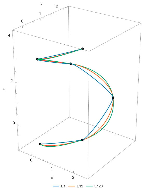
The original data are (0, 0, −1), (2, 0, 0), (2, 2, 1), (0, 2, 2), (0, 0, 3) and (2, 0, 4). Algorithm 2 is employed to carry out the constrained numerical optimization. Each objective has its own initial vertex and parameter vector. Table 1 and Table 2 report the recalculated results, and Figure 1 uses these full-precision values.

Table 1. Example 1: derivative penalties.

Method	E1	E2	E3
E1	27.5785	105.286	974.672
E12	29.129	60.1288	215.612
E123	30.8081	66.4577	80.9121
P7	31.4	76.8	0
P21	27.7404	106.396	1102.67

Table 2. Example 1: initial vertices and segment parameters.

Method	p0	α0, α1, α2, α3, α4
E1	(−1.00000000, 0.12893798, −1.50000000)	$\begin{array}{l}(0.22831857,-0.59825766,-0.75985750,\hfill \\ \hspace{1em}-0.59825766,0.22831858)\hfill \end{array}$
E12	(−1.00000000, 0.60975431, −1.50000000)	$\begin{array}{l}(0.14045646,-0.05831550,-0.19808290,\hfill \\ \hspace{1em}-0.05831550,0.14045646)\hfill \end{array}$
E123	(−1.00000000, 0.75997430, −1.50000000)	$\begin{array}{l}(0.20301512,0.15974859,0.11948619,\hfill \\ \hspace{1em}0.15974859,0.20301512)\hfill \end{array}$

Figure 1. Spatial interpolation with E1 (blue), E12 (orange), and E123 (green). Black markers are the input data. All labels are in English, and all colored curves are solid. E1 gives E₁ = 27.578465 and an interior curvature-magnitude jump of 16.566861. E123 reduces that jump to 0.189875 while increasing the first-derivative penalty. P7 has a smaller curvature jump than E123 in this example. No method dominates all reported metrics.

The maximum interpolation residual is 1.32 × 10⁻¹⁶ and the largest interior unit-tangent mismatch is 1.04 × 10⁻¹⁵. The largest projected-gradient residual of the penalty candidates is about 2.83 × 10⁻¹⁰. Varying the lower bound from −0.99 to −0.999999 leaves the E123 objective unchanged to the displayed precision; its solution is interior to these bounds.

Example 2. 

Closed planar interpolation.

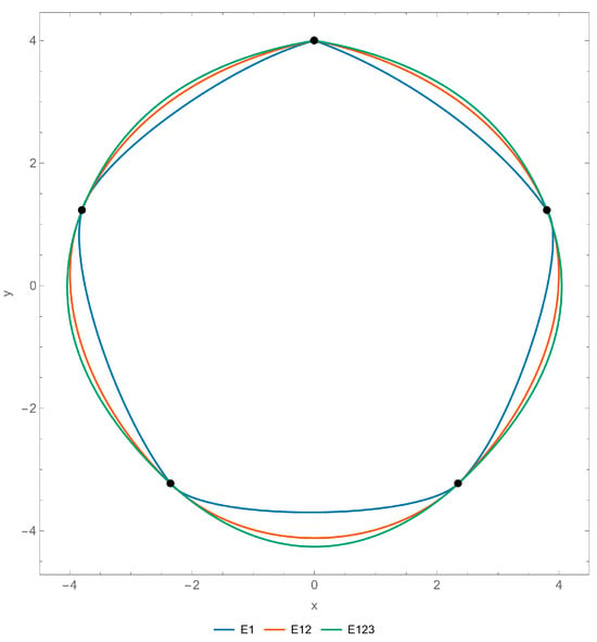
The original data are (0, 4), (3.80, 1.23), (2.35, −3.23), (−2.35, −3.23), (−3.80, 1.23) and (0, 4). Following the computational steps in Algorithm 2, all vertices are generated by recurrence at full precision. In particular, the unweighted reference p₀ = (−2.9, 4.432) gives p₁ = (2.9, 3.568) and p₂ = (4.70, −1.108). Figure 2 shows the resulting curve of this closed planar example. Table 3 and Table 4 report the derivative penalties, initial vertices and segment parameters for Example 2.

Figure 2. Planar interpolation with E1 (blue), E12 (orange), and E123 (green). Black markers are the input data.

Table 3. Example 2: derivative penalties.

Method	E1	E2	E3
E1	120.671	326.463	2709.16
E12	124.41	185.599	520.14
E123	127.482	196.31	273.51
P7	128.469	217.982	0
P21	120	327.226	3163.09

Table 4. Example 2: initial vertices and segment parameters.

Method	p0	α0, α1, α2, α3, α4
E1	(−2.50889763, 4.88956487)	$\begin{array}{l}(0.07284179,-0.41633042,-0.56132105,\hfill \\ \hspace{1em}-0.13616866,-0.21396891)\hfill \end{array}$
E12	(−2.90000000, 4.57597699)	$\begin{array}{l}(0.14315474,0.07880551,-0.05333166,\hfill \\ \hspace{1em}0.07880551,0.14315474)\hfill \end{array}$
E123	(−2.90000000, 4.47776975)	$\begin{array}{l}(0.21349520,0.19324871,0.14643600,\hfill \\ \hspace{1em}0.19324871,0.21349520)\hfill \end{array}$

The closing-seam tangent angles are 34.647945°, 22.466972° and 18.710678° for E1, E12 and E123, respectively. P21 attains a slightly smaller first-derivative penalty than E1 on these data, which rules out a general superiority claim. The maximum interpolation residual is 6.28 × 10⁻¹⁶ and the largest interior unit-tangent mismatch is 5.12 × 10⁻¹⁶. The largest penalty-candidate projected-gradient residual is about 1.18 × 10⁻⁹. Changing the lower bound from −0.99 to −0.999999 leaves the E123 objective unchanged to the displayed precision.

5. Best Approximation of the Interpolation Curve

Consider data sampled from a scalar function y = f(x) at strictly increasing abscissae. A parametric segment r_i(t) = (x_i(t), y_i(t)) defines a function graph only when its horizontal map is invertible. We impose a sufficient condition for $x_i^{\prime }(t)>0$ and measure squared vertical error with respect to the horizontal coordinate.

Definition 2. 

For increasing horizontal segments, the squared graph-approximation error is

$$\begin{array}{l}{J}_f={\displaystyle \sum _{i=0}^{n-2}{\displaystyle {\displaystyle \underset{d_{i+1,x}}{\overset{d_{i+2,x}}{\int }}}{\left[f(x)-y_i(t_i(x))\right]}^2}}\mathit{dx}\hfill \\ \hspace{1em}\hspace{1em}={\displaystyle \sum _{i=0}^{n-2}{\displaystyle {\displaystyle \underset{0}{\overset{1}{\int }}}{\left[f(x_i(t))-y_i(t)\right]}^2}}{x}_i^{\prime }(t)\mathit{dt},\hspace{1em}\hspace{1em}{t}_i=x_i^{-1}.\hfill \end{array}$$

(33)

The squared integrand prevents signed cancelation, and the horizontal derivative is the required change-of-variable factor. This is a vertical graph error, not a closest-point distance or an arc-length error. The corresponding constrained optimization problem is

$$\begin{array}{l}{\min }_{p_{0,x},p_{0,y},\alpha }\hspace{1em}{\displaystyle \sum _{i=0}^{n-2}{\displaystyle {\displaystyle \underset{0}{\overset{1}{\int }}}{\left[f(x_i(t))-y_i(t)\right]}^2}}{x}_i^{\prime }(t)\mathit{dt},\hfill \\ {\alpha }_i\in [-1+\epsilon ,1],\hspace{1em}\hspace{1em}{p}_{j+1,x}-p_{j,x}>0,\hspace{1em}j=0,\dots ,n-1,\hfill \\ p_j={(-1)}^j{p}_0+2{\displaystyle \sum _{k=1}^j{(-1)}^{j-k}}{d}_k.\hfill \end{array}$$

(34)

To justify the sufficient horizontal condition, differentiating the basis gives

$$\begin{array}{l}{x}_i^{\prime }(t)=-b_{0,2}^{\prime }(t,{\alpha }_i)(p_{i+1,x}-p_{i,x})+b_{2,2}^{\prime }(t,{\alpha }_i)(p_{i+2,x}-p_{i+1,x}),\hfill \\ -b_{0,2}^{\prime }={\displaystyle \frac{\pi }{4}}\cos {\displaystyle \frac{\mathit{\pi t}}{2}}\left(1+{\alpha }_i-2{\alpha }_i\sin {\displaystyle \frac{\mathit{\pi t}}{2}}\right)\ge 0,\hfill \\ b_{2,2}^{\prime }={\displaystyle \frac{\pi }{4}}\sin {\displaystyle \frac{\mathit{\pi t}}{2}}\left(1+{\alpha }_i-2{\alpha }_i\cos {\displaystyle \frac{\mathit{\pi t}}{2}}\right)\ge 0.\hfill \end{array}$$

(34a)

The two basis-derivative coefficients do not vanish simultaneously for admissible parameters. Strictly positive horizontal control increments therefore imply a strictly increasing horizontal map over the entire segment. The recurrence converts these inequalities into an interval for the initial horizontal coordinate. If that interval is empty, this restricted graph construction must be rejected, or another family used. Failure of this sufficient condition alone does not prove noninvertibility.

Equation (12) minimizes derivative penalties, not graph error, so it is not imposed in Equation (34). For fixed p_0,x and α, the initial vertical coordinate enters linearly. To write its elimination without suppressing the segment coefficients, set

$$\begin{array}{l}{y}_i(t)=a_i(t)p_{0,y}+y_i^0(t),\hspace{1em}\hspace{1em}{a}_i(t)={(-1)}^i(1+{\alpha }_i)\left(1-\sin {\displaystyle \frac{\mathit{\pi t}}{2}}-\cos {\displaystyle \frac{\mathit{\pi t}}{2}}\right),\hfill \\ y_i^0(t)=2(1+{\alpha }_i)\left(1-\sin {\displaystyle \frac{\mathit{\pi t}}{2}}-\cos {\displaystyle \frac{\mathit{\pi t}}{2}}\right){\displaystyle \sum _{j=1}^i{(-1)}^{i-j}}{d}_{j,y}\hfill \\ \hspace{1em}+\left[(1+{\alpha }_i)\left(\sin {\displaystyle \frac{\mathit{\pi t}}{2}}+2\cos {\displaystyle \frac{\mathit{\pi t}}{2}}-1\right)-{\alpha }_i{\cos }^2{\displaystyle \frac{\mathit{\pi t}}{2}}\right]d_{i+1,y}\hfill \\ \hspace{1em}+\left[1-(1+{\alpha }_i)\cos {\displaystyle \frac{\mathit{\pi t}}{2}}+{\alpha }_i{\cos }^2{\displaystyle \frac{\mathit{\pi t}}{2}}\right]d_{i+2,y}.\hfill \end{array}$$

(34b)

$$p_{0,y}^{*}={\displaystyle \frac{{\displaystyle \sum _{i=0}^{n-2}{\displaystyle {\displaystyle \underset{0}{\overset{1}{\int }}}{x}_i^{\prime }}}(t){(-1)}^i(1+{\alpha }_i)\left(1-\sin \frac{\mathit{\pi t}}{2}-\cos \frac{\mathit{\pi t}}{2}\right)[f(x_i(t))-y_i^0(t)]\mathit{dt}}{{\displaystyle \sum _{i=0}^{n-2}{\displaystyle {\displaystyle \underset{0}{\overset{1}{\int }}}{x}_i^{\prime }}}(t){(1+{\alpha }_i)}^2{\left(1-\sin \frac{\mathit{\pi t}}{2}-\cos \frac{\mathit{\pi t}}{2}\right)}^2\mathit{dt}}}.$$

(34c)

The denominator is positive under the stated regularized parameters and increasing horizontal map. Differentiation with respect to the vertical initial coordinate and setting the resulting linear normal equation to zero gives (34c). This eliminates only the vertical coordinate; the horizontal coordinate and parameters remain constrained optimization variables.

The numerical workflow for solving the graph-error minimization problem is outlined in Algorithm 3.

Algorithm 3. Squared graph-error approximation

Step 1. Input the function, sampled data, parameter bounds, starts and quadrature order. Derive the feasible interval for the initial horizontal coordinate from the strict control-increment conditions. Step 2. For each horizontal coordinate and parameter trial, evaluate the integrals in (34c) by 128-point Gauss–Legendre quadrature on each segment. Generate all controls by Equation (6). Step 3. Minimize the quadrature objective using analytic gradients and bound constraints from sixteen starts. Retain the best feasible candidate and record its projected-gradient residual. The reported numerical values use L-BFGS-B; the Mathematica implementation provides independent FindMinimum reoptimization. Step 4. Re-evaluate the final squared error with 512-point quadrature, verify the horizontal control increments, and report the squared error, root-mean-square error and sampled maximum absolute vertical error. Check curvature jumps independently.

Example 3. 

Interpolation and approximation of a function graph.

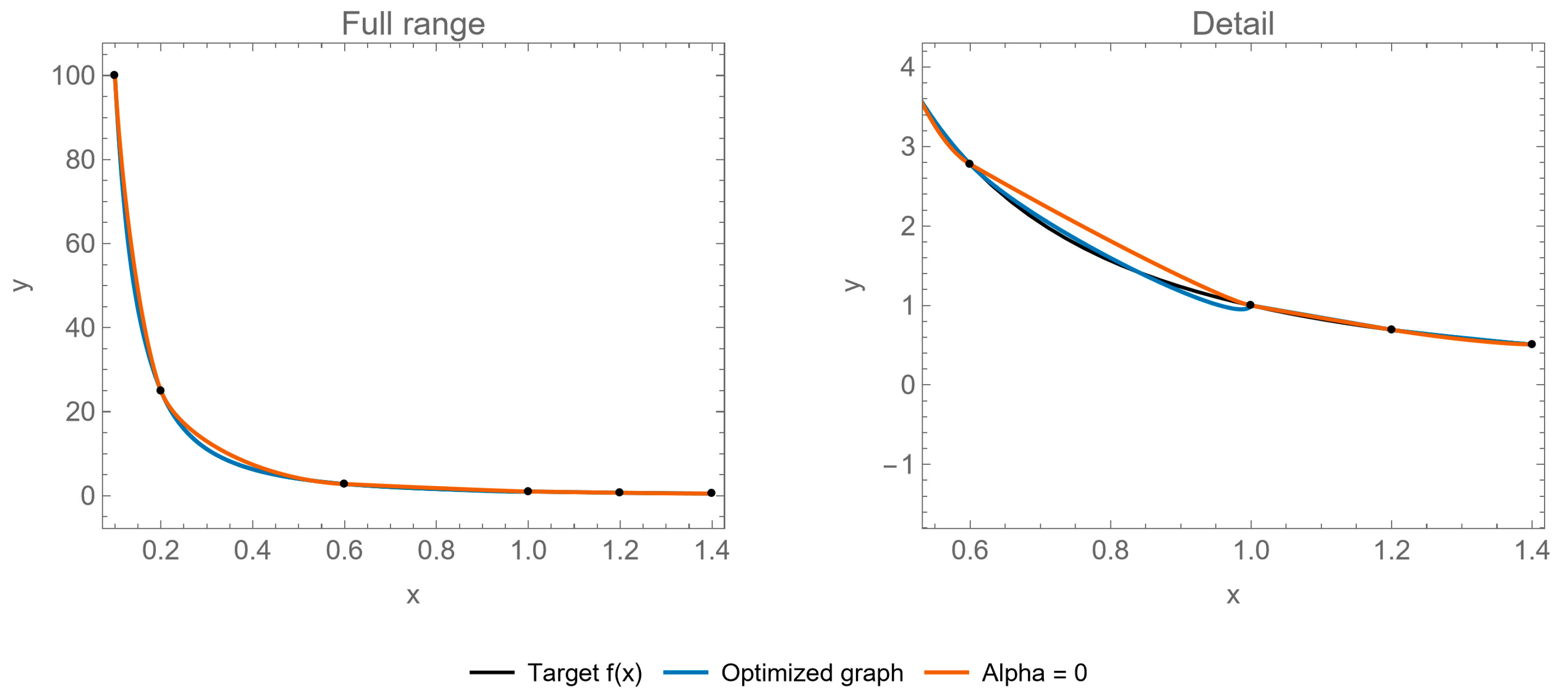
The original target is f(x) = 1/x², sampled at x = 0.1, 0.2, 0.6, 1.0, 1.2, 1.4. Function values are evaluated at full precision. We solve the graph-error minimization problem using Algorithm 3. The horizontal control condition gives 0 < p_0,x < 0.1. A margin of 10⁻⁶ times the total horizontal span gives the implemented interval [0.0000013, 0.0999987].

The recomputed initial vertex is p₀ = (0.07208547, 155.79922480), and the segment parameters are

α = (0.32083624, 0.36240396, −0.54523353, −0.99990000, −0.98448243).

(34d)

These values are rounded for display only. Figure 3 uses the supplied full-precision parameters. The smallest horizontal control increment is 0.05582906, which verifies the sufficient condition over the whole curve. Table 5 reports the actual graph errors, including $\mathrm{RMSE}=\sqrt{J_f/(1.4-0.1)}$.

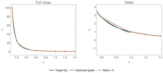
Figure 3. Graph approximation of f(x) = 1/x². The target is black, the optimized graph is blue, and the α = 0 comparator is orange. The left panel shows the full range and the right panel enlarges x ∈ [0.55, 1.4].

Table 5. Example 3: graph approximation errors.

Construction	Squared Graph Error Jf	RMSE	Sampled Maximum Error
Optimized graph	0.00530622	0.0638883	0.280094
α = 0 comparator	1.64695	1.12556	Not used for selection

The α = 0 comparator uses the same optimized horizontal initial coordinate and independently minimizes over the vertical one. It is a controlled within-family comparison, not the original method of [7] or [21]. The sampled maximum error uses 10,001 local parameter values per segment and is not a certified supremum. P7 and P21 with their original endpoint selection are not assigned graph errors because their horizontal maps are not increasing on these data.

The squared graph error is J_f = 0.0053062224. The 128- and 512-point quadrature evaluations differ by 6.33 × 10⁻¹⁷, and the projected-gradient residual is 5.82 × 10⁻¹². One parameter is at the active lower bound −0.9999. Lower bounds −0.99 and −0.999999 yield squared errors 0.005338171 and 0.005305945, respectively; these do not establish an attained optimum on the open interval (−1, 1].

The maximum interior curvature-magnitude jump is about 2.801 × 10⁷, despite the reduced squared graph error. This example therefore supports graph-error reduction but does not establish curvature fairness or monotonicity in the vertical coordinate. Such requirements need additional geometric constraints.

6. Conclusions

The midpoint constraints of the quadratic uniform trigonometric B-spline family generate all control vertices recursively from one initial vertex. For prescribed admissible parameters, complete differentiation of the first-, second-, and third-derivative penalties gives the same weighted initial vertex. The parameter-dependent weights must remain inside the sums and must be updated during parameter optimization.

The numerical examples distinguish derivative penalties from geometric measurements. They show trade-offs in length, bending energy, join regularity, and graph error; they do not guarantee general shape preservation, curvature continuity, or uniform superiority over the polynomial comparators. The graph example uses a consistent squared functional with a strictly increasing horizontal map, but it still exhibits large curvature jumps. Future work should impose explicit monotonicity, convexity, curvature, or join constraints and investigate certified global solutions where feasible.

References

- Shi, F.Z. Computer Aided Geometric Design and Non-Uniform Rational B-Splines; Higher Education Press: Beijing, China, 2013. [Google Scholar]
- Farin, G. Curves and Surfaces for CAGD: A Practical Guide; Academic Press: San Diego, CA, USA, 2002. [Google Scholar]
- Zhou, R.R.; Zhang, L.Y.; Su, X.; Zhou, L.S. Algorithmic Research on Surface Reconstruction from Dense Scattered Points. J. Softw. 2001, 12, 249–255. [Google Scholar] [CrossRef]
- Wang, Q.; Wang, R.Q.; Bao, H.J.; Peng, Q.S. A Fast Progressive Surface Reconstruction Algorithm for Unorganized Points. J. Softw. 2000, 11, 1221–1227. [Google Scholar] [CrossRef]
- Xu, Y.X.; Sui, P.X. Interpolation-quasi-interpolation form for scattered data plane. J. Zhongkai Univ. Agric. Eng. 2021, 34, 52–58. [Google Scholar] [CrossRef]
- Wu, L.J.; Guan, G.M.; Wu, J.J.; Li, L.; Han, S. Implementation of B-spline surface reconstruction algorithm based on reverse control points. J. Guangxi Univ. (Nat. Sci. Ed.) 2017, 42, 1774–1779. [Google Scholar] [CrossRef]
- Li, J.C.; Liu, C.Z.; Zhao, W.C. Planar quadratic uniform B-spline interpolation curve with optimized endpoint condition. J. Zhejiang Univ. (Sci. Ed.) 2021, 48, 159–166. [Google Scholar] [CrossRef]
- Guo, H.T.; Huang, Y.D. New extensions of quadratic uniform B-spline curve and its application. J. Hefei Univ. Technol. 2012, 35, 138–140. [Google Scholar] [CrossRef]
- Chen, L.F.; Yang, H.G.; Chen, Z.C.; Yang, J. Global path planning with integration of B-spline technique and genetic algorithm. J. Zhejiang Univ. (Eng. Sci.) 2024, 58, 2520–2530. [Google Scholar] [CrossRef]
- Wang, J.; Yang, Z.W.; Deng, J.S. Bending surfaces with algebraic tensor-product B-splines. J. Univ. Sci. Technol. China 2006, 6, 598–603. [Google Scholar] [CrossRef]
- Han, X.L. Piecewise Quadratic Trigonometric Polynomial Curves. Math. Comput. 2003, 72, 1369–1377. [Google Scholar] [CrossRef] [Scilit]
- Meng, L.J.; Wang, Z.; Liu, Y.H.; Chang, J.C. Research on Trigonometric B-Spline Functions and the Drawing of Transcendental Curves and Surfaces. J. North China Univ. Sci. Technol. (Nat. Sci. Ed.) 2025, 47, 106–115. [Google Scholar] [CrossRef]
- Munir, N.A.A.; Hadi, N.A.; Nasir, M.A.S. Constrained for G1 Cubic Trigonometric Spline Curve Interpolation. Malays. J. Fundam. Appl. Sci. 2022, 18, 323–331. [Google Scholar] [CrossRef] [Scilit]
- Wang, C.W.; Zhang, J.M. C2 Continuous Quasi-cubic Trigonometric Adjustable B-Spline Curves: Tangent to Given Polygon and Applications in Modelling. J. Beijing Inst. Cloth. Technol. (Nat. Sci. Ed.) 2020, 28, 67–71. [Google Scholar] [CrossRef]
- Lü, Y.G.; Wang, G.Z.; Yang, X.N. Uniform Trigonometric Polynomial B-Spline Curves. Sci. China Ser. E 2002, 32, 281–288. [Google Scholar] [CrossRef]
- Xu, G.; Zhu, Y.F.; Deng, L.S. Efficient construction of B-spline curves with minimal internal energy. CMC-Comput. Mater. Contin. 2019, 58, 879–892. [Google Scholar] [CrossRef] [Scilit]
- Zhang, Y.W.; Li, Y.J.; Deng, C.Y. Point-Normal Interpolatory B-Spline Curve and Surface with Minimal Energy. J. Comput.-Aided Des. Comput. Graph. 2023, 35, 1894–1899. [Google Scholar] [CrossRef] [Scilit]
- Li, J.C.; Zhang, L. Length and curvature variation energy minimizing planar cubic G1 Hermite interpolation curve. J. Taibah Univ. Sci. 2020, 14, 60–64. [Google Scholar] [CrossRef] [Scilit]
- Li, J.C.; Liu, C.Z.; Guo, X. Planar Piecewise Cubic Parametric Hermite Interpolation with Minimal Derivative Oscillation and Strain Energy. Math. Numer. Sin. 2022, 44, 97–106. [Google Scholar] [CrossRef]
- Li, J.C.; Liu, C.Z.; Hu, L.J.; Liu, S.J. Shape optimization of the planar cubic Cardinal spline curve. J. Zhejiang Univ. (Sci. Ed.) 2026. online first publishing. [Google Scholar] [CrossRef]
- Xie, J.; Chen, X.Q.; Wang, S.L.; Jia, Y.S. Control point generation and optimal interpolation for quadratic uniform B-splines with parameters. J. Shandong Univ. (Nat. Sci.) 2026, 61, 127–134. [Google Scholar] [CrossRef]
- Kaklis, P.D.; Stamatelopoulos, S.; Ginnis, A.-A.I. Shape-preserving interpolation on surfaces via variable-degree splines. Comput. Aided Geom. Des. 2024, 109, 102276. [Google Scholar] [CrossRef] [Scilit]
- Mahzir, S.S.; Misro, M.Y. Enhancing curve smoothness with whale optimization algorithm in positivity and monotonicity-preserving interpolation. AIMS Math. 2025, 10, 6910–6933. [Google Scholar] [CrossRef] [Scilit]
- Gabrielides, N.C.; Sapidis, N.S. Point-normal convexity preserving curve interpolation. Comput.-Aided Des. 2025, 180, 103836. [Google Scholar] [CrossRef] [Scilit]
Disclaimer/Publisher’s Note: The statements, opinions and data contained in all publications are solely those of the individual author(s) and contributor(s) and not of MDPI and/or the editor(s). MDPI and/or the editor(s) disclaim responsibility for any injury to people or property resulting from any ideas, methods, instructions or products referred to in the content. |
© 2026 by the authors. Licensee MDPI, Basel, Switzerland. This article is an open access article distributed under the terms and conditions of the Creative Commons Attribution (CC BY) license.