


Abstract
Learning-based routing for the Capacitated Vehicle Routing Problem with Time Windows (CVRPTW) must let a policy visit infeasible states in training, yet deploy routes that provably respect every time window under stated assumptions. In existing deep reinforcement learning (DRL) methods, however, time information serves a single constraint-handling mode, fixed for training and inference. We propose ETHC-VRC, a DRL construction method whose explicit time state is shared by the decoder context and the hard time-window mask, so that a policy trained with soft penalties can be decoded under this mask without retraining; its hybrid constraint strategy decodes each instance in both modes and keeps the lower-cost solution. On 20- to 100-node instances, greedy decoding solves 10,000 instances within seconds on a GPU at a lower hybrid cost than the greedily decoded DRL baselines (not significantly against MVMoE at 100 nodes). Sampling 1280 solutions per mode lowers it by another 3.8–4.9% at 0.07–0.32 s per instance, to within 2.1–4.3% of OR-Tools run for 10–120 s per instance and below OR-Tools at equal time. In zero-shot generalization across five scales, greedy decoding stays ahead of TPA-Reward on all 15 training–test combinations and of MVMoE, which has 5.3 times the parameters, on 8. A single model thus offers an explicit quality–latency trade-off, which we expect to suit both latency-critical and quality-critical logistics applications.
1. Introduction
Smart logistics has emerged as a critical component of modern circulation systems under China’s strategy of building a country with a strong transportation network, creating urgent demands for intelligent optimization of distribution networks to improve efficiency and reduce operating costs [1]. Driven by the sustained expansion of China’s e-commerce and express delivery sectors, the annual express parcel volume reached 174.5 billion in 2024, while an increasingly extensive urban–rural distribution network provided a strong operational foundation for the large-scale deployment of smart logistics [2,3]. As this operational scale continues to expand, the industry urgently requires routing solutions capable of simultaneously handling complex constraints such as vehicle capacity limits and customer time-window requirements [4], while achieving near-optimal solution quality with real-time response capabilities to support dynamic decision-making in large-scale distribution networks [5,6]. Advances in operations research and machine learning have established a broad algorithmic foundation for vehicle routing [7], with exact solvers [8,9], metaheuristics [10], and emerging neural combinatorial optimization methods [11] collectively providing growing technical capabilities for tackling such multi-constrained routing tasks. However, traditional exact algorithms suffer from prohibitive computational costs when handling such multi-constrained large-scale instances, while heuristic algorithms, though fast, struggle to guarantee solution quality [12]. This compelling demand for methods that simultaneously achieve solution quality and computational efficiency has driven growing research interest in learning-based approaches, motivating the development of neural construction methods that learn high-quality routing policies through end-to-end training [13]. Applying Deep Reinforcement Learning (DRL) to solve constrained vehicle routing problems has thus become a vital research direction, aiming to develop neural network-based construction methods that learn high-quality decision-making policies through end-to-end training while maintaining fast inference speed [14,15,16].
While some DRL-based studies have considered VRP variants with capacity constraints [17,18], these constraints are relatively simple and are typically handled through straightforward hard masking rules during action selection. Recently, DRL-based approaches have begun to explore VRPTW variants. Efficient multi-vehicle route generation has been addressed using a multi-agent attention model [19], while time-window constraints have been handled by combining masked algorithms with pointer networks [20]. When handling problems with both capacity and time-window constraints, existing approaches rely on hard masking to enforce feasibility at every step, on soft constraints with penalty terms that allow constraint violations during training, or on a combination of the two [21,22]. However, these methods either increase system complexity through multi-agent frameworks or do not examine the contribution of the temporal state to solution quality separately from that of masking or reward design [21,23]. Furthermore, existing methods bind the two phases to the same constraint handling: purely soft-constraint approaches maintain training flexibility but cannot certify feasibility, hard-masking methods enforce feasibility at every step but also remove infeasible actions from exploration during learning, and methods that combine penalties with masking apply the same combination in both phases. The two requirements are treated as one knob that must be set once, for both phases [22,24]. These deficiencies result in optimization methods that struggle to achieve high solution quality, fast inference speed, and strong generalization capability concurrently, limiting their practical deployment in real-world logistics scenarios. Based on the above limitations, this paper investigates how to develop a DRL-based solution for CVRPTW that addresses two core challenges: designing an explicit time-state architecture that natively integrates temporal information for jointly modeling capacity and time-window constraints, and establishing a hybrid constraint-handling strategy that separates training-phase flexibility from inference-phase feasibility guarantees.
This paper aims to construct a time-window-aware architecture with dynamic constraint handling mechanisms for jointly modeling capacity and time-window constraints in CVRPTW, and establish a penalty-guided training framework that balances solution feasibility and quality. To this end, this paper develops an improved Transformer-based approach that incorporates architectural design for temporal constraint modeling, proposes constraint-handling mechanisms for balancing training and deployment requirements, and conducts systematic experimental validation across diverse problem scales. Based on the above innovations, the main contributions of this paper include the following:
- we propose an explicit time-state representation whose variables and update rule are shared by the decoder context, the hybrid cost and the hard time-window mask, so that one policy trained under soft constraints perceives time during training and can be decoded under the hard mask at deployment without retraining.
- we propose a hybrid constraint strategy that trains with penalty-based soft constraints and, at inference, mixes soft-constrained and hard-masked decoding and keeps the lower-cost solution for each instance, so that the same trained model yields exploratory training dynamics, competitive deployed solutions, and, under the assumptions of Section 4.3.2, a strictly feasible alternative when required. Building upon penalty-guided approaches in recent work, this design allows complete solution feasibility to be enforced in safety-critical scenarios by deploying the hard-masked solution, which is feasible under the assumptions of Section 4.3.2, while maintaining training flexibility through the penalty term.
- we evaluate zero-shot generalization across five problem scales, where greedy decoding stays ahead of TPA-Reward on all 15 combinations of training and test size and ahead of MVMoE, which has 5.3 times as many parameters as ETHC-VRC, on eight of them, and sampling lowers the hybrid cost further on every combination. Through a comparison of greedy and sampling-based decoding and an analysis of the cost distribution of sampled solutions, we characterize the trade-off between solution quality and inference time offered by the two decoding modes of a single trained model.
2. Related Works
Classical and learning-based methods for vehicle routing can be grouped into metaheuristics, iterative improvement methods, hybrid strategies that combine learning with search, and constructive neural policies.
We review each group with respect to time windows and point out its methodological limitations.
2.1. Metaheuristics
Metaheuristics remain the reference methods for the VRPTW [25,26].
Local search methods such as tabu search [27] and variable neighborhood search [10] intensify the search around incumbent solutions, whereas population-based methods such as genetic and swarm algorithms, including the Bees Algorithm [28], explore the search space more broadly at a higher computational cost [12].
Their solution quality depends on three factors: how widely the search space is explored, how the parameters, e.g., the population size, the neighborhood structures or the tabu tenure, are set, and how much computation is allowed; with a short time limit, their quality can drop sharply.
The same trade-off between search budget and solution quality arises in other discrete selection problems: in selected-mapping (SLM) peak-to-average power ratio reduction for optical OFDM systems, the best of several candidate signals is selected, and discrete forest optimization [29] and migrating birds optimization [30] search the phase factors with fewer evaluations, and hence a lower computational complexity, than conventional SLM, with results that depend on the algorithm’s parameters.
The time limits and parameters of our metaheuristic baselines, and the number of solutions sampled by ETHC-VRC, face the same trade-off.
In our experiments, OR-Tools with guided local search [31], tabu search and the Bees Algorithm represent these classes and serve as quality references under the time limits given in Section 5.
2.2. Iterative Improvement and Hybrid Methods
Improvement methods start from a complete solution and learn which local modification to apply next.
Wu et al. [18] proposed self-attention-based improvement heuristics with strong generalization across problem sizes, and Ma et al. [32] proposed flexible neural k-opt, which searches both feasible and infeasible regions of routing problems and thereby explores the constraint boundary.
Hybrid methods embed learned components in a classical search, such as neural large neighborhood search [17].
These methods usually reach better solutions than a single constructive pass, but they need many iterations per instance at inference, so their runtime grows with the search budget, and most of them were developed for capacity constraints rather than time windows.
2.3. Constructive Neural Policies
Constructive neural policies build a solution node by node with a learned policy, usually trained by reinforcement learning, and have shown strong generalization and computational efficiency on vehicle routing problems [33]. Vinyals et al. [34] introduced Pointer Networks using sequence-to-sequence attention for the TSP, Kool et al. [35] advanced the field with Transformer-based attention models that achieved near-optimal results on several VRP variants, and POMO [36] improved such policies with multiple rollouts from symmetric starts; attention-based policies have also been extended to heterogeneous fleets and relational structures [37,38]. For time windows, Wang et al. [20] employed masked pointer networks, Zhang et al. [19] developed a multi-agent attention model with soft time windows, Lin et al. [39] addressed electric vehicles with charging and time-window constraints, Zhang et al. [21] proposed a manager-worker framework for multiple TSP with time windows and rejections, in which a Graph Isomorphism Network-based manager assigns customers to vehicles, Zong et al. [24] augmented the reward with time penalties for multi-vehicle VRPTW (TPA-Reward), and Zhou et al. [23] introduced MVMoE, a mixture-of-experts solver for ten VRP variants including VRPTW.
Constructive policies build a solution with one forward pass per decision and are therefore fast, but they have two limitations for time-windowed problems.First, a single greedy rollout leaves a gap to the best known solutions, which is usually narrowed by sampling many solutions per instance at a cost that grows with the number of samples.Second, their handling of time windows is fixed at training time and applied unchanged at deployment: MVMoE [23] and PolyNet [40] mask infeasible actions during both training and inference, which keeps every step feasible but removes infeasible actions from exploration; penalty-based designs [19,24] keep training flexible but cannot certify feasibility at deployment, and reported violation rates vary widely across settings; and Bi et al. [22] combine penalties with proactive infeasibility masking for TSPTW and TSPDL, again, identically in both phases. How temporal information enters the policy also differs: MVMoE supplies the current time to its decoder, the manager of Zhang et al. [21] keeps the temporal state inside its hidden representation, and TPA-Reward exposes time only through the reward.
Research gap.
Constraint-aware neural methods, whether constructive, iterative or hybrid, handle time windows in the same way during training and deployment: soft constraints keep training flexible but cannot guarantee feasibility, while hard constraints enforce feasibility at every step but remove infeasible actions from exploration, and because the constraint mode is fixed once, this trade-off has to be settled for both phases together.
What is missing is a constructive policy whose constraint handling is decoupled between the two phases, trained with the flexibility of penalties and deployed with the guarantee of a mask, without retraining.
ETHC-VRC builds on the attention model of Kool et al. [35]: its encoder is a Transformer encoder, and its decoder adds the explicit time-state context of Equation (11). What distinguishes it from existing methods is how this decoder handles time windows.Unlike the time-aware DRL methods above [22,23,24], whose constraint-handling scheme cannot be changed without retraining, so that all their solutions are decoded under one constraint mode, ETHC-VRC differs in three respects: it trains one policy under soft constraints only; it decodes this policy under both a soft and a hard mask, with a greedy or a sampling budget and without retraining; and it keeps the better of the two solutions for each instance, the hard-masked one being feasible under the assumptions of Section 4.3.2. This is made possible by the explicit time state, which serves both as decoder context and to define the hard mask and also determines the lateness in the hybrid cost, so that a policy trained with soft penalties can be deployed under either constraint mode without retraining.
3. Problem Description
3.1. Problem Background
In CVRPTW, a fleet of vehicles services customers spread across different locations, each with a specific service time window. Vehicles start from a central depot, visit assigned customers within their capacity limits, and return to the depot. If a customer is not serviced within the specified time window, this leads to dissatisfaction and incurs penalties. The optimization challenge lies in balancing route efficiency (minimizing travel distance) with temporal constraint satisfaction (respecting time windows). Before presenting the mathematical formulation, we define the key concepts involved in CVRPTW:
- Customer: A service point with a specific location, demand, and time-window constraint that needs to be visited by a vehicle.
- Depot: The starting and ending point of all vehicle routes, where vehicles begin their journeys and return after completing their routes.
- Time Window: A time interval during which a customer must be serviced. Early arrival requires waiting, while late arrival incurs penalties.
- Subtour: A route traveled by a single vehicle, starting from the depot, visiting a sequence of customers, and returning to the depot.
- Hybrid Cost: A weighted combination of route length and time-window violation, used to balance solution quality and constraint satisfaction.
3.2. Notation
Table 1 summarizes the notations used in formulating the CVRPTW problem, including problem parameters, decision variables, and cost-function components.
Table 1.
Notations for CVRPTW problem formulation (times in hours).
3.3. Problem Formulation
3.3.1. Problem Instance
A CVRPTW instance consists of a depot and n customers, denoted as . Each customer has a 2D position , a demand , and a time window where . The depot is represented as with no demand or time constraint. Homogeneous vehicles with capacity C are available to service all customers; unlike formulations that fix the fleet size or, as in the Solomon benchmark, minimize it first, the fleet size m is determined by the constructed solution, since a new route starts each time the vehicle returns to the depot, and the objective contains no fixed cost per vehicle. Surplus vehicles are still discouraged, because merging two routes never increases the total length when capacity and time windows permit.
3.3.2. Decision Variables
The decision variables define a complete solution , where each represents the route for vehicle j. Each route is an ordered sequence starting from the depot, visiting customers, and returning to the depot. The variables to be determined are as follows: (1) customer assignment - which customers are assigned to which vehicle; (2) visit sequence - the order in which each vehicle visits its assigned customers.
3.3.3. Objective Function
The objective is to minimize the total hybrid cost , which balances route efficiency and time-window compliance:
where the hybrid cost for route consists of the following:
Route Length
The total travel distance of vehicle j:
where is the Euclidean distance between consecutive customers.
Time-Window Violation
The total time violation penalty for route :
where is the arrival time at customer , i.e., the value of the state variable when is reached, and measures the lateness.
Penalty Coefficient
The parameter controls the trade-off between route length and time-window compliance. Using a hybrid cost reduces ambiguity in solution quality: focusing solely on time violations could produce routes with vastly different lengths, while the hybrid formulation enables selecting shorter routes that maintain acceptable time compliance.
3.3.4. Constraints
The feasible solution space is defined by the following constraints:
Customer Coverage
Each customer must be visited exactly once:
Vehicle Capacity
The total demand on each route cannot exceed vehicle capacity:
Depot Constraint
All routes must start and end at the depot:
Time-Window Handling
If a vehicle arrives before , it waits until the time window opens; arrival after incurs penalty in the objective function, enabling soft constraint handling that balances exploration during training with feasibility requirements during deployment.
4. Proposed Method
4.1. Method Framework
This study proposes a deep reinforcement learning framework that integrates an improved Transformer architecture for solving CVRPTW, as illustrated in Figure 1. The framework consists of three core components: (1) a self-attention-based encoder that extracts node embeddings from customer features; (2) an explicit time-state decoder that performs sequential node selection while maintaining explicit time-state variables; and (3) a hybrid constraint-handling mechanism that balances training flexibility with deployment feasibility.
Figure 1.
Route construction process based on deep reinforcement learning framework with improved Transformer.
The input to our model is a CVRPTW instance where each customer contains position, demand, and time-window information. The output is a complete solution representing vehicle routes that satisfy the capacity constraint and minimize the hybrid cost, in which time-window violations are penalized; when the hard-masked solution is deployed, the time-window constraints are also satisfied under the assumptions of Section 4.3.2.
The Transformer architecture [41] is particularly suited for routing problems due to its self-attention mechanism that efficiently captures relationships between any pair of nodes in parallel, overcoming the sequential processing limitations of RNN-based approaches. We adopt the policy gradient method because it directly optimizes the routing policy in an end-to-end manner, learning to balance exploration and exploitation during training while maintaining fast inference speed during deployment.
The routing process is formulated as a Markov Decision Process (MDP) where the policy network parameterized by defines a conditional probability distribution over actions (node selections) given the current state. Starting from the initial state , in which no customer has been visited, the policy sequentially constructs routes until reaching a terminal state where all customers are visited. Each state contains the current node, the set of visited customers, the remaining capacity and the time-state variables of Section 4, and the transition is deterministic, so a complete solution Y corresponds to exactly one action sequence . The probability of a complete solution, i.e., of its trajectory, is therefore the product of the policy probabilities along it:
In Figure 1, the step index i corresponds to t: is the state , is the node selected by the action , and is the reward of that step, i.e., the negative of the resulting increase in the hybrid cost, so that the rewards of a solution sum to .
The route construction process follows a sequential decision-making paradigm with four main steps:
- 1.
- Node Embedding: The encoder transforms customer features into -dimensional embeddings through self-attention layers.
- 2.
- Action Probability: The decoder computes selection probabilities for unvisited nodes based on current state and node embeddings.
- 3.
- Node Selection: A node is selected via greedy or sampling strategy, and the vehicle state (position, capacity, time) is updated.
- 4.
- Route Construction: Steps 2–3 repeat until all customers are visited, forming complete vehicle routes .
4.2. Explicit Time-State Encoder–Decoder Architecture
The policy network adopts an encoder–decoder architecture where the encoder extracts spatial node embeddings via self-attention, and the decoder performs sequential node selection through our proposed explicit time-state mechanism. As shown in Figure 2, the encoder leverages multi-head self-attention to capture spatial relationships between nodes, while the decoder integrates explicit time-state variables for constraint-aware action selection. The decoder’s explicit time state is the interface between the policy and the constraint handling: it enters the decoder context and defines the hard mask, and the ablation study isolates the contribution of its first role, the time-state input to the decoder.
Figure 2.
Structure of policy network for CVRPTW based on encoder–decoder architecture of improved Transformer.
4.2.1. Encoder: Self-Attention for Node Embedding
We adopt the standard Transformer encoder architecture [41] for node embedding extraction. This design choice is deliberate: the self-attention mechanism has proven highly effective for capturing spatial relationships in routing problems [35,36], enabling parallel processing of all nodes while learning long-range dependencies. Since the primary challenge in CVRPTW lies in sequential temporal reasoning during decoding rather than spatial feature extraction, we focus our architectural innovations on the decoder, while leveraging the well-established encoder design.
The encoder transforms the raw node features into -dimensional embeddings through multi-layer self-attention, where is the depot embedding. Each customer feature vector undergoes a linear projection , , and the depot, whose demand and time window are constant, is projected from its coordinates alone, ; and map the raw features to the -dimensional space. The projected embeddings are then transformed into query, key, and value vectors via learnable projection matrices for each attention head h, where and H is the number of heads. Attention scores are computed via scaled dot-product attention and aggregated across heads:
The multi-head attention output undergoes skip-connections and batch normalization [42,43]:
where FF is a two-layer feed-forward network with ReLU activation, and is the final node embedding.
In Figure 2, the block labeled GIN denotes this encoder as a whole: Equations (8)–(10) are applied in three layers, each taking the output of the previous layer in place of . Each layer follows the update of a graph isomorphism network (GIN) [44]: the aggregate of the node embeddings is added to each node’s own embedding, and the result is passed through a feed-forward network (Equation (10)). Unlike the original GIN, which sums over graph neighbors, the aggregation is the multi-head attention of Equations (8) and (9) over all nodes of the fully connected graph, so each layer remains the Transformer encoder layer described above. The outputs are the node embeddings in Figure 2; the green block shows the per-head projections , and of Equation (8), drawn as , and is the mean embedding used in Equation (11).
4.2.2. Explicit Time-State Decoder
This section presents the explicit time-state decoder, which maintains temporal information as explicit state variables. Building on prior DRL-based routing methods [23,24], we integrate temporal dynamics directly into the decoder’s state representation and attention mechanism, and make the temporal variables and their update rule explicit so that their effect can be examined in isolation. Time-aware decoders already exist: MVMoE [23], for instance, feeds the current time to its decoder under a hard mask fixed for training and inference, and TPA-Reward [24] penalizes lateness in the reward without giving its decoder access to time. In ETHC-VRC, the same explicit state variables and , maintained by the explicit time-state update rule, enter the decoder context (Equation (11)), determine the lateness in the hybrid cost (Equation (3)) and define the hard mask (Equation (19)); a policy trained under the soft mode therefore perceives time and can be decoded under the hard mask without retraining. The decoder thus reads the current arrival time and vehicle speed when computing action probabilities, and the same variables define the hard mask of Section 4. The explicit time-state decoder consists of four key components: (1) explicit time-state representation, (2) time-state context construction, (3) masked attention for node probability computation, and (4) time-state update mechanism. The explicit time state has two parts: the state variables and their update rule, which the hard mask and the hybrid cost read, and their input to the decoder context (Equation (11)). Switching between the masking modes relies on the first part only.
Explicit Time-State Representation
Beyond the positional and capacity information maintained by standard attention-based decoders for CVRP, our decoder explicitly tracks temporal variables as state components. At each decision step t, the state maintains the following variables:
- : Arrival times at the present nodes of the batch (hours)
- : Vehicle traveling speeds (coordinate units per hour, identical for all vehicles)
- : Remaining vehicle capacities
- : Embeddings of the current nodes
- : Mean embedding of all nodes
Since decoding is carried out in parallel for a mini-batch of instances, the explicit state variables , and are vectors in , written in upper case to distinguish them from the learned embeddings and ; when an operation is described for a single instance, as in the update procedure and Equations (18) and (19), the same symbols denote that instance’s entries.
Attention-based decoders for CVRP maintain only positional and capacity information; time-windowed variants either supply the elapsed time to the decoder, as MVMoE does, or leave it to be inferred from the action sequence, as TPA-Reward does. In our decoder, the time state is supplied explicitly and is the same state from which the hard mask is computed.
Checking the time window of a candidate from the maintained arrival time takes constant time; what matters here is that the check reads the same state that the policy sees during training and that defines the lateness in the hybrid cost, so the hard mask (Equation (19)) can be applied at inference to a policy trained without it, and every hard-masked solution is feasible under the assumptions of Section 4.3.2. This provides a more transparent and reliable mechanism for constraint handling.
The explicit time-state enriches the decoder’s context when computing attention scores, allowing the model to learn temporal-spatial correlations between nodes. For instance, the attention mechanism can directly reason about whether visiting a distant customer is feasible given the current arrival time and remaining time windows, rather than indirectly inferring temporal constraints from node sequences.
Time-State Context Construction
The decoder constructs a time-state context vector that integrates spatial, capacity, and temporal information. Beyond the node embeddings and remaining capacity used by standard attention decoders for CVRP, our context explicitly incorporates time-state variables:
where is the query vector augmented with time-state, projects the concatenated state to match embedding dimensions, and is the multi-head attention glimpse that captures global context, which, like Equation (14), attends only to the nodes selectable under the active masking mode. The learnable parameters enable the model to learn which temporal patterns are most relevant for action selection. In Figure 2, is the query of Equation (11): the ⊕ is the sum in that equation, the entering it is the embedding of the current node, which is the depot at the first step, and its concatenation with , and is not drawn; , and of the first decoder block are the per-head matrices , and of Equation (12).
Masked Attention for Node Probability
Given the time-state context, the decoder computes selection probabilities via masked attention:
where is the set of selectable nodes under the active masking mode, i.e., or in Equations (18) and (19), is the embedding dimension, and compresses scores to for exploration [45]. Nodes outside are masked with to ensure zero selection probability. The second decoder block of Figure 2 () corresponds to and of Equation (13); the node probabilities are computed with a single head, and both decoder blocks use the selectable set of the active masking mode.
Time-State Update
After selecting node , the state is updated to reflect the vehicle’s new position, capacity, and arrival time, as summarized in Algorithm 1.
| Algorithm 1 Explicit Time-State Update |
|
The algorithm explicitly tracks the arrival time and handles time-window constraints: if the vehicle arrives before the customer’s earliest service time , it waits; otherwise, it records the actual arrival time (which may violate the latest time , incurring penalties in the hybrid cost function). When the depot is selected, the remaining capacity is restored to C and the time is reset to zero, so that each route is performed by a different vehicle departing from the depot at time zero; the m routes of a solution therefore represent m vehicles working in parallel rather than one vehicle serving several trips. This explicit time-state maintenance provides a clear and direct mechanism for feasibility checking at each decision step, which is activated as a hard mask in the hard-masked decoding pass at inference.
4.3. Hybrid Constraint-Handling Strategy
We propose a hybrid constraint-handling strategy that trains the model under soft constraints for exploration flexibility and, at inference, combines soft-constrained and hard-masked decoding so that the better of the two solutions is deployed. During training, we employ penalty-based soft constraints that allow time-window violations at a cost, to enable policy exploration. During inference, each instance is decoded once under the soft mode and once with hard masking, and the solution with the lower hybrid cost is retained; when strict feasibility is required, as in safety-critical applications, the hard-masked solution can optionally be deployed on its own.
Existing DRL-based routing methods typically adopt purely soft constraints (which maintain training flexibility but cannot guarantee feasibility), uniform hard constraints (which enforce feasibility at every step but also remove infeasible actions from exploration during learning), or a fixed combination of the two, applying the same handling to both phases in every case. Our hybrid strategy overcomes this dilemma by training under the soft mode only and mixing both modes at inference: because the time-window term of the mask (Equation (19)) can be switched on without retraining, a single set of weights yields both a soft-constrained and a hard-masked solution for every instance, and the one with the lower hybrid cost is kept.
We train under soft constraints so that the policy may visit near-feasible states and learn from the penalized cost of lateness instead of having these actions removed by the mask. This is a design motivation: we do not compare soft training with hard-masked training of the same architecture, and our contribution lies in decoupling the constraint handling of training and inference rather than in the training mode itself.
In the hard-masked decoding pass, masking eliminates all infeasible actions by setting their selection probabilities to zero. Deploying the hard-masked solution alone therefore guarantees that all constraints are satisfied under the assumptions of Section 4.3.2, which is essential for safety-critical scenarios such as medical supply delivery or time-sensitive logistics operations where constraint violations are unacceptable. Otherwise, keeping the lower-cost of the two solutions means that the deployed hybrid cost is never higher than that of either mode alone, while the hard-masked solution remains available as a feasible alternative.
The hybrid strategy is implemented through three components:
4.3.1. Soft Constraint with Penalty Coefficient
During training, we minimize a hybrid cost function that combines route length and time-window violations:
where is the total route length, is the total time-window violation (sum of lateness across all customers in route j), and is the penalty coefficient.
Penalty coefficient: We parameterize the penalty coefficient as
where is a dimensionless penalty scaling factor and coordinate units per hour is a reference rate that converts lateness, measured in hours, into the unit of route length, so that in Equation (1) is a length. Numerically, equals the working horizon of our instances, but it is a fixed constant rather than a rule that scales with the instance; a larger increases the penalty imposed for time-window violations. Since the vehicle travels coordinate units per hour, one hour of lateness costs as much as hours of extra travel, i.e., 12 h at the default . Section 5.2.2 examines how the results vary with .
4.3.2. Soft and Hard Masking Modes
The decoder supports two masking modes that differ only in whether the time-window condition is enforced. The set of selectable nodes at step t is defined for the soft mode and the hard mode, respectively, as
Both selectable sets also contain the depot, except when the vehicle is already there and some customer is selectable; nodes outside the selectable set of the active mode are masked with in equation (14), ensuring zero selection probability; in the hard mode, this excludes every node that would violate capacity, visitation or time-window constraints. The assumptions under which this local rule always completes a feasible solution are stated below. Training uses the soft mode only, so that the policy may explore near-feasible regions under the penalty term. At inference, each instance is decoded under both modes and the solution with the lower hybrid cost (Equation (1)) is retained; this combination of the two modes is what we refer to as hybrid constraint handling.
Feasibility of hard-masked decoding.
Although the hard mask checks only the next node, decoding in the hard mode (Equation (19)) always terminates with a solution that visits every customer exactly once and satisfies all capacity and time-window constraints, provided that (i) the number of vehicles is not limited; (ii) for every customer i; (iii) every customer can be reached on time directly from the depot, i.e., ; (iv) every route leaves the depot at time 0 with capacity C; (v) the depot has no closing time and service times are zero; and (vi) a vehicle that arrives early waits until .
By Equation (19), a customer can be selected only if it is unvisited, its demand fits the remaining capacity and the vehicle reaches it no later than ; with waiting (vi) and zero service times (v), the arrival time after the move is , so every selected customer is served within capacity and on time. Returning to the depot is always allowed, since the depot has no closing time (v). At the depot, a new route starts at time 0 with capacity C (iv), and by (ii) and (iii), every unvisited customer is then selectable, so the depot is never selected twice in a row while customers remain. Each route therefore serves at least one new customer, and after at most n routes, which are available by (i), every customer has been served.
All instances in this study satisfy these assumptions: the depot and the customers lie in the unit square, so h, whereas every time window closes at least 2 h after the start of the day, and demands are at most 9, below the smallest capacity of 30. The hard-masked solutions are therefore feasible by construction, in agreement with the experiments, in which all of them satisfy every time window.
These assumptions describe our experimental setting, in which the number of vehicles is effectively unrestricted (Section 3), and they do not hold for the general CVRPTW. With a fixed fleet, deciding whether a feasible solution exists is itself NP-complete [46], so no rule that checks only the next node can guarantee completion; and with a depot closing time or nonzero service times, the mask would also have to check that the vehicle can still return to the depot in time, which Equation (19) does not do.
We implement two decoding strategies:
- Greedy: Select the highest-probability feasible node at each step:
- Sampling: Sample from the probability distribution over feasible nodes:
Under the hybrid constraint strategy, both decoding strategies are applied in each masking mode: greedy decoding yields one soft-constrained and one hard-masked solution per instance, sampling draws 1280 solutions in each mode, and the solution with the lowest hybrid cost is retained. Sampling also provides a diverse set of candidate solutions.
4.3.3. REINFORCE Training with Rollout Baseline
We train the policy network using the REINFORCE algorithm [47] with a rollout baseline to reduce gradient variance. For a problem instance X with initial state , the policy gradient is
where is the baseline cost obtained by greedily rolling out a frozen policy .
The baseline policy is updated periodically: at the end of each epoch, we evaluate both the current policy and baseline policy on a validation set. If a paired t-test (significance level ) shows statistically significant improvement, we update . This strategy, similar to target network freezing in DQN [48], stabilizes training.
Algorithm 2 summarizes the complete training procedure, which realizes the training-phase (soft-constraint) part of the hybrid strategy within policy-gradient optimization; the inference-phase combination of the two masking modes is described at the end of this section.
| Algorithm 2 Training of ETHC-VRC with Soft Time-Window Constraints |
|
The training procedure emphasizes three key aspects: (1) Time-State Initialization (line 5): Each state explicitly maintains temporal variables (, ) alongside traditional routing state; (2) Soft constraint training (lines 6–8): During rollouts, the policy explores near-feasible regions by allowing time-window violations, which are penalized through the hybrid cost function; (3) Baseline stabilization (lines 12–14): Statistical testing ensures that baseline updates occur only when genuine improvement is achieved, preventing training instability.
During inference (not shown in the training algorithm), each instance is additionally decoded with hard masking, i.e., with infeasible nodes’ probabilities set to in Equation (14), and the lower-cost of the soft-constrained and hard-masked solutions is retained; for deployment scenarios that require strict feasibility, the hard-masked solution can optionally be used on its own, guaranteeing constraint satisfaction under the assumptions of Section 4.3.2.
5. Experiments and Results
In this section, the effectiveness of our method is evaluated through extensive experiments. First, we compare our method with the state-of-the-art DRL methods and three advanced metaheuristic methods. Problem instance sizes vary between 20 and 100 nodes to examine scalability across the instance sizes considered here. In addition, this paper provides a detailed evaluation of the greedy and sampling strategy used in our method. Subsequently, we conduct several detailed analytical studies. To facilitate further research and reproducibility, the implementation of the proposed method and of all baselines, the instance generator with its seeds, the trained models and the scripts that reproduce every table and figure of this paper are publicly available on our GitHub (https://github.com/yeqing9349/ETHC-VRC, accessed on 25 October 2026) repository; the version used for this paper is tagged paper-r2, and the repository also documents the implementation details and hyperparameters not listed in the paper.
5.1. Experimental Setup
5.1.1. Dataset and Metrics
Following standard DRL benchmarks for routing problems [34,35,49,50], we generated synthetic instances with sizes delivery nodes (excluding depot) and corresponding vehicle capacities . Each instance consists of the depot and delivery node locations , demands , and time windows derived from an eight-hour workday divided into four periods: with duration 0.25 in units of h, i.e., and h. Vehicles travel at coordinate units per hour, so the travel time between two nodes is hours, and service times are zero. For each size, 1,280,000 training instances were generated anew in every epoch (batch size 512 across 2500 iterations per epoch), and 10,000 instances each were used for validation and testing, ensuring no overlap between sets to prevent data leakage.
We adopted three standard metrics to comprehensively evaluate method performance [21,35]: (1) Hybrid cost, the objective of Equation (1), combining total route length (the sum of Euclidean distances traveled by all vehicles) and the total time-window violation weighted by , serving as the primary optimization objective; (2) Gap, the percentage difference from the best solution reported in Table 2, which is not a proven optimum; and (3) Computational time, the wall-clock time required to solve the entire 10,000-instance test set, evaluating real-time scalability. For the solution output by each method, Table 2 also reports the route length, the feasibility rate (percentage of instances without time window violations), the average lateness of a late customer in minutes and the average number of vehicles. Under the hybrid constraint strategy, ETHC-VRC(G) decodes each instance greedily once under the soft mode and once with hard masking, and ETHC-VRC(S) draws 1280 samples under each of the two modes; in both cases, the solution with the lowest hybrid cost is reported. For ETHC-VRC(G), instances are processed in batches of 1024 and the reported time is the total over the whole test set, so the time per instance is an amortized value; for ETHC-VRC(S), the 1280 samples of an instance in each mode are drawn in a single batched forward pass and the instances are decoded one after another, so the reported total divided by 10,000 is the latency of a single instance. In both cases, the reported time includes both the soft-constrained and the hard-masked decoding passes. These metrics assess solution quality, with time-window violations entering through the penalty term of the hybrid cost, and computational efficiency; two methods evaluated on the same test instances are compared through their per-instance differences in hybrid cost, reporting the mean difference, relative to the mean cost of the second method, with its 95% confidence interval from the paired t-distribution, and the p-value of a two-sided Wilcoxon signed-rank test.
Table 2.
Performance comparison of our method (ETHC-VRC) with baseline methods on CVRPTW with 20, 50 and 100 nodes (10,000 test instances per size, ). Obj.: hybrid cost (Equation (1)); for ETHC-VRC, it is the cost of the solution selected per instance from the soft-constrained and hard-masked decoding passes. Gap: relative to the best Obj. at the same size, not to a proven optimum. Length: route length. Feas.: share of instances without time-window violations. Late: average lateness of a late customer in minutes (–: no late customer). Veh.: average number of vehicles. Time: total wall-clock time for the whole test set, including both decoding passes for ETHC-VRC. (G) denotes greedy decoding and (S) sampling with 2560 candidates per instance: ETHC-VRC decodes under both constraint modes (one greedy pass or 1280 samples in each mode), TPA-Reward under the soft mode and MVMoE under the hard mode (one greedy pass or 2560 samples), so that all (S) rows use the same number of candidates. OR-Tools, TS and BA use the same penalty coefficient as the DRL methods, a fleet of 12 vehicles and the time limits given in Section 5; they run on the CPU with parallel worker processes, so their times are given for reference only. The best results are highlighted in bold.
5.1.2. Baseline Methods
To ensure fair comparison and reproducibility, all methods were evaluated on identical test instances, and TPA-Reward was retrained on instances drawn from the same generator with the same penalty coefficient as our method; MVMoE was likewise retrained on instances from the same generator, on CVRPTW alone rather than on its original multi-task mix. All models were trained, and all methods evaluated, with the publicly released code: TPA-Reward was re-implemented following the architecture of its original paper (a pointer decoder that orders the customers and a parameter-free task handler that assigns them to vehicles), and MVMoE was ported from its official implementation. The policy network architecture consisted of 3 attention layers with 8 heads and embedding dimension 128. Training employed Adam optimizer (learning rate ) with batch size 512 for a fixed number of 100 epochs without early stopping, using an exponential moving-average baseline in place of the rollout baseline during the first epoch, as in the implementation of Kool et al. [35], validating every 2500 iterations on 10,000 fixed instances; the weights after the last epoch were used for testing, and the random seeds were 1234 for training and 4321 and 1234 for generating the validation and test sets, respectively, with the training instances drawn from the random number generator of PyTorch and the validation and test sets from that of NumPy, so that they do not coincide. Training ETHC-VRC took 11.9 and 22.3 h at and 100, against 23.7 and 45.2 h for MVMoE, each on a dedicated RTX 5090 GPU; the models at and TPA-Reward were trained on GPUs shared with other runs, so their training times are not comparable. The penalty scaling factor was set to (Equation (17)), giving coordinate units per hour of lateness.
To comprehensively evaluate our method, we adopted the following baseline methods covering different algorithmic paradigms as well as recent advances in DRL-based vehicle routing:
- 1.
- Deep reinforcement learning methods: Two DRL-based methods are selected to directly compare against our approach in the same problem setting:
- MVMoE [23]: A multi-task DRL solver that handles 10 VRP variants including VRPTW via a Mixture-of-Experts architecture with hierarchical gating, enforcing hard time window constraints during both training and inference. It is selected as a representative of uniform hard-constraint enforcement to contrast with our hybrid constraint handling; since it also differs from our method in architecture, the comparison does not isolate the effect of the constraint-handling strategy alone. With six encoder layers, each containing a mixture of four experts, MVMoE has 3.70 million parameters, 5.3 times as many as ETHC-VRC (0.69 million).
- TPA-Reward [24]: A DRL method that also targets VRPTW by augmenting the reward with time-penalty terms under soft constraints. As the competitor closest to our training setting, it provides a reference for a standard soft-penalty reward design; because it differs from our method in architecture as well as in inference-time constraint handling, the comparison is not an ablation, and the component-level contributions are examined separately in Section 5.3.1.
- 2.
- Traditional metaheuristics: Three representative algorithms, all minimizing the hybrid cost of Equation (1) under the constraint settings given for OR-Tools below, are included to benchmark our method against well-established optimization approaches and evaluate the practical advantage of DRL over classical search:
- Tabu Search (TS) [27]: A classic local search method selected to represent iterative neighborhood search heuristics, which are prone to local optima and scale poorly with problem size.
- Bee Algorithm (BA) [28]: A swarm intelligence algorithm selected to represent population-based metaheuristics, which explore the solution space more broadly but at the cost of high computational overhead.
- OR-Tools [31]: Google’s combinatorial optimization toolkit with guided local search, used as a classical solver reference. Time windows are modeled as soft bounds with the same penalty coefficient as the DRL methods and capacities as hard constraints, the fleet is fixed at 12 vehicles, and the solver is run with a time limit of 10 s per instance at and 120 s at and 100, twice a calibrated limit: on 100 calibration instances, its mean cost improved by less than 0.1% beyond 5 s at , whereas at and 100, it was still decreasing at 60 s, the largest limit tested, which we used as the calibrated limit; the reported objective is therefore the best solution found within that budget rather than a proven optimum. TS and BA use the same time limits. The fleet of 12 vehicles is at least the number required by capacity on every test instance (at most 12, and 10.49 on average, at ) and exceeds the average fleet of every method (at most 11.99); if no feasible solution is found with 12 vehicles, the fleet is increased one vehicle at a time, which only TS and BA needed, on 4 of the 10,000 instances at . The fleet settings are nevertheless not fully equivalent at : ETHC-VRC, whose number of vehicles follows from its construction, uses more than 12 vehicles on 24.8% (greedy) and 10.7% (sampling) of these instances, at most 15, whereas OR-Tools uses all 12 vehicles on 18% of them, so comparisons with OR-Tools at should be read with this difference in mind.
5.1.3. Experimental Environment
The DRL methods were trained and evaluated on NVIDIA GeForce RTX 5090 GPUs (32 GB), and the metaheuristics were run in parallel worker processes on Intel Xeon Platinum 8470Q CPUs. The software environment consisted of Ubuntu 22.04, Python 3.11, PyTorch 2.11 with CUDA 12.8, NumPy 2.4 and OR-Tools 9.15. All DRL training runs and evaluations, including sampling with 1280 samples per mode at , fit in the 32 GB memory of a single RTX 5090 GPU. The DRL methods were run on the GPU, whereas OR-Tools, TS and BA, which do not support GPU execution, were run on the CPU; the comparison with these methods is therefore based on solution quality, and their computation times are given for reference.
5.2. Performance Comparison
In the experiments, we generated 10,000 unseen random instances for each size and carefully recorded the average hybrid cost and gap together with the total computing time over the whole test set. The results show the performance of our method compared to baseline methods across different problem scales.
5.2.1. Comparison with Baseline Methods
To evaluate the overall effectiveness of ETHC-VRC, we compare its solution quality against two DRL baselines and three metaheuristic methods, and its computational efficiency against the DRL baselines, which run on the same GPU, across problem instances of varying scales. Table 2 reports, for ETHC-VRC, two DRL methods and three metaheuristic methods on CVRPTW with , and 100 nodes, the hybrid cost (Obj.), the gap to the best solution at the same size (Gap), the route length, the feasibility rate, the average lateness of a late customer, the average number of vehicles and the computational time (Time). The research results demonstrate that ETHC-VRC achieves strong solution quality at a computational cost of the same order as that of the DRL baselines.
Regarding solution quality, ETHC-VRC(G) attains a lower hybrid cost than both greedily decoded DRL baselines at every scale, significantly so except against MVMoE(G) at , at a computational budget of the same order, and ETHC-VRC(S) lowers it further with a larger budget. For different problem instance sizes (, and 100), ETHC-VRC(S) attains hybrid costs of 6.97, 12.43 and 19.42, respectively. Furthermore, ETHC-VRC(G) attains hybrid costs of 7.24, 13.07 and 20.37, against 10.29, 26.28 and 52.69 for TPA-Reward(G) and 7.29, 13.12 and 20.38 for MVMoE(G); the cost of TPA-Reward consists almost entirely of route length. In the paired comparison over the 10,000 test instances of each size, the mean difference of ETHC-VRC(G) at , 50 and 100 is , and relative to TPA-Reward(G) and , and relative to MVMoE(G); the half-widths of the 95% confidence intervals are at most 0.18 percentage points, and the two-sided Wilcoxon signed-rank test gives in all comparisons except against MVMoE(G) at (). Table 2 reports the models trained with seed 1234. To account for training randomness, ETHC-VRC was also trained with seeds 1235 and 1236: over the three seeds, ETHC-VRC(G) attains , and , and ETHC-VRC(S) , and at , 50 and 100 (mean ± standard deviation across seeds). Taking the seed as the unit of replication, the 95% confidence interval of the relative difference to MVMoE is , and under greedy decoding and , and under sampling. These intervals include the variability over test instances and over the training seeds of ETHC-VRC, whereas the baselines were trained with a single seed, so their seed variability is not included. Even with the variation between seeds included, ETHC-VRC remains significantly below MVMoE under greedy decoding at and 50 and under sampling at , and elsewhere, its difference to MVMoE stays within 1%. Because the hybrid constraint strategy retains, for each instance, the lower-cost of the soft-constrained and hard-masked solutions, the reported hybrid cost of ETHC-VRC is never higher than that of either mode alone. As Table 2 shows, the output solutions of ETHC-VRC, MVMoE, TS and BA satisfy every time window, and TPA-Reward and OR-Tools are late on at most 0.08% and 0.01% of the instances, so the route length of each method lies less than 0.03% below its hybrid cost. ETHC-VRC(G) uses 4.49, 7.91 and 11.99 vehicles on average at , 50 and 100, close to MVMoE(G) (4.50, 7.97 and 11.98), and sampling reduces this to 4.27, 7.54 and 11.60; TPA-Reward and the three metaheuristics use fewer vehicles. The budgets of the DRL methods are matched as follows. Under sampling, ETHC-VRC(S) draws 1280 samples in each of its two masking modes, and TPA-Reward(S) and MVMoE(S) draw 2560 samples in their single mode, so every (S) row keeps the best of 2560 candidates per instance; ETHC-VRC(S) is then far below TPA-Reward(S) at every scale and 0.84% and 0.06% below MVMoE(S) at and 50, and only at is it 0.54% above MVMoE(S), although the network of MVMoE has 5.3 times as many parameters and took about twice as long to train. Under greedy decoding, ETHC-VRC(G) decodes each instance twice, once in each mode, whereas the baselines decode once. With the soft-constrained pass alone, i.e., one greedy pass per instance as for the baselines, ETHC-VRC attains 7.28, 13.15 and 20.43, which is 0.16% below MVMoE(G) at and only 0.22% and 0.27% above it at and 100 (paired comparison, in all three cases); the second, hard-masked pass widens the lead of ETHC-VRC(G) over MVMoE(G) at and brings it below MVMoE(G) at , while the difference at is not significant. With a much smaller network, ETHC-VRC thus attains a lower hybrid cost than MVMoE at and 50 under both decoding strategies and stays within 0.54% of it at . Since ETHC-VRC(G) and ETHC-VRC(S) use the same trained model, the gap between them (3.8–4.9%) is attributable to the sampling budget, and the component-level evidence for our design is given by the ablation in Section 5.3.1.
Regarding computational efficiency, ETHC-VRC(G) runs at a speed of the same order as the DRL baselines on the same GPU, whereas the metaheuristic methods run on the CPU, so their computation times are given for reference only. Specifically, ETHC-VRC(G) solves the entire 10,000-instance test set in 0.63 s, 1.44 s and 2.97 s for , 50 and 100, i.e., 0.06 ms, 0.14 ms and 0.30 ms per instance amortized over batches of 1024 instances, of the same order as the DRL baselines. Although ETHC-VRC(G) decodes each instance twice, its two passes take only 6%, 16% and 24% longer than the single pass of MVMoE(G) (0.59 s, 1.25 s and 2.39 s); TPA-Reward(G), whose single-head pointer decoder is lighter, is about three times as fast (0.22 s, 0.48 s and 0.93 s). Our sampling strategy, which draws 1280 samples per instance under each of the two constraint modes, requires 11 min, 25 min and 53 min over the whole test set, i.e., a latency of 0.066 s, 0.15 s and 0.32 s per instance at , 50 and 100. In terms of complexity, for n customers and embedding dimension , each of the three encoder layers costs , and the encoder runs once per instance. Each decoding step costs for the glimpse, the output layer and the mask, and a solution takes at most steps because every route serves at least one customer, so one solution costs to decode. Sampling K solutions per mode reuses the encoder output and costs in time and, since our implementation replicates the node embeddings for the K samples, in memory per instance, so the sampling time grows linearly with K. With these time limits, OR-Tools attains the lowest hybrid cost at every scale; ETHC-VRC(S) is 2.05%, 3.61% and 4.33% above it at , 50 and 100, below TS at and 100 and below BA at , and ETHC-VRC(G) is below TS at . To relate solution quality to computation time, we also give OR-Tools the time per instance that ETHC-VRC(S) needs (0.066 s, 0.15 s and 0.32 s): its hybrid cost then rises to 7.03, 12.94 and 23.34, and ETHC-VRC(S) is 0.84%, 3.95% and 16.78% below it. At , this short limit leaves OR-Tools late on 7.6% of the instances, more often on those where it uses all 12 vehicles (11.2% vs. 6.0%). This equal-time comparison is only indicative, because OR-Tools runs on the CPU and ETHC-VRC on the GPU. The difference from the metaheuristic methods lies in the search paradigm: unlike metaheuristic algorithms that iteratively search from an initial solution at inference time, our method learns a construction policy during training, enabling direct construction of high-quality routes without iterative search at deployment.
In summary, sampling lowers the hybrid cost of ETHC-VRC by 3.8–4.9% at the price of a budget of 1280 samples per constraint mode, while ETHC-VRC(G) attains a lower hybrid cost than the greedily decoded DRL baselines (not significantly so against MVMoE at ) at a latency of the same order; the two decoding modes of a single trained model therefore offer an explicit quality–latency trade-off.
5.2.2. Sensitivity to the Penalty Scaling Factor
To examine how sensitive each method’s solutions are to the penalty scaling factor, we train a separate ETHC-VRC and TPA-Reward model for each on three problem scales and run OR-Tools with the corresponding penalty coefficient. Because
enters the objective through Equation (17), hybrid costs obtained with different are not directly comparable, so we compare route length, feasibility and lateness across . Figure 3 shows the hybrid cost of ETHC-VRC, TPA-Reward and MVMoE under greedy decoding (G) and sampling (S), and of OR-Tools, across on problem scales of 20, 50, and 100 nodes; since all methods are almost never late, it practically coincides with the route length. MVMoE, which is trained and decoded under hard masking, is never late, so its hybrid cost contains no penalty term and does not depend on ; the same MVMoE model is therefore shown at every . The route length of ETHC-VRC changes little with , that of OR-Tools is practically constant, and that of TPA-Reward(G) varies most at . ETHC-VRC is late only at : on one of the 10,000 instances at under greedy decoding (7.2 min per late customer) and on one at under greedy decoding and under sampling (3.4 and 0.6 min), so its feasibility rate is at least 99.99% at every ; TPA-Reward(G) is late on at most 0.07% of the instances, at , TPA-Reward(S) on at most 0.29%, at , OR-Tools on at most 0.03%, and MVMoE on none.
Figure 3.
Hybrid cost of ETHC-VRC, TPA-Reward and MVMoE under greedy decoding (G) and sampling with 2560 candidates per instance (S), and of OR-Tools, at penalty scaling factors on CVRPTW with (a) 20, (b) 50 and (c) 100 nodes. ETHC-VRC and TPA-Reward have a separately trained model for each ; MVMoE, trained and decoded under hard masking, is never late, so its hybrid cost does not depend on and the same model is shown at every . At every , every method is late on at most 0.29% of the instances, so the hybrid cost equals the route length within 0.03%; ETHC-VRC is late on at most one of the 10,000 instances, only at . The vertical axis is broken, and TPA-Reward(G) and TPA-Reward(S), whose hybrid cost is far higher, are plotted above the break.
Over , the route length of ETHC-VRC(G) varies by at most 0.23%, 0.55% and 1.05% and that of ETHC-VRC(S) by at most 0.16%, 0.42% and 0.87% at , 50 and 100. OR-Tools, which searches each instance for 10–120 s, is practically insensitive to (at most 0.05%), and TPA-Reward(G) and TPA-Reward(S) vary by up to 0.60%, 0.35% and 4.47% and by up to 0.48%, 0.31% and 0.96%, respectively.
At every , ETHC-VRC(G) and ETHC-VRC(S) remain far below TPA-Reward(G) and TPA-Reward(S), respectively, and ETHC-VRC(S) remains 2.0–5.0% above OR-Tools (2.1–4.3% at the default ). Against MVMoE, ETHC-VRC is lower at every at , by 0.46–0.69% under greedy decoding and 0.78–0.94% under sampling; at , it is lower at under greedy decoding and at under sampling and at most 0.10% higher otherwise; at , ETHC-VRC(G) is lower at and at most 0.65% higher at , and ETHC-VRC(S) is 0.30–1.16% higher than the much larger MVMoE(S). At inference, the hybrid constraint strategy limits the lateness of the deployed solutions at every : the hard-masked solution incurs no violation, so its cost contains no penalty term , and because the lower-cost of the soft-constrained and hard-masked solutions is retained for each instance, a late soft-constrained solution is deployed only if it remains cheaper than the hard-masked one despite its penalty; since each has its own trained model, this acts only at inference and does not show that training is insensitive to . At the default , the soft-constrained greedy solutions are late on one of the 10,000 instances at and at and on none at , and the hard-masked solutions on none, so the hybrid cost practically equals the route length, and the hard-masked solution, selected by ETHC-VRC(G) on 19.0%, 29.5% and 17.2% of the instances at , 50 and 100, is chosen for its shorter route, except on the two instances where the soft-constrained solution is late, on which it is longer but avoids the penalty; the two modes construct different routes even when neither is late because the glimpse of Equation (12), like the output layer, attends only to the nodes selectable in the active mode. The feasibility value of the hybrid strategy shows most clearly at the smallest penalty: at , the soft-constrained greedy solutions are late on 1, 11 and 13 of the 10,000 instances at , 50 and 100 and the hard-masked solutions on none, and the per-instance selection deploys the hard-masked solution on 23 of these 25 instances, so the deployed solutions are late on at most one instance at each scale. When strict feasibility is required, the hard-masked solution can be deployed on its own. OR-Tools finds practically the same solutions at every and is late on at most 0.03% of the instances, whereas the larger variation of TPA-Reward(G) at comes from differences in route length between its separately trained models, whose greedy solutions are never late at this scale.
In summary, over , ETHC-VRC keeps its route length within about 1% and its solutions feasible on at least 99.99% of the instances, so its solution quality depends little on the penalty scaling factor; OR-Tools is even less sensitive, MVMoE does not depend on , and TPA-Reward(G) varies more at . In practice, any in yields similar route lengths and feasibility for ETHC-VRC; we use , the smallest tested value at which no output solution of ETHC-VRC was late at any scale.
5.2.3. Generalization Analysis
To examine how the trained models transfer across problem sizes, we evaluate each model on instances of other sizes drawn from the same generator. Figure 4 shows the hybrid cost comparison across different training and testing size combinations for our two strategies (ETHC-VRC(G) and ETHC-VRC(S)) against TPA-Reward and MVMoE baselines, where each subfigure corresponds to a fixed training size (20, 50, or 100 nodes) and the x-axis spans multiple test sizes. For every test size, ETHC-VRC attains its lowest hybrid cost with the model trained on the matching or nearest size, as do the baselines except MVMoE(G) at 30 nodes and TPA-Reward(G) at 50 and 70 nodes; the degradation under a size shift varies across methods. Under greedy decoding, our method stays ahead of TPA-Reward on all 15 training–testing combinations and ahead of MVMoE on eight of them, and sampling lowers its hybrid cost further on every combination.
Figure 4.
Generalization performance comparison of hybrid cost for models trained on CVRPTW with 20, 50, and 100 nodes using ETHC-VRC(G) and ETHC-VRC(S) against TPA-Reward and MVMoE under greedy decoding (G) and sampling with 2560 candidates per instance (S), evaluated on problem sizes of 20, 30, 50, 70, and 100 nodes. Above the break in the vertical axis, the scale is compressed so that TPA-Reward(G) and TPA-Reward(S), whose hybrid cost grows much faster with the test size, fit into the plot; no range of values is omitted. (a) Model trained on 20-node instances; (b) Model trained on 50-node instances; (c) Model trained on 100-node instances.
TPA-Reward has a much higher hybrid cost on every combination: 1.4 to 2.6 times that of ETHC-VRC(G) under greedy decoding and 1.2 to 2.2 times that of ETHC-VRC(S) under sampling. Against MVMoE, ETHC-VRC(G) is lower on eight of the 15 combinations, including all three in which the test size equals the training size (not significantly at 100 nodes): the models trained on 20 and 50 nodes are lower on test sizes up to 50 and 70 nodes, by up to 2.14% and 1.58%, respectively. On the other seven, ETHC-VRC(G) is above MVMoE, whose network has 5.3 times as many parameters, by less than 1% on four of them and by 1.9–4.6% under the largest shifts in size, i.e., when the model trained on 20 nodes is tested on 70 and 100 nodes and the model trained on 100 nodes is tested on 20 nodes. With the same sampling budget, ETHC-VRC(S) is below TPA-Reward(S) on every combination and below MVMoE(S) on five of them, the models trained on 20 and 50 nodes being lower on test sizes up to 30 and 50 nodes, respectively, and it stays within 1% of MVMoE(S) on eight of the other 10. Isolating the contribution of the explicit time-state to cross-scale generalization would require evaluating the ablated variants of Section 5.3.1 across scales.
The ETHC-VRC(S) sampling strategy lowers the hybrid cost of ETHC-VRC(G) further on all fifteen training-testing combinations shown in the three subfigures. This reduction is maintained regardless of whether the test size is smaller, equal to, or larger than the training size, highlighting the robustness of our sampling-based approach. For instance, in Figure 4a, when the 20-node model is tested on 100-node instances, sampling lowers the hybrid cost of ETHC-VRC from 24.46 to 23.18 (5.2%) and that of MVMoE from 23.38 to 22.27 (4.7%). This reduction stems from the ability of sampling to explore multiple solution trajectories per instance, which compensates for the model’s uncertainty when facing out-of-distribution test sizes and enables discovery of better solutions even when the training-testing size gap is large.
In summary, under shifts in problem size, greedy decoding of our method stays ahead of TPA-Reward(G) everywhere and of MVMoE(G) on eight of the 15 combinations, sampling lowers its hybrid cost further on all of them, and with the same sampling budget ETHC-VRC(S) stays ahead of TPA-Reward(S) everywhere and of MVMoE(S) on five of the 15; such transfer across sizes is expected to be useful when problem sizes vary and cannot be anticipated in advance [18,21], but our experiments cover only instances from one generator, and transfer to other spatial distributions, time-window structures or real data remains to be tested.
5.3. Ablation and Solution Distribution Analysis
5.3.1. Ablation Study
To examine the contribution of each key component in our proposed method, we conducted ablation experiments. These experiments target (1) the explicit time-state representation, whose effect appears during training, and (2) the hybrid constraint-handling strategy, whose effect appears only at inference. The ablation study was performed on CVRPTW instances with 20, 50, and 100 nodes using the same training configuration as the main experiments. We compare the following variants to validate each component’s contribution:
- ETHC-VRC (Full Model): Complete method with all components including explicit time-state representation and hybrid constraint handling
- w/o ET (without Explicit Time-State input): Remove the time-state variables (, ) from the decoder context; the environment still maintains them, so both masking modes remain available
- w/o HC (without Hybrid Constraint): Use the weights of the full model but decode under the hard-masked mode only, with one greedy pass or 2560 samples per instance, instead of decoding under both modes (one greedy pass or 1280 samples in each mode) and keeping the better solution per instance; the hard-masked mode is the only single mode that guarantees feasible solutions under the assumptions of Section 4.3.2
To examine the contribution of the explicit time-state and the training behavior of the proposed method, we train each variant that requires training with three random seeds and evaluate all variants on the 10,000 test instances. Figure 5 presents the hybrid cost training curves for the full model (ETHC-VRC) and w/o ET as the mean over seeds with one-standard-deviation bands across problem scales of , 50, and 100 nodes, where each subfigure shows the evolution of hybrid cost over 250,000 training steps. On the training curves, the full model and w/o ET converge to nearly the same hybrid cost at and 50, while at , all three seeds of the full model end training below all three seeds of w/o ET (20.74 vs. 20.84 on average). Because HC differs from the full model only at inference, w/o HC uses the weights of the full model, has no training curve and is evaluated on the test set only. In the following, each difference in test hybrid cost is the mean paired per-instance difference divided by the mean cost of the reference (the full model for w/o ET and w/o HC for the hybrid strategy), averaged over the three seeds; for w/o ET, we also give its 95% confidence interval over the test instances and its standard deviation across seeds.
Figure 5.
Training curves of hybrid cost for the full model (ETHC-VRC) and w/o ET, shown as the mean over three seeds with one-standard-deviation bands, on CVRPTW with (a) 20 nodes, (b) 50 nodes, and (c) 100 nodes. w/o HC differs from the full model only at inference and therefore has no training curve. The curves are moving averages over one epoch (2500 training steps); the vertical axis ends at 1.15 times the final cost, so the first training steps, whose cost is far higher, lie above the plotted range.
Removing the time-state input (w/o ET) changes the test hybrid cost by , and under greedy decoding and by , and under sampling at , 50 and 100 (Table 3). Over the test instances, these differences are significant except under greedy decoding at and under sampling at (95% confidence intervals , and for greedy decoding and , and for sampling), but they are smaller than the standard deviation across seeds (0.07, 0.22 and 0.35 percentage points for greedy decoding and 0.12, 0.08 and 0.42 for sampling), so the effect of the time-state input on the test cost lies within the variation between training seeds. Against w/o HC, which decodes under the hard-masked mode only, decoding under both modes and keeping the better solution per instance lowers the test hybrid cost by 2.29%, 2.40% and 3.24% under greedy decoding (two passes instead of one) and by 0.49%, 0.62% and 1.27% under sampling with the same number of candidates at , 50 and 100 (Table 3). The hybrid constraint strategy acts at inference rather than on the converged training cost: it selects per instance the better of the soft-constrained and hard-masked solutions and keeps the hard-masked solution, feasible under the assumptions of Section 4.3.2, available as an alternative.
Table 3.
Ablation results on CVRPTW with 20, 50 and 100 nodes (10,000 test instances per size, , test size equal to training size): hybrid cost (Equation (1)), mean over three training seeds. (G) denotes greedy decoding and (S) sampling with 2560 candidates per instance. ETHC-VRC and w/o ET decode under both constraint modes (one greedy pass or 1280 samples in each mode) and keep the better solution per instance; w/o HC uses the weights of the full model and decodes under the hard-masked mode only (one greedy pass or 2560 samples). Table 2 reports the models trained with seed 1234. The best result in each column is highlighted in bold.
Across all instance sizes, both trained variants (the full model and w/o ET) come within 2% of their final hybrid cost within the first 55,000–120,000 of the 250,000 training steps, with the hybrid cost showing steep descent during the initial phase. After the initial descent, all curves maintain smooth and stable trends without significant oscillations, and the standard deviation of the final training cost across seeds is 0.007, 0.010 and 0.013 for the full model and 0.007, 0.018 and 0.038 for w/o ET at , 50 and 100.
In summary, the time-state input changes the test hybrid cost by at most 0.23%, within the variation between training seeds, and lowers the converged training cost only at ; the hybrid constraint strategy acts at inference, where it lowers the test hybrid cost relative to w/o HC by 2.3–3.2% under greedy decoding and 0.5–1.3% under sampling; in addition, it always provides a hard-masked alternative, which is feasible under the assumptions of Section 4.3.2.
5.3.2. Solution Distribution Analysis of Decoding Strategy
To examine the solution space coverage and quality consistency of the sampling strategy, we analyze the hybrid cost distribution across representative test instances at each problem scale. Figure 6 presents box plots of hybrid cost for nine representative instances at each scale (20, 50, and 100 nodes), where each box summarizes the distribution of the 2560 solutions sampled for that instance—1280 under the soft-constrained mode and 1280 under the hard-masked mode—showing the median, interquartile range (25–75%), 1.5 IQR whiskers, mean, and outliers.
Figure 6.
Distribution of the hybrid cost of the 2560 solutions sampled by ETHC-VRC(S), 1280 under each masking mode, for nine test instances of CVRPTW with (a) 20, (b) 50 and (c) 100 nodes. The vertical axis is broken at 1.5 times the largest instance median, and the few solutions above it (4, 3 and 20 of the 23,040 solutions at , 50 and 100) are plotted above the break.
The distribution plots indicate that by leveraging the diversity among the sampled solutions, the sampling strategy consistently reaches the low-cost region of each instance across all problem scales, which a single deterministic greedy pass cannot guarantee. At , instance medians span approximately 5.55 to 9.19, reflecting substantial variation in instance difficulty. Most outliers lie above the median, but some instances also have outliers below it: Instance 2 (median ≈ 7.53) has many outliers below its median, down to approximately 7.40, demonstrating that the sampling budget of 2560 solutions can discover solutions measurably better than the typical output for a given instance. At , with instance medians ranging from approximately 12.22 to 15.77, the lower-cost tail of each distribution remains accessible: even the highest-median instance (Instance 4, ≈15.77) has sampled solutions down to approximately 14.66. At , instance medians span approximately 19.38 to 23.62: the lowest-median Instance 6 (≈19.38) reaches approximately 17.90, and the highest-median Instance 5 (≈23.62) reaches approximately 20.85, well below its median. This consistent access to the low-cost region stems from the advantage of multi-sample exploration: sampling 1280 solutions under each masking mode yields 2560 candidates per instance, so the probability that at least several candidates fall into the low-cost region is high, and selecting the best of them by hybrid cost systematically exploits this diversity in a way that a single deterministic greedy pass cannot. To examine whether fewer samples would suffice, we keep only the first K samples per mode of the nine instances in Figure 6: relative to the best of all 1280 samples per mode, the best of , 100 and 640 samples per mode is 1.19%, 0.63% and 0.07% higher at , 2.95%, 1.30% and 0.20% at , and 3.06%, 1.19% and 0.17% at . On the full test set, the 1280-sample result is 3.8–4.9% below greedy decoding, i.e., one solution per mode (Table 2). Since the sampling time grows linearly with the number of samples, about 100 samples per mode would reduce it by a factor of about 13 at a cost increase of 0.6–1.3% on these instances; the nine instances, however, only indicate this trend.
In summary, the distribution analysis shows that the sampling budget—1280 solutions per masking mode—provides a reliable mechanism for outperforming greedy inference by exploiting the accessible lower tail across all instances and scales, narrowing the gap between the typical model output and the best solutions found.
5.4. Discussion
The experimental results indicate that combining explicit time-state encoding with hybrid constraint handling yields a practical DRL method for CVRPTW: the greedy mode of ETHC-VRC attains a lower hybrid cost than the greedily decoded DRL baselines at a computational budget of the same order (not significantly so against MVMoE at ), sampling lowers it by a further 3.8–4.9% at a reported computational cost, and its route length changes by at most about 1% over the tested range of the penalty scaling factor. Because MVMoE differs from our method in architecture as well as in constraint handling, the differences in hybrid cost between the two methods, which change sign between greedy decoding and sampling at , cannot be attributed to its constraint mechanism; the effect of our constraint handling is examined instead by the w/o HC variant of the ablation (Section 5.3.1), which keeps the architecture unchanged. Task scope does not confound this comparison, since MVMoE, originally a multi-task solver [23], was retrained on CVRPTW alone; the contribution of the state representation is examined by the w/o ET variant of the same ablation. The hybrid constraint strategy, which the explicit time state makes possible, is also what places greedy decoding ahead of MVMoE, the strongest DRL baseline, although MVMoE has 5.3 times as many parameters: with the hard-masked pass alone, as in w/o HC, the ETHC-VRC(G) models of Table 2 would be 1.44%, 1.88% and 4.05% above MVMoE(G) at , 50 and 100, while keeping the better of their two passes per instance, at 6–24% more time than the single pass of MVMoE(G), places them 0.69% and 0.38% below MVMoE(G) at and 50, with no significant difference at . The near-complete feasibility of ETHC-VRC across follows partly from the hybrid constraint strategy at inference: the hard-masked solution carries no penalty term, and since the lower-cost of the soft-constrained and hard-masked solutions is retained for each instance, a late soft-constrained solution is deployed only if it remains cheaper despite its penalty (Section 5.2.2). This mechanism acts only at inference, which is also why it cannot be observed on the training curves of the ablation study. Under shifts in problem size, the greedy mode of ETHC-VRC stays ahead of TPA-Reward and is ahead of MVMoE on eight of the 15 combinations, and sampling lowers its hybrid cost further on all of them; whether the explicit time-state affects transfer to unseen problem sizes remains to be tested with the ablated variants.
Taken together, the analytical experiments complement the main comparison: the sensitivity analysis shows that the route length and feasibility of ETHC-VRC vary little with , the generalization experiments extend the evaluation to other problem sizes from the same generator, and the ablation shows that the hybrid constraint strategy lowers the test hybrid cost by 2.3–3.2% relative to w/o HC under greedy decoding, while the effect of the time-state input lies within the variation between training seeds. The dual-mode inference design—greedy for latency-critical scenarios and sampling for quality-critical ones, at about 0.3 ms per instance amortized over a batch and 0.32 s per instance, respectively, for —is expected to let one trained model serve both kinds of applications without training a separate model for each regime, which remains to be verified on real logistics data.
The current evaluation relies exclusively on synthetically generated instances with uniform random customer distributions; real-world logistics data typically exhibit spatial clustering, asymmetric time windows and correlated demands, and the extent to which the model’s learned representations transfer to such structured distributions has not yet been examined. Standard benchmarks such as the Solomon and Gehring & Homberger instances also include service times, time windows of widely varying width and a depot closing time, which our formulation and generator do not model, and their best-known solutions minimize the number of vehicles first; evaluating the method on them therefore requires extending the generator, the time-state update and the hard mask, which must then also check the return to the depot, and retraining the model. Future work should validate the method on established real-world benchmarks, investigate strategies to reduce the sampling strategy’s computational overhead—for instance, via beam search or active search—while preserving its solution quality advantage, compare the fixed parameterization of the penalty coefficient with adaptive schemes such as Lagrangian multipliers, evaluate the hybrid strategy under narrower time windows, clustered or mixed customer distributions and tighter capacities, where penalty-based decoding is expected to violate time windows more often and the hard-masked alternative to matter more, and extend the hybrid constraint framework to richer VRP variants including pickup-and-delivery and heterogeneous fleet settings.
6. Conclusions
This paper addresses a limitation of existing DRL-based CVRPTW methods: their time information serves a single constraint-handling mode, which is applied uniformly in training and inference without differentiating the distinct requirements of the two phases. We propose an explicit time-state representation whose variables and update rule are shared by the decoder context, the hybrid cost and the hard time-window mask, so that a policy trained under soft constraints can be decoded under the hard mask without retraining. Complementing this, a hybrid constraint strategy uses penalty-based soft constraints during training and, at inference, mixes soft-constrained and hard-masked decoding and keeps the lower-cost solution per instance, while the hard-masked solution, feasible under the assumptions of Section 4.3.2, remains available as an alternative. Experiments across five instance scales show that greedy decoding attains, at the training scale, a lower hybrid cost than the greedily decoded DRL baselines at a latency of the same order, significantly so except against MVMoE at 100 nodes, and solves 10,000 instances within seconds on a GPU. Under zero-shot generalization, it stays ahead of TPA-Reward on every combination of training and test size and of MVMoE, which has 5.3 times as many parameters as ETHC-VRC, on eight of the 15. Sampling the same model further lowers the hybrid cost by 3.8–4.9%, to within 2.1–4.3% of OR-Tools run for 10–120 s per instance and below OR-Tools given the same time per instance, and, with the same number of samples, below MVMoE at 20 and 50 nodes and within 0.54% of it at 100 nodes, at a latency of up to 0.32 s per instance. These results were obtained on synthetic instances with uniformly distributed customers, up to 100 customers and four two-hour time windows per working day.
Beyond these results, we expect the two decoding modes of a single trained model to serve both latency-critical and quality-critical applications, and the hard-masked solution to be useful where time windows must not be violated, such as in medical deliveries; these advantages remain to be verified under narrower time windows, with clustered customers and on real logistics data. The current study is limited to static instances with up to 100 customers; extending the proposed mechanisms to larger industrial instances, dynamic demands or heterogeneous fleet variants, and investigating synergies with local search refinement, represent the natural next steps.
Author Contributions
Q.Y.: Conceptualization, Formal analysis, Investigation, Methodology, Software, Validation, Visualization, Writing—original draft, Writing—review and editing; G.P.: Conceptualization, Methodology, Resources, Supervision, Writing—review and editing; X.H.: Conceptualization, Supervision, Writing—review and editing; S.L.: Investigation, Validation, Visualization, Writing—review and editing; D.H.: Investigation, Validation, Writing—review and editing. All authors have read and agreed to the published version of the manuscript.
Funding
This work was supported by the Hunan Provincial Natural Science Foundation (Grant No. 2025JJ70100) and the Xiangtan Science and Technology Innovation Cultivation Project (Grant No. GX-YB20252012).
Data Availability Statement
The datasets generated and analyzed during the current study, the trained models and the implementation of the proposed method and of all baselines are publicly available at https://github.com/yeqing9349/ETHC-VRC.
Acknowledgments
The authors would like to thank the Intelligent Connected Vehicle Technology Laboratory, School of Automotive Engineering, Hunan Electrical College of Technology, for providing the experimental environment and technical support that facilitated this research.
Conflicts of Interest
The authors declare no conflicts of interest.
References
- Huang, Y.; Xiong, N.; Liu, C. Smart city policies and corporate renewable energy technology innovation: Insights from patent text and machine learning. Energy Econ. 2025, 148, 108612. [Google Scholar] [CrossRef] [Scilit]
- Kam, B.; Ahsan, K.; Deng, H.; Duan, S. Digital platforms in supply chain and logistics management: A systematic literature review. Transp. Res. Part E Logist. Transp. Rev. 2026, 209, 104737. [Google Scholar] [CrossRef] [Scilit]
- Khooban, Z.; Mutlu, N.; de Kok, T. Logistics service sharing in cross-border e-commerce. Int. J. Prod. Econ. 2025, 279, 109460. [Google Scholar] [CrossRef] [Scilit]
- Jeff Hong, L.; Liu, G.; Luo, J.; Xie, J. Variability scaling and capacity planning in COVID-19 pandemic. Fundam. Res. 2023, 3, 627–639. [Google Scholar] [CrossRef] [Scilit] [PubMed]
- Hong, L.J.; Li, J.; Wu, X.; Yi, S. Future research of supply chain resilience: Network perspectives and incorporation of more stakeholders. Fundam. Res. 2025, 5, 486–495. [Google Scholar] [CrossRef] [Scilit] [PubMed]
- Fan, W.W.; Hong, L.J.; Jiang, G.X.; Luo, J. Review of Large-Scale Simulation Optimization. J. Oper. Res. Soc. China 2025, 13, 688–722. [Google Scholar] [CrossRef] [Scilit]
- Hong, L.J.; Nelson, B.L. Fifty years of stochastic simulation: Where we are and where we need to go. Eur. J. Oper. Res. 2026, 330, 701–714. [Google Scholar] [CrossRef] [Scilit]
- Metz, L.; Mutzel, P.; Niemann, T.; Schürmann, L.; Stiller, S.; Tillmann, A.M. Delay-resistant robust vehicle routing with heterogeneous time windows. Comput. Oper. Res. 2024, 164, 106553. [Google Scholar] [CrossRef] [Scilit]
- Wei, J.; Poon, M.; Zhang, Z. A branch-and-cut algorithm for the time-dependent vehicle routing problem with time windows and combinatorial auctions. Comput. Oper. Res. 2024, 172, 106807. [Google Scholar] [CrossRef] [Scilit]
- Masmoudi, M.; Borchani, R.; Jarboui, B. Generalized variable neighborhood search algorithm for vehicle routing problem with time windows and synchronization. Comput. Oper. Res. 2025, 183, 107193. [Google Scholar] [CrossRef] [Scilit]
- Wu, X.; Wang, D.; Wen, L.; Xiao, Y.; Wu, C.; Wu, Y.; Yu, C.; Maskell, D.L.; Zhou, Y. Neural combinatorial optimization algorithms for solving vehicle routing problems: A comprehensive survey with perspectives. arXiv 2024, arXiv:2406.00415. [Google Scholar]
- Rajwar, K.; Deep, K.; Das, S. An exhaustive review of the metaheuristic algorithms for search and optimization: Taxonomy, applications, and open challenges. Artif. Intell. Rev. 2023, 56, 13187–13257. [Google Scholar] [CrossRef] [Scilit] [PubMed]
- Belhaiza, S.; Laporte, G. A data-driven heuristic for the dynamic vehicle routing problem with multiple soft time windows. Comput. Oper. Res. 2026, 187, 107341. [Google Scholar] [CrossRef] [Scilit]
- Wang, M.; Wei, Y.; Huang, X.; Gao, S. An end-to-end deep reinforcement learning framework for electric vehicle routing problem. IEEE Internet Things J. 2024, 11, 33671–33682. [Google Scholar] [CrossRef] [Scilit]
- Zhang, L.; Yang, C.; Yan, Y.; Cai, Z.; Hu, Y. Automated guided vehicle dispatching and routing integration via digital twin with deep reinforcement learning. J. Manuf. Syst. 2024, 72, 492–503. [Google Scholar] [CrossRef] [Scilit]
- Luo, J.; Zhao, Z.; Liu, Y. Zero Shot Domain Adaptive Semantic Segmentation by Synthetic Data Generation and Progressive Adaptation. In Proceedings of the 2025 IEEE/RSJ International Conference on Intelligent Robots and Systems (IROS); IEEE: New York, NY, USA, 2025. [Google Scholar]
- Hottung, A.; Tierney, K. Neural large neighborhood search for the capacitated vehicle routing problem. arXiv 2020, arXiv:1911.09539. [Google Scholar]
- Wu, Y.; Song, W.; Cao, Z.; Zhang, J.; Lim, A. Learning Improvement Heuristics for Solving Routing Problems. IEEE Trans. Neural Netw. Learn. Syst. 2022, 33, 5057–5069. [Google Scholar] [CrossRef] [Scilit] [PubMed]
- Zhang, K.; He, F.; Zhang, Z.; Lin, X.; Li, M. Multi-vehicle routing problems with soft time windows: A multi-agent reinforcement learning approach. Transp. Res. Part C Emerg. Technol. 2020, 121, 102861. [Google Scholar] [CrossRef] [Scilit]
- Wang, Z.; Nakano, Y.; Nishimatsu, K. The vehicle routing problem with time windows and time costs. In Proceedings of the 2021 International Conference on Data Mining Workshops (ICDMW); IEEE: New York, NY, USA, 2021; pp. 278–287. [Google Scholar]
- Zhang, R.; Zhang, C.; Cao, Z.; Song, W.; Tan, P.S.; Zhang, J.; Wen, B.; Dauwels, J. Learning to Solve Multiple-TSP with Time Window and Rejections via Deep Reinforcement Learning. IEEE Trans. Intell. Transp. Syst. 2023, 24, 1325–1336. [Google Scholar] [CrossRef] [Scilit]
- Bi, J.; Ma, Y.; Zhou, J.; Song, W.; Cao, Z.; Wu, Y.; Zhang, J. Learning to handle complex constraints for vehicle routing problems. Adv. Neural Inf. Process. Syst. 2024, 37, 93479–93509. [Google Scholar] [CrossRef] [Scilit]
- Zhou, J.; Cao, Z.; Wu, Y.; Song, W.; Ma, Y.; Zhang, J.; Xu, C. Mvmoe: Multi-task vehicle routing solver with mixture-of-experts. arXiv 2024, arXiv:2405.01029. [Google Scholar]
- Zong, Z.; Tong, X.; Zheng, M.; Li, Y. Reinforcement learning for solving multiple vehicle routing problem with time window. ACM Trans. Intell. Syst. Technol. 2024, 15, 1–19. [Google Scholar] [CrossRef] [Scilit]
- Bräysy, O.; Gendreau, M. Vehicle routing problem with time windows, Part II: Metaheuristics. Transp. Sci. 2005, 39, 119–139. [Google Scholar] [CrossRef] [Scilit]
- Vidal, T.; Crainic, T.G.; Gendreau, M.; Prins, C. A hybrid genetic algorithm with adaptive diversity management for a large class of vehicle routing problems with time-windows. Comput. Oper. Res. 2013, 40, 475–489. [Google Scholar] [CrossRef] [Scilit]
- Aminzadegan, S.; Tamannaei, M.; Fazeli, M. An integrated production and transportation scheduling problem with order acceptance and resource allocation decisions. Appl. Soft Comput. 2021, 112, 107770. [Google Scholar] [CrossRef] [Scilit]
- Hussein, W.A.; Sahran, S.; Sheikh Abdullah, S.N.H. The variants of the Bees Algorithm (BA): A survey. Artif. Intell. Rev. 2017, 47, 67–121. [Google Scholar] [CrossRef] [Scilit]
- Alhalabi, M.; Taşpınar, N.; Wadi, M. PAPR reduction using discrete forest optimization algorithm based on SLM technique in intensity modulated direct detection optical OFDM communication systems. Int. J. Commun. Syst. 2025, 38, e70126. [Google Scholar] [CrossRef] [Scilit]
- Alhalabi, M.; Taşpınar, N.; Wadi, M. PAPR reduction and performance enhancement of optical OFDM communication systems via migrating birds optimization-based SLM technique. Eng. Res. Express 2026, 8, 045318. [Google Scholar] [CrossRef] [Scilit]
- Furnon, V.; Perron, L. OR-Tools Routing Library v9.15. Google. Available online: https://developers.google.com/optimization/routing/ (accessed on 25 October 2026).
- Ma, Y.; Cao, Z.; Chee, Y.M. Learning to search feasible and infeasible regions of routing problems with flexible neural k-opt. Adv. Neural Inf. Process. Syst. 2023, 36, 49555–49578. [Google Scholar] [CrossRef] [Scilit]
- Wang, Q.; Tang, C. Deep reinforcement learning for transportation network combinatorial optimization: A survey. Knowl.-Based Syst. 2021, 233, 107526. [Google Scholar] [CrossRef] [Scilit]
- Vinyals, O.; Fortunato, M.; Jaitly, N. Pointer networks. Adv. Neural Inf. Process. Syst. 2015, 28, 2692–2700. [Google Scholar]
- Kool, W.; Van Hoof, H.; Welling, M. Attention, learn to solve routing problems! arXiv 2019, arXiv:1803.08475. [Google Scholar]
- Kwon, Y.D.; Choo, J.; Kim, B.; Yoon, I.; Gwon, Y.; Min, S. Pomo: Policy optimization with multiple optima for reinforcement learning. Adv. Neural Inf. Process. Syst. 2020, 33, 21188–21198. [Google Scholar]
- Xu, Y.; Fang, M.; Chen, L.; Xu, G.; Du, Y.; Zhang, C. Deep reinforcement learning for solving the heterogeneous capacitated vehicle routing problem. IEEE Trans. Cybern. 2022, 52, 13572–13585. [Google Scholar] [CrossRef] [Scilit] [PubMed]
- Xu, Y.; Fang, M.; Chen, L.; Xu, G.; Du, Y.; Zhang, C. Reinforcement learning with multiple relational attention for solving vehicle routing problems. IEEE Trans. Cybern. 2022, 52, 11107–11120. [Google Scholar] [CrossRef] [Scilit] [PubMed]
- Lin, B.; Ghaddar, B.; Nathwani, J. Deep reinforcement learning for the electric vehicle routing problem with time windows. IEEE Trans. Intell. Transp. Syst. 2022, 23, 11528–11538. [Google Scholar] [CrossRef] [Scilit]
- Hottung, A.; Mahajan, M.; Tierney, K. PolyNet: Learning diverse solution strategies for neural combinatorial optimization. arXiv 2024, arXiv:2402.14048. [Google Scholar]
- Vaswani, A.; Shazeer, N.; Parmar, N.; Uszkoreit, J.; Jones, L.; Gomez, A.N.; Kaiser, Ł.; Polosukhin, I. Attention is all you need. Adv. Neural Inf. Process. Syst. 2017, 30, 5998–6008. [Google Scholar]
- He, K.; Zhang, X.; Ren, S.; Sun, J. Deep residual learning for image recognition. In Proceedings of the IEEE Conference on Computer Vision and Pattern Recognition; IEEE: New York, NY, USA, 2016; pp. 770–778. [Google Scholar]
- Ioffe, S.; Szegedy, C. Batch normalization: Accelerating deep network training by reducing internal covariate shift. In Proceedings of the International Conference on Machine Learning; PMLR: Lille, France, 2015; pp. 448–456. [Google Scholar]
- Xu, K.; Hu, W.; Leskovec, J.; Jegelka, S. How Powerful are Graph Neural Networks? In Proceedings of the 7th International Conference on Learning Representations (ICLR 2019), New Orleans, LA, USA, 6–9 May 2019. [Google Scholar]
- Bello, I.; Pham, H.; Le, Q.V.; Norouzi, M.; Bengio, S. Neural combinatorial optimization with reinforcement learning. arXiv 2017, arXiv:1611.09940. [Google Scholar]
- Savelsbergh, M.W.P. Local search in routing problems with time windows. Ann. Oper. Res. 1985, 4, 285–305. [Google Scholar] [CrossRef] [Scilit]
- Williams, R.J. Simple statistical gradient-following algorithms for connectionist reinforcement learning. Mach. Learn. 1992, 8, 229–256. [Google Scholar] [CrossRef] [Scilit]
- Mnih, V.; Kavukcuoglu, K.; Silver, D.; Rusu, A.A.; Veness, J.; Bellemare, M.G.; Graves, A.; Riedmiller, M.; Fidjeland, A.K.; Ostrovski, G.; et al. Human-level control through deep reinforcement learning. Nature 2015, 518, 529–533. [Google Scholar] [CrossRef] [Scilit] [PubMed]
- Deudon, M.; Cournut, P.; Lacoste, A.; Adulyasak, Y.; Rousseau, L.M. Learning heuristics for the tsp by policy gradient. In Proceedings of the International Conference on the Integration of Constraint Programming, Artificial Intelligence, and Operations Research; Springer: Cham, Switzerland, 2018; pp. 170–181. [Google Scholar]
- Wei, J.; He, Y.; Zhu, Z.; Zhu, L. An novel shortest path algorithm based on spatial relations. In Proceedings of the 2020 4th International Conference on Electronic Information Technology and Computer Engineering; ACM: New York, NY, USA, 2021; pp. 1024–1028. [Google Scholar]
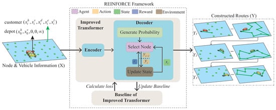
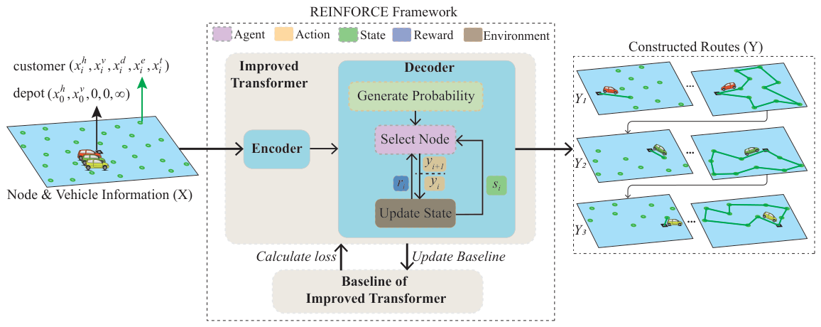
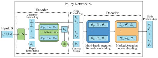
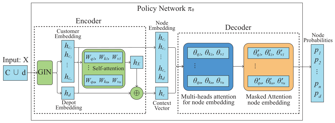
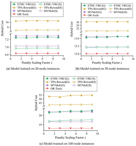
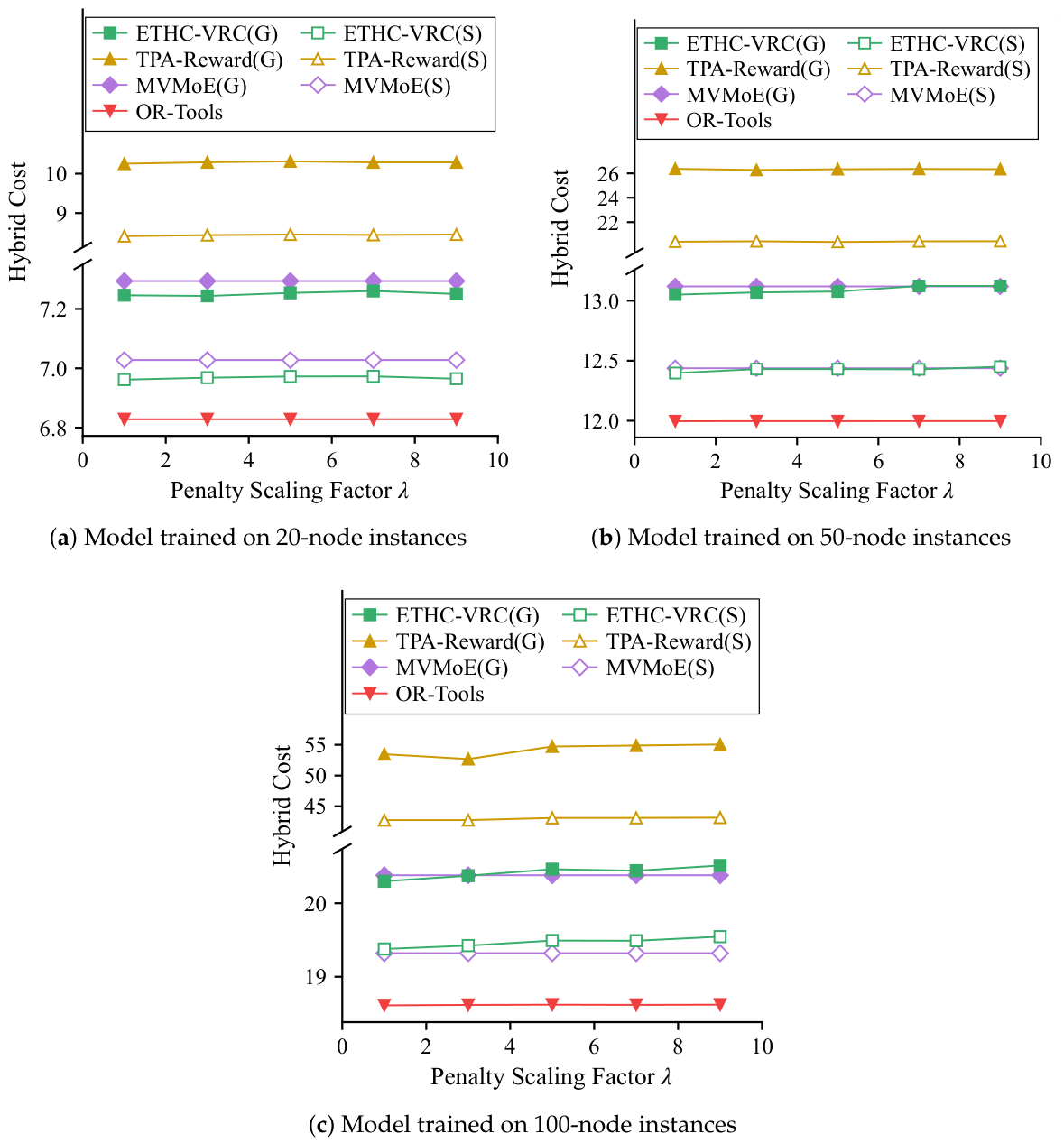
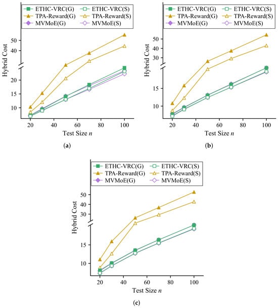
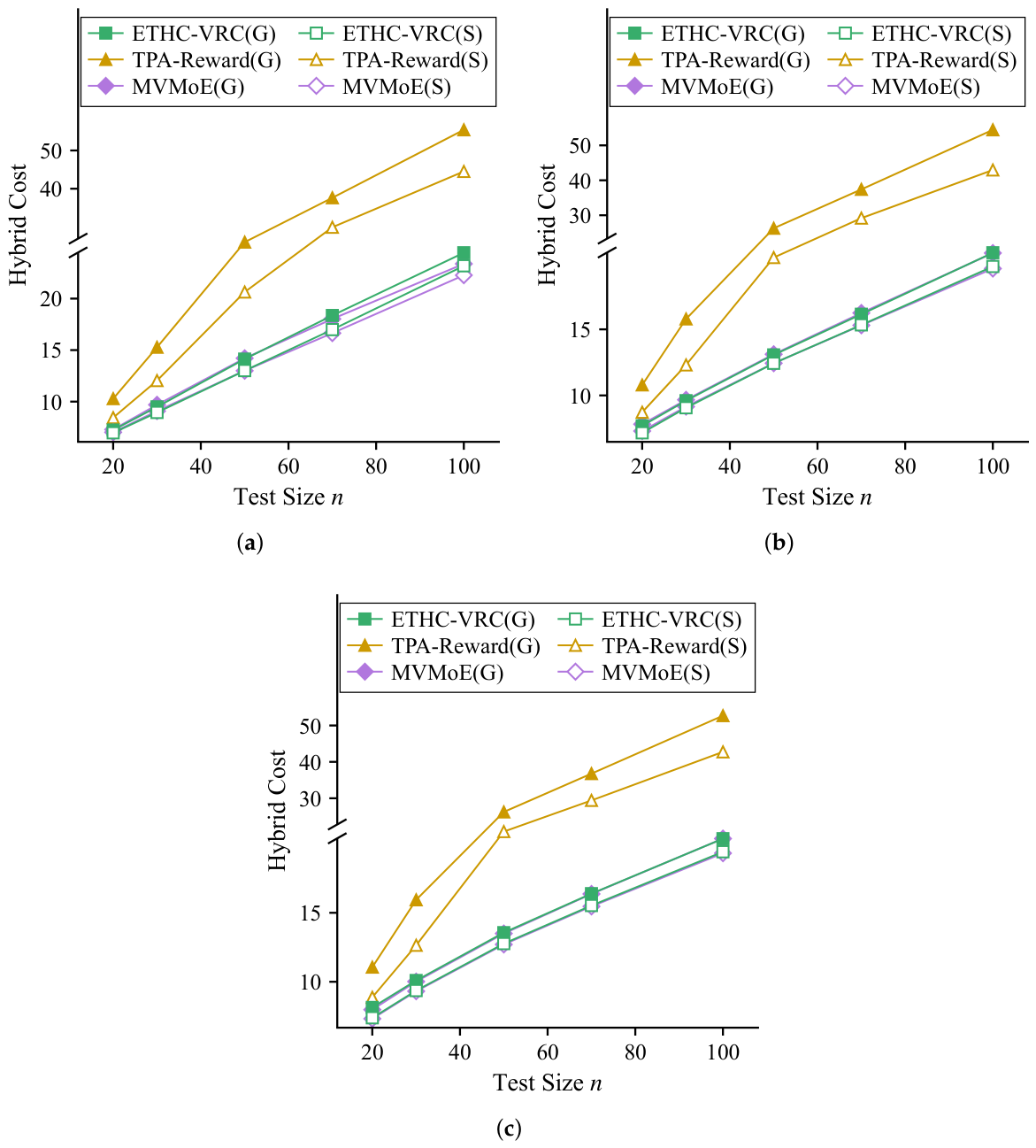
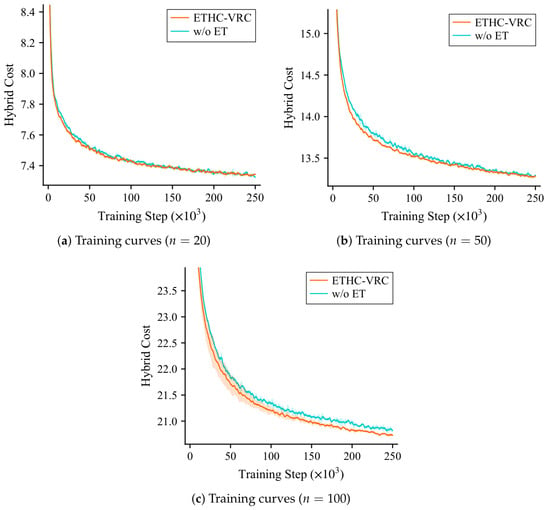
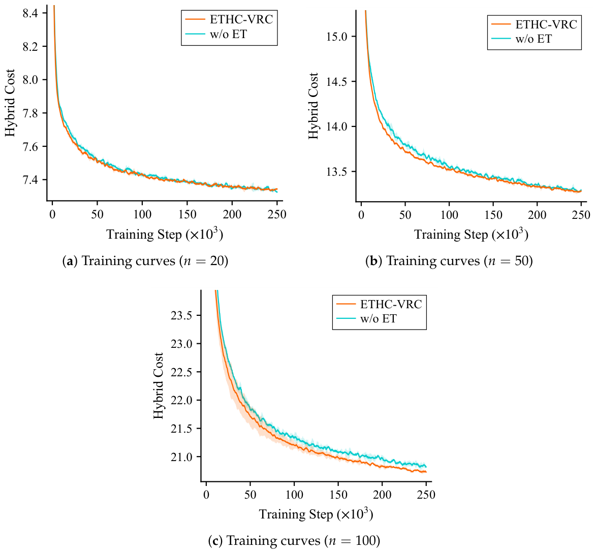
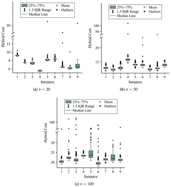
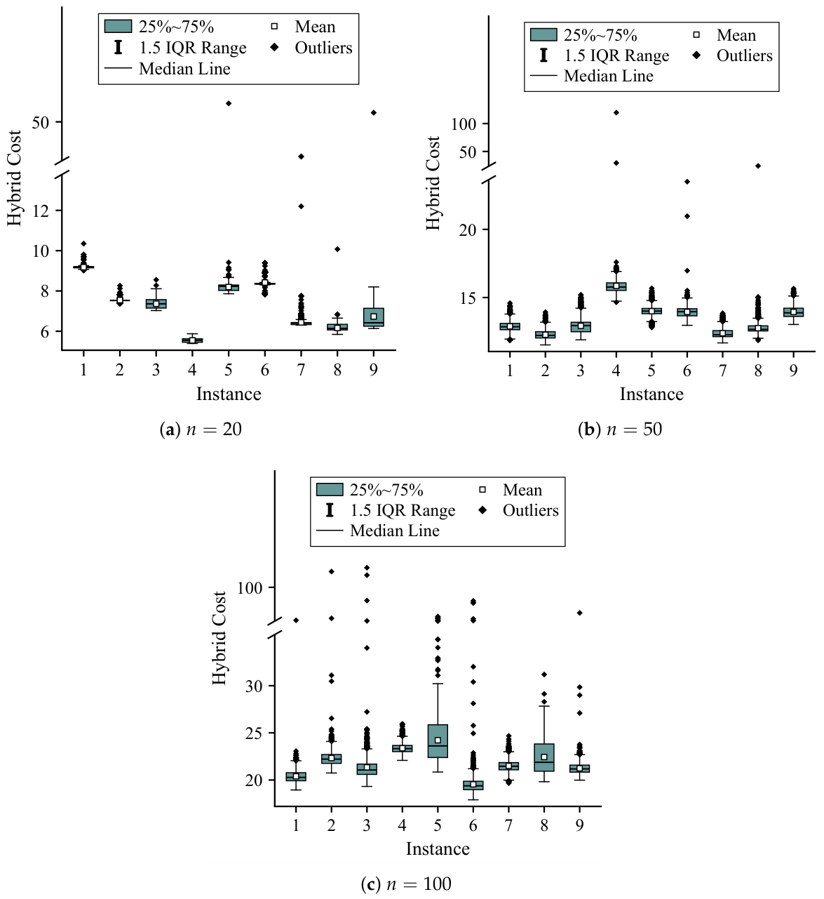

Disclaimer/Publisher’s Note: The statements, opinions and data contained in all publications are solely those of the individual author(s) and contributor(s) and not of MDPI and/or the editor(s). MDPI and/or the editor(s) disclaim responsibility for any injury to people or property resulting from any ideas, methods, instructions or products referred to in the content. |
© 2026 by the authors. Licensee MDPI, Basel, Switzerland. This article is an open access article distributed under the terms and conditions of the Creative Commons Attribution (CC BY) license.