Causal Multivariate Forecasting of Diesel Hydrotreating Variables on a Reproducible Synthetic Benchmark

Abstract

This study evaluates a causal, six-target, 30 min forecasting component for diesel hydrotreating using campaign-separated synthetic data, not a deployed digital twin. An empirical, engineering-constrained simulator generated 30 original campaigns; the recovered code reproduced their datasets byte-for-byte but the simulator did not implement mechanistic balances. The archived AURA-SSM hybrid combines a frozen Ridge anchor, a released measurement observer, multiscale context, bounded corrections, and conditional empirical risk weights; despite its identifier, it has no learned state-space layer. On two previously inspected evaluation domains, frozen NRMSE was 0.16996 and 0.18085, versus ten-degradation means of 0.19170 and 0.20490. These retrospective improvements over leading frozen controls were below the prespecified 3% practical threshold; adaptive Ridge was more accurate on average. Additional matched controls, CRISP/TimeFormer adaptations, and a prespecified 16-campaign synthetic evaluation clarified limitations. On new common/modified simulator structures, AURA-SSM achieved ten-degradation NRMSE of 0.18804/0.20332, outperforming NLinear but not a fixed convex blend; context LightGBM was more accurate with clean measurements. A separately corrected observer passed causal tests and improved prolonged-outage prediction without replacing archived results. Interval undercoverage, lack of mechanistic validation, and absent independent industrial data constrain applicability.

1. Introduction

Digital twins in process engineering integrate computational representations with process data for monitoring, forecasting, optimization, and control [1,2,3,4]. A forecasting algorithm is an enabling component rather than a complete digital twin when bidirectional synchronization with an operating asset has not been demonstrated. This distinction is important for diesel hydrotreating: the present study investigates a multivariate forecasting component, not the deployment or industrial validation of a complete plant twin. Recent industrial forecasting studies have further demonstrated the value of hybrid architectures that combine structured autoregressive representations with deep sequence learning for multivariate process variable prediction [5].

The authors’ earlier related study [5] addressed an industrial fluid catalytic cracking time series using a hybrid autoregressive and deep sequence formulation. That work motivates time-dependent industrial prediction but provides neither the diesel hydrotreating trajectories nor the fitted components evaluated here. The present contribution concerns an empirical hydrotreating simulator, release-time-aware preprocessing, and bounded quality-conditioned allocation of two frozen residual correction directions, supported by dedicated comparator and intervention tests.

Hybrid modeling combines complementary representations to address incomplete mechanistic knowledge and unreliable extrapolation by purely data-driven models [6,7]. Engineering knowledge can enter through constraints, architectural organization, or residual correction rather than only through differential equations [8]. Hydrotreating applications include kinetic–neural integration, multi-output Gaussian process surrogates, dynamic sulfur soft sensors, and virtual sensors for automated control [9,10,11,12]. Related studies address multi-objective product property prediction, sulfur removal optimization, and catalyst grading [13,14,15]. These tasks motivate richer process representations, but soft sensing, catalyst modeling, and optimization are not equivalent to forecasting a future multivariate plant state.

Adaptive and just-in-time soft-sensor studies emphasize operating regime changes, analyzer delays, and limited access to reference measurements [16,17]. Time-series forecasting offers recurrent, convolutional, Transformer, multilayer perceptron, and state-space approaches, without a general guarantee that greater complexity improves a particular process forecast [18]. PatchTST, TimesNet, iTransformer, and S-Mamba illustrate different treatments of temporal context and inter-variable structure [19,20,21,22]. They are relevant to the methodological context; the present comparison uses the specific compact implementations listed in Table 1 rather than claiming to reproduce every architecture reviewed.

Table 1. Forecasting models, representations, and fixed configurations.

Model	Family	Representation	Fixed Configuration
Train Mean	Control	Train target means	6 stored means
Persistence	Control	Last available output	No learned parameters
Ridge	Linear	Full window 24 × 45	α = 100, SVD
Random Forest	Bagging	180 summary features	160 trees; depth 18; leaf ≥ 3
Extra Trees	Randomized bagging	180 summary features	160 trees; unrestricted depth; leaf ≥ 5
LightGBM	Boosting	180 summary features	6 heads; 100 trees/head; 7 leaves; lr 0.05
MLP	Neural	180 summary features	180–96–48–6; lr 0.0012
NLinear	Linear neural	Centered 24 × 45	6486 parameters; lr 0.0005
GRU	Recurrent	Full sequence	Hidden 48; lr 0.002
LSTM	Recurrent	Full sequence	Hidden 48; lr 0.002
TCN	Causal convolutional	Full sequence	48 channels; kernel 3; dilations 1/2/4; lr 0.0005
Transformer	Attention	Full sequence	d = 48; 4 heads; FF = 96; 2 layers; dropout 0.05; lr 0.002
PatchTST-Lite	Patch transformer	6 patches × 4 steps	d = 48; 2 layers; lr 0.002
Compact ANFIS	Neuro-fuzzy	180 → 32 → 8	12 rules; lr 0.0005
GRU-D	Missingness-aware RNN	Values + masks + ages	hidden 48; learned decay; lr 0.0012
TSMixer-Lite	MLP-mixer	24 × 45	2 residual mixer blocks; lr 0.0005
Diagonal SSM	State-space comparator	24 × 45	projection 32; fast/slow diagonal filters; lr 0.0008
Evolving Neuro-Fuzzy Network	Evolving fuzzy	180 → PCA-8	novelty 6; forgetting 0.997; max 24 rules
Diverse Mean Ensemble	Fixed ensemble	Predictions of 4 models	NLinear + GRU + Extra Trees + Compact ANFIS
AURA-SSM	Causal hybrid	Anchor + observer + multiscale context + risk allocation	Ridge anchor α = 10; Ridge observer α = 10; 6 LightGBM × 120 trees; half-life 1; trends 4/12; λr = 0.01; isotropic risk regularization, Equation (19)

Measurement availability is itself informative. Methods for irregular time series distinguish numerical reconstruction from models that explicitly use masks and elapsed times [23]. Similarly, accurate point predictions do not establish reliable uncertainty estimates [24]. Multidimensional and multistep conformal approaches address predictive regions under temporal dependence [25,26], but calibration transfer remains a separate issue when operating regimes or measurement quality change.

The objective is a single-endpoint, six-target causal forecast 30 min ahead under campaign variation, limited sensor availability, and delayed target release. The reported AURA-SSM is a hybrid combination of ordinary regression and fixed causal descriptors, not a mechanistic process model, a new trainable state-space system, or an installed plant twin. The original 19-comparator comparison is retained as retrospective evidence; matched feature/regularization controls, two adapted contemporary forecasting architectures, and subsequently generated synthetic cohorts serve as distinguishable additional evaluations. Accuracy, stress robustness, calibration, statistical evidence, computational requirements, and known counterexamples are interpreted separately.

2. Materials and Methods

2.1. Data and Forecasting Task

The benchmark consists of author-generated, literature-informed synthetic trajectories produced by a reproducible empirical dynamic simulator, not a measured industrial historian or a kinetic first-principles model. Published hydrotreating studies supply process context [11,27,28]; the experimental dibenzothiophene and reaction databases [29,30] were not used as the time-series training data. The developed model consists of 25,200 observations in 14 campaigns, sampled every 5 min and covering eight scheduled operating scenarios. Recovered executable generation definitions reproduce the 30 original Development, Locked, and External campaigns, including all three dataset byte hashes; this establishes provenance and computational replay, not validation of chemical kinetics or conservation laws.

For each input coordinate j, the latent simulated state follows a bounded autoregressive set-point update x_j,t = clip(ϕ_j, ·, x_j,t−1 + (1 − ϕ_j) · s_j,t + ε_j,t L_j U_j). The input persistence coefficients span 0.95–0.985. The nine input bound pairs (L, U), in channel order and their physical units, are: feed flow [55, 155] m³/h; feed temperature [210, 330] °C; feed sulfur [1500, 16,000] mg/kg; hydrogen supply [3500, 19,000] Nm³/h; hydrogen pressure [1.4, 6.0] MPa; reactor temperature [305, 405] °C; reactor pressure [2.2, 7.5] MPa; furnace duty [4, 28] MW; and recycle flow [7000, 39,000] Nm³/h. A further latent constraint enforces hydrogen pressure at least 0.25 MPa below reactor pressure before measurement defects are injected.

The empirical severity is an explicitly defined simulator quantity, not a kinetic rate law. For campaign c and time t, the values are computed as

$${\xi }_t=k_c\hspace{0.17em}{a}_t^{\mathrm{cat}}\exp \left({\displaystyle \frac{{\theta }_t-350}{{\tau }_c}}\right)P_t^{p_c}{H}_t^{h_c}\hspace{0.17em}{\displaystyle \frac{0.82+0.18R_t}{1+0.70f_t}}\hspace{0.17em}{\kappa }_t$$

(1)

Here a_t^cat and f_t are the dimensionless simulated catalyst activity and fouling states, θ_t is the thermal state in °C, and τ_c is the campaign-specific temperature scale. The normalized hydrogen/feed, hydrogen pressure, and recycle factors are H_t, P_t, and R_t; Q_t is the normalized feed flow. Their implemented definitions are

$$H_t=\mathrm{clip}\left({\displaystyle \frac{F_{\mathrm{H}2,t}}{105F_{\mathrm{feed},t}}},0.35,1.8\right), P_t=\mathrm{clip}\left({\displaystyle \frac{P_{\mathrm{H}2,t}}{3.9}},0.45,1.7\right)$$

(2)

$$(R_t=\mathrm{clip}\left({\displaystyle \frac{F_{\mathrm{recycle},t}}{22800}},0.35,1.7\right), Q_t={\displaystyle \frac{F_{\mathrm{feed},t}}{100}}.$$

(3)

Feed flow is expressed in m³/h, hydrogen and recycled gas flows in Nm³/h, and hydrogen pressure in MPa. The thermal state follows Equation (S3), with reactor temperature in °C and furnace duty in MW, and is initialized at the initial reactor temperature. The four campaign coefficients are drawn as

$$k_c^{\left(0\right)}=2.85\exp \left(Z_{k,c}\right), Z_{k,c}\sim \mathcal{N}\left(0,{\left(0.10u_c\right)}^2\right)$$

(4)

$${\tau }_c=37.0\exp \left(Z_{T,c}\right), Z_{T,c}\sim \mathcal{N}\left(0,{\left(0.08u_c\right)}^2\right)$$

(5)

$$h_c=0.42+Z_{h,c}, Z_{h,c}\sim \mathcal{N}\left(0,{\left(0.04u_c\right)}^2\right)$$

(6)

$$p_c=0.53+Z_{p,c}, Z_{p,c}\sim \mathcal{N}\left(0,{\left(0.04u_c\right)}^2\right)$$

(7)

The normal distributions above are parameterized by mean and variance; u_c is the generator’s dimensionless campaign shift level. For the ordinary simulator structure, k_c = k_c⁽⁰⁾ and κ_t = 1. For the modified structure, the additional campaign draw and time-dependent multiplier are

$$k_c=k_c^{\left(0\right)}\exp \left(Z_{s,c}\right), Z_{s,c}\sim \mathcal{N}\left(-0.04,{0.12}^2\right)$$

(8)

κ_t = 1 + 0.10tanh(4(Q_t − 1))

(9)

The sulfur removal fraction is clip(1 − exp(−ξ_t), 0.72, 0.9994), and the sulfur-equilibrium target is max[3, feed sulfur × (1 − removal fraction) + 2.5 + 15f_t]. Hydrogen consumption, pressure loss, product temperature, yield, and density follow their distinct empirical algebraic dependencies and feasibility bounds. Outputs are updated as y[t] = a y[t − 1] + (1 − a)y_eq[t] + correlated-noise[t], where the output inertia coefficient a is clipped to [0.78, 0.94] in the ordinary structure and [0.80, 0.96] after structural perturbation. These executable relations and draws, detailed in Supplementary Section S14 and Table S47, establish computational reproducibility, not identified kinetics, hydraulic laws, or conservation balances.

Scenario trajectories use the smooth transition r = p²(3 − 2p) within eight ordered segments (normal, high feed sulfur, high throughput, hydrogen limitation, reactor temperature drift, recycled gas degradation, catalyst fouling, and combined disturbance). At r = 1, the imposed deviations include, respectively, feed sulfur +3000 mg/kg and hydrogen flow +500 Nm³/h; feed flow +18 m³/h; hydrogen flow −3000 Nm³/h and pressure −0.75 MPa; reactor temperature +18 °C; recycle flow −6200 Nm³/h; an additional fouling forcing term; and combined flow +12 m³/h, sulfur +1800 mg/kg, hydrogen flow −1800 Nm³/h, hydrogen pressure −0.45 MPa, reactor temperature +12 °C, and recycle flow −3200 Nm³/h. Additional correlated forcing and sensor defects are simulated separately. Full input/output bounds, scenario offsets, and deterministic provenance checks are reported in Supplementary Sections S1 and S14.

Latent output coordinates are finally bounded by product sulfur [0, feed sulfur] mg/kg, hydrogen use [0, 0.90, hydrogen supply] Nm³/h, pressure drop [0.01, min (1.2, 0.35, reactor pressure)] MPa, product temperature [180, reactor temperature − 2] °C, yield [80, 100] wt.%, and density [760, 920] kg/m³. Measurement-level spikes, missingness, and stuck-channel defects are introduced after latent generation and can violate the latent pressure ordering. No reactor geometry, residence time law, species-resolved mass balance, enthalpy balance, or independently estimated catalyst kinetics is encoded; consequently, the benchmark is described as empirical and engineering-constrained; its plausibility limits do not establish mechanistic physical validation.

The nine process inputs comprise feed flow, feed temperature, feed sulfur content, hydrogen flow and pressure, reactor temperature and pressure, furnace duty, and recycled gas flow. The six forecast targets are product sulfur, hydrogen consumption, pressure drop, product temperature, diesel yield, and density. Historical target observations can enter the model only after their release. Each example contains 24 causal states; the sole forecast endpoint is six steps later, equivalent to 30 min. The 24 timestamps span 115 min from first to last; the window is conventionally described as a 120 min lookback.

Entire campaigns are assigned to separate functions. Train comprises six campaigns and 10,800 raw rows, producing 10,626 valid windows. Selection uses four other campaigns and 7200 rows, producing 7084 windows. Calibration uses the remaining four campaigns, likewise producing 7084 windows from 7200 rows. Neither overlapping windows nor adjacent rows from a campaign are distributed across these roles. Only the Train function estimates preprocessing parameters.

Locked and External each contain eight campaigns, 17,600 raw rows, and 17,368 forecast origins. Both domains were inspected during earlier development and remain retrospective simulator domain evaluations, not unseen industrial tests; External means a shifted simulation configuration, not a separate refinery. Noise, missingness, stuck values and delayed measurement release alter available histories without changing future scoring targets. A subsequent evaluation, specified before generating the evaluated trajectories, adds two disjoint eight-campaign simulator cohorts (one with the original structural relations and one with modified structure), providing 34,736 further forecast origins. Their new campaign seeds and fixed evaluation policy were not used for model fitting or choice, but their simulator family remains shared with Development. Definitions and original audits remain in Supplementary Sections S1 and S2; additional provenance and cohort details are given in Sections S14–S17.

2.2. Causal Preparation and Information Availability

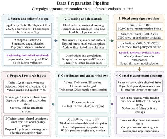
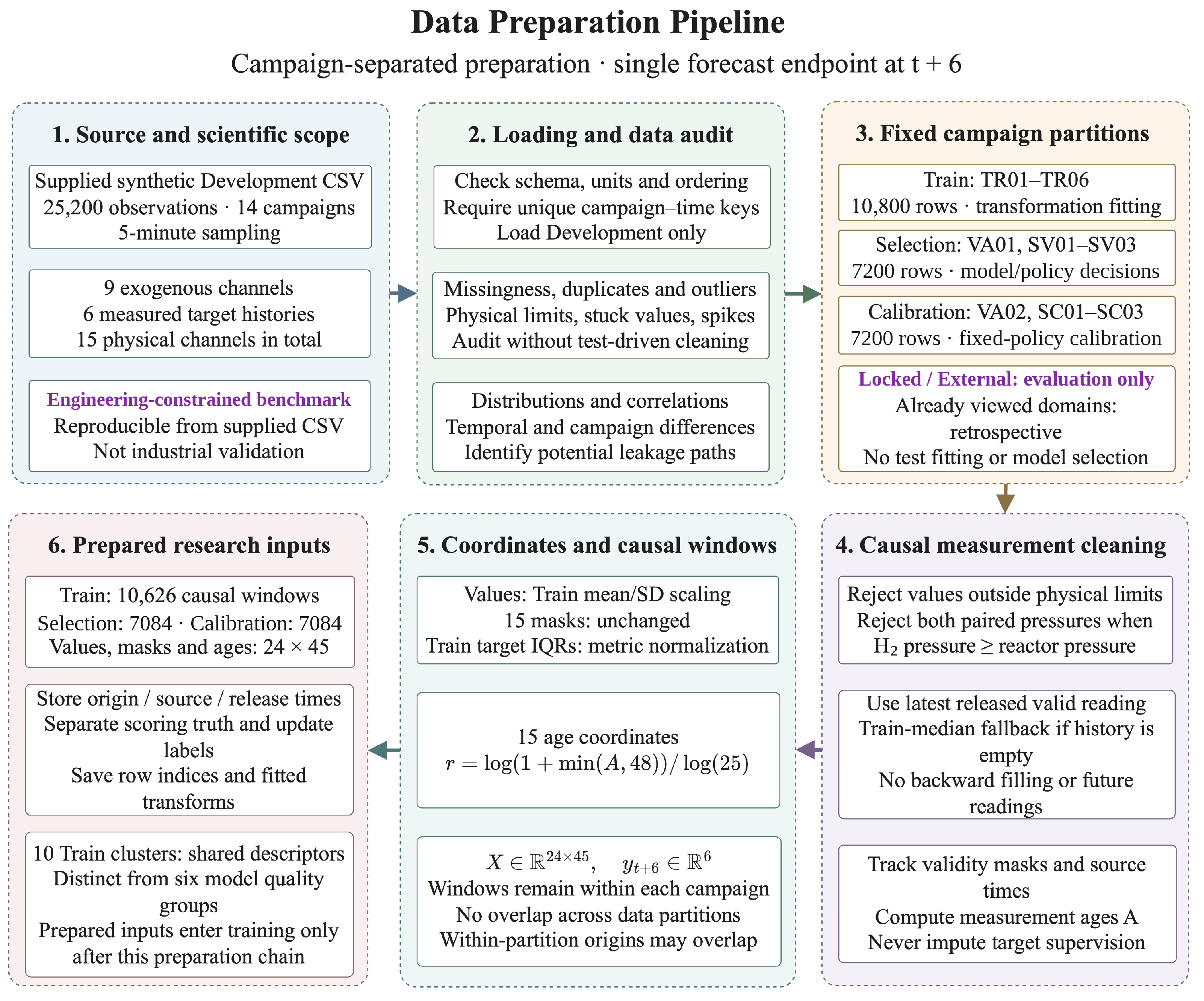
Figure 1 summarizes the campaign-separated preparation chain. Let the original process state at time t be

c_t = [u_t,y_t] ∈ ℝ¹⁵, u_t ∈ ℝ⁹, y_t ∈ ℝ⁶,

(10)

Figure 1. Campaign-separated causal data preparation for multivariate hydrotreater forecasting. Only Train campaigns determine fitted transformations; Selection and calibration have separate roles. The evaluation domains are retrospective, not independent industrial data.

Here, u_t contains the nine process inputs and y_t the six outputs. Schema, units, ordering, unique campaign–time keys, missingness, and physical consistency are audited before modeling. The admissibility indicator for a channel is

$$v_{t,j}=\{\begin{array}{cc}1,& c_{t,j}\in [L_j,U_j]\mathrm{and\; finite},\\ 0,& \mathrm{otherwise},\end{array}$$

(11)

The limits L_j and U_j are predefined. Both paired pressure readings are rejected when the hydrogen pressure is not below the reactor pressure. Process anomaly labels are not used to clean the observations. The latest valid source that has been released by the current time is

s_t,j = max{τ ≤ t − d_j:v_τ,j = 1},

(12)

The delay d_j controls availability, not the scoring target. The latest released valid reading is carried forward; a Train median fallback is used only when no earlier valid reading exists. Neither backward interpolation nor future observations are allowed. The valid arrival mask m_t,j is retained together with measurement age:

For a target channel j, the reference vector 𝓁_t, which is used below in the increment formulation and in the Ridge anchor, is the same actual last-released output, not the last nominal timestamp if its analyzer result is unavailable. The original archived observation feature implementation can instead use an inconsistent fallback when a channel has no released observation within the 24-step window, even if an older valid value exists. This edge case was identified under prolonged outages; the original scoring artifacts are preserved, while a separately evaluated corrected observer uses the carried last-released value for its levels, current reference, and empty history trend fallback. The exact consistency was tested at additional delays of 0, 6, and 12 steps (Supplementary Section S15).

A_t,j = t − s_t,j.

(13)

Values use Train means and standard deviations, while age is capped and transformed logarithmically:

$$z_{t,j}={\displaystyle \frac{{\widehat{c}}_{t,j}-{\mu }_j^{\mathrm{Tr}}}{{\sigma }_j^{\mathrm{Tr}}}},r_{t,j}={\displaystyle \frac{\ln \hspace{0.17em}\left(1+\min (A_{t,j},48)\right)}{\ln \left(25\right)}}.$$

(14)

The standardized values, masks, and age coordinates form the step representation

e_t = [z_t,m_t,r_t] ∈ ℝ⁴⁵.

(15)

and each campaign-contained example is

$$X_t=[e_{t-23},\dots ,e_t]\in {\mathbb{R}}^{24\times 45},y_{t+6}^{*}\in {\mathbb{R}}^6,$$

(16)

Target supervision is never imputed. Target scaling is estimated on Train, and the target-specific interquartile ranges are retained for cross-target error normalization:

$$\mathit{IQ}{R}_k^{\mathrm{Tr}}=Q_{0.75}\left(y_k^{\mathrm{Tr}}\right)-Q_{0.25}\left(y_k^{\mathrm{Tr}}\right)$$

(17)

Origins, measurement source times, and release times are preserved, with scoring truth separated from labels eligible for later updates. Ten clusters obtained from Train-only summary descriptors and an eight-dimensional PCA projection describe proximity to training regimes; they are not physical regime labels and are distinct from the six quality groups used by AURA-SSM. Prefix and future perturbation checks assess causal feature construction. Supplementary Figures S1–S9 document distributions, temporal dependence, campaign shifts, the handling of a missing reading, and past change associations.

2.3. Comparators and Training

Table 1 lists all 20 forecasting solutions. Train mean and persistence are unfitted controls; the remaining comparisons cover regularized regression, tree ensembles, neural architectures, state-space and neuro-fuzzy approaches, and a fixed heterogeneous ensemble. For most fitted methods, the forecast is learned as an increment from the last causally available output vector 𝓁_t ∈ ℝ⁶:

$$\Delta y_t^{*}=y_{t+6}^{*}-{𝓁}_t,{\widehat{y}}_{t+6}={𝓁}_t+f_{\theta }\left(X_t\right).$$

(18)

Ridge uses the vectorized causal window. Tree models and MLP use the 180-dimensional summary of the latest state, mean, standard deviation, and endpoint change:

$${\mathsf{\varphi }}_t=\mathrm{concat}\left({\mathrm{e}}_t,{\overline{\mathrm{e}}}_t,{\mathrm{SD}}_0\left(X_t\right),{\mathrm{e}}_t-{\mathrm{e}}_{t-23}\right)\in {\mathbb{R}}^{180}.$$

(19)

Concatenation is along the feature axis in the stated order. Each of the four blocks has 45 coordinates. For j = 1, …, 45, the temporal mean and population standard deviation are

$${\overline{e}}_{t,j}={\displaystyle \frac{1}{24}}{\displaystyle {\sum }_{k=0}^{23}}{e}_{t-k,j}, {\left[{\mathrm{SD}}_0\left(X_t\right)\right]}_j=\sqrt{{\displaystyle \frac{1}{24}}{\displaystyle {\sum }_{k=0}^{23}}{\left(e_{t-k,j}-{\overline{e}}_{t,j}\right)}^2}$$

(20)

The divisor is 24 (ddof = 0), not 23. Thus, a 24 × 45 causal window maps to exactly 180 summary features. Independent numerical agreement is reported in Supplementary Section S19.3, Table S62.

Regularized multi-output regression is fitted as

$$\widehat{W}=\arg \underset{W}{\min }{\parallel \Delta Y-\mathit{ZW}\parallel }_F^2+\alpha \parallel W{\parallel }_F^2,$$

(21)

The neural models were trained with AdamW, batch size 256, weight decay 2 × 10⁻⁵, gradient-norm clipping at 1, a maximum of 32 epochs, and patience 7. Random Forest and Extra Trees use 160 trees, whereas LightGBM fits six target-specific heads with 100 trees each. NLinear centers physical values on the latest state and retains masks and ages. GRU and LSTM have hidden dimension 48; TCN uses causal dilations 1, 2, and 4. Transformer uses dimension 48, four heads, two encoder blocks, and causal masking. PatchTST-Lite is a six-patch compact adaptation, not a reproduction of the original channel-independent model. Diagonal SSM uses fast and slow stable diagonal filters and is not S4 or Mamba.

Neural fitting uses the common increment loss

$$\mathcal{L}\left(\theta \right)={\displaystyle \frac{1}{6N}}{\displaystyle {\sum }_{i=1}^N}{\displaystyle {\sum }_{j=1}^6}{𝓁}_{\beta }\left({\left[f_{\theta }\left(X_i\right)\right]}_j-{\delta }_{i,j}\right), \beta =0.35.$$

(22)

Here δ_i,j denotes coordinate j of the observed standardized increment Δy_i^* defined in Equation (9); f_θ returns its predicted increment. The scalar SmoothL1 loss is defined as

$${𝓁}_{\beta }\left(e\right)=\{\begin{array}{ll}{e}^2/\left(2\beta \right),& \left|e\right|<\beta ,\\ \left|e\right|-\beta /2,& \left|e\right|\ge \beta .\end{array}$$

(23)

Equation (12) averages over all N × 6 sample–target coordinates. The epoch loss is the sample-weighted mean of minibatch losses. No model was retrained for this mathematical verification (Supplementary Table S62).

AdamW has a batch size of 256, weight decay 2 × 10⁻⁵, gradient-norm clipping at 1, a maximum of 32 epochs, and patience 7. The four predefined initial learning rates are 0.0005, 0.0008, 0.0012, and 0.002 for each architecture. ReduceLROnPlateau can reduce the current rate within a fit; these scheduler updates are not additional search candidates. The selected rates and existing three-initialization fits are documented in Supplementary Table S59. Configurations are fixed before evaluation with seeds 11, 42, and 77; a best seed is not selected. GRU-D includes age-dependent decay, Compact ANFIS uses 12 softly activated rules after an eight-dimensional projection, and the Evolving Neuro-Fuzzy Network uses PCA-8, novelty threshold 6, forgetting factor 0.997, and at most 24 rules.

The fixed Diverse Mean Ensemble averages its four fitted members:

$${\widehat{y}}_{t+6}^{\hspace{0.17em}\mathit{ens}}={\displaystyle \frac{1}{4}}\sum _{m\in \mathcal{M}}{\widehat{y}}_{t+6}^{\left(m\right)},\mathcal{M}=\left\{\mathrm{NLinear},\mathrm{GRU},\mathrm{Extra\; Trees},\mathrm{Compact\; ANFIS}\right\}.$$

(24)

The configurations and representations differ even when they share the same information boundary. Comparisons therefore concern these fitted implementations, not universal rankings of model families. AURA-SSM is a hybrid of linear and tree-based residual components with a constrained combination; the name does not imply an additional deep-neural or selective state-space implementation. Supplementary Tables S13 and S14 provide developmental accuracy and seed repeatability results.

The original fitted controls are not a matched capacity ranking of entire algorithm families. Additional one-factor comparisons independently vary Ridge penalty α ∈ {10,100}, last-state centering, and 15 versus 45 causal features. The nonlinear comparison matches six LightGBM heads, 120 trees per head, a maximum of seven leaves, and a shared training budget, while changing only feature representation or prediction target. In parallel, bounded risk allocation is compared with residual-only correction, fixed convex mixing, and an explicit dynamic heuristic using the same stored correction directions (Supplementary Section S16).

Two additional compact, causal endpoint controls implement the identified operator patterns of CRISP and TimeFormer rather than claiming exhaustive reproduction of their original task settings. Both accept the same 24 × 45 history and predict six outputs at t+6. CRISP preserves multiscale temporal extraction with sparse entmax attention; TimeFormer uses multiscale patch attention and temporal convolutional modulation. Both receive the common AdamW training protocol, four fixed learning rates, up to 32 epochs, batch size 256, and seeds 11, 42, and 77. The TimeFormer source attribution is less conclusive than CRISP, so the comparison is restricted to the checked computational adaptation, not an assertion of official code provenance.

2.4. Hybrid AURA-SSM Forecasting Architecture (Descriptive Model Identifier)

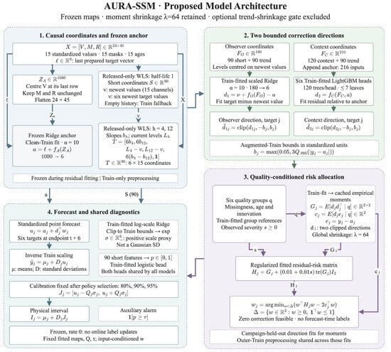
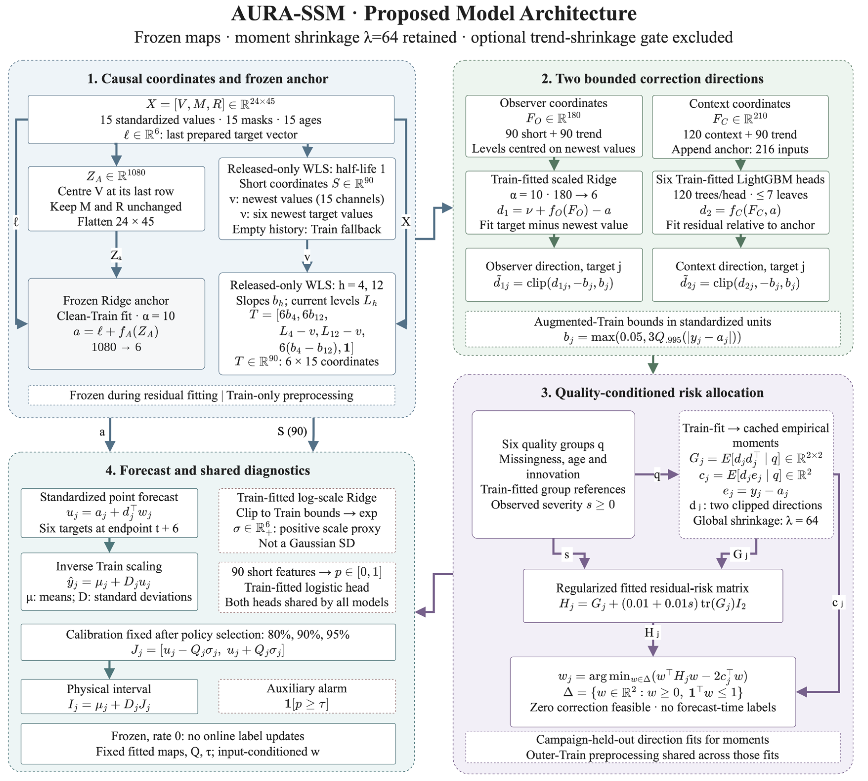
Figure 2 presents the final AURA-SSM architecture as a system for controlled refinement of a stable anchor forecast. An additional nonlinear model does not unconditionally replace the baseline. A fixed linear anchor is first constructed, two bounded correction directions are then formed separately, and their admissible contributions are determined from the estimated residual risk and current observation quality.

Figure 2. AURA-SSM architecture. A frozen Ridge anchor is refined by bounded observer and contextual directions through quality-conditioned empirical risk allocation. Moment shrinkage is retained at λ = 64; the optional trend-shrinkage gate is excluded. Shared interval-scale and anomaly heads do not alter point predictions.

For terminology, AURA denotes availability-aware, uncertainty-regularized residual allocation. The retained identifier “AURA-SSM” is the name under which the original computations and artifacts were registered; its SSM suffix does not describe a separately trained state-space transition or selective SSM layer. The implementation consists of a frozen Ridge anchor, causal observation and multiscale summaries, Ridge/LightGBM correction directions, and an exactly solved two-weight constrained empirical risk problem. A diagonal state-space forecaster remains a distinct comparator in Table 1.

The first block produces the frozen anchor forecast. In X_t, the 15 standardized physical channels are centered on their latest states, while availability masks and measurement ages are left unchanged. The representation is vectorized into Z_A,t ∈ ℝ¹⁰⁸⁰. A Ridge model fitted only to clean Train campaigns predicts the six-dimensional change relative to 𝓁_t:

a_t = 𝓁_t + f_A(Z_A,t), f_A:ℝ¹⁰⁸⁰ → ℝ⁶, α_A = 10.

(25)

The anchor is deliberately kept relatively simple. It provides a stable baseline trajectory that subsequent components may adjust only through bounded corrections.

A causal observer operates in parallel using only released measurements. For each of the 15 channels, it calculates an exponentially weighted level, local slope, dispersion, effective support, age of the newest observation, and innovation between the latest valid readings. The short observer has a half-life of one five-minute step. These descriptors form 90 coordinates. Causal local trends with half-lives of 4 and 12 steps, corresponding to approximately 20 and 60 min, contribute another 90 coordinates. The final configuration retains the multiscale features but excludes the experimental additional cross-scale trend-shrinkage gate.

Causal access and observer computation must be distinguished from the correctness of a particular empty window fallback. In the archived implementation, long target-channel outages revealed disagreement between the carried prediction reference and observer features when the most recent released value lay outside the window. The corrected control is measured separately and does not retrospectively change the original AURA-SSM point forecasts or the fitted parameters reported in the main results.

Two residual correction directions are constructed from these representations. The observation direction uses 180 coordinates and Ridge with α = 10. It first estimates the change in each target relative to its latest causally available measurement and then expresses that estimate as a correction to the anchor:

$${\mathrm{d}}_t^{\left(o\right)}=\mathrm{clip}\left({\mathsf{\nu }}_t+f_O\left({\mathrm{F}}_{O,t}\right)-{\mathrm{a}}_t,\hspace{0.17em}-\mathrm{b},\hspace{0.17em}\mathrm{b}\right).$$

(26)

The vector F_O,t contains 90 short-observer and 90 multiscale coordinates (180 in total). The fitted map f_O includes its Train-fitted feature standardization and Ridge regression with α = 10; its training target is y^* − ν, so ν_t + f_O(F_O,t) is a level forecast and subtraction of a_t produces an anchor-relative correction. The operator clip(z, −b, b) acts coordinate-wise as min[max(z_j, −b_j), b_j]. In the archived observer, ν_t denotes the newest valid in-window target measurement, with the Train-prior fallback when the window contains none. It equals the carried reference 𝓁_t under ordinary supported histories, but can differ after a prolonged outage; the separately corrected observer is not substituted into Equation (15) or the archived scores (Supplementary Section S15, Table S50).

The nonlinear contextual representation F_C,t has 210 coordinates: 120 base-context coordinates and 90 multiscale coordinates. The base context consists of the 90 short-observer coordinates, 15 newest values, and 15 newest-minus-level differences. Appending the six-dimensional anchor produces a 216-coordinate regressor input. The six LightGBM heads are fitted to y^* − a, the residual relative to the anchor, and return the bounded correction

$${\mathrm{d}}_t^{\left(c\right)}=\mathrm{clip}\left(f_C\left(\mathrm{concat}\left({\mathrm{F}}_{C,t},{\mathrm{a}}_t\right)\right),\hspace{0.17em}-\mathrm{b},\hspace{0.17em}\mathrm{b}\right).$$

(27)

Each LightGBM head contains 120 trees, at most seven leaves per tree, and a learning rate of 0.04.

Consequently, f_C is a residual map from 216 coordinates to six anchor-relative outputs. The independent feature and direct-booster comparisons reproduce this mapping exactly on the tested Selection histories (Supplementary Table S62).

Both correction directions are bounded by the same Train-derived limit:

b_j = max[0.05,3 Q_0.995(∣y_j − a_j∣)].

(28)

Neither residual component can therefore move the prediction arbitrarily far from the stable anchor.

The next block allocates residual risk conditionally using six fixed quality groups. Let m_t be the unavailable measurement fraction over the 24 × 15 arrival mask coordinates; A_t^max the largest newest-observation age among the six target channels, measured in five-minute steps; and I_t,j the innovation between the newest and preceding valid released readings of channel j. The Train-only innovation scale and the cross-channel innovation ratio are

$$v_j=\max \left\{Q_{0.95}^{\mathrm{Train}}\left(\left|I_j\right|\right),0.01\right\}, r_t={\mathrm{median}}_{j=1,\dots ,15}{\displaystyle \frac{\left|I_{t,j}\right|}{v_j}}$$

(29)

The quality category c_t is 2 if m_t ≥ 0.075 or A_t^max ≥ 3; otherwise, it is 1 if m_t ≥ 0.01 or A_t^max > 0; otherwise, it is 0. Category 2 therefore takes precedence. Crossing these categories with the strictly defined innovation indicator gives

q_t = 2c_t + 1{r_t > 1} ∈ {0,1,2,3,4,5}.

(30)

The six explicit definitions, including the strict r_t > 1 boundary, are tabulated in Supplementary Table S60; eleven equality and just-below/above boundary cases are reported in Table S61. These criteria are frozen and are not estimated from Selection or evaluation outcomes. For each target j, d_t,j = [d_t,j^(o), d_t,j^(c)]^T contains the two correction directions. Campaign-held-out training predictions determine their second moments and association with the anchor residual:

$$G_{q,j}=\mathbb{E}\left[d_j{d}_j^{\top }\mid q\right],c_{q,j}=\mathbb{E}\left[d_j{e}_j\mid q\right],e_j=y_j-a_j.$$

(31)

To stabilize small groups, conditional moments are shrunk toward global estimates with a fixed equivalent observation count λ_m = 64. This is not an additional online fit; the estimates remain fixed after training.

The nonnegative prediction-time degradation coordinate is defined entirely from the same observation summaries:

$$s_t=\mathrm{clip}\left(m_t/0.1,0,2\right)+\mathrm{clip}\left(A_t^{\max }/3,0,2\right)+\mathrm{clip}\left(r_t-1,0,2\right))$$

(32)

Each term is clipped to [0, 2], so 0 ≤ s_t ≤ 6. Target ages are in sampling steps, not minutes, and neither current scoring truth nor future labels enter s_t. With q_t being the current quality group and G_q,j being the stored second moment matrix after the shrinkage described above, the regularized risk matrix is

$$H_{t,j}=G_{q_t,j}+\left({\lambda }_r+\gamma s_t\right)\mathrm{tr}\left(G_{q_t,j}\right)I_2, {\lambda }_r=\gamma =0.01.$$

(33)

Here, λ_r = 0.01 is the fixed isotropic Ridge multiplier of tr(G_q,j); γ = 0.01 multiplies the additional degradation-dependent penalty γ s_t tr(G_q,j). Both are dimensionless and remain fixed after training. They are distinct from λ_m = 64, which is the equivalent observation count used to shrink conditional moments. Numerical checks of the objective, feasible weights and six independently optimized target-specific cases are reported in Supplementary Table S62.

The weights are obtained by solving a two-dimensional convex problem exactly, rather than through a neural gate:

$$w_{t,j}=\arg \underset{w}{\min }\left(w^{\top }{H}_{t,j}w-2c_{q,j}^{\top }w\right),w\ge 0,1^{\top }w\le 1.$$

(34)

The final constraint has a direct interpretation: the correction weights cannot sum to more than one, and the zero vector is always feasible. When the empirical risk structure does not support either additional direction, AURA-SSM can retain the original Ridge anchor without correction.

The convex weights minimize an estimated penalized squared-loss surrogate using group-conditional empirical second moments. Nonnegativity and a sum not exceeding one guarantee an admissible zero-correction option; they do not guarantee a lower realized error at every forecast origin. The same two previously fitted directions allow a controlled comparison with a constant convex mixture. Under the common new-cohort stress protocol, the constant mixture is slightly better in mean NRMSE, limiting claims that conditional risk allocation is indispensable (Supplementary Section S17, Tables S55 and S56).

The final standardized forecast is formed as

$$u_{t,j}=a_{t,j}+d_{t,j}^{\top }{w}_{t,j},{\widehat{y}}_{t+6,j}={\mu }_j^{\mathit{Tr}}+{\sigma }_j^{\mathit{Tr}}{u}_{t,j}.$$

(35)

A separate diagnostic branch does not participate in calculating ${\widehat{y}}_{t+6}$. From the 90 short causal features, Ridge estimates a positive error-scale proxy and a logistic head estimates the probability of a simulated anomalous state. Once the forecasting policy is fixed, calibration campaigns determine multipliers for nominal levels of 80, 90, and 95%. These procedures affect intervals and diagnostic signals, not the point forecast.

The final frozen configuration of AURA-SSM performs no online parameter updates. The true future state is used neither to issue the current forecast nor to calculate its correction weights. Adaptation using matured delayed labels is evaluated separately as an operating mode and is not a hidden part of the frozen result. AURA-SSM is therefore neither a conventional ensemble nor a neural network with dynamic attention. It is a causally constrained hybrid architecture that refines a stable baseline according to Train-derived evidence about admissible residual risk reduction.

2.5. Evaluation Protocol and Uncertainty Assessment

Model fitting and preprocessing used Train only. Selection determined model configurations and delayed-feedback policies; calibration was accessed only after the point forecast policy was fixed. The main reported run uses seed 42, with seeds 11 and 77 providing additional algorithmic repeatability checks. Locked and External were inspected previously and are therefore retrospective synthetic evaluation domains. Their separation from the current fitting and Selection stages does not make them newly blinded industrial tests.

The previously inspected Locked and External domains are reported only as retrospective descriptive evidence. The later 16-campaign experiment was Locked before fresh generation by recording new campaign seeds, frozen model-state identities, the two simulator structure conditions, ten noise/missing/stuck/delay perturbations, three additional 40-step target outages, and 62 planned paired contrasts. No new-cohort labels were used to train, select, or recalibrate the models. The statistical unit is a generated campaign, with temporally overlapping forecast origins nested within each campaign; all new-domain inferences are conditional on the shared simulator.

Frozen operation retains fitted point model parameters. The adaptive track evaluates each model with its Selection-fixed policy: frozen, global recursive least squares, or gated local memory. A policy may remain frozen, as it did for AURA-SSM. Feedback is used only after the target observation has been released; scoring truth is stored separately from update labels. The same availability rule applies to historical target channels and to permitted delayed updates.

The primary error is the unweighted mean of six target-specific RMSE values divided by their fixed Train interquartile ranges. NMAE and mean target-specific R² are reported separately. Secondary criteria are stabilized MAPE, sMAPE, absolute normalized bias, and violations of predefined channel bounds. Interval evaluation reports marginal coverage, the mean absolute target-wise coverage gap, normalized width, and interval score; near-nominal pooled coverage can conceal undercoverage of individual targets.

A common Train-fitted scale head and anomaly head are shared across forecasters. Calibration determines target-specific interval multipliers at nominal 80%, 90%, and 95% levels after the forecasting policy has been selected. The multiplier calculation uses 240 thinned calibration origins. The scale output is a positive error-scale proxy, not a Gaussian standard deviation. These marginal empirical intervals are not accompanied by a coverage guarantee under temporal dependence or distribution shift.

The calibration quantiles are finite-sample order statistics of target-wise normalized absolute residuals, which is a split-conformal-style score construction on the calibration partition. References [25,26] provide methodological context; their multivariate region constructions are not the interval algorithms implemented here. It is not an exact finite-sample coverage guarantee for dependent, simulator-shifted, or measurement-degraded trajectories. In particular, the separately corrected observer did not eliminate marked undercoverage during severe target outages; no post hoc adjustment using evaluation labels was applied.

The four-condition component comparison averages clean, noise 5%, missing 5%, and an additional six-step target measurement delay. It must not be confused with the final ten-stress mean, which excludes clean. The latter averages three noise levels, three missingness levels, two stuck-channel conditions, and additional target measurement delays of six and twelve steps. The future scoring targets are unchanged. Equal condition weights are descriptive; real operating frequencies of these disturbances were not estimated.

Paired inference distinguishes mean normalized squared-loss differences from differences in macro NRMSE. Campaign-aware, heteroskedasticity- and autocorrelation-consistent inference is combined with Holm adjustment across 152 contrasts. Hierarchical resampling of campaigns and temporal blocks provides pointwise 95% intervals for the NRMSE difference at block lengths of 30, 60, and 120 forecast origins. Joint support requires a favorable adjusted test and positive intervals at all three block lengths; a point estimate of at least 3% additionally defines practical support. These intervals are not simultaneous confidence regions for the entire comparison family.

Computational measurements distinguish a prepared-input point forecast from the complete single-origin online pipeline. Timing uses 200 warmed-up inputs with a batch size of one. Recorded fitting time, serialized point and pipeline states, model structure, and sampled process resident memory describe different resource quantities. Shared-process resident memory is not an isolated peak-memory benchmark for an individual model.

For comparability, new-cohort clean errors summarize the three predefined initializations, whereas the ten-stress and outage protocols use the preselected primary initialization. Frozen forecasts are separated from a common intercept-only recursive least-squares control with gain 0.001; the latter is a matched operational diagnostic and does not redefine AURA-SSM’s original frozen policy. The 3% practical difference criterion is a descriptive threshold distinct from Holm-adjusted significance and campaign/block confidence intervals; the previously inspected domain rankings are not reinterpreted as prospective confirmation.

3. Results

3.1. Data Diagnostics and Developmental Evidence

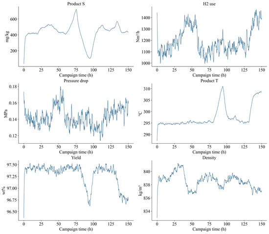
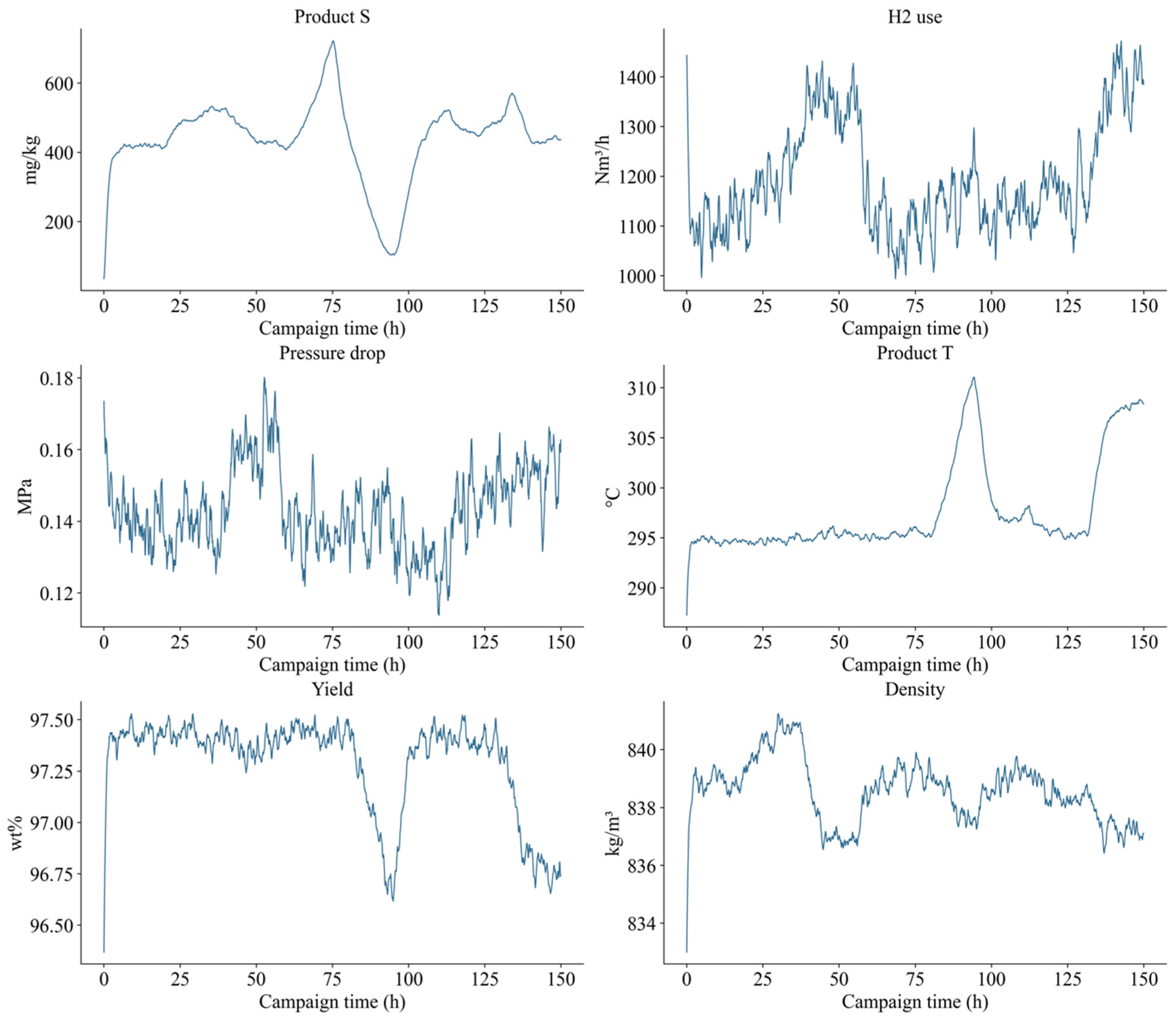
The training audit found 144 missing input measurements and four additional finite readings rejected through the paired pressure constraint. All 148 channel observations were represented by previously released valid values; no Train median fallback was required. Statistical outlier and spike flags were treated as diagnostics rather than automatic deletion criteria. Strong target persistence coexists with campaign shifts: first-lag autocorrelations are approximately 0.99–1.00, yet Selection and calibration contain 28.68% and 20.19% of windows outside the Train-derived support boundary. These descriptors are not out-of-distribution probabilities (Supplementary Tables S1–S12 and Figures S1–S9). Figure 3 shows the time evolution of the six simulated output variables for one representative training campaign.

Figure 3. One simulated training campaign: time evolution of product sulfur, hydrogen use, pressure drop, product temperature, diesel yield, and density. Original simulated trajectory; not an industrial plant record.

The campaign exhibits sustained levels, smooth transitions, and comparatively rapid fluctuations across different output channels. These time scales explain why a last-value baseline can remain competitive over 30 min. The displayed response is generated by a bounded empirical dynamical system and cannot independently establish catalyst kinetics or process plant fidelity.

On the 7084 clean Selection windows, AURA-SSM achieves NRMSE 0.16705, NMAE 0.13264, and mean R² 0.93152. NLinear is the nearest NRMSE comparator at 0.16898, so the relative difference is about 1.14%, which is not a large separation. Across the three specified initializations, AURA-SSM retains the lowest observed error in every run, but NLinear has lower between-seed variability. Selection results characterize model development, not independent testing (Supplementary Tables S13 and S14).

The additional controls reveal a relevant developmental counterexample: a six-head context-matched LightGBM trained on Train and evaluated on the same Selection histories attains NRMSE 0.16494, which is below the archived AURA-SSM value of 0.16705. These additional comparator configurations were not part of the original 19-comparator ranking and thus do not invalidate the earlier table values; they limit the general claim that the hybrid is optimal among all viable fitted alternatives.

3.2. Retrospective Point Forecast Accuracy

Table 2 and Table 3 report the main accuracy measures for all models. F/A denotes frozen operation followed by the selected delayed-feedback policy; a single value denotes identical results. AURA-SSM remains frozen in both tracks. Bold values mark observed within-track optima, not statistical significance. Its frozen NRMSE values are 0.16996 on Locked and 0.18085 on External. The nearest competitor is LightGBM on Locked and NLinear on External; the corresponding relative gains are about 1.57% and 0.69%.

Table 2. Locked prediction accuracy: frozen and selected adaptive policies.

Model	NRMSE, F/A ↓	NMAE, F/A ↓	R2, F/A ↑
AURA-SSM	0.16996/0.16996	0.13527/0.13527	0.92391/0.92391
Train Mean	0.91591/0.44498	0.74624/0.31436	−0.06105/0.72884
Persistence	0.19422	0.15239	0.90860
Ridge	0.18908/0.16756	0.15142/0.13332	0.92111/0.92734
Random Forest	0.18235	0.14403	0.91756
Extra Trees	0.18036	0.14263	0.91941
LightGBM	0.17267/0.17395	0.13742/0.13841	0.92173/0.92065
MLP	0.18781/0.18697	0.14882/0.14781	0.91493/0.91454
NLinear	0.17357	0.13814	0.92054
GRU	0.18778/0.18507	0.14871/0.14598	0.91906/0.92034
LSTM	0.19541/0.18951	0.15513/0.14960	0.91490/0.91601
TCN	0.19368/0.19412	0.15250/0.15245	0.91025/0.90879
Transformer	0.19319/0.19311	0.15214/0.15157	0.91127/0.90998
PatchTST-Lite	0.19533/0.19137	0.15470/0.15105	0.90969/0.91086
Compact ANFIS	0.18457/0.18517	0.14642/0.14661	0.91611/0.91547
GRU-D	0.19664/0.18465	0.15606/0.14564	0.91411/0.91989
TSMixer-Lite	0.17558	0.13954	0.92006
Diagonal SSM	0.19269/0.19278	0.15180/0.15125	0.91166/0.91082
Evolving Neuro-Fuzzy Network	0.25842/0.19974	0.20722/0.15775	0.84036/0.90369
Diverse Mean Ensemble	0.17568	0.13936	0.92278

↓ indicates that lower values are better; ↑ indicates that higher values are better. Bold values indicate the best observed result within the corresponding frozen or adaptive track and do not indicate statistical significance.

Table 3. External prediction accuracy: frozen and selected adaptive policies.

Model	NRMSE, F/A ↓	NMAE, F/A ↓	R2, F/A ↑
AURA-SSM	0.18085/0.18085	0.14348/0.14348	0.94102/0.94102
Train Mean	1.23350/0.66301	0.96558/0.44738	−0.09524/0.67629
Persistence	0.20188	0.15826	0.93174
Ridge	0.28817/0.17874	0.23051/0.14185	0.88314/0.94352
Random Forest	0.19291	0.15171	0.93648
Extra Trees	0.19119	0.15057	0.93782
LightGBM	0.18475/0.18324	0.14653/0.14529	0.93898/0.93955
MLP	0.20262/0.19528	0.16077/0.15423	0.93473/0.93626
NLinear	0.18211	0.14467	0.93929
GRU	0.20840/0.19543	0.16547/0.15420	0.93453/0.93957
LSTM	0.21243/0.20073	0.16852/0.15817	0.93382/0.93638
TCN	0.20551/0.20201	0.16284/0.15894	0.93235/0.93217
Transformer	0.20565/0.20107	0.16248/0.15789	0.93200/0.93290
PatchTST-Lite	0.20786/0.19889	0.16571/0.15706	0.93277/0.93407
Compact ANFIS	0.19654/0.19287	0.15590/0.15234	0.93599/0.93718
GRU-D	0.21222/0.19473	0.17000/0.15361	0.93402/0.93937
TSMixer-Lite	0.18439	0.14638	0.93913
Diagonal SSM	0.20270/0.20038	0.16034/0.15724	0.93314/0.93363
Evolving Neuro-Fuzzy Network	0.31805/0.20736	0.26207/0.16327	0.82633/0.92961
Diverse Mean Ensemble	0.18644	0.14790	0.94066

↓ indicates that lower values are better; ↑ indicates that higher values are better. Bold values indicate the best observed result within the corresponding frozen or adaptive track and do not indicate statistical significance.

Adaptive Ridge is more accurate on both domains, with NRMSE 0.16756 and 0.17874. Adaptation is not uniformly beneficial: some model–domain combinations worsen despite receiving only causally permitted feedback. Target-specific physical errors also differ markedly. Product sulfur RMSE is 4.4195 and 4.8275 mg/kg, whereas pressure drop RMSE is 0.0063519 and 0.0067083 MPa. Pressure drop retains the lowest target-specific R², 0.72505 and 0.75129. All six absolute errors increase on External even though R² increases, because the latter depends on domain-specific target variance (Supplementary Tables S15–S19).

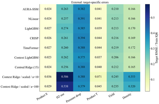
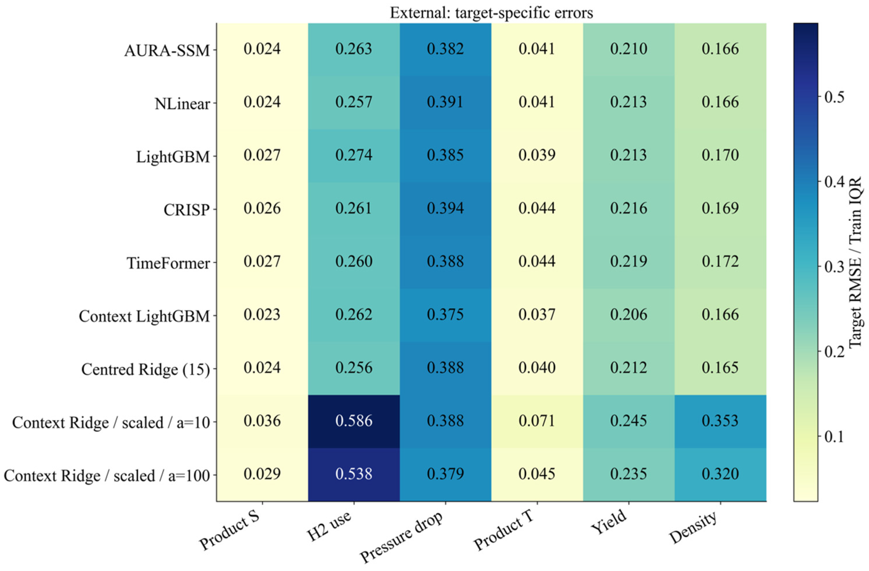
Secondary criteria do not identify the same winner in every case. Frozen AURA-SSM has the lowest percentage errors in both domains, but persistence has smaller absolute bias on External. Adaptive LightGBM attains the smallest External percentage errors, while adaptive Ridge leads in NRMSE. Adaptive GRU produces a 0.010556% rate of out-of-bound target coordinates on External; the other reported combinations have zero violations. Channel-bound compliance is not a process-safety guarantee. Figure 4 compares target-specific normalized errors across AURA-SSM and the additional matched and contemporary forecasting controls on the External evaluation domain.

Figure 4. Target-specific NRMSE relative to Train IQR for the retrospectively evaluated External simulator domain under frozen forecasting. Additional matched and contemporary controls are compared using identical forecast horizons.

White font is used only to improve readability in darker heatmap cells and does not indicate statistical significance or a separate data category.

Target-wise errors expose a different ordering from the six-target macro average. Strong persistence dominates the sulfur and product temperature outputs, while pressure drop and hydrogen consumption errors are much larger after normalization. The results must be read by target and model configuration; small overall advantages do not imply a uniform gain for all six outputs.

3.3. Predictive Uncertainty

Supplementary Tables S20–S23 retain every model and all three nominal interval levels. On clean Locked data, AURA-SSM has the lowest interval score among frozen solutions at 80%, 90%, and 95%, but not the smallest target-wise coverage gap. Its nominal 90% coverage is 90.577%. On External this falls to 87.596%; the 95% interval covers 93.155%. AURA-SSM leads in frozen interval score at 80% and 90%, whereas NLinear is better at 95%. Adaptive Ridge has lower interval scores than AURA-SSM at all three levels on both domains.

Coverage and informativeness must be interpreted jointly. Wide intervals can achieve high coverage while having poor interval scores, and averaging coverage over targets can conceal opposing calibration errors. The scale head is shared across point forecasters, but the calibrated multipliers are policy-specific. None of these finite-sample results establishes exchangeability or guaranteed coverage under shift. Degradation-dependent interval results are retained in Supplementary Tables S24 and S25.

3.4. Measurement Degradation

Table 4 and Table 5 summarize the ten perturbed conditions, excluding clean. AURA-SSM has the lowest frozen mean NRMSE: 0.19170 on Locked and 0.20490 on External. Its gains over the nearest frozen competitor are about 1.56% and 2.18%, which is below the 3% practical threshold. Adaptive Ridge lowers the mean NRMSE further to 0.18833 and 0.20128. In contrast, AURA-SSM retains the smallest worst-condition NRMSE across both tracks: 0.25772 and 0.28550. The preferred method consequently depends on whether the criterion is the average or the most adverse of the tested conditions.

Table 4. Mean and worst errors across ten measurement degradations on Locked.

Model	Mean NRMSE, F/A ↓	Worst NRMSE, F/A ↓	Mean NMAE, F/A ↓
AURA-SSM	0.19170/0.19170	0.25772	0.15208/0.15208
Train Mean	0.91591/0.45411	0.91591/0.49772	0.74624/0.32228
Persistence	0.21888	0.32357	0.17100
Ridge	0.20654/0.18833	0.27151/0.26645	0.16455/0.14886
Random Forest	0.20494	0.29735	0.16098
Extra Trees	0.20342	0.29531	0.15996
LightGBM	0.19473/0.19692	0.27988/0.28853	0.15394/0.15546
MLP	0.21100/0.21159	0.30755/0.31522	0.16626
NLinear	0.21103	0.30951	0.16868
GRU	0.21026/0.20866	0.30379/0.30858	0.16566/0.16363
LSTM	0.21736/0.21357	0.31087/0.31620	0.17160/0.16762
TCN	0.21800/0.21937	0.32125/0.32779	0.17087/0.17137
Transformer	0.21739/0.21824	0.31944/0.32557	0.17039/0.17046
PatchTST-Lite	0.21890/0.21605	0.31738/0.32020	0.17253/0.16961
Compact ANFIS	0.20719/0.20903	0.29967/0.30829	0.16342/0.16450
GRU-D	0.21798/0.20806	0.30782/0.30681	0.17224/0.16325
TSMixer-Lite	0.20284	0.28783	0.16047
Diagonal SSM	0.21665/0.21792	0.31815/0.32592	0.16982/0.17010
Evolving Neuro-Fuzzy Network	0.27710/0.22455	0.35850/0.33172	0.22100/0.17627
Diverse Mean Ensemble	0.20047	0.29432	0.15824

↓ indicates that lower values are better; ↑ indicates that higher values are better. Bold values indicate the best observed result within the corresponding frozen or adaptive track and do not indicate statistical significance.

Table 5. Mean and worst errors across ten measurement degradations on External.

Model	Mean NRMSE, F/A ↓	Worst NRMSE, F/A ↓	Mean NMAE, F/A ↓
AURA-SSM	0.20490/0.20490	0.28550	0.16188/0.16188
Train Mean	1.23350/0.67014	1.23350/0.70478	0.96558/0.45467
Persistence	0.22939	0.35068	0.17897
Ridge	0.30400/0.20128	0.37006/0.29131	0.24213/0.15871
Random Forest	0.21827	0.32652	0.17069
Extra Trees	0.21715	0.32558	0.16999
LightGBM	0.20948/0.20930	0.31086/0.31877	0.16495/0.16458
MLP	0.22772/0.22283	0.33802/0.34410	0.17943/0.17475
NLinear	0.22171	0.33418	0.17661
GRU	0.23307/0.22177	0.34023/0.33824	0.18412/0.17382
LSTM	0.23756/0.22789	0.34847/0.34894	0.18739/0.17850
TCN	0.23215/0.23020	0.35104/0.35607	0.18290/0.18002
Transformer	0.23247/0.22912	0.35040/0.35397	0.18254/0.17892
PatchTST-Lite	0.23370/0.22634	0.34690/0.34715	0.18516/0.17770
Compact ANFIS	0.22109/0.21962	0.32837/0.33586	0.17431/0.17243
GRU-D	0.23620/0.22094	0.34149/0.33670	0.18786/0.17324
TSMixer-Lite	0.21390	0.31420	0.16886
Diagonal SSM	0.22916/0.22844	0.34592/0.35373	0.18010/0.17828
Evolving Neuro-Fuzzy Network	0.33641/0.23489	0.42102/0.35851	0.27536/0.18383
Diverse Mean Ensemble	0.21375	0.32327	0.16849

↓ indicates that lower values are better; ↑ indicates that higher values are better. Bold values indicate the best observed result within the corresponding frozen or adaptive track and do not indicate statistical significance.

This point forecast advantage does not establish interval reliability. Under the most adverse tested degradation, AURA-SSM coverage for nominal 90% intervals falls to 0.73302 on Locked and 0.69195 on External. NLinear undercovers still more severely, but a better relative ranking does not remove the absolute calibration failure. Equal weighting of simulated disturbances is a descriptive stress benchmark, not an estimate of real industrial risk (Supplementary Tables S24 and S25).

3.5. Component Effects and Statistical Support

The transferred component interventions distinguish nominal fit from robustness (Supplementary Tables S26 and S27). Removing augmentation slightly improves clean error but worsens the four-condition mean by 6.72730% on Locked and 5.38780% on External, with worsening in all three runs. Removing the contextual or observation direction also worsens that mean. Multiscale trends have a smaller robustness benefit but are not uniformly better on clean data. The reliability penalty is practically neutral and its removal slightly improves the four-condition score. These findings support the main correction scheme without establishing that every auxiliary mechanism is necessary.

Table 6 classifies the paired evidence; Supplementary Tables S28–S31 retain the adjusted tests and all three block-length intervals. Adaptive Ridge has supported advantages on both domains. Several close contrasts remain unresolved under the joint rule. On External, the clean NLinear NRMSE intervals include zero despite a significant squared-loss test. The clean adaptive LightGBM contrast depends on block length. For frozen LightGBM on Locked, the ten-stress squared-loss contrast is not significant after correction, although the NRMSE intervals are positive. The two statistical functionals must therefore not be treated as interchangeable.

Table 6. Joint statistical and practical evidence classification for AURA-SSM comparisons.

Domain	Mode	Conditions	Comparator Advantage	Supported Gain ≥ 3%	Small Supported Gain	Unresolved
External	Adaptive	Clean	1	15	1	2
External	Adaptive	Ten stresses	1	17	1	0
External	Frozen	Clean	0	16	2	1
External	Frozen	Ten stresses	0	18	1	0
Locked	Adaptive	Clean	1	16	2	0
Locked	Adaptive	Ten stresses	1	17	1	0
Locked	Frozen	Clean	0	17	2	0
Locked	Frozen	Ten stresses	0	18	0	1

3.6. Diagnostics, Heterogeneity, and Computational Cost

The common anomaly head is not an AURA-SSM-specific advantage. AUROC decreases from 0.74810 on Locked to 0.65942 on External, while false alarms occur at 512.38 and 377.86 per 1000 normal origins. Of 32 evaluable events per domain, 30 and 21 are detected; eight additional boundary-censored events are excluded in each case. The median lead is 30 min, which is the forecasting horizon ceiling, and the Locked lower lead-time decile is −134.5 min. Event recall therefore does not imply timely or selective industrial warning (Supplementary Tables S32 and S33).

Phase and target-range analyses show that an aggregate leader does not win every stratum. AURA-SSM leads among frozen models in the displayed regime-change phases, but adaptive Ridge is usually stronger. On External, NLinear has the lowest upper-quartile error, including when adaptive policies are compared. The target ranges use fixed Train cut points and have unequal support. Residual dependence also remains high: AURA-SSM first-lag residual autocorrelations are 0.90062 and 0.90657. Between-campaign variability is distinct from between-seed variability (Supplementary Tables S34–S40).

Within the main clean quality group, AURA-SSM corrections worsen 43.581% of origins on Locked and 48.493% on External, despite positive mean loss gains over the anchor. The constraint is therefore not a per-origin improvement guarantee (Supplementary Tables S41 and S42). Observed fitting takes 23.8290 s, and the serialized point model state is 251.120 KiB. Median full-pipeline latency is 3.413 ms, with p95 3.786 ms and about 292.7 forecasts/s. AURA-SSM is not the fastest or smallest model. Resource tables distinguish these quantities from shared-process resident memory (Supplementary Tables S43–S46).

3.7. Matched Comparisons, New Simulator Cohorts, and Causal Stress Verification

A matched configuration assessment separates representation effects from nominal Ridge regularization and predictor capacity. The comparisons preserve the same 30 min six-target task but do not claim equal parameter counts across every model family. The main counterexample is a context-matched nonlinear learner whose clean accuracy exceeds the full hybrid, despite using fewer operations. Detailed one-factor contrasts and the common fixed-fusion comparisons are retained in Supplementary Section S16. Table 7 summarizes the clean Selection comparisons between AURA-SSM and the matched feature/model-capacity controls.

Table 7. Clean Selection comparisons with matched feature and model capacity (NRMSE; smaller is better).

Model/Control	Selection NRMSE	Protocol Difference
AURA-SSM, archived	0.16705	Frozen bounded two-direction hybrid
Context-matched LightGBM	0.16494	Same tree budget; contextual representation; output increment
Summary-matched LightGBM	0.17041	Same tree budget; basic summary representation
Context LightGBM, anchor residual	0.16753	Same context/tree budget; alternate residual target
Context Ridge, unscaled	0.31432	Linear context control with α = 10

The strongest matched LightGBM control is more accurate under clean Selection than the full original hybrid; the difference relative to the summary feature LightGBM is 3.21% in NRMSE. This is evidence that the richer causal context is predictive, not that dynamic risk allocation is universally superior. Fitted context components and their target definitions are distinguished in Supplementary Table S51. Table 8 presents the additional compact sequence-model comparisons across the Selection, Locked, and External domains.

Table 8. Additional compact sequence model comparisons (mean clean NRMSE across seeds 11, 42, and 77).

Model	Selection	Locked (Retrospective)	External (Retrospective)
AURA-SSM	0.16699	0.16995	0.18093
CRISP adaptation	0.17392	0.17722	0.18456
TimeFormer adaptation	0.17594	0.17748	0.18521

Under the recorded causal endpoint implementation and the common bounded training search, the hybrid has smaller mean error than either adapted recent sequence model. These figures are seed means, whereas the original Table 2, Table 3, Table 4 and Table 5 report the prespecified primary seed; they cannot be substituted without changing the experimental estimand. The result is restricted to the adaptations and tuning budget, not the general quality of CRISP or TimeFormer on other tasks.

The two new cohorts contain eight campaigns and 17,368 valid origins each, totaling 34,736. On both cohorts, context LightGBM has the lower clean error, while AURA-SSM improves on NLinear in the ten-degradation average by 9.23% and 6.81%, respectively. Fixed convex mixing of the same correction directions is slightly better than quality-conditioned risk allocation under the ten-stress mean: approximately 0.26% and 0.63%. Neither difference supports universal superiority of the more complex risk mechanism. The common rate-0.001 RLS control is a separate operational diagnostic, as defined in Section 2.5; Table 9 reports frozen forecasts only.

Table 9. Additional 16-campaign simulator evaluation: three-seed clean NRMSE and primary-seed ten-stress mean.

Frozen Model	Common: Clean	Common: 10 Stresses	Modified: Clean	Modified: 10 Stresses
AURA-SSM	0.16643	0.18804	0.17917	0.20332
NLinear	0.16985	0.20717	0.17884	0.21819
Context LightGBM	0.16533	0.19172	0.17587	0.20488
Fixed convex blend	0.16702	0.18756	0.17863	0.20203
Ridge	0.18661	0.20379	0.31940	0.33366

Table 10 summarizes the affected-origin NRMSE results for the original AURA-SSM and the separately corrected control under the imposed 40-step target outages.

Table 10. Affected origin NRMSE during imposed 40-step target outages (frozen original versus separately corrected control).

New Simulator Cohort	Delay (Steps)	Original AURA-SSM	Corrected Control	Affected N
Common structure	0	0.47176	0.35709	952
Common structure	6	0.48642	0.37167	952
Common structure	12	0.49705	0.38541	952
Modified structure	0	0.52022	0.36254	952
Modified structure	6	0.54183	0.38740	952
Modified structure	12	0.58206	0.43008	952

The corrected control uses the same last-released target vector across the anchor, observer, and empty local trends, together with independently refitted fold-local risk moments. Its gain relative to the original archived configuration ranges from 22.46% to 30.31% on the affected origins, and all six planned paired contrasts satisfy the stated joint testing criterion. The improvements are conditional on the imposed 40-step six-target outage; they do not retroactively correct Table 2, Table 3, Table 4, Table 5 and Table 6 or demonstrate calibration during severe information loss.

Across the new experiments, the historical generator was reproduced exactly and 93 targeted checks of the corrected inference contract passed (39 previous plus 54 additional). Eighteen held-campaign mutation tests confirmed the fold-local fitting path. Original causal diagnostics nevertheless included one failure, which remains disclosed rather than erased. The new 62 predeclared comparisons use campaign-aware uncertainty summaries and Holm adjustment. The worst condition-level six-target mean coverage of nominal 90% intervals for the corrected control is 55.08% in the common structure cohort and 52.66% in the modified-structure cohort; these are worst-condition values, not the means across outage conditions (80.610% and 78.749%, respectively); limited marginal calibration is an additional result rather than a pending computational task (Supplementary Sections S15 and S18).

The additional technical verification establishes agreement between the written forecasting maps and the preserved numerical implementations on 7084 clean Selection origins. It also checks the fixed learning-rate grid, six quality group definitions, eleven boundary cases, and six independent constrained risk solutions. These are implementation and provenance checks, not new model-training or generalization experiments; the original long-outage reference failure remains disclosed. Details are given in Supplementary Section S19, Tables S59–S62.

These resource differences matter when interpreting small error margins. For the preserved point model timing protocol, AURA-SSM requires approximately 3.196 ms median inference and a 251.117-KiB serialized point state, whereas NLinear requires 0.030 ms and 24.256 KiB. The additional contextual LightGBM alone has a median point inference of 2.715 ms. End-to-end online timing for AURA-SSM remains 3.413 ms, compared with 0.395 ms for NLinear; none of these measurements establishes a validated plant-integration rate.

4. Discussion

The expanded experiments support a bounded fixed-policy forecasting method with a reproducible implementation but qualify the sources of its relative performance. The frozen Ridge anchor, causal short- and multiscale features, nonlinear contextual correction, and nonnegative two-weight risk allocation constitute a well-defined hybrid, not a new trainable SSM. The methodological contribution is the explicit availability-aware constrained correction and its component-level audit, including a zero-correction option; this feasibility guarantee must not be confused with pointwise reduction in future loss. Additional matched controls show that most nominal accuracy can also be obtained with a contextual LightGBM, so hybrid complexity is not necessary in every clean regime.

The intervention evidence differentiates substantive from practically negligible components. Removing augmentation or either main correction direction typically harms corruption tolerance, whereas cross-direction moment and reliability penalties have very small effects. A constant convex blend of the same directions slightly outperforms the conditional risk allocator in the new ten-stress averages. Thus, empirical advantages cannot be attributed solely to the allocation rule, and the additional machinery is justified only where the deployment criterion rewards the observed stress behavior. Compact NLinear retains a pronounced resource advantage. CRISP and TimeFormer were evaluated as specified causal endpoint adaptations rather than exhaustively tuned representatives of their families.

The two previously viewed evaluation domains remain descriptive, retrospective synthetic evidence. Under the separately fixed additional protocol, eight new campaigns in each of two simulator structures allow a more credible within-simulator assessment without any fitting to their outcomes. AURA-SSM shows better ten-stress mean NRMSE than NLinear on both new cohorts, while a context-matched LightGBM performs better on uncorrupted series. A shared recursive least-squares intercept policy gives Ridge an advantage in several settings; the original AURA policy remains frozen. The preferred method therefore depends on observable feedback, disturbance type, computational budget, and the risk functional being optimized.

Additional causality tests revealed an empty history reference inconsistency in the archived observer under outages longer than the forecast input window. A separately verified correction substantially reduces errors on affected origins, but the archived predictions cannot be silently rewritten as corrected results. Likewise, reproducible empirical generation does not entail mass or energy conservation, independently identified kinetics, or physical reactor geometry. The distribution shift experiments use a common simulator and do not establish industrial transfer. Neither the original interval calibration nor the corrected control guarantees target-wise coverage under delays and structural shifts; the most severe tested intervals remain clearly under-calibrated.

The study therefore contributes a transparently defined hybrid forecasting algorithm and a reproducible, qualified comparison of its benefits and limits. Campaign separation, predetermined new-cohort seeds, model-state locking, statistical multiplicity control, and tests of label availability improve auditability but cannot substitute for measured refinery trajectories or plant-integration tests. Practical adoption would require independent industrial records, temporal release metadata, process-specific conservation/identification models, and stronger uncertainty calibration. Claims about a completed industrial digital twin, universal superiority, or experimentally validated mechanism of hydrodesulfurization lie outside the demonstrated evidence.

5. Conclusions

AURA-SSM is a fixed hybrid procedure for six-variable, 30 min-ahead causal forecasting on an empirical synthetic diesel hydrotreating benchmark. Its archived frozen predictions remain competitive across two retrospective simulator domains. Subsequent matched controls and a 16-campaign evaluation with a fixed protocol show that context-matched LightGBM can lead under clean conditions, while AURA-SSM provides better average ten-disturbance accuracy than NLinear in both newly generated cohorts. A fixed convex correction blend has slightly better average stress scores, so the quality-conditioned weighting mechanism is not universally necessary or optimal. The observations support conditional robustness and scientifically useful comparison, not a universal accuracy ranking.

A separate corrected causal reference control passes the tested delayed-information contract and reduces errors during severe imposed outages, but is not the original model whose earlier results are preserved. Recovered generator code exactly reproduces the original simulations without containing independently validated conservation balances or reactor kinetics. Marginal interval coverage remains insufficient under strong observation loss. The appropriate outcome is a reproducible synthetic forecasting study with explicit causal and practical limits; an integrated refinery digital twin, industrial deployment suitability, and guaranteed uncertainty coverage remain unestablished.

References

- Peterson, L.; Gosea, I.V.; Benner, P.; Sundmacher, K. Digital twins in process engineering: An overview on computational and numerical methods. Comput. Chem. Eng. 2025, 193, 108917. [Google Scholar] [CrossRef] [Scilit]
- Pal, P.K.; Hens, A.; Behera, N.; Lahiri, S.K. Digital twins: Transforming the chemical process industry—A review. Can. J. Chem. Eng. 2025, 103, 3611–3636. [Google Scholar] [CrossRef] [Scilit]
- Mane, S.; Dhote, R.R.; Sinha, A.; Thirumalaiswamy, R. Digital twin in the chemical industry: A review. Digit. Twins Appl. 2024, 1, 118–130. [Google Scholar] [CrossRef] [Scilit]
- Gargalo, C.L.; Malanca, A.A.; Aouichaoui, A.R.N.; Huusom, J.K.; Gernaey, K.V. Navigating Industry 4.0 and 5.0: The role of hybrid modelling in (bio)chemical engineering’s digital transition. Front. Chem. Eng. 2024, 6, 1494244. [Google Scholar] [CrossRef] [Scilit]
- Uskenbayeva, G.; Taganova, G.; Shukirova, A.; Mukhamedrakhimova, A.; Tassanbayev, S.; Kulniyazova, K.; Abitova, G.; Turgyn, S. A Hybrid ARX and Deep Sequence Learning Architecture for Multivariate Industrial Time-Series Forecasting: An Application in Fluid Catalytic Cracking. Algorithms 2026, 19, 727. [Google Scholar] [CrossRef] [Scilit]
- Bradley, W.; Kim, J.; Kilwein, Z.; Blakely, L.; Eydenberg, M.; Jalvin, J.; Laird, C.; Boukouvala, F. Perspectives on the integration between first-principles and data-driven modeling. Comput. Chem. Eng. 2022, 166, 107898. [Google Scholar] [CrossRef] [Scilit]
- Shah, P.; Pahari, S.; Bhavsar, R.; Kwon, J.S.-I. Hybrid modeling of first-principles and machine learning: A step-by-step tutorial review for practical implementation. Comput. Chem. Eng. 2025, 194, 108926. [Google Scholar] [CrossRef] [Scilit]
- Gallup, E.; Gallup, T.; Powell, K. Physics-guided neural networks with engineering domain knowledge for hybrid process modeling. Comput. Chem. Eng. 2023, 170, 108111. [Google Scholar] [CrossRef] [Scilit]
- Cortes Jaramillo, F.; Celse, B.; Becker, P.J.; Faney, T.; Costa, V.; Commenge, J.-M. Integrating kinetic ODEs in neural networks: A physics-informed hybrid approach to reactor modeling. Digit. Chem. Eng. 2026, 20, 100325. [Google Scholar] [CrossRef] [Scilit]
- Ta, S.; Liu, T. Data-Driven Multi-Objective Optimization of an Industrial Hydrotreater Using a Multi-Output Gaussian Process Surrogate. Ind. Eng. Chem. Res. 2026, 65, 12743–12760. [Google Scholar] [CrossRef] [Scilit]
- Ujević Andrijić, Ž.; Herceg, S.; Šimić, M.; Bolf, N. Intelligent Soft Sensors for Inferential Monitoring of Hydrodesulfurization Process Analyzers. Actuators 2025, 14, 410. [Google Scholar] [CrossRef] [Scilit]
- Zaripova, V.M.; Petrova, I.Y.; Sheikhgasanov, S.K. Virtual sensors in automated control systems for the diesel fraction hydrotreating process. Vestn. Astrakhan State Tech. Univ. Ser. Manag. Comput. Sci. Inform. 2024, 2, 21–28. [Google Scholar] [CrossRef] [Scilit]
- Pang, Z.; Liu, S.; Lin, Y.; Fang, X.; Liu, H.; Peng, C.; Lian, C. Large language model-based multi-objective modeling framework for vacuum gas oil hydrotreating. Chin. J. Chem. Eng. 2025, 84, 133–145. [Google Scholar] [CrossRef] [Scilit]
- Ma, Q. Machine learning-based optimization for catalytic sulfur removal: Computational modeling and analysis of fuel purification for reduction of environmental impacts. Case Stud. Therm. Eng. 2024, 53, 103835. [Google Scholar] [CrossRef] [Scilit]
- Kurogi, T.; Etou, M.; Hamada, R.; Sakai, S. Development of Catalyst Grading System for Diesel Hydrodesulfurization Using Machine Learning Techniques. J. Jpn. Pet. Inst. 2022, 65, 150–155. [Google Scholar] [CrossRef] [Scilit]
- Yeo, W.S.; Saptoro, A.; Kumar, P.; Kano, M. Just-in-time based soft sensors for process industries: A status report and recommendations. J. Process Control 2023, 128, 103025. [Google Scholar] [CrossRef] [Scilit]
- Perera, Y.S.; Ratnaweera, D.A.A.C.; Dasanayaka, C.H.; Abeykoon, C. The role of artificial intelligence-driven soft sensors in advanced sustainable process industries: A critical review. Eng. Appl. Artif. Intell. 2023, 121, 105988. [Google Scholar] [CrossRef] [Scilit]
- Song, X.; Deng, L.; Wang, H.; Zhang, Y.; He, Y.; Cao, W. Deep learning-based time series forecasting. Artif. Intell. Rev. 2025, 58, 23. [Google Scholar] [CrossRef] [Scilit]
- Nie, Y.; Nguyen, N.H.; Sinthong, P.; Kalagnanam, J. A Time Series Is Worth 64 Words: Long-Term Forecasting with Transformers. In Proceedings of the International Conference on Learning Representations (ICLR), Kigali, Rwanda, 1–5 May 2023. [Google Scholar]
- Wu, H.; Hu, T.; Liu, Y.; Zhou, H.; Wang, J.; Long, M. TimesNet: Temporal 2D-Variation Modeling for General Time Series Analysis. In Proceedings of the International Conference on Learning Representations (ICLR), Kigali, Rwanda, 1–5 May 2023. [Google Scholar]
- Liu, Y.; Hu, T.; Zhang, H.; Wu, H.; Wang, S.; Ma, L.; Long, M. ITransformer: Inverted Transformers Are Effective for Time Series Forecasting. In Proceedings of the International Conference on Learning Representations (ICLR), Vienna, Austria, 7–11 May 2024. [Google Scholar]
- Wang, Z.; Kong, F.; Feng, S.; Wang, M.; Yang, X.; Zhao, H.; Wang, D.; Zhang, Y. Is Mamba effective for time series forecasting? Neurocomputing 2025, 619, 129178. [Google Scholar] [CrossRef] [Scilit]
- Weerakody, P.B.; Wong, K.W.; Wang, G.; Ela, W. A review of irregular time series data handling with gated recurrent neural networks. Neurocomputing 2021, 441, 161–178. [Google Scholar] [CrossRef] [Scilit]
- Tyralis, H.; Papacharalampous, G. A review of predictive uncertainty estimation with machine learning. Artif. Intell. Rev. 2024, 57, 94. [Google Scholar] [CrossRef] [Scilit]
- Xu, C.; Jiang, H.; Xie, Y. Conformal prediction for multi-dimensional time series by ellipsoidal sets. In Proceedings of the 41st International Conference on Machine Learning. PMLR; JMLR.org: Norfolk, MA, USA, 2024; Volume 235, pp. 55076–55099. [Google Scholar]
- Schlembach, F.; Smirnov, E.; Koprinska, I.; Winands, M.H.M. Conformal multistep-ahead multivariate time-series forecasting. Mach. Learn. 2025, 114, 165. [Google Scholar] [CrossRef] [Scilit]
- Petraş, L.E.; Dobre, T.; Şerbănescu, N.; Pop, F.D.; Pârvulescu, O.C. Monitored and Predicted Data for a Diesel Fuel Hydrotreating Reactor. Materials 2025, 18, 2481. [Google Scholar] [CrossRef] [Scilit]
- Ma, J.; Li, N.; Huang, Y.; Ma, Y. Smart Online Fuel Sulfur Prediction in Diesel Hydrodesulfurization Process. IEEE Access 2020, 8, 100974–100988. [Google Scholar] [CrossRef] [Scilit]
- Castro, G.; Cruz-Borbolla, J.; Galván, M.; Guevara-García, A.; Ireta, J.; Matus, M.H.; Meneses-Viveros, A.; Perea-Ramírez, L.I.; Pescador-Rojas, M. Hydrodesulfurization of Dibenzothiophene: A Machine Learning Approach. ChemistryOpen 2024, 13, e202400062. [Google Scholar] [CrossRef] [Scilit]
- Pacific Northwest National Laboratory. HT Model Dataset; Pacific Northwest National Laboratory: Richland, WA, USA, 2023. [Google Scholar] [CrossRef]
Disclaimer/Publisher’s Note: The statements, opinions and data contained in all publications are solely those of the individual author(s) and contributor(s) and not of MDPI and/or the editor(s). MDPI and/or the editor(s) disclaim responsibility for any injury to people or property resulting from any ideas, methods, instructions or products referred to in the content. |
© 2026 by the authors. Licensee MDPI, Basel, Switzerland. This article is an open access article distributed under the terms and conditions of the Creative Commons Attribution (CC BY) license.