Asymmetric Sending-or-Not-Sending Twin-Field Quantum Key Distribution

Abstract

We propose an improved protocol that combines the code-bit option [z] of the Universal SNS framework with asymmetric sending probabilities across odd-indexed and even-indexed time windows. This approach increases the fraction of single-sided events that contribute to the raw key, while the [z] option ensures that all heralded events involving the signal and vacuum intensities are retained as code bits. Numerical simulations demonstrate that the proposed protocol significantly outperforms both the SNS protocol with actively odd-parity pairing (SNS-AOPP) and the Universal SNS protocol with the [x, y, z] option. At a secret key rate of 1 kbps, the proposed protocol extends the maximum secure distance by 103.7 km compared to SNS-AOPP. The key rate improvement reaches more than a factor of 11 over the entire distance range, and this result shows that the combination of the [z] option with asymmetric sending probabilities provides a simple yet effective means of enhancing the performance of SNS-TF-QKD without requiring changes to the quantum hardware.

1. Introduction

The greatest challenge for Quantum Key Distribution (QKD) remains distance. Current state-of-the-art research is focused on developing quantum repeaters capable of restoring the quantum state without measuring it by using entanglement swapping, thereby enabling QKD communication on a continental or even intercontinental level. Although the main theoretical advantage lies in the fact that communication distance is, in principle, unlimited, the major drawback is the high level of technical complexity involved, which requires operation at temperatures close to absolute zero.

Another solution would be to divide the transmission distance into short segments of approximately 100 km, installing a trusted node at each segment, namely a secured point equipped with QKD infrastructure. Since each segment is short, optical losses remain low, making it possible to achieve key rates of hundreds of kbps or even Mbps per segment, with excellent performance over large total distances. The major trade-off is that security is no longer purely quantum over the entire transmission path, since the intermediate nodes must be fully trusted, and the compromise of any one of them may affect the security of the entire network. Therefore, for national infrastructures, long-distance protocols remain the most viable solution over pure fiber-optic links, providing end-to-end security without trusted nodes. Their optimization, in terms of key rate, distance, and security, will contribute to the rapid development of resilient and scalable quantum infrastructures.

2. Methodology

2.1. Advances in QKD Transmission Distance

The evolution of QKD protocols has represented a continuous race against the exponential attenuation of optical fiber.

Initially, distance was severely limited by channel losses (η). The protocol BB84(1984) [1] was first demonstrated over 32 cm in a laboratory free-space environment [2], subsequently reaching operational limits of approximately 50–100 km through successive optimizations. Decoy-state QKD (2005) [3] further extended the achievable transmission distance to approximately 150–200 km by employing multiple pulse intensity levels, thereby enabling the detection and mitigation of photon-number-splitting (PNS) attacks. A major advance in both security and distance was achieved by Measurement-Device-Independent Quantum Key Distribution protocols (MDI-QKD), proposed in 2012 [4,5,6,7,8,9], through the elimination of detector-side vulnerabilities. MDI-QKD transfers the measurement process complexity to a potentially untrusted central node, commonly referred to as Charlie, thereby enabling transmission distances of approximately 300–400 km. Unlike previous protocols, whose key rates decrease linearly with transmittance (R∼η), TF-QKD protocols (2018) [10,11,12], which rely on single-photon interference, allow the key rate to scale with the square root of transmittance ($R\sim \sqrt{\eta }$). This has led to a significant extension of the maximum secure distribution distance, with Liu et al. [13] reporting a distance record of 1002 km in ultra-low-loss optical fiber.

The improvements introduced, therefore, consist of the transition from InGaAs detectors, characterized by relatively high dark-count noise, typically in the range of 1–10 kHz, to SNSPDs, whose noise is extremely low, below 10 Hz; the adoption of the Twin-Field architecture and usage of fiber optics with ultra-low losses (pure silica core, G.654, LWPF, HCF, etc.) have reduced standard attenuation from 0.20 dB/km to 0.14–0.16 dB/km.

2.2. The SNS-TF-QKD Protocol: Background and Preliminaries

Twin-Field Quantum Key Distribution (TF-QKD) was proposed by Lucamarini et al. in 2018 [10] and it has been shown theoretically and subsequently experimentally that it achieves secretkey rates beyond the PLOB bound [14], which was previously considered a fundamental limit for quantum communication without repeaters. Since then, several TF-QKD variants have been introduced [11,12,15,16,17,18,19,20], and numerous experimental demonstrations have been reported [21,22,23,24,25,26,27,28,29,30]. Within this family of protocols, the sending-or-not-sending (SNS) protocol provides Measurement-Device-Independent (MDI) security against coherent attacks and has a large tolerance to phase misalignment. Therefore, the SNS protocol has been extensively studied both theoretically [31,32,33,34,35,36,37] and experimentally [21,22,25,26,27,28]. The actively odd parity pairing (AOPP) method can further enhance the key rate and extend the maximum secure transmission distance. The long-distance performance of the SNS protocol has been demonstrated, with a finite-key analysis achieving a secret key rate of 8.75 × 10⁻¹² bits per pulse at 952 km [13].

Structurally, the SNS-TF-QKD protocol involves the following steps:

• At any time window i, Alice (Bob) independently determines whether it is a decoy window or a signal window. If it is a decoy window, Alice (Bob) sends out to Charlie a decoy pulse in the coherent state $\left|\sqrt{{\mu }_d}{e}^{i{\delta }_{\mathrm{A}}+i{\gamma }_{\mathrm{A}}}⟩\right.$ ($\left|\sqrt{{\mu }_d}{e}^{i{\delta }_{\mathrm{B}}+i{\gamma }_{\mathrm{B}}}⟩\right.$). In each decoy window, μ_d can vary randomly among several values. If it is a signal window, Alice (Bob) prepares a coherent state $\left|\sqrt{{\mu }_s}{e}^{i{\delta }_{\mathrm{A}}+i{\gamma }_{\mathrm{A}}}⟩\right.$ ($\left|\sqrt{{\mu }_s}{e}^{i{\delta }_{\mathrm{B}}+i{\gamma }_{\mathrm{B}}}⟩\right.$) with probability ϵ and sends it to Charlie or chooses not to send anything with a probability of 1 − ϵ, where μ_d and μ_s represent the photon intensities of the decoy state and the signal state, respectively; δ_A and δ_B are the private random phase and γ_A and γ_B are the channel phase offsets.
• After receiving the states sent by Alice and Bob, Charlie publicly announces the outcomes of all effective detection events. An event is regarded as effective in either of the following two situations: (1) Both parties have chosen a signal window and one of them has sent a signal pulse, while the other has decided not to send one, and Charlie records a single click in detector D₊ (respectively D₋) (2) Both parties have chosen a decoy window and prepared coherent states of the same intensity, and in this window their randomly selected phases δ_A and δ_B satisfy:

  1 − |cos(δ_A − δ_B| ≤ |λ|

  (1)

  corresponding to Charlie announcing a single click in detector D₊ (D₋). The value λ is determined by the size of phase slice chosen by Alice and Bob [38].
• Alice and Bob publicly disclose their window choices (signal or decoy). They also announce the intensities of the pulses prepared in the decoy windows together with the random phase values δ_A and δ_B that each of them has used. These announcements allow them to classify the data and to estimate the parameters required by the secret key rate formula.

A Z-window is defined as a time window in which both Alice and Bob have selected the signal window. States prepared in Z-windows are referred to as Z-basis states, or simply Z-pairs, and effective events on this basis are denoted as Z-bits. Z₁-windows are Z-windows where exactly one party sends a single-photon state, resulting in either |(01⟩) or |(10⟩). These generate Z₁-pairs and form the Z₁-bits.

An X-window is defined by three conditions: (i) both parties select a decoy window, (ii) they choose the same coherent-state intensity, and (iii) their random phases δ_A and δ_B satisfy Equation (1). States from X-windows are called X-pairs, and the resulting bits are X-bits. X₁-windows are X-windows containing a two-mode single-photon state described by |(ψ₁⟩)⟨(ψ₁|) and $\left|{\psi }_1⟩\right.={\displaystyle \frac{1}{\sqrt{2}}}\left(e^{i\left({\delta }_{\mathrm{B}}+{\gamma }_{\mathrm{B}}\right)}\left|01⟩\right.+e^{i\left({\delta }_{\mathrm{A}}+{\gamma }_{\mathrm{A}}\right)}\left|10⟩\right.\right).$ These correspond to X₁-pairs and produce X₁-bits.

4.

Alice and Bob randomly select a subset of Z-bits to perform error testing, which allows them to estimate the bit error rate in the Z-basis, E_Z. The test bits are subsequently discarded, and the remaining Z-bits are processed to distill the final key.

5.

The secret key rate of the SNS protocol [11,31,39] is expressed as:

$$R=2ϵ\left(1-ϵ\right){\mu }_s{e}^{{\mu }_s}{s}_1^L\left[1-H\left(e_1^U\right)\right]-f{S}_{Z}H\left(E_Z\right)$$

(2)

where ϵ represents the probability that Alice (Bob) transmits a signal state in a signal window, $s_1^L$ and $e_1^U$ are the lower bound of the count rate and the upper bound of the phase error rate of single-photon events in the Z-windows, S_Z is the count rate of Z-windows, E_Z represents the bit error rate of the signal, H(x) = −xlog₂x − (1 − x)log₂(1 − x) is the binary Shannon entropy function, and f is the error correction efficiency.

In the asymptotic regime, $s_1^L$ and $e_1^U$ for the three-intensity decoy-state method (with intensities μ₀ = 0 < μ₁ < μ₂) are given by [39]:

$$s_1\ge s_1^L={\displaystyle \frac{p_2^L\left({\mu }_2\right)\left[S_{{\mu }_1}-p_0^U\left({\mu }_1\right)S_{{\mu }_0}\right]-p_2^U\left({\mu }_1\right)\left[S_{{\mu }_2}-p_0^L\left({\mu }_2\right)S_{{\mu }_0}\right]}{p_2^U\left({\mu }_2\right)p_1^U\left({\mu }_1\right)-p_2^L\left({\mu }_1\right)p_1^L\left({\mu }_2\right)}}$$

(3)

$$e_1\le e_1^U={\displaystyle \frac{S_{{\mu }_1}{E}_{{\mu }_1}-p_0^L\left({\mu }_1\right)S_{{\mu }_0}{E}_{{\mu }_0}}{p_1^L\left({\mu }_1\right)s_1^L}}$$

(4)

The probabilities $p_0^{L\left(U\right)}\left({\mu }_i\right),p_1^{L\left(U\right)}\left({\mu }_i\right),\mathit{and}{p}_2^{L\left(U\right)}\left({\mu }_i\right)$ for i = 0, 1, 2 can be directly calculated [39] as follows:

$$p_0^{L\left(U\right)}\left({\mu }_i\right)=P_{0, A}^{L\left(U\right)}\left({\mu }_i\right)P_{0, B}^{L\left(U\right)}\left({\mu }_i\right)$$

(5)

$$p_1^{L\left(U\right)}\left({\mu }_i\right)=P_{0, A}^{L\left(U\right)}\left({\mu }_i\right)P_{1, B}^{L\left(U\right)}\left({\mu }_i\right)+P_{1, A}^{L\left(U\right)}\left({\mu }_i\right)P_{0, B }^{L\left(U\right)}\left({\mu }_i\right)$$

(6)

$$p_2^{L\left(U\right)}\left({\mu }_i\right)=P_{0, A}^{L\left(U\right)}\left({\mu }_i\right)P_{2, B}^{L\left(U\right)}\left({\mu }_i\right)+P_{2, A}^{L\left(U\right)}\left({\mu }_i\right)P_{0, B }^{L\left(U\right)}\left({\mu }_i\right)+P_{1, A}^{L\left(U\right)}\left({\mu }_i\right)P_{1, B }^{L\left(U\right)}\left({\mu }_i\right)$$

(7)

3. Asymmetric SNS-TF-QKD Protocol

In the standard SNS protocol, Alice and Bob transmit signal pulses with an equal probability p. Under this symmetric setting, the probability of a single-sided event (where exactly one party transmits) is 2p(1 − p), while the probabilities of send–send and vacuum–vacuum events are p² and (1 − p)², respectively. In order to reduce send–send structural errors, the optimal sending probability in the original SNS is about 5% [40], which means that both parties transmit vacuum in 90% of all rounds, send–send events occur in only 0.25% of all time windows and only roughly 9.5% of rounds correspond to single-sided events that contribute to the raw key.

In contrast, employing asymmetric sending probabilities across different time windows increases the single-sided event probability. For instance, if in a given window Alice transmits with probability p = 0.85 and Bob with probability 1 − p = 0.15, the single-sided event probability increases to 0.745, while the send–send probability remains as low as 0.1275. Asymmetric sending probabilities thus offer a simple yet effective way to increase the single-sided event fraction and enhance the raw key rate.

Under the [z] option of the Universal SNS-TF-QKD protocol [41], all heralded events involving intensity μ_z or vacuum μ_v are used as code bits. Unlike the standard SNS protocol, which limits code bits to single-sided events (zv, vz), this approach also includes double-sided events, send–send (zz) and vacuum–vacuum (vv), while their inherent errors are corrected during post-processing.

Although the Universal SNS-TF-QKD protocol provides three code-bit options, the [z] option is selected to simplify post-processing, with the reduction in the raw key rate being compensated by employing asymmetric sending probabilities. Consequently, the scheme we propose relies on two core strategies: asymmetric sending probabilities across odd-indexed and even-indexed time widows and the inclusion of double-sided events in the raw key generation under the [z] option of the Universal SNS-TF-QKD protocol.

The notation adopted in this work aligns with the Universal SNS-TF-QKD protocol framework and is defined as follows:

Heralded time window: A time window in which one, and only one, detector clicks at Charlie’s measurement station, as announced by Charlie.

Heralded event: The event produced in a heralded time window.

Null time window: The time window when neither of Charlie’s detectors click or both of them click.

The intensities used by Alice and Bob: Vacuum μ_v = 0, μ_x, μ_y, and μ_z. They are chosen with probabilities p_v, p_x, p_y, and p_z, respectively.

lr-event or lr-window: An event or a time window when Alice sends out a pulse of intensity μ_l while Bob sends out μ_r, with l,r ∈ {x,y,z}.

N_lr: The number of lr-windows.

n_lr: The number of heralded lr-windows.

N_t: The total number of time windows in the protocol.

⟨M⟩: The expected value of the quantity M.

Encoding: Alice (Bob) regards all heralded windows when she (he) uses intensity μ_v as a bit a value 0 (1) and those when she (he) uses intensity μ_z as a bit value 1 (0). A code bit from a heralded time window is a wrong bit when both of them have decided to send out non-vacuum pulses or both of them have decided to send out vacuums. A code bit from a heralded time window is a right bit when exactly one of Alice and Bob has decided to send out a non-vacuum pulse. An untagged window is a heralded time window lv or vr with l, r ∈ {z}, in which a single photon is actually sent by Alice or Bob. The bits from these untagged windows are defined as untagged bits. All untagged bits are right bits.

3.1. Description of the Proposed Protocol

We refer to the proposed protocol as the Asymmetric [z]-SNS-AOPP protocol. Its operational steps are detailed below.

• Preparation and quantum transmission
  • Window selection: For each round i, Alice (Bob) selects between a signal window and a decoy window with probability p_s and 1- p_s.

    ○

    If the signal window is selected, the time window is determined by the index i:

    ➢

    If i is odd, in the odd-indexed window, Alice sends a coherent state $\left|\sqrt{{\mu }_{\mathrm{A}}}{e}^{ i(\mathsf{\pi }{K}_{\mathrm{A} }+ {\displaystyle \frac{2\mathsf{\pi }}{M}}{d}_{\mathrm{A}})}⟩\right.$ with probability p_high > 0.5 while Bob sends a coherent state $\left|\sqrt{{\mu }_{\mathrm{B}}}{e}^{i(\mathsf{\pi }{K}_{\mathrm{B} }+ {\displaystyle \frac{2\mathsf{\pi }}{M}}{d}_{\mathrm{B}})}⟩\right.$ with probability p_low = 1 − p_high.

    ➢

    Conversely, if i is even, in the even-indexed window, Bob sends a coherent state $\left|\sqrt{{\mu }_{\mathrm{B}}}{e}^{i(\mathsf{\pi }{K}_{\mathrm{B} }+ {\displaystyle \frac{2\mathsf{\pi }}{M}}{d}_{\mathrm{B}})}⟩\right.$ with probability p_high, while Alice sends a coherent state with probability p_low = 1 − p_high.

    The intensity is μ_A(μ_B) = μ_Z, where μ_Z is the signal state, the random key bit K_A(K_B) ϵ {0, 1}, the discrete phase randomization number d_A(d_B) is randomly chosen from {0, 1, 2, ⋯, M − 1}, and M is the number of maximum discrete phase that is modulated by Alice (Bob).

    The odd-indexed and even-indexed windows are separated by a fixed interval of 200–500 ps.

    Following the time window assignment, Alice and Bob independently make a send/not-send decision according to their respective probabilities.

    ○

    If the decoy window is selected, Alice (Bob) prepares a coherent state $\left|\sqrt{{\nu }_{\mathrm{A}}}{e}^{i(\mathsf{\pi }{K}_{\mathrm{A} }+ {\displaystyle \frac{2\mathsf{\pi }}{M}}{d}_{\mathrm{A}})}⟩\right.\left(\sqrt{{\nu }_{\mathrm{B}}}{e}^{i\left(\mathsf{\pi }{K}_{\mathrm{B} +}{\displaystyle \frac{2\mathsf{\pi }}{M}}{d}_{\mathrm{B}}\right)}⟩\right),{\nu }_{\mathrm{A}}\left({\nu }_{\mathrm{B}}\right) ϵ \{ {\mu }_x,{\mu }_y,{\mu }_v\}$, and sends it to Charlie, where μ_x, μ_y are the decoy states and μ_v is the vacuum state.

    The intensities μ_x, μ_y, μ_v are selected with probabilities p_x,p_y and p_z = 1 − p_x − p_y, respectively.

2.

Classical communication and data post-processing

All post-processing steps described below are performed separately for the two subsets of time windows defined by index parity, denoted s ∈ {O, E}, corresponding to odd-indexed and even-indexed windows, respectively.

(a)

Announcement and code-bit selection

• Charlie publicly announces which time windows are heralded and which are null.
• Alice and Bob each publicly announce every time window in which they used intensity μ_x or μ_y, as well as the intensities used for null windows.
• They retain as code bits only those heralded lr-windows with l, r ∈ {z, v}.

This yields ${n_{\mathrm{t}}}^{\left(s\right)}$ code bits for subset s:

$$n_{\mathrm{t}}^{\left(s\right)}=\sum _{l,r\in \left\{z,v\right\}}{n}_{\mathit{lr}}^{\left(s\right)}=n_{\mathit{zz}}^{\left(s\right)}+n_{\mathit{zv}}^{\left(s\right)}+n_{\mathit{vz}}^{\left(s\right)}+n_{\mathit{vv}}^{\left(s\right)}$$

(8)

The corresponding QBER of subset s is:

$$E_{\mathrm{t}}^{\left(s\right)}={\displaystyle \frac{{n_{\mathit{vv}}}^{\left(s\right)}+{n_{\mathit{zz}}}^{\left(s\right)}}{{n_{\mathrm{t}}}^{\left(s\right)}}}$$

(9)

(b)

Post-selection with AOPP

For each subset s ∈ {O, E}, Alice creates $n_{\mathrm{odd}}^{\left(s\right)}=\min \left(n_1^{A, \left(\mathrm{s}\right)}, n_0^{A, \left(s\right)}\right)$ odd-parity pairs of that subset, where $n_1^{A, \left(\mathrm{s}\right)} \left(n_0^{A, \left(s\right)}\right)$ denotes the number of code bits for which Alice’s bit value is 1 (0). If $n_1^{A, \left(\mathrm{s}\right)}\ge n_0^{A, \left(s\right)}$, she randomly chooses $n_{\mathrm{odd}}^{\left(s\right)}=n_0^{A, \left(s\right)}$ bits from those $n_1^{A, \left(\mathrm{s}\right)}$ bits (with bit value 1) and then makes $n_{\mathrm{odd}}^{\left(s\right)}$ random odd-parity pairs. If $n_1^{A, \left(\mathrm{s}\right)}<n_0^{A, \left(s\right)}$, she randomly chooses $n_{\mathrm{odd}}^{\left(s\right)}=n_1^{A, \left(\mathrm{s}\right)}$ bits from those $n_0^{A, \left(s\right)}$ bits (with bit value 0) and then makes $n_{\mathrm{odd}}^{\left(s\right)}$ random odd-parity pairs. She announces the positions of each pair, and Bob performs the parity check. Among these $n_{\mathrm{odd}}^{\left(s\right)}$ pairs, $n_{\mathrm{t}}^{\prime \left(s\right)}$ of them have odd parity at Bob’s side and these $n_{\mathrm{t}}^{\prime \left(s\right)}$ pairs will pass the parity check by Bob. Only two kinds of pairs can pass the parity check: a pair containing two bit-flip errors or a pair containing no bit-flip error. A pair with no bit-flip error is called a right pair. Also, a right pair will produce a right bit.

(c)

Error correction

• They run error correction on the $n_{\mathrm{t}}^{\prime \left(s\right)}$ code bits that survived AOPP.
• In doing the error test for the bit-flip error correction, they randomly take a small fraction δ of time windows of subset s to test the QBER. They have to discard the events of these time windows. Since they can verify faithfully the fact of zero error after error correction, δ = 0 is used in the calculations.
• Alice announces the positions of all $n_{\mathrm{E}}^{\prime \left(s\right)}$ bit-flip errors and the intensities used in those positions. The numbers of wrong bits and right bits are $n_{\mathrm{E}}^{\prime \left(s\right)}$ and $n_{\mathrm{R}}^{\prime \left(s\right)}=n_{\mathrm{t}}^{\prime \left(s\right)}-n_{\mathrm{E}}^{\prime \left(s\right)}$, respectively.
• For the decoy analysis, they announce the intensities used in the heralded time windows of subset s, except the ${2n}_{\mathrm{R}}^{\prime \left(s\right)}$ bit positions belonging to the $n_{\mathrm{R}}^{\prime \left(s\right)}$ right pairs.

(d)

Lower bounds on ${⟨n_{10}⟩}^{\left(s\right)}$ and ${⟨n_{01}⟩}^{\left(s\right)}$

For each subset s ∈ {O, E}, knowing all time windows of vv, xv, and yv (and vv, vx, and vy), Alice (Bob) can verify the lower bound of ${⟨n_{10}⟩}^{\left(s\right)} \left({⟨n_{01}⟩}^{\left(s\right)}\right)$, which is the expected value of the number of untagged windows when she (he) sends out single-photon pulses. They publicly announce these bounds:

$${⟨n_{10}⟩}^{\left(s\right)}={N_{\mathit{zv}}}^{\left(s\right)}{e}^{-{\mu }_z}{{\mu }_z⟨s_{10}⟩}^{\left(s\right)}$$

(10)

$${⟨n_{01}⟩}^{\left(s\right)}={N_{\mathit{vz}}}^{\left(s\right)}{e}^{-{\mu }_z}{{\mu }_z⟨s_{01}⟩}^{\left(s\right)}$$

(11)

(e)

Phase-error estimation from xx windows

For each subset s ∈ {O, E}, Alice and Bob publicly announce the phases of all heralded xx windows. Those xx windows with the phase slice (θ_A − θ_B) of states $\left|\sqrt{{\mu }_{\mathrm{A}}}{e}^{i{\theta }_{\mathrm{A}}}⟩\left|\sqrt{{\mu }_{\mathrm{B}}}{e}^{i{\theta }_{\mathrm{B}}}⟩\right.\right.$ (with ${\theta }_{\mathrm{A}}=\mathsf{\pi }{K}_{\mathrm{A} }+ {\displaystyle \frac{2\mathsf{\pi }}{M}}{d}_{\mathrm{A}}$ and ${\theta }_B=\mathsf{\pi }{K}_{B }+ {\displaystyle \frac{2\mathsf{\pi }}{M}}{d}_{\mathrm{B}}$) satisfying the phase-slice condition

1 − |cos(θ_A − θ_B)| ≤ λ,

(12)

will be used to verify the lower bound of $e_1^{\mathit{ph},\left(s\right)}$; the phase-flip error rate of untagged bits in the decoy-state analysis; and also $e_1^{\prime \mathit{ph},\left(s\right)}$, the phase-flip error rate after AOPP, using the iterative formulas in reference [36]. Here, λ > 0 is a small parameter, close to zero, fixed from channel tests and calibration.

(f)

Key length calculation

They lower-bound the value of $n_1^{\prime }$, i.e., the number of untagged bits that survive AOPP, by the method in reference [36] using the total number of code bits and untagged code bits before AOPP. In addition, they know all heralded xx-window events satisfying the phase-slice condition in Equation (12). With these, they upper-bound the non-asymptotic value of $e_1^{\mathit{ph}}$ by decoy-state analysis, as well as $e_1^{\prime \mathit{ph}}$, the phase-flip error rate of the survived code bits after AOPP, using the iterative formulas in reference [36]. The public announcement of ${⟨n_{10}⟩}^{\left(O\right)}$ and ${⟨n_{01}⟩}^{\left(O\right)}$ (${⟨n_{10}⟩}^{\left(E\right)}$ and ${⟨n_{01}⟩}^{\left(E\right)})$ introduces an information leakage Δ^(O) (Δ^(E)).

For each s ∈ {O, E}, the final secret key length is therefore:

$${\tilde{n}}^{\prime \left(s\right)}=n^{\prime \left(s\right)}-{∆}^{\left(s\right)}$$

(13)

with

$$n^{\prime \left(s\right)}=n_1^{\prime \left(s\right)}\left[1-H\left(e_1^{\prime \mathit{ph},\left(s\right)}\right)\right]-f{n}_{\mathrm{t}}^{\prime \left(s\right)}H\left(E_{\mathrm{t}}^{\prime \left(s\right)}\right)-2\left({\mathit{log}}_2{\displaystyle \frac{2}{{\epsilon }_{\mathit{cor}}}}-2{\mathit{log}}_2{\displaystyle \frac{1}{\sqrt{2}{\epsilon }_{\mathit{PA}}\widehat{\epsilon }}}\right)$$

(14)

where

$n_1^{\prime \left(\mathrm{s}\right)}$ is the number of untagged bits after AOPP, H(x) = −xlog₂x − (1 − x)log₂(1 − x) is the Shannon entropy function, $e_1^{\prime \mathit{ph},\left(s\right)}$ is the phase-flip error rate of the untagged code bits after AOPP, f is the error correction inefficiency, $n_{\mathrm{t}}^{\prime \left(s\right)}$ is the number of survived code bits after AOPP, $E_{\mathrm{t}}^{\prime \left(s\right)}$ is the quantum bit-flip error rate (QBER) after AOPP, ε_cor is the failure probability of error correction, ε_PA is the failure probability of privacy amplification, $\widehat{\epsilon }$ is the coefficient while using the chain rules of max- and min-entropy [32], and Δ^(s) is the additional information leakage of the final key due to classical communication in step (c) above.

3.2. Decoy-State Analysis

The decoy-state analysis follows the same procedure as in the Universal SNS-TF-QKD protocol [41], applied separately to each subset s ∈ {O, E}.

The single-photon yields ${⟨s_{10}⟩}^{\left(s\right)}$ and ${⟨s_{01}⟩}^{\left(s\right)}$ and the phase-flip error rate ${⟨e_1^{\mathit{ph}}⟩}^{\left(s\right)}$ are estimated as follows:

$${⟨s_{10}⟩}^{\left(s\right)}\ge {⟨s_{10}⟩}^{L,\left(s\right)}={\displaystyle \frac{e^{{\mu }_x}{\mu }_y^2{⟨S_{\mathit{xv}}⟩}^{\left(s\right)}-e^{{\mu }_y}{\mu }_x^2{⟨S_{\mathit{yv}}⟩}^{\left(s\right)}-\left({\mu }_y^2-{\mu }_x^2\right){⟨S_{\mathit{vv}}⟩}^{\left(s\right)}}{{\mu }_x{\mu }_y\left({\mu }_y-{\mu }_x\right)}},$$

(15)

$${⟨s_{01}⟩}^{\left(s\right)}\ge {⟨s_{01}⟩}^{L,\left(s\right)}={\displaystyle \frac{e^{{\mu }_x}{\mu }_y^2{⟨S_{\mathit{vx}}⟩}^{\left(s\right)}-e^{{\mu }_y}{\mu }_x^2{⟨S_{\mathit{vy}}⟩}^{\left(s\right)}-\left({\mu }_y^2-{\mu }_x^2\right){⟨S_{\mathit{vv}}⟩}^{\left(s\right)}}{{\mu }_x{\mu }_y\left({\mu }_y-{\mu }_x\right)}},$$

(16)

$${⟨e_1^{\mathit{ph}}⟩}^{\left(s\right)}\le {⟨e_1^{\mathit{ph}}⟩}^{U,\left(s\right)}={\displaystyle \frac{{⟨T_X⟩}^{\left(s\right)}-e^{{-2\mu }_x}{⟨S_{\mathit{vv}}⟩}^{\left(s\right)}/2}{2{\mu }_x{e}^{{-2\mu }_x}{⟨s_1⟩}^{\left(s\right)}}}$$

(17)

where ${⟨s_{10}⟩}^{\left(s\right)}\left({⟨s_{01}⟩}^{\left(s\right)}\right)$ represents the expected value of the counting rate of the time window when Alice (Bob) sends out a single-photon pulse and Bob (Alice) sends out vacuum, ${⟨S_{\mathit{lr}}⟩}^{\left(\mathrm{s}\right)}$ is the expected value of the counting rate of lr-windows, ${⟨s_1⟩}^{\left(\mathrm{s}\right)}=\left({⟨s_{10}⟩}^{\left(\mathrm{s}\right)}+{⟨s_{01}⟩}^{\left(\mathrm{s}\right)}\right)/2$ is the expected value of the counting rate of all single-photon events for each subset s, and ${⟨T_X⟩}^{\left(s\right)}$ is the expected value of the error counting rate of xx windows which satisfy the phase-slice condition in Equation (12). The observed values of $n_{\mathit{vv}}^{\left(s\right)}$ and $n_{\mathit{zv}}^{\left(s\right)}\left(n_{\mathit{vz}}^{\left(s\right)}\right)$ are available to Alice (Bob) from classical communications. They can therefore use these directly as input values in Equations (15)–(17), e.g., $S_{\mathit{vv}}^{\left(s\right)}={\displaystyle \raisebox{1ex}{$n_{\mathit{vv}}^{\left(s\right)}$}\!\left/ \!\raisebox{-1ex}{$N_{\mathit{vv}}^{\left(s\right)}$}\right.}$ and $S_{\mathit{zv}}^{\left(s\right)}={\displaystyle \raisebox{1ex}{$n_{\mathit{zv}}^{\left(s\right)}$}\!\left/ \!\raisebox{-1ex}{$N_{\mathit{zv}}^{\left(s\right)}$}\right.}$ $\left(S_{\mathit{vz}}^{\left(s\right)}={\displaystyle \raisebox{1ex}{$n_{\mathit{vz}}^{\left(s\right)}$}\!\left/ \!\raisebox{-1ex}{$N_{\mathit{vz}}^{\left(s\right)}$}\right.}\right)$. Consequently, when performing the decoy-state analysis after error correction, they do not need to reserve any time windows of type vv, zv, or vz as random samples to estimate the observed values of $S_{\mathit{vv}}^{\left(s\right)},S_{\mathit{zv}}^{\left(s\right)}$, and $S_{\mathit{vz}}^{\left(s\right)}$. The bound of ⟨S_lr⟩ can be calculated from the observed value S_lr by the Chernoff bound [38] for each subset s. Using the lower bound on ${⟨s_{10}⟩}^{\left(s\right)}$ and ${⟨s_{01}⟩}^{\left(s\right)}$ obtained above, Alice and Bob can compute the bound on ${⟨n_{10}⟩}^{\left(s\right)}$ and ${⟨n_{01}⟩}^{\left(s\right)}$ as given in Equations (10) and (11). After announcing these bounds, they can calculate ${{⟨n_1⟩}^{\left(s\right)}=⟨n_{10}⟩}^{\left(s\right)}+{⟨n_{01}⟩}^{\left(s\right)}$ and then obtain $n_1^{\left(s\right)}$ by applying the Chernoff bound again. The global bounds are then obtained by aggregating the contributions from both subsets: $⟨n_1⟩={⟨n_1⟩}^{\left(O\right)}+{⟨n_1⟩}^{\left(E\right)}$.

The announcement of ${⟨n_{10}⟩}^{\left(s\right)}$ and ${⟨n_{01}⟩}^{\left(s\right)}$ may leak information about the confidential quantities related to the number of bits with value 1. Nevertheless, a secure key can still be obtained by deducting an amount δ from the final key length [42], with

$${∆}^{\left(s\right)}\le 2{\mathit{log}}_2\left({n_{\mathrm{t}}}^{\left(s\right)}-n_{\mathit{vv}}^{\left(s\right)}-{\sum }_{l^{\prime },r^{\prime }\in z}{n}_{l\prime r\prime }^{\left(s\right)}\right)$$

(18)

4. Security Analysis

4.1. Asymmetric Sending Probabilities

We consider a virtual entanglement-based protocol that is equivalent to the real protocol from Eve’s perspective. In this virtual protocol, each user’s decision to send or not send is represented by a virtual qubit:

$$\left|{\mathit{\Psi }}_{\mathbf{A}}⟩=\sqrt{{\mathit{p}}_{\mathbf{A}}}\left|{1⟩}_{\mathbf{A}}\right.\right.\left|{\mathit{\alpha }⟩}_{\mathbf{A}}+\right.\sqrt{1-{\mathit{p}}_{\mathbf{A}}}{\left|0⟩\right.}_{\mathbf{A}}\left|{0⟩}_{\mathbf{A}}\right.$$

(19)

$$\left|{\mathit{\Psi }}_{\mathbf{B}}⟩=\sqrt{{\mathit{p}}_{\mathbf{B}}}\left|{1⟩}_{\mathbf{B}}\right.\right.\left|{\mathit{\alpha }⟩}_{\mathbf{B}}+\right.\sqrt{1-{\mathit{p}}_{\mathbf{A}}}{\left|0⟩\right.}_{\mathbf{B}}\left|{0⟩}_{\mathbf{B}}\right.$$

(20)

where |(0⟩) and |(1⟩) denote the send and not-send decisions, respectively, and |(α⟩) is the coherent state.

The single-photon states for the odd-indexed and even-indexed windows are:

$$\left|{\mathit{\psi }}_1^{\mathbf{odd}}⟩\right.={\displaystyle \frac{\sqrt{{\mathit{p}}_{\mathbf{A}}\left(1-{\mathit{p}}_{\mathbf{B}}\right)}}{\sqrt{\mathit{N}}}}\left|10⟩\right.+{\displaystyle \frac{\sqrt{\left(1-{\mathit{p}}_{\mathbf{A}}\right){\mathit{p}}_{\mathbf{B}}}}{\sqrt{\mathit{N}}}}\left|01⟩\right.$$

(21)

$$\left|{\mathit{\psi }}_1^{\mathbf{even}}⟩=\right.{\displaystyle \frac{\sqrt{\left(1-{\mathit{p}}_{\mathbf{A}}\right){\mathit{p}}_{\mathbf{B}}}}{\sqrt{\mathit{N}}}}\left|10⟩\right.+{\displaystyle \frac{\sqrt{{\mathit{p}}_{\mathbf{A}}\left(1-{\mathit{p}}_{\mathbf{B}}\right)}}{\sqrt{\mathit{N}}}}\left|01⟩\right.$$

(22)

where:

$$\mathit{N}={\mathit{p}}_{\mathbf{high}}^2+{\mathit{p}}_{\mathbf{low}}^2={\mathit{p}}_{\mathbf{high}}^2+{\left(1-{\mathit{p}}_{\mathbf{high}}\right)}^2$$

(23)

In the {|(+⟩),|(−⟩)} basis, with

$$\left|+⟩\right.={\displaystyle \frac{\left|10⟩+\left|01⟩\right.\right.}{\sqrt{2}}}$$

(24)

and

$$\left|-⟩\right.={\displaystyle \frac{\left|10⟩-\left|01⟩\right.\right.}{\sqrt{2}}}$$

(25)

Equations (21) and (22) become:

$$\left|{\mathit{\psi }}_1^{\mathbf{odd}}⟩\right.={\displaystyle \frac{{\mathit{p}}_{\mathbf{high}}}{\sqrt{\mathit{N}}}}\left({\displaystyle \frac{\left|+⟩+\left|-⟩\right.\right.}{\sqrt{2}}}\right)+{\displaystyle \frac{\left(1-{\mathit{p}}_{\mathbf{high}}\right)}{\sqrt{\mathit{N}}}}\left({\displaystyle \frac{\left|+⟩-\left|-⟩\right.\right.}{\sqrt{2}}}\right)$$

(26)

$$\left|{\mathit{\psi }}_1^{\mathbf{odd}}⟩\right.={\displaystyle \frac{1}{\sqrt{2\mathit{N}}}}\left[\left|+⟩\right.+\left(2{\mathit{p}}_{\mathbf{high}}-1\right)\left|-⟩\right.\right]$$

(27)

$$\left|{\mathit{\psi }}_1^{\mathbf{even}}⟩\right.={\displaystyle \frac{\left(1-{\mathit{p}}_{\mathbf{high}}\right)}{\sqrt{\mathit{N}}}}\left({\displaystyle \frac{\left|+⟩+\left|-⟩\right.\right.}{\sqrt{2}}}\right)+{\displaystyle \frac{{\mathit{p}}_{\mathbf{high}}}{\sqrt{\mathit{N}}}}\left({\displaystyle \frac{\left|+⟩-\left|-⟩\right.\right.}{\sqrt{2}}}\right)$$

(28)

$$\left|{\mathit{\psi }}_1^{\mathbf{even}}⟩\right.={\displaystyle \frac{1}{\sqrt{2\mathit{N}}}}\left[\left|+⟩\right.-\left(2{\mathit{p}}_{\mathbf{high}}-1\right)\left|-⟩\right.\right]$$

(29)

Let $ℛ$ be the operator that exchanges the roles of Alice and Bob:

$ℛ$(|(a⟩)_A|(b⟩)_B) = |(b⟩)_A|(a⟩)_B

(30)

Applying $\mathcal{R}$:

$$\mathcal{R}\left|{\mathit{\psi }}_1^{\mathbf{even}}⟩=\right.{\displaystyle \frac{1}{\sqrt{2\mathit{N}}}}\left(\left|+⟩\right.+\left(2{\mathit{p}}_{\mathbf{high}}-1\right)\left|-⟩\right.\right)=\left|{\mathit{\psi }}_1^{\mathbf{odd}}⟩\right.$$

(31)

Since $ℛ$ is a classical relabeling operation that does not affect Eve’s information, the security of the even window is identical to that of the odd window.

4.2. Subset-Based Security Analysis

The security analysis is performed separately for the odd-indexed and even-indexed time windows. For each subset s ∈ {O, E}, the QBER after AOPP $E_{\mathrm{t}}^{\prime \left(s\right)}$ is determined as described in step (b), and the phase-flip error rate after AOPP $e_1^{\prime \mathit{ph},\left(s\right)}$ is estimated from decoy-state analysis applied independently.

The global key length is then obtained by aggregating the contributions from both subsets:

$${\tilde{n}}^{\prime }=\sum _{s\in \left\{O, E\right\}}{n}^{\prime \left(s\right)}-{∆}^{\left(s\right)}$$

(32)

where ∆^(s) accounts for the information leakage from public announcements in subset s.

5. Simulation Results

The analysis was performed by comparison with the standard SNS protocol with AOPP. The parameters used in the numerical simulation (Table 1) reflect both the typical conditions of low-loss optical fiber and the effective performance of SNSPD detectors and post-quantum algorithms.

Table 1. Reference configuration for protocol simulation.

Category	Parameter	Value/Range
Quantum/optical channel	Fiber length (L)	100–800 km
	Fiber attenuation (α)	0.20 dB/km
	Transmittance (η)	ηdet∙10−αL/10
	Detection efficiency	ηdet = 0.50
	Dark Count Rate	10−9
	Misalignment error (ed)	0.015
	Pulse repetition rate (f_clock)	1 GHz
Protocol	Signal intensity (μz)	0.4
	Decoy intensity (μx)	0.2
	Decoy intensity (μy)	0.05
	Vacuum intensity (μυ)	0.0
	Number of phase slices (M)	16
Post-selection	Reconciliation efficiency factor (f)	1.1
	Block length (N)	1010 bits
Security	${{\epsilon }_{\mathrm{cor}}=\epsilon }_{\mathrm{PA}}=\widehat{\epsilon }$	10−10
Simulation	Platform	Python 3.11, numpy

The numerical simulation was carried out in the finite-key regime using four-intensity decoy-state analysis. The intensities used in the simulation are also summarized in Table 1.

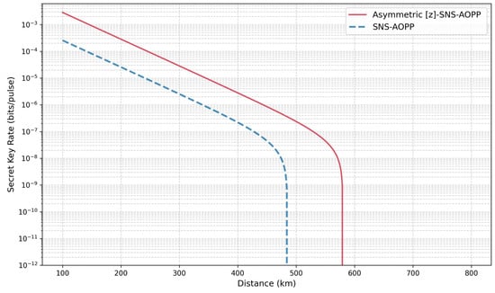
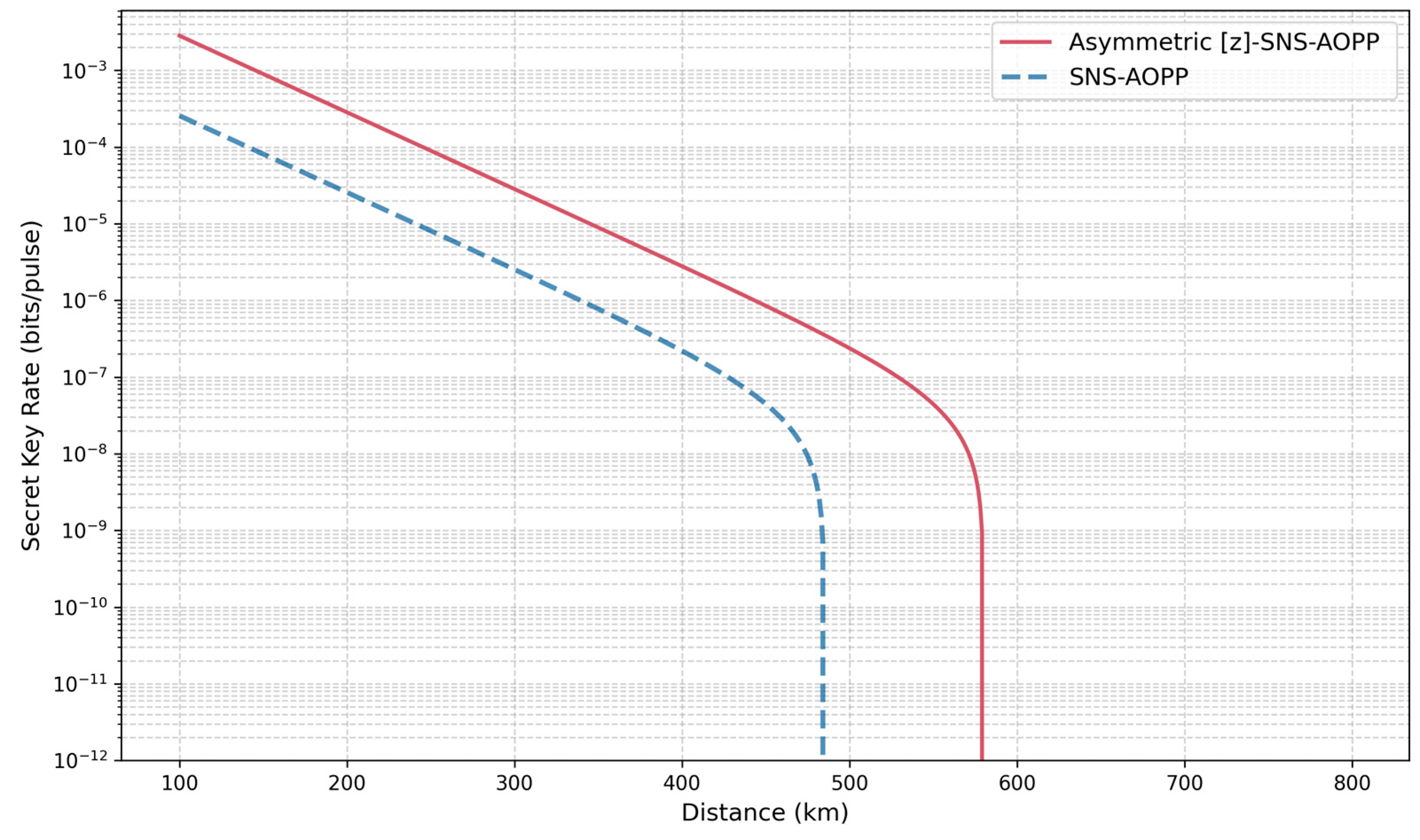
The results obtained and presented in Table 2 demonstrate that the proposed protocol is superior to the SNS protocol with AOPP over the entire distance range, achieving a secret key rate more than 11 times higher, as illustrated in Figure 1.

Table 2. Secret key rates (in bits per pulse) of the simulated protocols.

Distance (km)	Secret Key Rate		Asymmetric [z]-SNS-AOPP vs. SNS-AOPP
	Asymmetric [z]-SNS-AOPP	SNS-AOPP
			Superior Protocol	Ratio
100	2.83 × 10−3	2.56 × 10−4	Asymmetric [z]-SNS-AOPP	11.1
200	2.83 × 10−4	2.56 × 10−5	Asymmetric [z]-SNS-AOPP	11.1
300	2.82 × 10−5	2.52 × 10−6	Asymmetric [z]-SNS-AOPP	11.2
400	2.78 × 10−6	2.19 × 10−7	Asymmetric [z]-SNS-AOPP	12.7
485	3.53 × 10−7	0.0	Asymmetric [z]-SNS-AOPP	-

Figure 1. Secret key rate vs. transmission distance (km).

The results presented in Table 3 indicate that the Asymmetric [z] SNS-AOPP protocol is more robust and offers superior efficiency compared to SNS-AOPP.

Table 3. Distance (km) at which a given secret key rate can be achieved.

Secret Key Rate	Asymmetric [z]-SNS-PM	SNS-AOPP	Superior Protocol	Gain
1 kbps	443.1	339.4	Asymmetric [z]-SNS-PM	103.7 km
100 bps	528.8	427.2	Asymmetric [z]-SNS-PM	101.6 km
1 bps	579.1	483.5	Asymmetric [z]-SNS-PM	95.6 km
0.1 bps	579.8	484.5	Asymmetric [z]-SNS-PM	95.3 km

At a secret key rate of 100 bps (Table 3), the Asymmetric [z] SNS-AOPP protocol reaches 528.8 km, extending the distance by 101.6 km relative to SNS-AOPP.

The largest distance gain is obtained at a secret key rate of 1 kbps: 103.7 km over SNS-AOPP.

The key rates of the proposed protocol reported in Table 4 are obtained without distance-dependent optimization of p_high and p_low. Even under this non-optimized configuration, the proposed protocol achieves higher key rates than the Universal SNS universal with option [x, y, z] at all tested distances (200–380 km), and the advantage grows with distance.

Table 4. Key rate comparison between the proposed protocol and the Universal SNS with option [x, y, z] (N = 10¹⁰) at various transmission distances.

Protocol	200 km	300 km	350 km	380 km
Asymmetric [z] SNS-AOPP	2.83 × 10−4	2.82 × 10−5	8.90 × 10−6	4.44 × 10−6
Universal SNS with option [x, y, z]	4.76 × 10−5	2.95 × 10−6	4.83 × 10−7	8.12 × 10−8

6. Conclusions

The proposed protocol extends the Universal SNS framework (option [z]) by introducing asymmetric probabilities, which increases the fraction of single-sided events contributing to the raw key. Our work demonstrates that a simple modification, asymmetric sending probabilities, can significantly enhance the performance of SNS-TF-QKD.

The security of the proposed protocol has been demonstrated in the finite-key regime within the composable security framework. The analysis covers all possible bias configurations, with the phase-flip error rate bounded by the worst case over the two subsets.

The proposed protocol can be implemented on existing SNS-TF-QKD setups by simply adjusting the sending probabilities, without requiring changes to the quantum hardware. This makes it a practical and cost-effective enhancement for real-world Quantum Key Distribution systems.

In the present work, the optical intensities are intentionally kept fixed for all considered protocols to ensure a fair and consistent comparison. Although a joint optimization of the sending probabilities and optical intensities may further improve the secret key rate, such an optimization is beyond the scope of this work and will be investigated in future research.

References

- Bennett, C.H.; Brassard, G. Quantum cryptography: Public key distribution and coin tossing. Theor. Comput. Sci. 2014, 560, 7–11. [Google Scholar] [CrossRef] [Scilit]
- Bennett, C.H.; Bessette, F.; Brassard, G.; Salvail, L.; Smolin, J. Experimental quantum cryptography. J. Cryptol. 1992, 5, 3–28. [Google Scholar] [CrossRef] [Scilit]
- Lo, H.K.; Ma, X.; Chen, K. Decoy State Quantum Key Distribution. Phys. Rev. Lett. 2005, 94, 230504. [Google Scholar] [CrossRef] [Scilit] [PubMed]
- Lo, H.K.; Curty, M.; Qi, B. Measurement-Device-Independent Quantum Key Distribution. Phys. Rev. Lett. 2012, 108, 130503. [Google Scholar] [CrossRef] [Scilit] [PubMed]
- Liu, Y.; Chen, T.Y.; Wang, L.J.; Liang, H.; Shentu, G.L.; Wang, J.; Cui, K.; Yin, H.L.; Liu, N.L.; Li, L. Experimental Measurement-Device-Independent Quantum Key Distribution. Phys. Rev. Lett. 2013, 111, 130502. [Google Scholar] [CrossRef] [Scilit] [PubMed]
- Da Silva, T.F.; Vitoreti, D.; Xavier, G.B.; Do Amaral, G.C.; Temporão, G.P.; Von Der Weid, J.P. Proof-of-principle demonstration of measurement-device-independent quantum key distribution using polarization qubits. Phys. Rev. A 2013, 88, 052303. [Google Scholar] [CrossRef] [Scilit]
- Tang, Z.; Liao, Z.; Xu, F.; Qi, B.; Qian, L.; Lo, H.K. Experimental demonstration of polarization-encoding measurement-device-independent quantum key distribution. Phys. Rev. Lett. 2014, 112, 190503. [Google Scholar] [CrossRef] [Scilit] [PubMed]
- Curty, M.; Xu, F.; Cui, W.; Lim, C.C.W.; Tamaki, K.; Lo, H.K. Finite-key analysis for measurement-device-independent quantum key distribution. Nat. Commun. 2014, 5, 3732. [Google Scholar] [CrossRef] [Scilit] [PubMed]
- Xu, F.; Xu, H.; Lo, H.-K. Protocol choice and parameter optimization in decoy-state measurement-device-independent quantum key distribution. Phys. Rev. A 2014, 89, 052333. [Google Scholar] [CrossRef] [Scilit]
- Lucamarini, M.; Yuan, Z.L.; Dynes, J.F.; Shields, A.J. Overcoming the rate–distance limit of quantum key distribution without quantum repeaters. Nature 2018, 557, 400–403. [Google Scholar] [CrossRef] [Scilit] [PubMed]
- Wang, X.B.; Yu, Z.W.; Hu, X.L. Twin-field quantum key distribution with large misalignment error. Phys. Rev. A 2018, 98, 062323. [Google Scholar] [CrossRef] [Scilit]
- Ma, X.; Zeng, P.; Zhou, H. Phase-Matching quantum key distribution. Phys. Rev. X 2018, 8, 031043. [Google Scholar] [CrossRef] [Scilit]
- Liu, Y.; Zhang, W.J.; Jiang, C.; Chen, J.P.; Zhang, C.; Pan, W.X.; Ma, D.; Dong, H.; Xiong, J.M.; Zhang, C.J.; et al. Experimental Twin-Field Quantum Key Distribution over 1000 km Fiber. Phys. Rev. Lett. 2023, 130, 210801. [Google Scholar] [CrossRef] [Scilit] [PubMed]
- Pirandola, S.; Laurenza, R.; Ottaviani, C.; Banchi, L. Fundamental limits of repeaterless quantum communications. Nat. Commun. 2017, 8, 15043. [Google Scholar] [CrossRef] [Scilit] [PubMed]
- Tamaki, K.; Lo, H.-K.; Wang, W.; Lucamarini, M. Information theoretic security of quantum key distribution overcoming the repeaterless secret key capacity bound. arXiv 2018, arXiv:1805.05511. [Google Scholar]
- Cui, C.; Yin, Z.-Q.; Wang, R.; Chen, W.; Wang, S.; Guo, G.-C.; Han, Z.-F. Twin-Field Quantum Key Distribution without Phase Postselection. Phys. Rev. Appl. 2019, 11, 034053. [Google Scholar] [CrossRef] [Scilit]
- Curty, M.; Azuma, K.; Lo, H.-K. Simple security proof of twin-field type quantum key distribution protocol. npj Quantum Inf. 2019, 5, 64. [Google Scholar] [CrossRef] [Scilit]
- Lu, F.Y.; Yin, Z.Q.; Cui, C.H.; Fan-Yuan, G.J.; Wang, R.; Wang, S.; Chen, W.; He, D.Y.; Huang, W.; Xu, B.J.; et al. Improving the performance of Twin-Field Quantum Key Distribution. Phys. Rev. A 2019, 100, 022306. [Google Scholar] [CrossRef] [Scilit]
- Currás-Lorenzo, G.; Navarrete, Á.; Azuma, K.; Kato, G.; Curty, M.; Razavi, M. Tight finite-key security for twin-field quantum key distribution. npj Quantum Inf. 2021, 7, 22. [Google Scholar] [CrossRef] [Scilit]
- Maeda, K.; Sasaki, T.; Koashi, M. Repeaterless quantum key distribution with efficient finite-key analysis overcoming the rate-distance limit. Nat. Commun. 2019, 10, 3140. [Google Scholar] [CrossRef] [Scilit] [PubMed]
- Minder, M.; Pittaluga, M.; Roberts, G.L.; Lucamarini, M.; Dynes, J.F.; Yuan, Z.L.; Shields, A.J. Experimental quantum key distribution beyond the repeaterless secret key capacity. Nat. Photon. 2019, 13, 334–338. [Google Scholar] [CrossRef] [Scilit]
- Liu, Y.; Yu, Z.W.; Zhang, W.; Guan, J.Y.; Chen, J.P.; Zhang, C.; Hu, X.L.; Li, H.; Jiang, C.; Lin, J.; et al. Experimental Twin-Field Quantum Key Distribution through Sending or. Not. Sending. Phys. Rev. Lett. 2019, 123, 100505. [Google Scholar] [CrossRef] [Scilit] [PubMed]
- Wang, S.; He, D.-Y.; Yin, Z.-Q.; Lu, F.-Y.; Cui, C.-H.; Chen, W.; Zhou, Z.; Guo, G.-C.; Han, Z.-F. Beating the Fundamental Rate-Distance Limit in a Proof-of-Principle Quantum Key Distribution System. Phys. Rev. X 2019, 9, 021046. [Google Scholar] [CrossRef] [Scilit]
- Zhong, X.; Hu, J.; Curty, M.; Qian, L.; Lo, H.-K. Proof-of-Principle Experimental Demonstration of Twin-Field Type Quantum Key Distribution. Phys. Rev. Lett. 2019, 123, 100506. [Google Scholar] [CrossRef] [Scilit] [PubMed]
- Chen, J.P.; Zhang, C.; Liu, Y.; Jiang, C.; Zhang, W.; Hu, X.L.; Guan, J.Y.; Yu, Z.W.; Xu, H.; Lin, J.; et al. Sending-or-Not-Sending with Independent Lasers: Secure Twin-Field Quantum Key Distribution over 509 km. Phys. Rev. Lett. 2020, 124, 070501. [Google Scholar] [CrossRef] [Scilit] [PubMed]
- Liu, H.; Jiang, C.; Zhu, H.T.; Zou, M.; Yu, Z.W.; Hu, X.L.; Xu, H.; Ma, S.; Han, Z.; Chen, J.P.; et al. Field Test of Twin-Field Quantum Key Distribution through Sending-or-Not-Sending over 428 km. Phys. Rev. Lett. 2021, 126, 250502. [Google Scholar] [CrossRef] [Scilit] [PubMed]
- Chen, J.P.; Zhang, C.; Liu, Y.; Jiang, C.; Zhang, W.J.; Han, Z.Y.; Ma, S.Z.; Hu, X.L.; Li, Y.H.; Liu, H.; et al. Twin-Field Quantum Key Distribution over 511 km Optical Fiber Linking two Distant Metropolitans. Nat. Photon. 2021, 15, 570. [Google Scholar] [CrossRef] [Scilit]
- Pittaluga, M.; Minder, M.; Lucamarini, M.; Sanzaro, M.; Woodward, R.I.; Li, M.-J.; Yuan, Z.; Shields, A.J. 600 km repeater-like quantum communications with dual-band stabilization. Nat. Photon. 2021, 15, 530–535. [Google Scholar] [CrossRef] [Scilit]
- Wang, Z.H.; Wang, R.; Yin, Z.Q.; Wang, S.; Lu, F.Y.; Chen, W.; He, D.Y.; Guo, G.C.; Han, Z.F. Tight finite-key analysis for mode-pairing quantum key distribution. Nat. Photon. 2022, 16, 154–161. [Google Scholar]
- Clivati, C.; Meda, A.; Donadello, S.; Virzì, S.; Genovese, M.; Levi, F.; Mura, A.; Pittaluga, M.; Yuan, Z.; Shields, A.J.; et al. Coherent phase transfer for real-world twin-field quantum key distribution. Nat. Commun. 2022, 13, 157. [Google Scholar] [CrossRef] [Scilit] [PubMed]
- Yu, Z.W.; Hu, X.L.; Jiang, C.; Xu, H.; Wang, X.B. Sending-or-not-sending twin-field quantum key distribution in practice. Sci. Rep. 2019, 9, 3080. [Google Scholar] [CrossRef] [Scilit] [PubMed]
- Jiang, C.; Yu, Z.-W.; Hu, X.-L.; Wang, X.-B. Unconditional security of sending or not sending twin-field quantum key distribution with finite pulses. Phys. Rev. Appl. 2019, 12, 024061. [Google Scholar] [CrossRef] [Scilit]
- Hu, X.-L.; Jiang, C.; Yu, Z.-W.; Wang, X.-B. Sending-or-not-sending twin-field protocol for quantum key distribution with asymmetric source parameters. Phys. Rev. A 2019, 100, 062337. [Google Scholar] [CrossRef] [Scilit]
- Xu, H.; Yu, Z.-W.; Jiang, C.; Hu, X.-L.; Wang, X.-B. Sending-or-not-sending twin-field quantum key distribution: Breaking the direct transmission key rate. Phys. Rev. A 2020, 101, 042330. [Google Scholar] [CrossRef] [Scilit]
- Jiang, C.; Hu, X.L.; Xu, H.; Yu, Z.W.; Wang, X.B. Zigzag approach to higher key rate of sending-or-not-sending twin field quantum key distribution with finite-key effects. New J. Phys. 2020, 22, 053048. [Google Scholar] [CrossRef] [Scilit]
- Jiang, C.; Hu, X.-L.; Yu, Z.-W.; Wang, X.-B. Composable security for practical quantum key distribution with two way classical communication. New J. Phys. 2021, 23, 063038. [Google Scholar] [CrossRef] [Scilit]
- Teng, J.; Yin, Z.Q.; Fan-Yuan, G.J.; Lu, F.Y.; Wang, R.; Wang, S.; Chen, W.; Huang, W.; Xu, B.J.; Guo, G.C.; et al. Sending-or-not-sending twin-field quantum key distribution with multiphoton states. Phys. Rev. A 2021, 104, 062441. [Google Scholar] [CrossRef] [Scilit]
- Chernoff, H. A Measure of Asymptotic Efficiency for Tests of a Hypothesis Based on the sum of Observations. Ann. Math. Stat. 1952, 23, 493. [Google Scholar] [CrossRef] [Scilit]
- Huang, J.; Li, W.; Qiao, Y. An Effective Parameter Analysis for Sending-or-Not-Sending Quantum Key Distribution with Untrusted Light. Entropy 2025, 27, 547. [Google Scholar] [CrossRef] [Scilit] [PubMed]
- Shan, Y.G.; Zhou, Y.; Yin, Z.Q.; Wang, S.; Chen, W.; He, D.Y.; Guo, G.C.; Han, Z.F. Sending-or-not-sending quantum key distribution with phase postselection. Phys. Rev. Appl. 2024, 22, 024056. [Google Scholar] [CrossRef] [Scilit]
- Hu, X.L.; Jiang, C.; Yu, Z.W.; Wang, X.B. Universal approach to sending-or-not-sending twin field quantum key distribution. Quantum Sci. Technol. 2022, 7, 045031. [Google Scholar] [CrossRef] [Scilit]
- Tomamichel, M.; Lim, C.C.W.; Gisin, N.; Renner, R. Tight Finite-Key Analysis for Quantum Cryptography. Nat. Commun. 2012, 3, 634. [Google Scholar] [CrossRef] [Scilit] [PubMed]
Disclaimer/Publisher’s Note: The statements, opinions and data contained in all publications are solely those of the individual author(s) and contributor(s) and not of MDPI and/or the editor(s). MDPI and/or the editor(s) disclaim responsibility for any injury to people or property resulting from any ideas, methods, instructions or products referred to in the content. |
© 2026 by the authors. Licensee MDPI, Basel, Switzerland. This article is an open access article distributed under the terms and conditions of the Creative Commons Attribution (CC BY) license.