


Abstract
Multi-label text feature selection aims to identify compact and discriminative feature subsets for documents associated with multiple correlated labels. In federated environments, this task is further complicated by high-dimensional search spaces, non-independent and non-identically distributed data, complex label dependencies, and the requirement that raw feature and label data remain local. To address these challenges, this paper proposes the Federated Anchor-Guided Frequency-Domain Optimization Algorithm (Fed-AGFDO), a federated multi-label text feature selection framework. At each client, the Anchor-Guided Frequency-Domain Optimization (AGFDO) module transforms the encoded search population into the frequency domain and combines random spectral exploration, elite-guided mixing, diversity-aware anchor screening, and multi-anchor direction aggregation to balance exploration and exploitation. Candidate feature-weight vectors are evaluated using a manifold-regularized fitness function that jointly considers sample structure, label-consensus regularization, sparsity regularization, and a soft global feature-weight consistency penalty. The server aggregates only local feature-weight vectors through sample-size-weighted aggregation followed by an exponential moving average update to smooth inter-round changes in the global feature weights while keeping raw data local. Experiments on eight multi-label text datasets demonstrate that Fed-AGFDO achieves strong classification and label-ranking performance with compact feature subsets. Under the representative subset settings, Fed-AGFDO improves Average Precision by up to over Fuzzy Federated Multi-Label Feature Selection (Fuzzy FMFS) and reduces Ranking Loss by up to relative to Federated Multi-Label Feature Selection (FMLFS). Parameter sensitivity and ablation analyses further demonstrate robustness across the examined parameter ranges and the complementary contributions of anchor guidance, diversity screening, and multi-anchor aggregation. These results indicate that Fed-AGFDO provides an effective and data-locality-aware solution for high-dimensional federated multi-label text feature selection.
1. Introduction
In recent years, the rapid development of the internet, smart healthcare, and digital media platforms has led to a continuous increase in the volume of text data. An increasing number of real-world tasks require the simultaneous prediction of multiple semantic categories associated with a single document, making multi-label text classification an important research topic in natural language processing. Unlike conventional single-label classification, multi-label text data are typically high-dimensional, sparse, and highly redundant. Moreover, complex correlations, co-occurrence relationships, and latent semantic dependencies among labels further complicate model training [1]. As the dimensionality of text representations increases, a large number of irrelevant or weakly informative features may exacerbate the curse of dimensionality and increase computational and storage costs. They may also lead to model overfitting and impair the generalization capability of classification models [2]. Therefore, selecting a compact subset of highly discriminative features from a large number of candidate text features, while reducing computational complexity and preserving multi-label classification performance, has become an important research problem in multi-label text analysis.
However, in practical applications, text data are often distributed across different institutions, organizations, or end devices. Data governance policies, confidentiality requirements, and restrictions on data exchange may prevent these data from being centralized on a single server. In such scenarios, the motivation for federated learning (FL) is determined primarily by distributed data ownership and data-locality constraints rather than by the absolute size of an individual local dataset. Even when each participating party holds a moderate amount of data, centralized feature selection may still be infeasible when raw data cannot be directly pooled or exchanged. Federated learning therefore provides a suitable framework for collaborative data analysis by allowing multiple parties to exchange model parameters or intermediate information while keeping their raw data local [3]. Nevertheless, extending feature selection to federated multi-label text settings remains challenging. On the one hand, data that are not independently and identically distributed (Non-IID) are common across clients. Different clients may have distinct distributions of text topics, label preferences, and statistical patterns of features. These differences may result in substantial discrepancies in local feature importance evaluation [4,5]. On the other hand, the sparse and high-dimensional representations of multi-label text, together with complex label dependencies, further enlarge the feature search space. In addition, communication constraints and privacy requirements in federated environments require an algorithm to have both strong local search capability and the ability to effectively use collaborative information from multiple clients [6]. Therefore, achieving stable and efficient federated multi-label text feature selection without sharing raw text data remains a challenging research problem.
Although continuous progress has been made in both multi-label feature selection and federated feature selection, their integration still presents several limitations. First, most multi-label text feature selection methods assume centralized data access and require the complete training dataset for feature evaluation or optimization. Consequently, these methods cannot be directly transferred to federated environments when data cannot be centrally stored because of privacy constraints. Second, existing federated feature selection methods generally rely on statistical evaluation criteria, models with structural constraints, or conventional optimization strategies [7,8]. Although these methods can integrate feature-importance information across clients to a certain extent, sparse and high-dimensional text representations remain challenging because of the enlarged search space and heterogeneous local evaluations. For optimization-driven approaches in particular, candidate evolution is still mainly performed in the original solution space, leaving alternative transformed search representations relatively underexplored [9].
In recent years, frequency-domain analysis has provided an alternative representation for complex optimization problems. Unlike methods that update candidate solutions directly in the original variable space, frequency-domain methods map candidate solutions into transformed coordinates through the Fourier Transform and perform search operations in this alternative representation, providing a new perspective for exploration during optimization [10]. Candidate solutions in high-dimensional feature selection can generally be represented as continuous or discrete vectors of feature weights. Such vectors can be transformed into frequency-domain representations using the Discrete Fourier Transform (DFT) or its efficient implementation, the Fast Fourier Transform (FFT), without changing the dimensionality of the search space. Since each transformed coefficient depends on the complete candidate vector, perturbations applied in the transformed coordinates can be mapped through the inverse transform into coordinated adjustments across multiple original dimensions. This use of the Fourier transform does not require neighboring feature indices to possess spatial, temporal, or semantic locality, but instead provides an alternative global representation for the optimization process. Existing studies have shown that frequency-domain representations can provide search behaviors for continuous optimization that differ from conventional operations in the original solution space. However, existing frequency-domain optimization methods are mainly designed for general continuous optimization problems. Their application to federated multi-label text feature selection, where high-dimensional feature search, client heterogeneity, label dependencies, and data-locality constraints need to be considered jointly, remains insufficiently investigated.
To address these issues, this study proposes the Federated Anchor-Guided Frequency-Domain Optimization Algorithm (Fed-AGFDO) for federated multi-label text feature selection. Fed-AGFDO introduces an anchor-guided frequency-domain optimization mechanism into the FL framework and enables collaborative feature search across clients without sharing raw text data. Specifically, on the client side, Anchor-Guided Frequency-Domain Optimization (AGFDO) is designed as the local optimizer. AGFDO maintains a set of elite anchors selected from high-quality candidate solutions while ensuring sufficient diversity among them. The directional information provided by these anchors is then used to guide spectral updates, thereby providing directional guidance for balancing exploration and exploitation in sparse, high-dimensional text space. Meanwhile, a structured feature evaluation mechanism is used to assess the quality of candidate solutions. Manifold constraints and sparsity regularization are incorporated into the optimization objective to preserve local data structures and encourage sparse global feature importance during feature selection. They improve the reliability of feature weight estimation, whereas the actual search process is driven by the frequency-domain optimization mechanism of AGFDO. On the server side, a federated aggregation mechanism for feature weights is designed to support knowledge sharing among clients. It combines aggregation weighted by client sample size with smooth updates across communication rounds, thereby improving global feature selection without exchanging raw text data. Based on these designs, Fed-AGFDO enables effective multi-label text feature selection while keeping data local. The main contributions of this study are summarized as follows:
- A federated multi-label text feature selection framework, Fed-AGFDO, is proposed. It integrates frequency-domain optimization at the clients with collaborative aggregation at the server. This framework enables the collaborative optimization of feature weights across clients without sharing raw text data and provides a data-locality-aware solution for federated multi-label text feature selection.
- An anchor-guided frequency-domain optimization method, AGFDO, is developed. By introducing diverse elite anchors and a spectral update strategy guided by these anchors, AGFDO provides more effective search directions in sparse, high-dimensional text space. It therefore supports a more effective balance between exploration and exploitation during the optimization process.
- A federated aggregation strategy for feature weights is designed. This strategy exchanges only feature-weight vectors between the clients and the server and combines sample-size-weighted aggregation with exponential moving average (EMA) updating. The EMA step smooths inter-round changes in the aggregated feature weights while incorporating information from the current client updates.
- Systematic experiments are conducted on eight publicly available multi-label text datasets under a unified evaluation protocol. Comparative, sensitivity, ablation and controlled, federated robustness, statistical, and practical-efficiency analyses are performed to evaluate the effectiveness, robustness, and practical characteristics of the proposed framework.
The remainder of this paper is organized as follows. Section 2 reviews related studies on multi-label text feature selection, metaheuristic optimization, frequency-domain optimization, and federated feature selection. Section 3 presents the formulation of federated multi-label text feature selection, together with the Fed-AGFDO framework and its optimization procedure. Section 4 reports the experimental setup, comparative results, sensitivity and controlled analyses, federated robustness, statistical significance, and practical efficiency. Finally, Section 5 concludes the paper and discusses future research directions.
2. Related Work
This section reviews the literature related to Fed-AGFDO from three perspectives: multi-label text feature selection, metaheuristic and frequency-domain optimization, and federated feature selection. Based on these research directions, the limitations of existing methods are summarized to motivate the development of frequency-domain collaborative feature selection for high-dimensional and heterogeneous federated text data.
2.1. Multi-Label Text Feature Selection
Multi-label text feature selection (MLTFS) aims to identify a compact and highly discriminative subset of features from high-dimensional text representations. Its goal is to reduce data dimensionality and computational cost while preserving multi-label classification performance. Text data are typically high-dimensional, sparse, and highly redundant, while each sample in a multi-label task may be associated with multiple semantic labels. Therefore, feature selection must consider not only the importance of individual features but also the relationships between features and multiple labels, as well as the latent dependencies among labels [11].
Existing MLTFS methods can generally be divided into three categories: statistical evaluation methods, structural representation methods, and optimization-driven methods.
Statistical evaluation methods generally rank candidate features by analyzing the relationships between features and labels [12,13]. These methods commonly measure feature contributions using information-theoretic criteria, statistical correlations, or probabilistic analysis [14,15]. They may also use strategies for controlling redundancy to select features with high information content [16]. Owing to their relatively low computational cost, these methods have been widely used for processing large-scale text data [17]. However, methods based on manually designed evaluation criteria often fail to fully capture complex label dependencies and nonlinear semantic relationships [18]. They therefore remain limited when dealing with the high-order label structures commonly found in multi-label text data.
To improve the modeling of intrinsic data structures, structural representation methods have gradually been introduced into multi-label feature selection. These methods construct structural constraints or representations in a latent space [19,20,21]. In this way, they jointly consider sample relationships, label dependencies, and feature structures [22]. Common techniques include sparse learning, low-rank representation, and manifold learning. These techniques can exploit the intrinsic structure of the data and improve the compactness of feature representations [23,24,25,26,27,28]. However, such methods generally depend on predefined structural constraints or continuous optimization procedures. Therefore, they have limited ability to address search problems that involve complex combinations of discrete features.
Optimization-driven methods formulate feature selection as a combinatorial optimization problem [29]. They use search strategies to directly identify feature subsets that satisfy the requirements for classification performance. Compared with methods based on fixed evaluation criteria, these approaches can balance classification performance against the size of the selected feature subset [30]. They therefore offer greater flexibility. Nevertheless, in high-dimensional text space, conventional optimization-driven methods remain prone to rapid expansion of the search space and convergence to local optima.
Overall, existing MLTFS studies have established a relatively comprehensive methodological framework. However, most methods are still developed under the assumption of centralized data access and require the complete training dataset for feature evaluation or search. When text data are distributed across multiple clients and cannot be centralized, effective feature selection without accessing raw data remains an important topic for further investigation.
2.2. Metaheuristic Optimization and Frequency-Domain Search
Feature selection is inherently a combinatorial optimization problem. Consequently, metaheuristic methods have been widely used to search for feature subsets in high-dimensional data [31,32]. Unlike feature ranking methods that rely on a single evaluation criterion, metaheuristic algorithms simulate search mechanisms observed in natural systems to identify near-optimal solutions in complex search space. In recent years, particle swarm optimization [33], genetic algorithms [34], differential evolution [35], ant colony optimization [36], and other methods based on swarm intelligence have been widely applied to feature selection, classification optimization, and combinatorial decision tasks [37,38].
To improve search performance, numerous strategies have been proposed, including adaptive parameter adjustment [39], hybrid search mechanisms [40,41,42], multi-objective optimization [43,44], and cooperative coevolution [45]. These strategies can improve the exploration capability and stability of the search process. However, most conventional metaheuristic algorithms still operate directly in the original solution space. Their optimization procedures mainly rely on position updates among candidate solutions, random perturbations, and neighborhood search. In sparse, high-dimensional text space, the number of search dimensions increases rapidly. Limited search resources may therefore be insufficient to cover the entire solution space [46], which can result in reduced search efficiency and premature convergence.
In recent years, frequency-domain analysis has been explored as an alternative representation for optimization. The Fourier Transform maps a candidate vector from its original coordinates to a set of globally coupled transformed coefficients. Since each Fourier coefficient depends on the complete input vector, search operations performed in the transformed coordinates can induce coordinated changes across multiple original dimensions after inverse transformation. This representation has therefore been investigated as an alternative to direct updates in the original solution space [10].
For feature selection, a candidate solution can generally be represented as a feature-weight vector or a binary selection sequence. Such a vector can be algebraically transformed using DFT/FFT without assuming spatial, temporal, or semantic adjacency among feature indices. Related studies have investigated search operations in these transformed coordinates and then mapped the updated candidates back to the original space [10]. This provides an alternative representation for balancing exploration and exploitation in continuous optimization.
However, existing frequency-domain optimization methods mainly address general continuous optimization problems. Their design objectives differ substantially from those of federated MLTFS. On the one hand, MLTFS requires the encoding of discrete feature subsets and complex evaluation based on classification performance. On the other hand, federated environments introduce additional challenges, including client heterogeneity, communication constraints, and privacy requirements. Therefore, how to integrate frequency-domain search with federated MLTFS and use effective guidance to improve search performance in high-dimensional space remains insufficiently studied.
2.3. Federated Feature Selection
As the demand for data privacy continues to increase, FL has provided a new solution for collaborative data analysis in distributed environments. It has also promoted the development of federated feature selection. Unlike conventional centralized feature selection, federated feature selection cannot directly access the raw data of all clients. It therefore relies on collaboration among clients to estimate global feature importance and optimize feature selection without centralizing raw data [47].
Existing studies on federated feature selection mainly follow two research directions. The first direction focuses on computing local feature importance at each client and obtaining a global evaluation through aggregation at the server [7]. These methods generally measure feature value using statistical correlations, information content, or model contributions. Their main advantages are relatively low communication costs and ease of deployment. However, data distributions often differ across clients, which may introduce bias into local evaluation results. As a result, simple aggregation may fail to accurately reflect the global importance of each feature [48].
The second direction extends conventional feature selection models to federated environments and exploits complementary information across clients through joint optimization. Structural constraints and sparse regularization are commonly used to improve the estimation of feature weights [9]. For example, manifold constraints can characterize structures in the sample and label spaces, while the -norm can induce row sparsity in the feature-weight matrix. However, these constraints mainly improve the reliability of feature evaluation rather than directly addressing the search for discrete feature combinations in high-dimensional space.
To improve the search for complex feature combinations in federated environments, several studies have introduced population-based optimization into federated feature selection [8,49]. Recent work has further explored this direction in federated multi-label feature selection. Zheng et al. [50] combined manifold-aware sparse modeling with cooperative grey wolf optimization in a two-stage client-side framework, while the dual-layer hybrid breeding cooperative particle swarm optimization method [51] integrated manifold and sparsity regularization with population-based collaborative search. These studies demonstrate the effectiveness of combining structural feature evaluation with evolutionary optimization in federated multi-label settings. In contrast, the present work focuses on a different search representation and guidance mechanism: the encoded population is evolved in Fourier-transformed coordinates, and diversity-aware multi-anchor guidance is introduced to direct the spectral search.
Therefore, further improvement in federated MLTFS requires search mechanisms that can complement existing structural modeling and population-based optimization with alternative solution representations and more informative directional guidance. Such mechanisms may provide additional flexibility for exploring high-dimensional feature spaces while retaining federated collaboration.
2.4. Summary and Research Gap
In summary, extensive studies have investigated MLTFS, metaheuristic optimization, and federated feature selection. Nevertheless, a clear research gap remains at the intersection of these three areas.
First, most existing MLTFS methods assume centralized data availability and require access to the complete training dataset for feature evaluation and optimization. Consequently, they are difficult to apply directly to distributed text environments in which data cannot be centralized because of privacy constraints.
Second, recent federated multi-label feature-selection methods have increasingly incorporated structural regularization and population-based optimization to improve feature evaluation and search. However, their candidate evolution is still mainly performed in the original solution space. In sparse and high-dimensional text representations, alternative search representations together with diversity-aware directional guidance remain insufficiently explored.
Finally, frequency-domain optimization provides an alternative representation for population-based search, but its integration with federated MLTFS remains insufficiently investigated. In particular, how to combine spectral search with diversity-aware directional guidance and federated feature-weight coordination has received limited attention.
Based on these observations, a federated feature-selection method that combines an alternative search representation with diversity-aware guidance provides a natural direction for improving high-dimensional collaborative optimization.
3. The Proposed Method
This section presents Fed-AGFDO for federated MLTFS. It first formulates the optimization problem and introduces the overall framework, and then describes the client-side anchor-guided frequency-domain search, manifold-regularized fitness evaluation, federated feature-weight aggregation and updating, global feature ranking and subset construction, and computational and communication complexity.
3.1. Federated Multi-Label Text Feature Selection Formulation
As the volume of text data continues to increase, multi-label text classification requires discriminative feature subsets to be learned from high-dimensional text representations. In practical applications, however, text data are often generated independently by different entities and cannot be directly centralized because of data governance policies and privacy requirements. This study therefore considers MLTFS in an FL setting. The objective is to obtain discriminative global feature weights through collaborative optimization across clients without sharing raw text data and to use these weights to generate a compact feature subset for multi-label classification.
Let the multi-label text dataset used for federated training be denoted by , where is the total number of training samples, is the d-dimensional feature vector of the i-th text sample, and is the corresponding multi-label vector. The number of labels is denoted by L. The feature matrix and label matrix formed by all training samples are, respectively, written as and .
In the FL setting, the training data are distributed across C clients. Client c holds the local dataset , where , , , and is the number of local training samples at client c. The local sample sizes satisfy .
All clients share the same feature and label spaces, but their sample sizes and label distributions may differ. This study considers a horizontal FL setting with Non-IID data. For any two distinct clients c and , their local joint distributions generally satisfy for . This heterogeneity is mainly reflected in imbalanced client sample sizes and shifts in label proportions.
The objective of federated MLTFS is to learn a continuous feature-weight vector without centralizing the data held by the clients. The feature-weight vector is defined as
As defined in Equation (1), assigns a continuous importance score to each of the d features, where represents the importance of the j-th feature. A larger value of indicates a greater contribution of the corresponding feature to multi-label classification. After federated optimization, the server ranks all features according to the final global weights and selects the features with the highest weights to form the final subset. The detailed mapping procedure is provided in Section 3.6.1.
For client c, the base local fitness of a candidate feature-weight vector is defined in Equation (2):
where is the feature–label weight matrix constructed from the shared feature-weight vector , is the latent label representation at client c, and is a proxy objective constructed from the local data structure and shared feature importance. Specifically, , where denotes an all-one vector with length L. Therefore, all labels share the same feature-weight representation, and the model learns global feature importance rather than label-specific feature weights.
During federated round r, the actual fitness function used by client c is denoted by . When no global weights are available, is equal to the base local fitness . When the global weights obtained from the previous round are available, the fitness also includes a soft global consistency penalty. The proxy objective, base fitness, and global consistency penalty are defined in Section 3.4.
From a system-level perspective, the round-specific federated objective can be conceptually characterized as
where reflects the relative contribution of client c according to its local sample size. Equation (3) provides a system-level characterization of the aggregate optimization objective across clients and establishes the relationship between the local round-specific objectives and the overall federated optimization goal. It does not correspond to a centralized objective that is explicitly evaluated or directly minimized by the server. Instead, during communication round r, each client independently optimizes using only its local data and obtains a locally optimized feature-weight vector. The server receives these local feature-weight vectors rather than local objective values or gradients, and coordinates them through the sample-size-weighted aggregation and EMA-based global updating described in Section 3.5. Accordingly, the practical realization of Fed-AGFDO relies on distributed local optimization and server-side feature-weight aggregation, while serves as a conceptual system-level formulation of the collaborative optimization objective.
3.2. Federated Optimization Workflow
To address feature selection for high-dimensional multi-label text in an FL setting, this study proposes Fed-AGFDO. The method consists of the local AGFDO optimizer deployed at each client and a feature-weight aggregation module at the server. A global feature-importance ranking is obtained through multiple rounds of local search and coordinated server updates. Unlike centralized methods, Fed-AGFDO does not collect the complete training dataset. Instead, the clients and the server exchange continuous feature-weight vectors defined in a shared feature space.
As shown in Figure 1, the overall procedure of Fed-AGFDO consists of four stages: client initialization and local optimization, client weight uploading, server aggregation, and global feature selection.
Figure 1.
Overall framework of Fed-AGFDO. The numbered markers 1–4 denote client initialization and local optimization, client weight uploading, server aggregation, and global feature selection, respectively. Blue upward arrows indicate uploaded local feature weights, whereas orange downward arrows indicate global feature weights returned by the server.
- Client initialization and local optimization. During communication round r, the server provides the currently available global feature-weight vector to the clients. In the first round, no historical global weights are available, and each client initializes its search directly from its local data. Client c independently performs AGFDO optimization using the local dataset . Candidate encoding and decoding, frequency-domain search, anchor guidance, and fitness evaluation are then performed to obtain the final retained local feature-weight vector for the current round.
- Client weight uploading. After local optimization, each client uploads its complete continuous feature-weight vector . The local feature matrix , label matrix , local population, anchor information, and spectral coefficients remain at the client and are not transmitted. Therefore, the server receives only the local feature-importance estimates learned by the clients in the shared feature space.
- Server aggregation. After receiving the local feature-weight vectors, the server first performs sample-size-weighted aggregation to obtain the aggregated feature-weight vector for the current communication round. It then updates the global feature weights using an EMA to reduce round-to-round fluctuations caused by Non-IID data and stochastic local search. The updated global feature-weight vector is subsequently provided to the clients as a global reference for the next communication round.
- Global feature selection. After the predefined number of communication rounds has been completed, the server ranks all text features in descending order according to the final global feature weights. The Top-k features are then selected to form the final feature subset for subsequent multi-label classification.
Throughout the federated optimization process, the local feature and label data remain at the clients, while only local and global feature-weight vectors are exchanged between the clients and the server. Fed-AGFDO therefore follows a data-locality-aware federated design in which raw feature and label data are not directly transmitted. This data-locality property does not constitute a formal differential-privacy guarantee for the exchanged feature-weight vectors.
3.3. Anchor-Guided Frequency-Domain Search
This subsection presents the client-side search procedure of AGFDO. It first describes the continuous population representation, structure-aware initialization, feature-weight decoding, and local candidate selection, and then introduces the frequency-domain population update and the anchor-guided spectral mechanism for balancing exploration and exploitation.
3.3.1. Population Initialization and Feature-Weight Decoding
Text representations in federated MLTFS are typically high-dimensional and sparse. Directly searching for discrete feature combinations causes the search space to grow exponentially with the number of features. To reduce the complexity of this combinatorial search, Fed-AGFDO employs continuous search variables and decodes them into continuous feature weights, thereby formulating feature selection as a continuous optimization problem.
(1) Search-space encoding. During federated round r, client c performs AGFDO optimization and maintains a continuous search population. The initial encoded population is defined in Equation (4):
where N is the population size, and denotes the i-th search vector, with . Its j-th element, , is an internal search variable associated with the j-th feature, where . The same encoding is used at subsequent generations, with and denoting the population and the i-th search vector at generation t, respectively. When the initial structure scores are available, controls the direction and magnitude of the residual adjustment applied to the corresponding initial score. When the initial structure scores are unavailable, it directly represents the weight of the corresponding feature. This continuous representation also preserves the numerical information required for subsequent frequency-domain updates.
(2) Initial structural reference. At the beginning of each federated round, client c computes an initial structure score vector from its local data. This vector is defined in Equation (5):
where denotes the initial structure score vector computed by client c, and is the initial score assigned to the j-th feature. A larger value indicates that the corresponding feature is considered more important according to the local sample and label structures. For clarity, the federated-round superscript of is omitted in this subsection.
The score vector is generated using a lightweight structure-aware procedure adapted from manifold-regularized discriminative feature selection [28]. Based on the local graph/fitness subset, the sample Laplacian , label Laplacian , and centering matrix are first constructed. An auxiliary feature–label matrix is randomly initialized and refined for 15 iterations. At each iteration, the latent representation is obtained by solving the Sylvester equation with , , and . A diagonal reweighting matrix is then constructed with , where denotes the double-precision machine epsilon used for numerical stabilization, and is updated as . After 15 iterations, is used as the importance score of feature j, and the resulting vector is min–max normalized to to obtain . The initial structure score remains fixed during the subsequent local AGFDO search and serves as the structural baseline for feature-weight decoding.
(3) Population initialization and decoding. When the initial structure scores are available, the search vectors are initialized around the neutral search position according to Equation (6):
where is the d-dimensional all-ones vector, is the identity matrix, and truncates each element to . The value 0.5 represents the neutral position because it produces a zero residual adjustment after decoding. Therefore, this neutral-centered initialization causes the decoded initial feature-weight vectors to lie near the initial structure scores while preserving random differences among individuals.
When the initial structure scores are unavailable and no previous global weights are available, all search vectors are initialized uniformly over . When is available, approximately 30% of the population is initialized in its neighborhood by adding Gaussian noise with a standard deviation of 0.1 and clipping the perturbed vectors to , while the remaining individuals are initialized uniformly over . This partial initialization introduces information from the previous global solution while retaining sufficient population diversity.
When is available, each encoded search vector is decoded into a feature-weight vector using the residual mapping defined in Equation (7):
where denotes the decoded feature-weight vector of the i-th individual at generation t, and controls the residual adjustment range. For the j-th feature, the corresponding adjustment is . Consequently, increases the corresponding initial score, decreases it, and leaves it unchanged. The element-wise maximum operation removes negative values, and divides the resulting vector by its maximum element. If the maximum value of the truncated vector is zero, is directly used as the decoded result.
When is unavailable, the search space and the feature-weight space are identical, and thus . The search vector participates in the frequency-domain update, whereas the decoded vector is submitted to the round-specific local fitness function. Its fitness value is denoted by . Therefore, AGFDO updates the encoded search vectors, while candidate quality is evaluated using the decoded feature-weight vectors.
(4) Local candidate selection. After the local AGFDO search, let denote the best decoded feature-weight vector found during round r. When the initial structure scores are available, both and are evaluated using the same round-specific fitness function . The client selects its final local feature-weight vector according to Equation (8):
When the initial structure scores are unavailable, is directly retained as . This final comparison prevents the local search from returning a solution inferior to the initial structure-based candidate under the current round-specific evaluation criterion. Therefore, the initial structure scores serve as a fixed baseline for residual decoding and as an additional candidate in the final local selection. The neutral-centered initialization causes the decoded initial candidates to lie near this structural baseline, whereas iterative optimization is performed in the continuous search space through the frequency-domain search mechanism of AGFDO.
3.3.2. Frequency-Domain Search Update
Direct perturbation in a high-dimensional continuous search space may lead to dispersed search directions and unstable updates. AGFDO therefore applies the FFT along the feature dimension to obtain a complex frequency-domain representation of the encoded population. Random spectral exploration, anchor guidance, and elite-guided mixing are then performed, after which the updated spectra are mapped back to the encoded search space using the Inverse Fast Fourier Transform (IFFT).
The frequency-domain transformation does not change the dimensionality of the encoded search space. It provides an alternative numerical representation for search updates, while the updated vectors are mapped back through the inverse transform before decoding and fitness evaluation. Therefore, the Fourier representation does not redefine the semantics of individual text features or require neighboring feature indices to possess spatial, temporal, or semantic locality. Since each spectral coefficient is determined by the complete encoded search vector, perturbations in the transformed coordinates can induce coordinated adjustments across multiple dimensions after inverse transformation. Consistent with Section 3.3.1, AGFDO updates the encoded population , whereas the corresponding feature weights are obtained through decoding before fitness evaluation. The initial population is regarded as generation 1, and is generated from for .
(1) Frequency-domain representation. The encoded parent population is transformed into the frequency domain according to Equation (9):
where denotes the complex spectrum of the parent population, and its i-th row corresponds to the encoded search vector . The subscript d indicates that the FFT is performed along the feature dimension.
(2) Random spectral exploration and anchor guidance. A complex-valued Gaussian perturbation is generated as , where is the imaginary unit, , and their elements are independently sampled from . The intermediate spectrum after random exploration and anchor guidance is computed according to Equation (10):
where denotes the element-wise magnitude of a complex matrix, ⊙ denotes element-wise multiplication, is the noise scale, and is the anchor-guidance spectrum defined in Section 3.3.3. The exploration factor is , where . Thus, stronger perturbations are applied in the early stage, whereas random exploration gradually decreases as the search proceeds.
(3) Elite-guided spectral mixing. Random spectral perturbation alone may produce unstable search directions. AGFDO therefore constructs an elite target using the best encoded search vector recorded before update t. Let denote the encoded search vector with the lowest round-specific fitness recorded before update t. Based on the best encoded search vector and the availability of the previous global weights, the elite target is defined in Equation (11):
When is unavailable, the search vectors and feature weights belong to the same space, allowing direct combination with . When is available, the search vectors encode residual adjustments and are therefore not directly combined with the global feature weights.
The target spectrum is obtained by replicating the elite target across the population and applying the FFT according to Equation (12):
where is the N-dimensional all-ones vector, and forms a target population with identical rows. The intermediate spectrum and the target spectrum are combined through elite-guided spectral mixing according to Equation (13):
where and . The increasing value of gradually strengthens elite guidance and shifts the search from exploration toward exploitation.
(4) Search-space recovery and boundary control. The updated spectrum is mapped back to the encoded search space through the IFFT, and the resulting values are constrained to according to Equation (14):
where denotes the offspring population, and extracts the real component. The clipping operation is applied element-wise: values below 0 are set to 0, values above 1 are set to 1, and values within remain unchanged. Each offspring search vector is decoded according to Section 3.3.1 and evaluated using the round-specific fitness function defined in Section 3.4.2.
(5) Parent–offspring competition and elitist retention. For parent–offspring competition, the parent and offspring populations are concatenated according to Equation (15):
Let denote the fitness vector of the combined population. Each fitness value is obtained by decoding the corresponding search vector and evaluating it using . Because the fitness objective is minimized, the next-generation population is selected by retaining the N candidates with the lowest fitness values according to Equation (16):
where returns the N rows associated with the lowest fitness values. If a retained candidate improves the current best record, is updated accordingly. After the final generation, the best recorded search vector is decoded to obtain , which is used in the local candidate selection described in Section 3.3.1.
3.3.3. Anchor-Guided Spectral Update
Random spectral perturbation expands the search range but does not explicitly exploit the directional information of the current population. AGFDO therefore selects high-quality and diverse encoded search vectors from the parent population and constructs an anchor direction from their average displacement relative to the population center. The resulting anchor-guidance spectrum forms the term in Equation (10), while the remaining frequency-domain update follows Section 3.3.2.
(1) Candidate-anchor selection and diversity screening. Before update t, each encoded search vector is decoded according to Section 3.3.1 and evaluated as . After sorting the population in ascending order of fitness, the encoded search vectors corresponding to the first candidates form the initial anchor set defined in Equation (17):
where each is an encoded search vector rather than a decoded feature-weight vector, and the anchor indices follow the ascending fitness order.
To avoid selecting highly similar anchors, AGFDO performs sequential diversity screening using the absolute cosine distance defined in Equation (18):
where denotes the -norm, and prevents division by zero. Candidates are examined in ascending fitness order. The first candidate is retained, and each subsequent candidate is accepted only if its distance from every retained anchor is at least . After screening, the retained anchors are relabeled as , where and .
(2) Anchor-direction construction. The center of the parent population is . The average displacement from the population center toward the retained anchors is defined as the anchor direction in Equation (19):
where represents the average displacement from the population center toward the retained high-quality and diverse anchors. Compared with guidance based only on the best individual, the aggregated direction reduces the influence of an accidental deviation in a single candidate.
(3) Frequency-domain mapping. The anchor-guidance spectrum is constructed by replicating the anchor direction across the population and transforming it into the frequency domain according to Equation (20):
where is the N-dimensional all-ones vector, is the expanded anchor-direction matrix, and controls the anchor-guidance strength. The resulting spectrum has the same dimensions as the population spectrum and is added directly in Equation (10).
The anchor mechanism therefore converts the directional information of high-quality and diverse local search vectors into spectral guidance through fitness ranking, diversity screening, and displacement aggregation. All operations are performed locally and introduce no additional federated communication.
3.4. Manifold-Regularized Fitness Evaluation
This subsection defines the fitness evaluation criterion used by AGFDO for candidate comparison and local search guidance. It first formulates a manifold-regularized local fitness function that integrates sample-manifold preservation, label-consensus regularization, label fitting, and feature sparsity, and then introduces a soft global feature-weight consistency penalty to coordinate local candidate evaluation with aggregated global information under Non-IID data.
3.4.1. Local Fitness Function with Sparsity Regularization
AGFDO evaluates decoded feature-weight vectors using a local fitness function for parent–offspring competition, local-best updating, and anchor selection. The base fitness is constructed from a manifold-regularized proxy objective that considers the local sample manifold, label consensus, label fitting, and feature-level sparsity. This objective is used only for candidate evaluation and is independent of the frequency-domain update operator described in Section 3.3.2.
To reduce the cost of graph construction and repeated local fitness evaluation, client c uses a fixed local graph/fitness subset. If , 600 local training samples are uniformly sampled without replacement using a fixed random seed of 1; otherwise, all local samples are retained. The resulting data are denoted by , where . For a fixed client partition, the same subset is reproduced and reused across communication rounds. It is used only for graph construction, structural-score estimation, and local proxy-fitness evaluation, whereas final classification performance is evaluated on the common held-out test set. Controlled Fed-AGFDO variants sharing the same graph-based evaluator use the same subset under paired client partitions, while competing methods that do not use this evaluator are not restricted to the 600-sample subset. The complete local sample size is retained for server-side sample-size-weighted aggregation.
For a decoded candidate , the corresponding feature–label weight matrix is constructed according to Equation (21):
where is the all-ones vector. This formulation expands the shared feature-weight vector along the label dimension, where each label uses the same feature-weight representation. Therefore, does not represent independently learned label-specific feature weights, but a shared global feature importance representation across all labels.
The sample and label graphs are constructed using the same k-nearest-neighbor procedure. Unless otherwise specified, the neighborhood size is set to and is further bounded by the number of graph nodes minus one. Euclidean distance is used to identify neighbors, and retained neighbor relations are assigned binary weights. The directed adjacency matrix is symmetrized as , and the unnormalized combinatorial Laplacian is calculated as . For the sample graph, the nodes are the samples in ; for the label graph, each column of is treated as one label vector. Under this setting, the label graph contains L nodes and uses ; excluding self-connections therefore yields an unweighted complete graph, with and . Accordingly, provides uniform regularization across the label-associated latent representations, whereas the sample graph remains data-dependent through its local neighborhood structure. No additional kernel weighting or normalized-Laplacian transformation is applied. The resulting sample and label Laplacians are denoted by and , respectively. The centering matrix used to remove the mean component is defined in Equation (22):
where and denote the identity matrix and all-ones vector of dimension , respectively.
Let denote the latent label representation. The manifold-regularized local proxy objective used for candidate evaluation is defined in Equation (23):
where denotes the matrix trace and is the Frobenius norm. The regularization term is written as
where denotes the j-th row of . Since all columns of are identical under the shared feature-weight formulation, this term can be rewritten as
Therefore, the regularization term is equivalent to a scaled sparsity constraint on the shared global feature-weight vector. The five terms, respectively, preserve the sample manifold, align the weighted feature representation with the latent labels, fit the observed labels, encourage consistency among the label-associated latent representations, and encourage sparse global feature importance. The parameters , , and control the mapping and label-fitting terms, label-consensus regularization, and sparsity penalty, respectively.
For a fixed , minimizing the local proxy objective in Equation (23) with respect to yields the Sylvester equation given in Equation (26):
Let denote the solution of Equation (26). Substituting this solution into the local proxy objective gives the base local fitness defined in Equation (27):
A lower value indicates a better balance among sample-manifold preservation, label-consensus regularization, label fitting, and feature sparsity. During evaluation, each search vector is decoded into , after which and are obtained to calculate .
3.4.2. Global Weight Consistency Penalty
Under Non-IID data, different clients may produce substantially different local feature weights. Although server aggregation combines these local results after each communication round, the aggregated weights do not affect subsequent local candidate evaluation unless they are explicitly incorporated into the fitness function. Fed-AGFDO therefore adds a soft global consistency penalty to the base fitness, allowing each client to use the previous global weights as guidance without enforcing strict agreement with them.
At the beginning of federated round r, the available global feature-weight vector is denoted by . The feature-wise difference between a candidate and the previous global feature weights is measured using the mean absolute difference defined in Equation (28):
where is the mean absolute difference between corresponding feature weights. A smaller value indicates stronger numerical consistency with the previous global weights, but does not imply identical feature rankings.
By incorporating the global feature-weight consistency penalty into the base local fitness when previous global weights are available, the round-specific fitness used by client c is defined in Equation (29):
where controls the strength of global guidance. The factor adjusts the penalty to the magnitude of the base fitness while preventing the scaling factor from becoming smaller than 1. Because the fitness is minimized, a larger deviation from the previous global weights increases the candidate fitness and places the candidate at a disadvantage during parent–offspring competition and local-best updating.
In the first federated round, or whenever no previous global weights are available, candidates are evaluated only by the base local fitness. In subsequent rounds, the penalty softly encourages consistency with the previous global solution while retaining the influence of local data. It affects only candidate evaluation, does not modify the frequency-domain update rules, and introduces no additional communication because is already provided to the clients at the beginning of the round.
3.5. Federated Feature-Weight Aggregation and Updating
This subsection describes the server-side integration and updating of feature weights in Fed-AGFDO. It first combines the retained local feature-weight vectors through sample-size-weighted aggregation based on the complete local sample counts, and then applies an EMA to smooth inter-round variations in the global feature weights used for subsequent local optimization and final feature ranking.
3.5.1. Sample-Size-Weighted Aggregation of Local Feature Weights
During each federated round, every client independently performs AGFDO optimization using its local data. Because client sample sizes and data distributions may differ, the retained local feature-weight vectors can vary across clients. Fed-AGFDO therefore uploads these vectors to the server and combines them through sample-size-weighted aggregation.
After the local search and candidate-selection procedures described in Section 3.3, client c obtains the retained feature-weight vector , where denotes the importance assigned to the j-th feature during federated round r. Each client uploads only , while its local feature matrix, label matrix, search population, and intermediate structures remain local.
The server combines the uploaded local feature-weight vectors through sample-size-weighted aggregation based on the complete local training sample counts, as specified in Equation (30):
where is the number of training samples held by client c, , and is the aggregated feature-weight vector for round r. Because the coefficients are nonnegative and sum to 1, the aggregation is a convex combination of the local vectors.
Clients with more training samples receive larger aggregation coefficients, allowing their local estimates to contribute in proportion to their data sizes. The evaluation subset introduced in Section 3.4.1 affects only local fitness computation; the server always uses the complete local sample count for aggregation. This mechanism integrates feature-importance information across clients while keeping the underlying local data at the clients.
3.5.2. Exponential Moving Average-Based Global Weight Updating
Under Non-IID data and stochastic local optimization, the aggregated feature weights may fluctuate across communication rounds. Fed-AGFDO therefore applies an EMA after sample-size-weighted aggregation to combine the previous global weights with the current aggregation result.
After sample-size-weighted aggregation, the global feature-weight vector is updated using the EMA rule defined in Equation (31):
where denotes the global feature-weight vector after round r, is the current sample-size-weighted aggregation result, and R is the total number of communication rounds, with in the main experiments. Because the EMA coefficients are nonnegative and sum to 1, the updated vector remains within .
In the first round, no historical global weights are available, and the server directly sets . From the second round onward, the larger coefficient assigned to suppresses abrupt changes caused by a single round, while incorporates recent client updates. EMA is applied only to server-side global-weight updating and does not modify the local AGFDO search operators.
After round r, is provided to the clients as the global reference for round . It is used in the global weight consistency penalty defined in Section 3.4.2 and, when the initial structure scores are unavailable, in the elite-target construction described in Section 3.3.2. After all R rounds, the final vector is used for feature ranking and final subset generation.
Fed-AGFDO thus performs server updating in two stages: sample-size-weighted aggregation integrates local feature-importance estimates within each round, while EMA smooths inter-round variations in the global feature weights.
3.6. Global Feature Selection and Overall Procedure
This subsection describes how the final global feature weights are converted into a ranked feature set and summarizes the complete Fed-AGFDO procedure. It first constructs a deterministic global ranking and the corresponding Top-k feature subset from the final global weights, and then presents the end-to-end workflow integrating client-side optimization, server-side aggregation and updating, and global feature selection.
3.6.1. Global Feature Ranking and Top-k Subset Construction
After the predefined R communication rounds, the server obtains the final global feature-weight vector through sample-size-weighted aggregation and EMA updating. Because Fed-AGFDO produces continuous feature weights rather than a fixed discrete subset, the final weights are ranked and mapped to a subset of a specified size.
The global feature ranking is obtained by sorting the final global feature weights in descending order according to Equation (32):
where is a permutation of the feature indices satisfying . When equal weights occur, the corresponding features are ordered by their original indices to ensure deterministic ranking.
For a target number of selected features k, the Top-k feature-index set is constructed from the first k entries of the global ranking according to Equation (33):
The server provides to the clients, and each client constructs its reduced local feature matrix by retaining the columns indexed by , as defined in Equation (34):
where denotes the submatrix formed by the columns indexed by . The same feature-index set is also applied to the held-out test data.
The primary output of Fed-AGFDO is therefore the continuous global feature-weight vector and its associated ranking, rather than a single fixed subset. Different subsets can be generated by varying k, allowing the trade-off between feature dimensionality and classification performance to be examined without repeating the federated optimization process.
3.6.2. Overall Procedure of Fed-AGFDO
The complete Fed-AGFDO procedure integrates client-side AGFDO optimization with server-side feature-weight aggregation. During each communication round, the available global feature-weight vector is provided to the clients, and each client independently performs local search using the round-specific fitness function. After local optimization, the retained feature-weight vectors are uploaded for sample-size-weighted aggregation and EMA updating. After all communication rounds, the final global weights are ranked to obtain the Top-k feature set. The complete procedure is summarized in Algorithm 1.
| Algorithm 1 Fed-AGFDO Optimization Procedure |
|
3.7. Computational and Communication Complexity
Fed-AGFDO assigns most of its computation to the clients. Let C denote the number of clients, R the number of communication rounds, N the population size, T the number of local generations, and d the feature dimension. In each generation, the row-wise FFT and IFFT operations require time, while spectral perturbation, anchor guidance, and other element-wise updates require . Fitness-based ranking and parent–offspring selection require . Since the number of candidate anchors is fixed at , the corresponding diversity screening cost is absorbed into the lower-order update cost.
Each generation evaluates N newly generated candidates. Let denote the cost of evaluating one candidate at client c, including the solution of the latent label representation and the calculation of the manifold-regularization and sparsity terms. Let denote the per-round preprocessing cost of constructing the fixed evaluation subset, local graph structures, and initial structure scores. Accordingly, the aggregate client-side computational complexity over all communication rounds is given in Equation (35):
The initial population evaluation is absorbed into the term. In the high-dimensional setting, the dominant terms are typically the frequency-domain transformations and repeated fitness evaluations. When , the fixed evaluation size bounds the sample-dependent costs of graph construction and proxy-fitness evaluation. This sampling does not alter the dependence on the feature and label dimensions.
This expression represents the total computational work across all clients. Because clients perform local optimization in parallel, the idealized execution time of each communication round is governed by the client with the largest local computational cost.
At the server, sample-size-weighted aggregation requires time per round, while EMA updating requires . The total server-side complexity over R rounds is therefore , followed by for final global feature ranking.
In each round, every client uploads one d-dimensional local feature-weight vector. From the second communication round onward, each client also receives the global feature-weight vector obtained from the preceding round. Ignoring constant factors, the bidirectional communication volume is per round and over all rounds. Hence, the dominant computational cost of Fed-AGFDO arises from repeated client-side fitness evaluation, whereas server computation and federated communication scale linearly with the number of clients, communication rounds, and features.
4. Experiments and Results Analysis
This section evaluates the effectiveness and robustness of Fed-AGFDO through comprehensive experiments on eight multi-label text datasets. It first presents the datasets, evaluation metrics, compared methods, federated protocol, parameter settings, and experimental environment, and then analyzes comparative performance, parameter sensitivity, ablation and controlled analyses, federated robustness, statistical significance, and practical efficiency.
4.1. Experimental Setup
To evaluate Fed-AGFDO for federated MLTFS, the experiments cover six aspects: comparative performance, parameter sensitivity, ablation and controlled analysis, federated robustness, statistical significance, and practical efficiency. Comparative experiments use eight datasets and six evaluation metrics, while the remaining analyses use representative datasets as specified in the corresponding subsections. Friedman and Nemenyi tests are further used to assess overall rank differences among the compared methods.
4.1.1. Datasets
Eight real-world multi-label text datasets from the Yahoo collection distributed through the MULAN repository are used in the experiments: Education, Reference, Health, Arts, Entertainment, Social, Recreation, and Science [52]. Each dataset represents an independent multi-label text classification task. In the experimental representation, the feature matrix contains the numerical attributes used to characterize the documents, whereas the label matrix contains binary target variables indicating the multiple categories associated with each document. Accordingly, the “Number of Features” and “Number of Labels” columns in Table 1 denote the dimensionalities of the feature space and label space of each dataset, respectively. The feature and label spaces are dataset-specific and are not semantically aligned across different datasets.
Table 1.
Statistics of the Experimental Datasets.
In the experimental pipeline, the loaded feature matrices are converted to double-precision numerical form, while the label matrices are binarized as . No additional global z-score standardization or min–max normalization is applied before federated partitioning; the centering required by the structure-aware objective is performed internally through .
Each dataset contains 5000 text samples, while the feature dimensionality, number of labels, and label distribution vary across datasets. For a multi-label dataset containing n samples, let denote the set of relevant labels for the i-th sample, and let L denote the total number of labels in the corresponding dataset. Label Cardinality (LC) [53], which measures the average number of relevant labels per sample, is defined in Equation (36):
Label Density (LD) [53] normalizes LC by the total number of labels and is defined in Equation (37):
The dataset statistics are reported in Table 1. The feature dimensionality ranges from 462 to 1047, and the number of labels ranges from 21 to 40. Social has the largest feature dimension, Science has the largest label space, and Entertainment has the highest label density. Reference and Social have relatively low label densities, indicating that each sample is associated with only a small proportion of the available labels. These differences provide diverse experimental settings in terms of feature dimensionality, label-space size, and label distribution.
4.1.2. Evaluation Metrics
Six metrics are used to evaluate the selected feature subsets: Average Precision (AP), Macro-F1, Micro-F1, Coverage (CV), Hamming Loss (HL), and Ranking Loss (RL). All methods use multi-label k-nearest neighbor (ML-KNN) as the downstream classifier, with the number of neighbors set to 10 and the smoothing parameter set to 1.
Let the test set contain samples, and let the label space be . For the i-th test sample, the relevant and predicted label sets are denoted by and , respectively. For label y, denotes its prediction score for sample i, and denotes its position in the predicted ranking, where a smaller value indicates a higher rank.
AP measures how highly the relevant labels are ranked and is computed according to Equation (38):
A larger AP indicates that relevant labels are concentrated near the top of the predicted ranking.
For label ℓ, let , , and denote the numbers of true-positive, false-positive, and false-negative predictions, respectively. Macro-F1 first calculates the F1 score for each label and then averages the label-wise scores according to Equation (39):
Because each label receives equal weight, Macro-F1 reflects performance on both frequent and infrequent labels.
Micro-F1 aggregates the true-positive, false-positive, and false-negative counts over all labels and then calculates a single F1 score according to Equation (40):
Micro-F1 is more strongly influenced by frequent labels and reflects overall classification performance across all sample–label pairs.
CV measures how far the predicted ranking must be traversed to cover all relevant labels and is computed according to Equation (41):
A smaller CV indicates that the relevant labels appear earlier in the predicted ranking.
HL measures the proportion of incorrectly predicted sample–label pairs and is calculated according to Equation (42):
where △ denotes the symmetric difference between the relevant and predicted label sets.
RL measures the proportion of relevant–irrelevant label pairs that are incorrectly ordered and is computed according to Equation (43):
Higher values are preferred for AP, Macro-F1, and Micro-F1, whereas lower values are preferred for CV, HL, and RL. Together, these metrics evaluate label-ranking quality, label-wise classification performance, overall classification performance, and prediction error.
4.1.3. Compared Methods
Fed-AGFDO is compared with the following methods: (1) Org: a non-optimization reference baseline that directly retains the first k dimensions of the original feature representation without feature ranking or optimization; (2) ML-COPRAS: a multi-label text feature selection method based on multicriteria decision analysis [54]; (3) FMLFS: an information-theoretic method for federated multi-label feature selection [7]; (4) Fuzzy FMFS: a federated multi-label feature selection method combining fuzzy information measures with intelligent optimization [8]; (5) LRDG: a multi-label feature selection method combining latent representation learning with dynamic graph constraints [55]; (6) MOEA/D: a decomposition-based multiobjective evolutionary optimization method [56]; (7) NSGA-III: a reference-point-based evolutionary algorithm for multiobjective optimization [57]; (8) GLFS: a multi-label feature selection method that preserves group structure and label specificity [22]; and (9) PDMFS: a parallel dual-channel method for multi-label feature selection [58].
These methods cover centralized, federated, and optimization-based feature-selection paradigms. FMLFS and Fuzzy FMFS are evaluated under their federated formulations, whereas ML-COPRAS, LRDG, MOEA/D, NSGA-III, GLFS, and PDMFS operate on the pooled training data according to their original centralized formulations. Org directly retains the first k original feature dimensions as a non-optimized reference. The actual implementation sources, principal computational budgets, stopping criteria, and output rules used for the compared methods are summarized in Table 2. No dataset-specific parameter tuning is performed for the comparative experiments. All methods use the same predefined target feature numbers and the same ML-KNN settings for final evaluation.
Table 2.
Implementation and Main Configuration of the Compared Methods.
For MOEA/D and NSGA-III, each solution is represented by a continuous feature-weight vector in . Both methods optimize two objectives: (1) ML-KNN Hamming Loss evaluated on an internal 70/30 split of the outer training set, and (2) the mean feature weight as a cardinality proxy. The held-out outer test set is not used during evolutionary search and is accessed only for final evaluation. MOEA/D uses a neighborhood size of 8 with and , while NSGA-III uses two-objective simplex reference points, SBX and polynomial mutation with distribution indices of 20.
4.1.4. Federated Protocol and Parameter Settings
A horizontal federated learning setting is considered, where all clients share the same feature and label spaces while holding different local data distributions. In the main comparison experiments, five clients are used as the reference configuration with target sample proportions of . The corresponding target client sizes are obtained by rounding these proportions according to the number of training samples and are minimally adjusted so that their sum is exactly . This setting provides a moderate federation scale for the extensive comparative evaluation, while Section 4.5 further examines larger client configurations.
To introduce label-distribution heterogeneity, each client c is assigned a label-preference vector
where controls the degree of label skew. For client allocation only, each multi-label training instance is associated with its first active label in the stored label order, while its complete multi-label vector is retained after assignment. The training instances are processed in random order. For an instance with allocation label , the score of an eligible client c is calculated as , where is the number of samples currently assigned to client c, and the instance is assigned to the eligible client with the highest score. Once a client reaches its target size, it is excluded from subsequent assignments. Consequently, each training instance is assigned to exactly one client without duplication, while the predefined client sizes are satisfied. Unless otherwise specified, is used in the main experiments.
The degree of Non-IID heterogeneity is quantified by the label-distribution divergence among clients. For a client c, its label distribution is represented as , and the average pairwise Jensen–Shannon divergence is calculated as
where denotes the Jensen–Shannon divergence. This metric is used in the robustness analysis to characterize the actual heterogeneity level under different Dirichlet settings.
In addition to label-distribution heterogeneity, the imbalance of local sample sizes is quantified by the coefficient of variation:
where denotes the number of samples held by client c. This metric is used to describe the degree of sample-size imbalance among clients in the federated partition.
Each dataset is randomly divided into training and test sets using a ratio of 0.7:0.3 before federated client partitioning; multilabel stratification is not applied. Only the training portion is used for feature selection, while the held-out test set is used for final performance evaluation. For each dataset and run, all compared methods use the same train–test partition. The federated methods additionally use the same client partition and Non-IID setting within the corresponding run. Algorithm-specific stochastic operations are performed after these common data partitions have been fixed, so that the compared methods share the same data realization while retaining their respective internal optimization procedures.
Fed-AGFDO uses five communication rounds in the main experiments. The federated baselines retain their respective communication procedures summarized in Table 2, whereas the centralized methods operate on the pooled training data and do not involve federated communication rounds. The influence of communication rounds on round-wise optimization behavior and performance stability is further investigated by varying the number of rounds from 1 to 10 in Section 4.5. The AGFDO population size is 30, and the maximum number of local generations is 100. At the server, uploaded local weights are first aggregated according to client sample size and then updated using EMA coefficients of 0.7 and 0.3 for the historical global weights and current aggregated weights, respectively.
For all datasets except Arts, the target numbers of selected features are ; for Arts, they are . The main comparative experiments are independently repeated 30 times. The repetition counts for the parameter-sensitivity, ablation, controlled, and federated robustness experiments are specified in their respective subsections. The comparative experiments report both the mean and standard deviation of all evaluation metrics to provide a more comprehensive analysis of performance stability. The ablation experiments also report the mean and standard deviation to further analyze the contribution of different components.
The settings used in the experiments can be divided into protocol-related settings and algorithm-specific parameters. The train–test protocol, target feature numbers, ML-KNN settings, and number of main evaluation runs are shared across the compared methods. Fed-AGFDO uses the fixed federated and optimization settings summarized in Table 3, while the comparator-specific computational budgets are given in Table 2. The Dirichlet concentration parameter specifies the reference degree of label-distribution heterogeneity used in the main experiments. For Fed-AGFDO, the algorithm-specific parameters are fixed as a common reference configuration prior to the sensitivity analysis and are shared across all datasets rather than adjusted separately for individual datasets. Their values are determined according to the functional roles and numerical scales of the corresponding components, with the aim of avoiding excessively strong perturbation, guidance, or regularization during the search process. Specifically, restricts the residual adjustment to a moderate range around the structural reference, while introduces relatively small frequency-domain perturbations to avoid excessively disruptive spectral updates. The anchor-guidance strength is set to to provide sufficiently strong directional guidance without completely dominating the population update, and the diversity threshold is used to remove highly similar anchor directions while retaining multiple complementary candidates. The constant is introduced solely for numerical stability. For the structure-aware objective, , , and , and the structural-score refinement is performed for 15 iterations. The maximum evaluation subset size of 600 is used to bound the computational cost of repeated local fitness evaluations. The EMA coefficients of 0.7 and 0.3 place greater emphasis on the historical global estimate while still incorporating information from the current aggregation. The ML-KNN neighborhood size and smoothing parameter are fixed at 10 and 1, respectively, and the same classifier settings are used for all compared feature-selection methods. The repeated main experiments use independent random realizations across runs. For the controlled experiments, the train–test split, client partition, and optimization seeds are explicitly paired between compared variants using MATLAB’s twister generator. The fixed 600-sample graph/fitness subset uses seed 1 as described in Section 3.4.1.
Table 3.
Main Experimental Protocol and Fed-AGFDO Parameters.
Among the algorithm-specific settings, K, , , and directly influence anchor selection, exploration, elite-guided exploitation, and global consistency guidance, respectively. Their robustness is therefore further examined in Section 4.3 by varying each parameter around the common reference configuration while keeping the remaining settings unchanged. The main experimental protocol and Fed-AGFDO parameters are summarized in Table 3.
4.1.5. Experimental Environment
All experiments are implemented in MATLAB R2022a and conducted on Windows 11 using an Intel Core i7-13700KF processor at 3.40 GHz with 32 GB of RAM. All methods are executed under the same hardware and software conditions. The Sylvester equations involved in the structure-aware computation are solved using MATLAB’s lyap(A,B,C) routine from the Control System Toolbox. No user-defined numerical tolerance is specified; the default numerical settings of MATLAB R2022a are used.
4.2. Comparison with Competing Methods
Figure 2, Figure 3, Figure 4, Figure 5, Figure 6 and Figure 7 show the AP, Macro-F1, Micro-F1, CV, HL, and RL results of Fed-AGFDO and the competing methods on the eight datasets. Higher AP, Macro-F1, and Micro-F1 values indicate better classification performance, whereas lower CV, HL, and RL values indicate better label-ranking quality and fewer prediction errors. The number of selected features ranges from 2 to 20 on Arts and from 10 to 100 on the remaining datasets. Figure 2, Figure 3, Figure 4, Figure 5, Figure 6 and Figure 7 present the mean performance trends over the examined feature-subset sizes, while Table 4 additionally reports the mean ± standard deviation at representative subset sizes to characterize run-to-run variation.
Figure 2.
AP results of Fed-AGFDO and the competing methods under different numbers of selected features on the eight datasets.
Figure 3.
Macro-F1 results of Fed-AGFDO and the competing methods under different numbers of selected features on the eight datasets.
Figure 4.
Micro-F1 results of Fed-AGFDO and the competing methods under different numbers of selected features on the eight datasets.
Figure 5.
CV results of Fed-AGFDO and the competing methods under different numbers of selected features on the eight datasets.
Figure 6.
HL results of Fed-AGFDO and the competing methods under different numbers of selected features on the eight datasets.
Figure 7.
RL results of Fed-AGFDO and the competing methods under different numbers of selected features on the eight datasets.
Table 4.
Representative Results and Maximum Mean AP Values of Fed-AGFDO.
As the number of selected features increases, AP, Macro-F1, and Micro-F1 generally increase, while CV, HL, and RL generally decrease and then gradually stabilize. This trend indicates that enlarging the feature subset initially introduces useful information, whereas the contribution of additional features diminishes after a certain subset size and may be affected by redundancy or noise. Fed-AGFDO achieves competitive performance with relatively small subsets and remains stable as more features are included, indicating that its highly ranked features retain substantial discriminative information.
Table 4 reports the mean ± standard deviation of Fed-AGFDO at on Arts and on the other datasets, together with the maximum mean AP over the examined feature-subset sizes.
At the representative subset sizes, Fed-AGFDO achieves the highest AP on all eight datasets and shows consistently competitive performance on the remaining classification and ranking metrics. Several competing methods obtain slightly better results on individual metrics; for example, LRDG achieves a higher Macro-F1 on Education, Social, and Science, while ML-COPRAS obtains a higher Micro-F1 on Education and Social. Nevertheless, Fed-AGFDO maintains a favorable overall balance across AP, F1-based classification performance, and label-ranking metrics. In addition, the representative AP values are already close to the maximum mean AP values observed over the tested subset sizes. For example, Reference achieves 0.6440 at compared with a maximum of 0.6470, while Arts achieves 0.5080 at compared with a maximum of 0.5090. These results indicate that relatively compact feature subsets can retain substantial predictive information while reducing the original feature dimensionality.
4.3. Parameter Sensitivity Analysis
Parameter sensitivity is examined on Arts, Reference, and Social, which represent relatively low, medium, and high feature dimensionalities, respectively. The purpose of this analysis is to evaluate the robustness of Fed-AGFDO to reasonable variations in its principal search parameters after the common reference configuration has been fixed, rather than to select the reference parameter values from the evaluation results. A one-factor-at-a-time strategy is adopted, where one parameter is varied around the reference configuration while the remaining parameters are kept fixed. The examined parameters are the number of candidate anchors K, maximum exploration strength , maximum elite-mixing coefficient , and global consistency coefficient . Arts is evaluated with , whereas Reference and Social use . Each configuration is independently repeated five times, and the results are reported as the mean ± standard deviation. Higher AP and lower HL indicate better performance. In Table 5, Table 6, Table 7 and Table 8, Mean AP and Mean HL denote the arithmetic averages of the corresponding mean values over the three datasets.
Table 5.
Sensitivity to the Number of Candidate Anchors K.
Table 6.
Sensitivity to the Maximum Exploration Strength .
Table 7.
Sensitivity to the Maximum Elite-Mixing Coefficient .
Table 8.
Sensitivity to the Global Consistency Coefficient .
As shown in Table 5, the performance varies only moderately as K changes from 2 to 10. Although yields the highest Mean AP and the lowest Mean HL, the improvement over the reference setting is limited, while a larger number of candidate anchors increases the cost of anchor screening. This result indicates that Fed-AGFDO does not rely on a narrowly specified value of K.
Table 6 shows that the performance remains relatively stable over the examined range of . The reference setting achieves the highest Mean AP and ties for the lowest Mean HL, while neighboring settings also yield comparable results. This behavior indicates that the exploration mechanism remains effective under moderate variations in the maximum exploration strength.
According to Table 7, provides the highest Mean AP and the lowest Mean HL among the examined settings. Nevertheless, the overall variation across the tested range remains moderate, suggesting that Fed-AGFDO can maintain a reasonable balance between exploration and elite-guided exploitation without requiring highly precise tuning of .
As reported in Table 8, has a relatively limited influence on performance, with a difference of only between the highest and lowest Mean AP values. Although achieves the highest Mean AP, the differences among the examined settings are small, indicating that Fed-AGFDO is relatively insensitive to the exact strength of the global consistency guidance.
Overall, the results in Table 5, Table 6, Table 7 and Table 8 indicate that Fed-AGFDO remains relatively stable over the examined ranges of the four principal parameters. These results provide a robustness assessment of the common reference configuration used throughout the experiments rather than a procedure for selecting the reference parameter values from the evaluation results. In particular, the observed variations show that the performance of Fed-AGFDO does not depend on narrowly tuned values of K, , , or .
4.4. Ablation and Controlled Analysis
To examine the contributions of the key components in Fed-AGFDO, this section first evaluates several anchor-guidance variants and then performs controlled analyses of the structural initialization, frequency-domain update, and feature-order sensitivity. Arts, Reference, and Social are used as representative datasets with relatively low, medium, and high feature dimensionalities, respectively. The representative subset sizes are set to for Arts and for Reference and Social.
For the anchor-related ablation analysis, four variants are compared: (1) Fed-AGFDO, the complete method with candidate-anchor selection, diversity screening, and averaged multi-anchor guidance; (2) Fed-AGFDO-noAnchor, which removes anchor guidance while retaining the remaining frequency-domain search operators; (3) Fed-AGFDO-noDiversity, which retains the top-K candidate anchors without cosine-distance-based diversity screening; and (4) Fed-AGFDO-singleBest, which constructs the anchor direction using only the current best individual. Except for the ablated component, all variants use the same federated protocol and parameter settings. Each experiment is independently repeated 30 times, and Table 9 reports the mean ± standard deviation of AP and HL.
Table 9.
Ablation Results of Different Anchor-Guidance Variants.
As shown in Table 9, Fed-AGFDO achieves the highest AP and the lowest HL on all three datasets. On Arts, removing or simplifying the anchor mechanism reduces AP by – and increases HL by –. On Reference, the complete method improves AP by up to compared with the ablated variants, while reducing HL by at least . The lower performance of Fed-AGFDO-noDiversity indicates that directly using similar anchor directions may introduce redundant guidance information. On Social, although the performance differences are smaller due to the relatively stable feature-selection landscape, Fed-AGFDO consistently achieves better AP and HL values than the three variants. These results demonstrate that the anchor-guidance strategy provides effective search directions, while diversity screening and multi-anchor aggregation improve the robustness of the guidance process.
To further distinguish the contribution of the structural initialization from that of the evolutionary optimization process, a structural-initialization-only variant, denoted as Fed-Structure, is introduced. Fed-Structure retains the same initial structure score , federated aggregation strategy, and EMA updating procedure as Fed-AGFDO, but removes all subsequent AGFDO search operations. Therefore, each client directly uses the structural initialization score for feature-weight estimation without frequency-domain evolution, anchor guidance, or population-based refinement. The comparison is conducted over three paired runs using a three-round federated protocol, with the train–test split, client partition, and optimization seed paired between the two variants. The results are reported in Table 10.
Table 10.
Comparison between Fed-AGFDO and Structural-Initialization-Only Variant.
As shown in Table 10, Fed-Structure achieves performance very close to Fed-AGFDO on Reference and Social, indicating that the structural initialization itself provides an informative feature-importance prior on these datasets. On Arts, Fed-AGFDO increases AP from 0.4738 to 0.5020 and reduces HL from 0.0606 to 0.0562, showing a clearer benefit from the subsequent adaptive optimization. These results indicate that the structural prior provides a strong initialization, while the subsequent adaptive optimization stage can further refine the feature weights when the initialization alone is less sufficient. The specific role of the frequency-domain update is examined separately through the matched original-space comparison below.
The above ablation and controlled comparison mainly investigate the contributions of the guidance mechanism and structural prior. To further investigate whether the frequency-domain search operator itself contributes to the optimization process, Fed-AGFDO is compared with a matched original-space variant, denoted as Fed-AGFDO-OS. In Fed-AGFDO-OS, all FFT/IFFT operations are removed, and the corresponding perturbation, anchor guidance, and elite mixing operations are directly performed in the original encoded search space. The stochastic perturbation follows the analogous real-valued form , while Fed-AGFDO applies the magnitude-dependent perturbation in the transformed frequency coordinates. The population initialization, feature-weight decoding, anchor selection, diversity screening, fitness evaluation, population size, local generations, and federated aggregation are kept identical between the two variants. The train–test split, client partition, and optimization seeds are also paired. Due to the additional computational cost of controlled comparisons, each variant is evaluated over five paired runs using the same five-round federated protocol.
As shown in Table 11, Fed-AGFDO achieves higher mean AP than Fed-AGFDO-OS on all three datasets, with the largest mean AP difference observed on Arts. Based on the five matched runs, the paired AP differences () are (95% CI: ), (), and () on Arts, Reference, and Social, respectively. The corresponding paired HL differences () are (), (), and (), respectively. Thus, the frequency-domain formulation yields positive mean AP differences on all three datasets, with the largest mean gain on Arts, while the HL differences are small and dataset dependent. Because the experiment contains only five matched runs and all corresponding 95% confidence intervals include zero, this control is interpreted as supporting evidence for the frequency-domain search mechanism, while no stronger conclusion regarding either statistical superiority or equivalence is drawn from this experiment.
Table 11.
Matched Comparison of Frequency-Domain and Original-Space Updates.
Since Fourier transformation depends on coordinate ordering, the sensitivity of Fed-AGFDO to feature ordering is further examined through random feature-column permutations. The original feature order and five fixed random permutations are considered. For each permutation, the same column transformation is applied to the complete feature matrix before train–test splitting and federated client partitioning. Therefore, all clients and the evaluation data share the same reordered feature space. Within each paired experiment, the data-split, client-partition, and optimization seeds are kept identical across different feature orderings. A five-round federated protocol is adopted, and each ordering is evaluated over five paired runs. Table 12 reports the mean ± standard deviation of AP and HL.
Table 12.
Feature-Order Sensitivity under Random Column Permutations.
As shown in Table 12, Fed-AGFDO exhibits limited sensitivity to arbitrary feature-column permutations. On Arts, the mean AP ranges from to , with a maximum deviation of approximately from the original ordering, while the HL variation remains approximately . Reference shows a slightly larger variation, where the mean AP ranges from to , corresponding to a maximum deviation of approximately from the original ordering. The corresponding HL differences remain below . On Social, all tested permutations produce nearly identical results, indicating negligible sensitivity to feature ordering on this dataset.
Changing the feature ordering modifies the Fourier basis, and therefore the frequency-domain transformation is not theoretically permutation invariant. However, the small variations observed under random column permutations suggest that Fed-AGFDO does not strongly depend on a specific manually defined feature ordering in the examined datasets. Combined with the matched original-space comparison, these results indicate that the frequency-domain update provides an alternative search representation while maintaining practical robustness to arbitrary feature-column arrangements.
4.5. Federated Robustness Analysis
To further evaluate the robustness of Fed-AGFDO under different federated environments, additional experiments are conducted by varying four important federated factors: the number of clients, the degree of Non-IID heterogeneity, the client participation rate, and the number of communication rounds. These factors directly affect the data distribution, aggregation process, and optimization stability in practical federated learning scenarios. Arts, Reference, and Social are selected as representative datasets with relatively low, medium, and high feature dimensionalities, respectively.
Since these experiments involve multiple federated configurations, the robustness analysis focuses on evaluating performance trends under different settings. Therefore, each configuration is evaluated with three independent runs under different random seeds, and the average performance is reported.
4.5.1. Effect of Client Number
The influence of federation scale is investigated by varying the total number of clients as while keeping the total number of training samples unchanged. Increasing the number of clients results in more fragmented local data and may increase the difficulty of collaborative optimization. The corresponding results are reported in Table 13.
Table 13.
Effect of Different Numbers of Clients.
As shown in Table 13, Fed-AGFDO maintains acceptable performance degradation when the number of clients increases. On Arts and Reference, AP decreases gradually with increasing client numbers, while the changes in HL remain limited. On Social, although performance decreases when increasing the number of clients from 5 to 10, it remains stable when further increasing the number to 20. Overall, Fed-AGFDO maintains effective feature-selection performance across the examined federation sizes of 5, 10, and 20 clients.
4.5.2. Effect of Non-IID Heterogeneity
The influence of Non-IID heterogeneity is investigated by varying the Dirichlet concentration parameter as . A smaller produces a more concentrated label-preference distribution in the Dirichlet sampling step, while the realized client-level label-distribution divergence is quantitatively characterized by . The corresponding results are presented in Table 14.
Table 14.
Performance under Different Dirichlet Settings and Realized Client Heterogeneity.
As shown in Table 14, controls the stochastic partition-generation process, whereas characterizes the heterogeneity actually realized in each finite client partition. The ranges produced by different Dirichlet settings can therefore overlap and need not vary monotonically with . Across the realized heterogeneity ranges examined here, Fed-AGFDO maintains relatively stable AP and HL performance on the three representative datasets.
4.5.3. Effect of Client Participation Rate
To evaluate the influence of incomplete client availability, the participation experiment uses clients and five communication rounds, with the client participation rate varied as . In each round, clients are sampled without replacement, and sample-size-weighted aggregation is normalized over the participating clients. The corresponding results are reported in Table 15.
Table 15.
Effect of Different Client Participation Rates.
As shown in Table 15, Fed-AGFDO remains effective under different participation rates. Although partial participation introduces additional randomness into the aggregation process, the overall performance variation remains limited. Overall, Fed-AGFDO remains effective across the examined participation rates of .
4.5.4. Effect of Communication Rounds
The influence of communication rounds is further investigated by varying the number of rounds from 1 to 10. The default comparison protocol uses five communication rounds, while additional experiments are conducted to evaluate whether increasing the communication budget provides consistent performance improvements. For concise presentation, Table 16 reports representative results at .
Table 16.
Effect of Different Communication Rounds.
Within the examined range of 1–10 communication rounds, Fed-AGFDO exhibits relatively stable performance, and additional rounds do not lead to consistent improvements. The observed variations also indicate that increasing the communication budget beyond the predefined reference setting of does not provide consistent performance gains within the examined range.
4.6. Statistical Significance Analysis
In addition to the rank-based analysis, representative matched effect sizes are reported to characterize the magnitude and uncertainty of the run-level differences. For each matched run, the difference is defined such that a positive value favors Fed-AGFDO: for AP, Macro-F1, and Micro-F1, and for CV, HL, and RL. Table 17 reports a representative comparison with MOEA/D on Education using the 30 matched runs.
Table 17.
Representative Paired Effect-Size Analysis between Fed-AGFDO and MOEA/D on Education.
As shown in Table 17, the matched comparison illustrates that the magnitude of the advantage varies across metrics. On Education, the paired differences favor Fed-AGFDO on all six metrics, with moderate-to-large standardized effects for Macro-F1, Micro-F1, and CV, whereas the AP difference is smaller and its confidence interval includes zero. The complete comparative conclusions are therefore assessed jointly through the matched run-level analysis and the Friedman–Iman–Davenport and Nemenyi tests below.
The Friedman test is applied separately to AP, Macro-F1, Micro-F1, CV, HL, and RL to determine whether the differences among the ten methods are statistically significant. For each metric, the results of each method are first averaged over the tested feature sizes on each dataset and then ranked according to the preferred metric direction. AP, Macro-F1, and Micro-F1 are ranked in descending order, whereas CV, HL, and RL are ranked in ascending order. The best method receives rank 1, and tied methods receive average ranks.
Let M denote the number of methods, the number of datasets, and the average rank of method j. Based on these average ranks, the Friedman statistic is computed according to Equation (47):
To obtain a more accurate finite-sample approximation of the Friedman statistic, the Iman–Davenport correction is applied according to Equation (48):
The significance level is set to . With and , the degrees of freedom of the corrected test are 9 and 63. The results are reported in Table 18.
Table 18.
Friedman and Iman–Davenport Test Results.
All p-values are substantially below 0.05; therefore, the null hypothesis of equivalent performance is rejected for every metric. Fed-AGFDO obtains the best average rank for all six metrics, with average ranks of 1.000 for AP, 2.000 for Macro-F1, 1.500 for Micro-F1, 1.000 for CV, 1.125 for HL, and 1.000 for RL.
The Nemenyi post hoc test is subsequently used for pairwise comparisons. The critical difference used to determine whether two average ranks differ significantly is computed according to Equation (49):
For , , and , the critical difference is . A smaller average rank indicates better performance, and two methods are considered significantly different when their rank difference exceeds the CD.
As shown in Figure 8, Fed-AGFDO obtains the lowest average rank on all six metrics. Its rank differences from Org, MOEA/D, GLFS, and PDMFS exceed the critical difference, whereas the differences from ML-COPRAS, LRDG, FMLFS, Fuzzy FMFS, and NSGA-III remain within the CD. These results indicate that Fed-AGFDO achieves the strongest overall average ranking across the examined datasets and feature-subset sizes, while several competitive methods remain statistically indistinguishable under the Nemenyi criterion.
Figure 8.
Critical-difference diagrams of the ten methods on the six evaluation metrics. A smaller average rank indicates better performance. The red horizontal segment indicates the critical-difference interval relative to Fed-AGFDO.
4.7. Practical Efficiency Analysis
Although the computational and communication complexity of Fed-AGFDO has been theoretically analyzed in Section 3, theoretical complexity mainly characterizes the asymptotic growth trend with respect to the number of clients, communication rounds, and feature dimensions. For practical federated deployment, the actual communication volume, runtime, peak memory usage, and inter-round stabilization are also important factors for evaluating the efficiency of an iterative optimization-based feature selection framework. Therefore, practical efficiency is further examined from these four aspects.
In Fed-AGFDO, the communication process only involves the exchange of continuous feature-weight vectors between clients and the server. Specifically, each client uploads its locally optimized feature-weight vector to the server, and the server returns the updated global feature-weight vector for the subsequent communication round. The raw text data, label information, local search populations, anchor information, and frequency-domain representations remain locally stored and are never transmitted. Therefore, the practical communication volume mainly depends on the number of participating clients, feature dimension, and communication rounds rather than the original data size.
To empirically evaluate the communication efficiency of Fed-AGFDO, we record the actual communication overhead during the complete federated optimization process on three representative multi-label text datasets, including Arts, Reference, and Social. For this practical cost analysis, the 10-round configuration is used to characterize cumulative computational and communication requirements over the extended communication horizon. The runtime and communication statistics are averaged over three independent 10-round runs, while peak memory is measured separately using a dedicated single-run memory probe under the same implementation environment. The experiments are executed as a serial MATLAB simulation in which participating clients perform their local optimization sequentially; therefore, the reported wall-clock time should not be interpreted as the latency of an ideal parallel distributed deployment. The communication cost includes both client-to-server uploading and server-to-client downloading across all communication rounds. The detailed results are reported in Table 19.
Table 19.
Practical computational and communication cost of Fed-AGFDO.
As shown in Table 19, Fed-AGFDO maintains a controllable communication overhead during federated optimization. The measured peak memory usages are 2454.1 MB, 2531.0 MB, and 2565.5 MB on Arts, Reference, and Social, respectively, indicating comparable memory requirements across the three representative datasets. The total communication costs on Arts, Reference, and Social are 351.12 KB, 602.68 KB, and 795.72 KB, respectively. The communication volume increases with the feature dimension because larger feature-weight vectors need to be exchanged between clients and the server. However, since Fed-AGFDO only transmits compact feature-weight vectors rather than raw text data or intermediate optimization states, the required communication overhead remains limited during federated collaboration.
In addition to communication efficiency, we further evaluate the runtime required by Fed-AGFDO to complete the federated feature selection process. The runtime is measured from the initialization of local optimization to the generation of the final global feature subset. As reported in Table 19, the runtime values on Arts, Reference, and Social are 8014.14 s, 8680.23 s, and 7094.15 s, respectively. The runtime differences mainly result from variations in feature dimensionality, sample distribution, and optimization difficulty among datasets. Since Fed-AGFDO adopts a population-based iterative optimization strategy, the computational cost is mainly influenced by the population size, the number of local optimization iterations, the number of fitness evaluations, and the complexity of the manifold-regularized fitness function.
A separate matched three-round runtime control further shows that Fed-Structure requires approximately 21.2, 24.1, and 27.2 s on Arts, Reference, and Social, respectively, compared with approximately 2050.9, 2192.9, and 2149.2 s for the complete Fed-AGFDO. This comparison shows that the structural prior itself is computationally inexpensive, while most of the additional cost is introduced by the subsequent population-based adaptive optimization.
To examine the round-wise optimization behavior of Fed-AGFDO, we record the mean of the terminal best local fitness values obtained by the participating clients at each communication round. Specifically,
where denotes the participating client set in round r. As shown in Figure 9, the mean local best fitness exhibits round-to-round fluctuations without a consistent monotonic trend on the three representative datasets. Because the local fitness incorporates the current global feature-weight information and is therefore round-dependent, the curves are interpreted as an empirical diagnostic of the federated optimization process rather than as a formal convergence trajectory of a fixed global objective.
Figure 9.
Round-wise mean client-local best fitness of Fed-AGFDO on Arts, Reference, and Social.
Overall, the measured communication volume, runtime, peak memory usage, and inter-round stabilization complement the theoretical complexity analysis in Section 3 and characterize the practical computational and communication requirements of Fed-AGFDO under the examined settings.
5. Conclusions
This study investigated federated multi-label text feature selection under data-locality constraints and proposed Fed-AGFDO. At each client, AGFDO performs high-dimensional search through frequency-domain exploration, elite-guided mixing, diversity-aware anchor screening, and multi-anchor direction aggregation. Candidate feature weights are evaluated using a manifold-regularized fitness function that integrates sample-manifold structure, label-consensus regularization, feature sparsity, and soft global-weight consistency. The server aggregates only local feature-weight vectors through sample-size-weighted aggregation and EMA updating, while the raw feature and label data remain local. Experiments on eight multi-label text datasets show that Fed-AGFDO obtains the best average rank on all six evaluation metrics. The Nemenyi analysis further shows significant average-rank differences from Org, MOEA/D, GLFS, and PDMFS, while several competing methods remain competitive on individual F1-based metrics. The controlled experiments indicate that the structural initialization itself provides a strong feature prior on some datasets, whereas the subsequent adaptive optimization stage can provide additional refinement when the structural prior alone is insufficient. The federated robustness experiments further demonstrate stable performance over the examined client, participation, communication-round, and realized Non-IID heterogeneity settings. The present experiments are based on moderate federation scales and a serial MATLAB simulation. Future work will therefore investigate larger-scale and asynchronous federated environments, stronger privacy mechanisms such as differential privacy and secure aggregation, and more efficient graph construction and local optimization. Structured spectral representations and extensions to pretrained language-model and multimodal features will also be explored.
Author Contributions
Conceptualization, Y.H., L.Z. and Z.Y.; methodology, Y.H. and Y.Y.; software, Y.Y. and Z.L.; validation, Y.Y., Z.L. and S.Z.; formal analysis, Y.H., Y.Y. and Z.L.; investigation, Y.H., Y.Y. and S.Z.; resources, L.Z., Z.Y. and T.C.; data curation, Y.H., Y.Y., Z.L. and S.Z.; writing—original draft preparation, Y.H. and Y.Y.; writing—review and editing, L.Z. and Z.Y.; visualization, Y.H. and Y.Y.; supervision, L.Z. and Z.Y.; project administration, L.Z., Z.Y. and T.C.; funding acquisition, Z.Y. All authors have read and agreed to the published version of the manuscript.
Funding
This research was supported by the National Natural Science Foundation of China (Grant Nos. 62376089, U23A20318, 62302153, 62302154) and the Young and Middle-aged Scientific and Technological Innovation Team Plan in Higher Education Institutions in Hubei Province, China (Grant No. T2023007).
Institutional Review Board Statement
Not applicable.
Informed Consent Statement
Not applicable.
Data Availability Statement
All datasets employed in this research were obtained from the open-access MULAN multi-label dataset repository (http://mulan.sourceforge.net/).
Conflicts of Interest
The authors declare no conflicts of interest.
References
- Hancer, E.; Xue, B.; Zhang, M. A Survey on Evolutionary Feature Selection in Multilabel Classification. IEEE Trans. Evol. Comput. 2026, 30, 121–140. [Google Scholar] [CrossRef] [Scilit]
- Warkiani, M.E.; Moattar, M.H. A comprehensive survey on recent feature selection methods for mixed data: Challenges, solutions and future directions. Neurocomputing 2025, 623, 129372. [Google Scholar] [CrossRef] [Scilit]
- Huang, W.; Ye, M.; Shi, Z.; Wan, G.; Li, H.; Du, B.; Yang, Q. Federated Learning for Generalization, Robustness, Fairness: A Survey and Benchmark. IEEE Trans. Pattern Anal. Mach. Intell. 2024, 46, 9387–9406. [Google Scholar] [CrossRef] [Scilit] [PubMed]
- An, X.; Wang, D.; Shen, L.; Luo, Y.; Hu, H.; Du, B.; Wen, Y.; Tao, D. Federated Learning with Only Positive Labels by Exploring Label Correlations. IEEE Trans. Neural Netw. Learn. Syst. 2025, 36, 7651–7665. [Google Scholar] [CrossRef] [Scilit] [PubMed]
- Shen, F.; Su, W.; Xu, C.; Liu, Z.; Feng, J.; He, Y. FedDPKD: Federated learning with dual-phase knowledge distillation for label distribution skew. Inf. Process. Manag. 2026, 63, 104657. [Google Scholar] [CrossRef] [Scilit]
- Zhu, B.; Niu, L. A privacy-preserving federated learning scheme with homomorphic encryption and edge computing. Alex. Eng. J. 2025, 118, 11–20. [Google Scholar] [CrossRef] [Scilit]
- Mahanipour, A.; Khamfroush, H. FMLFS: A Federated Multi-Label Feature Selection Based on Information Theory in IoT Environment. In Proceedings of the 2024 IEEE International Conference on Smart Computing (SMARTCOMP), Osaka, Japan, 29 June–2 July 2024; pp. 166–173. [Google Scholar] [CrossRef] [Scilit]
- Mahanipour, A.; Khamfroush, H. Fuzzy Federated Multi-Label Feature Selection: Reinforcement Learning and Ant Colony Optimization. In Proceedings of the 2024 IEEE International Conference on Big Data (BigData), Washington, DC, USA, 15–18 December 2024; pp. 7919–7928. [Google Scholar] [CrossRef] [Scilit]
- Sun, H.; Xiong, T.; Hou, Z.; Chen, H. Federated multi-label feature selection via manifold sparse constraints and game-theoretic evolutionary ant colony optimization. J. King Saud Univ. Comput. Inf. Sci. 2026, 38, 32. [Google Scholar] [CrossRef] [Scilit]
- Saad, M.R.; Emam, M.M.; Hosney, M.E.; Samee, N.A.; Alkanhel, R.I.; Houssein, E.H. Fourier transform optimizer: A novel physics-inspired metaheuristic algorithm for optimization problems. Knowl.-Based Syst. 2026, 340, 115651. [Google Scholar] [CrossRef] [Scilit]
- Yu, Z.B.; Zhang, M.L. Multi-Label Classification with Label-Specific Feature Generation: A Wrapped Approach. IEEE Trans. Pattern Anal. Mach. Intell. 2022, 44, 5199–5210. [Google Scholar] [CrossRef] [Scilit] [PubMed]
- Gao, W.; Hao, P.; Wu, Y.; Zhang, P. A unified low-order information-theoretic feature selection framework for multi-label learning. Pattern Recognit. 2023, 134, 109111. [Google Scholar] [CrossRef] [Scilit]
- Lee, J.; Kim, D.W. Fast multi-label feature selection based on information-theoretic feature ranking. Pattern Recognit. 2015, 48, 2761–2771. [Google Scholar] [CrossRef] [Scilit]
- Xiong, C.; Qian, W.; Wang, Y.; Huang, J. Feature selection based on label distribution and fuzzy mutual information. Inf. Sci. 2021, 574, 297–319. [Google Scholar] [CrossRef] [Scilit]
- Yao, E.; Li, D.; Qian, Y.; Fu, X. Multi-label feature selection based on multi-granulation separability. Inf. Process. Manag. 2025, 62, 104151. [Google Scholar] [CrossRef] [Scilit]
- Ma, X.A.; Liu, H.; Liu, Y.; Zhang, J.Z. Multi-label feature selection considering label importance-weighted relevance and label-dependency redundancy. Eur. J. Oper. Res. 2025, 322, 215–236. [Google Scholar] [CrossRef] [Scilit]
- Lee, J.; Kim, D.W. SCLS: Multi-label feature selection based on scalable criterion for large label set. Pattern Recognit. 2017, 66, 342–352. [Google Scholar] [CrossRef] [Scilit]
- Han, Q.; Zhao, Z.; Hu, L.; Gao, W. Enhanced multi-label feature selection considering label-specific relevant information. Expert Syst. Appl. 2025, 264, 125819. [Google Scholar] [CrossRef] [Scilit]
- Fan, Y.; Liu, P.; Liu, J. Reconstructing data representation for multi-label feature selection. Pattern Recognit. 2026, 169, 111941. [Google Scholar] [CrossRef] [Scilit]
- Zhang, N.; Wang, A.; Lu, P.; Feng, T.; Xu, Y.; Du, G. Multi-label feature selection with feature reconstruction and label correlations. Expert Syst. Appl. 2025, 285, 127993. [Google Scholar] [CrossRef] [Scilit]
- Zhang, Y.; Tang, J.; Cao, Z.; Chen, H. Sparse multi-label feature selection via pseudo-label learning and dynamic graph constraints. Inf. Fusion 2025, 118, 102975. [Google Scholar] [CrossRef] [Scilit]
- Zhang, J.; Wu, H.; Jiang, M.; Liu, J.; Li, S.; Tang, Y.; Long, J. Group-preserving label-specific feature selection for multi-label learning. Expert Syst. Appl. 2023, 213, 118861. [Google Scholar] [CrossRef] [Scilit]
- Li, R.; Yang, X.; Li, X.; Shu, G.; Jia, L.; Shang, Z. Semi-supervised multi-label feature selection combining nonlinear manifold structure and minimizing group sparse redundant correlation. Expert Syst. Appl. 2025, 273, 126844. [Google Scholar] [CrossRef] [Scilit]
- Sheikhpour, R.; Mohammadi, M.; Berahmand, K.; Saberi-Movahed, F.; Khosravi, H. Robust semi-supervised multi-label feature selection based on shared subspace and manifold learning. Inf. Sci. 2025, 699, 121800. [Google Scholar] [CrossRef] [Scilit]
- Sun, L.; Ma, Y.; Ding, W.; Lu, Z.; Xu, J. LSFSR: Local label correlation-based sparse multilabel feature selection with feature redundancy. Inf. Sci. 2024, 667, 120501. [Google Scholar] [CrossRef] [Scilit]
- Wang, Y.; Wang, C.; Deng, T.; Li, W. Multi-label feature selection via nonlinear mapping and manifold regularization. Inf. Sci. 2025, 704, 121965. [Google Scholar] [CrossRef] [Scilit]
- Yin, T.; Chen, H.; Yuan, Z.; Wan, J.; Liu, K.; Horng, S.J.; Li, T. A Robust Multilabel Feature Selection Approach Based on Graph Structure Considering Fuzzy Dependency and Feature Interaction. IEEE Trans. Fuzzy Syst. 2023, 31, 4516–4528. [Google Scholar] [CrossRef] [Scilit]
- Zhang, J.; Luo, Z.; Li, C.; Zhou, C.; Li, S. Manifold regularized discriminative feature selection for multi-label learning. Pattern Recognit. 2019, 95, 136–150. [Google Scholar] [CrossRef] [Scilit]
- Paniri, M.; Dowlatshahi, M.B.; Nezamabadi-pour, H. MLACO: A multi-label feature selection algorithm based on ant colony optimization. Knowl.-Based Syst. 2020, 192, 105285. [Google Scholar] [CrossRef] [Scilit]
- Hashemi, A.; Bagher Dowlatshahi, M.; Nezamabadi-pour, H. An efficient Pareto-based feature selection algorithm for multi-label classification. Inf. Sci. 2021, 581, 428–447. [Google Scholar] [CrossRef] [Scilit]
- Kumar, R.A.; Franklin, J.V.; Koppula, N. A Comprehensive Survey on Metaheuristic Algorithm for Feature Selection Techniques. Mater. Today Proc. 2022, 64, 435–441. [Google Scholar] [CrossRef] [Scilit]
- Song, X.; Zhang, Y.; Zhang, W.; He, C.; Hu, Y.; Wang, J.; Gong, D. Evolutionary computation for feature selection in classification: A comprehensive survey of solutions, applications and challenges. Swarm Evol. Comput. 2024, 90, 101661. [Google Scholar] [CrossRef] [Scilit]
- Song, X.f.; Zhang, Y.; Gong, D.w.; Sun, X.y. Feature selection using bare-bones particle swarm optimization with mutual information. Pattern Recognit. 2021, 112, 107804. [Google Scholar] [CrossRef] [Scilit]
- Naskar, A.; Ghosh, S.; Kundu, M.; Sarkar, R. Feature selection using guided population based genetic algorithm with modified crossover and parent selection. Appl. Soft Comput. 2025, 172, 112872. [Google Scholar] [CrossRef] [Scilit]
- Hou, C.; Wang, Z.; Zhang, Y.; Todo, Y.; Tang, J.; Lei, Z.; Gao, S. Differential evolution algorithm with cosine similarity-based individual reduction and symmetric uncertainty-based attribute recovery for feature selection. Appl. Soft Comput. 2025, 184, 113764. [Google Scholar] [CrossRef] [Scilit]
- Wan, Y.; Wang, M.; Ye, Z.; Lai, X. A feature selection method based on modified binary coded ant colony optimization algorithm. Appl. Soft Comput. 2016, 49, 248–258. [Google Scholar] [CrossRef] [Scilit]
- Huang, J.; Deng, X.; Hu, L. Enhanced grey wolf optimizer with hybrid strategies for efficient feature selection in high-dimensional data. Inf. Sci. 2025, 705, 121958. [Google Scholar] [CrossRef] [Scilit]
- Ye, A.Z.; Li, B.R.; Zhou, C.W.; Wang, D.M.; Mei, E.M.; Shu, F.Z.; Shen, G.J. High-Dimensional Feature Selection Based on Improved Binary Ant Colony Optimization Combined with Hybrid Rice Optimization Algorithm. Int. J. Intell. Syst. 2023, 2023, 1444938. [Google Scholar] [CrossRef] [Scilit]
- Deng, L.; Su, X.; Wei, B. A self-adjusting representation-based multitask PSO for high-dimensional feature selection. Swarm Evol. Comput. 2025, 98, 102084. [Google Scholar] [CrossRef] [Scilit]
- Chen, H.; Zheng, Y. Double Filter and Double Wrapper Feature Selection Algorithm for High-Dimensional Data Analysis. IEEE Access 2025, 13, 86185–86202. [Google Scholar] [CrossRef] [Scilit]
- Hu, P.; Zhu, J. A filter-wrapper model for high-dimensional feature selection based on evolutionary computation. Appl. Intell. 2025, 55, 581. [Google Scholar] [CrossRef] [Scilit]
- Tiwari, A.; Chaturvedi, A. A hybrid feature selection approach based on information theory and dynamic butterfly optimization algorithm for data classification. Expert Syst. Appl. 2022, 196, 116621. [Google Scholar] [CrossRef] [Scilit]
- Chai, Z.; Li, W.; Li, Y. Symmetric uncertainty based decomposition multi-objective immune algorithm for feature selection. Swarm Evol. Comput. 2023, 78, 101286. [Google Scholar] [CrossRef] [Scilit]
- Li, M.; Ma, H.; Lv, S.; Wang, L.; Deng, S. Enhanced NSGA-II-based feature selection method for high-dimensional classification. Inf. Sci. 2024, 663, 120269. [Google Scholar] [CrossRef] [Scilit]
- Yu, F.; Guan, J.; Wu, H.; Wang, H.; Ma, B. Multi-population differential evolution approach for feature selection with mutual information ranking. Expert Syst. Appl. 2025, 260, 125404. [Google Scholar] [CrossRef] [Scilit]
- Garcia-Torres, M.; Ruiz, R.; Divina, F. Evolutionary feature selection on high dimensional data using a search space reduction approach. Eng. Appl. Artif. Intell. 2023, 117, 105556. [Google Scholar] [CrossRef] [Scilit]
- Wang, L.Y.; Liu, Z.S.; Feng, Q.; Wu, W.B.; Zhou, L. Enhancing data quality with effective feature selection and privacy protection. Front. Comput. Sci. 2026, 20, 2003607. [Google Scholar] [CrossRef] [Scilit]
- Zhu, S.; Qiu, C.; Sun, G. FedERFT: Improving federated learning through feature-enriched regularization and post-aggregation fine-tuning. Knowl.-Based Syst. 2026, 337, 115425. [Google Scholar] [CrossRef] [Scilit]
- Ye, Z.; Zhang, S.; Zhou, W.; Wu, L.; Cai, T.; Zhang, M.; Wang, M.; Zhang, J.; Lei, M. HBOFFS: Hybrid breeding optimization algorithm inspired federated feature selection for intrusion detection in IIoT. Knowl.-Based Syst. 2025, 329, 114419. [Google Scholar] [CrossRef] [Scilit]
- Zheng, Y.; Ye, Z.; Zhang, S.; Wang, K. Federated multi-label text feature selection via manifold-aware sparse modeling and cooperative grey wolf optimization. Sci. Rep. 2026, 16, 11680. [Google Scholar] [CrossRef] [Scilit] [PubMed]
- Zhang, S.; Jin, H.; Ye, Z.; Yang, J.; Zhang, J.; Wu, D.; Zheng, X.; Song, D. Federated Multi-Label Feature Selection via Dual-Layer Hybrid Breeding Cooperative Particle Swarm Optimization with Manifold and Sparsity Regularization. Comput. Mater. Contin. 2026, 86, 1–19. [Google Scholar] [CrossRef] [Scilit]
- Tsoumakas, G.; Spyromitros-Xioufis, E.; Vilcek, J.; Vlahavas, I. MULAN: A Java Library for Multi-Label Learning. J. Mach. Learn. Res. 2011, 12, 2411–2414. [Google Scholar]
- Tsoumakas, G.; Katakis, I.M. Multi-Label Classification: An Overview. Int. J. Data Warehous. Min. 2007, 3, 1–13. [Google Scholar] [CrossRef] [Scilit]
- Mohanrasu, S.S.; Janani, K.; Rakkiyappan, R. A COPRAS-based Approach to Multi-Label Feature Selection for Text Classification. Math. Comput. Simul. 2024, 222, 3–23. [Google Scholar] [CrossRef] [Scilit]
- Zhang, Y.; Huo, W.; Tang, J. Multi-label feature selection via latent representation learning and dynamic graph constraints. Pattern Recognit. 2024, 151, 110411. [Google Scholar] [CrossRef] [Scilit]
- Zhang, Q.; Li, H. MOEA/D: A Multiobjective Evolutionary Algorithm Based on Decomposition. IEEE Trans. Evol. Comput. 2007, 11, 712–731. [Google Scholar] [CrossRef] [Scilit]
- Deb, K.; Jain, H. An Evolutionary Many-Objective Optimization Algorithm Using Reference-Point-Based Nondominated Sorting Approach, Part I: Solving Problems with Box Constraints. IEEE Trans. Evol. Comput. 2014, 18, 577–601. [Google Scholar] [CrossRef] [Scilit]
- Miao, J.; Wang, Y.; Cheng, Y.; Chen, F. Parallel dual-channel multi-label feature selection. Soft Comput. 2023, 27, 7115–7130. [Google Scholar] [CrossRef] [Scilit]
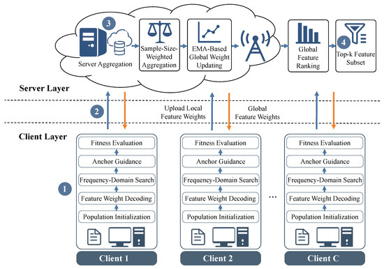
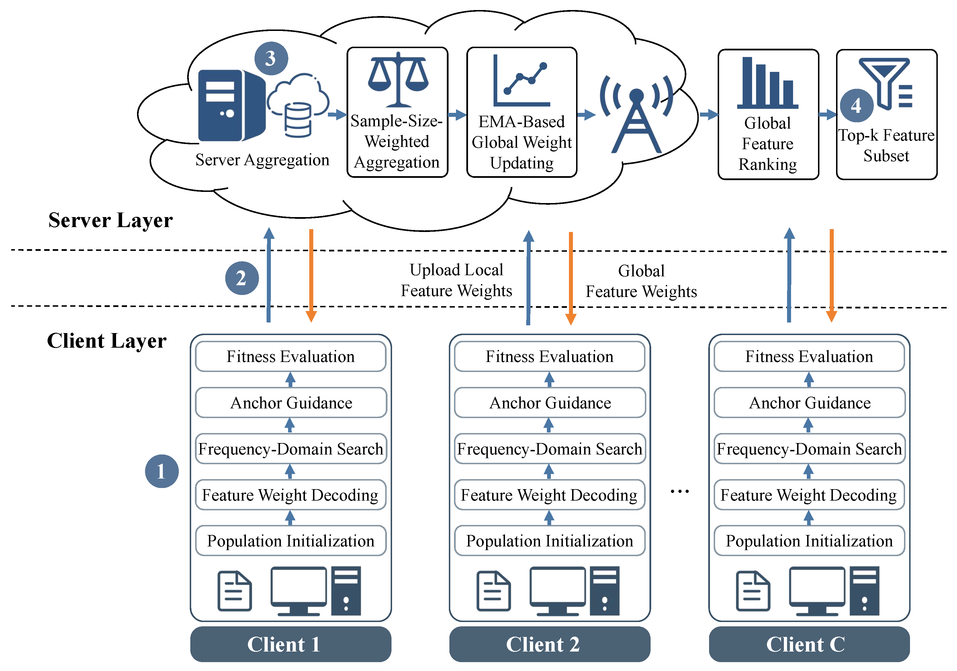
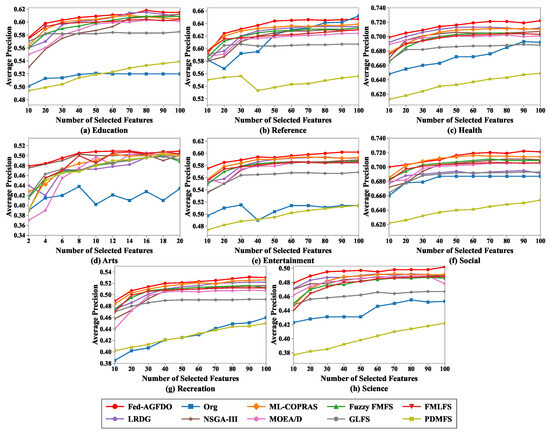
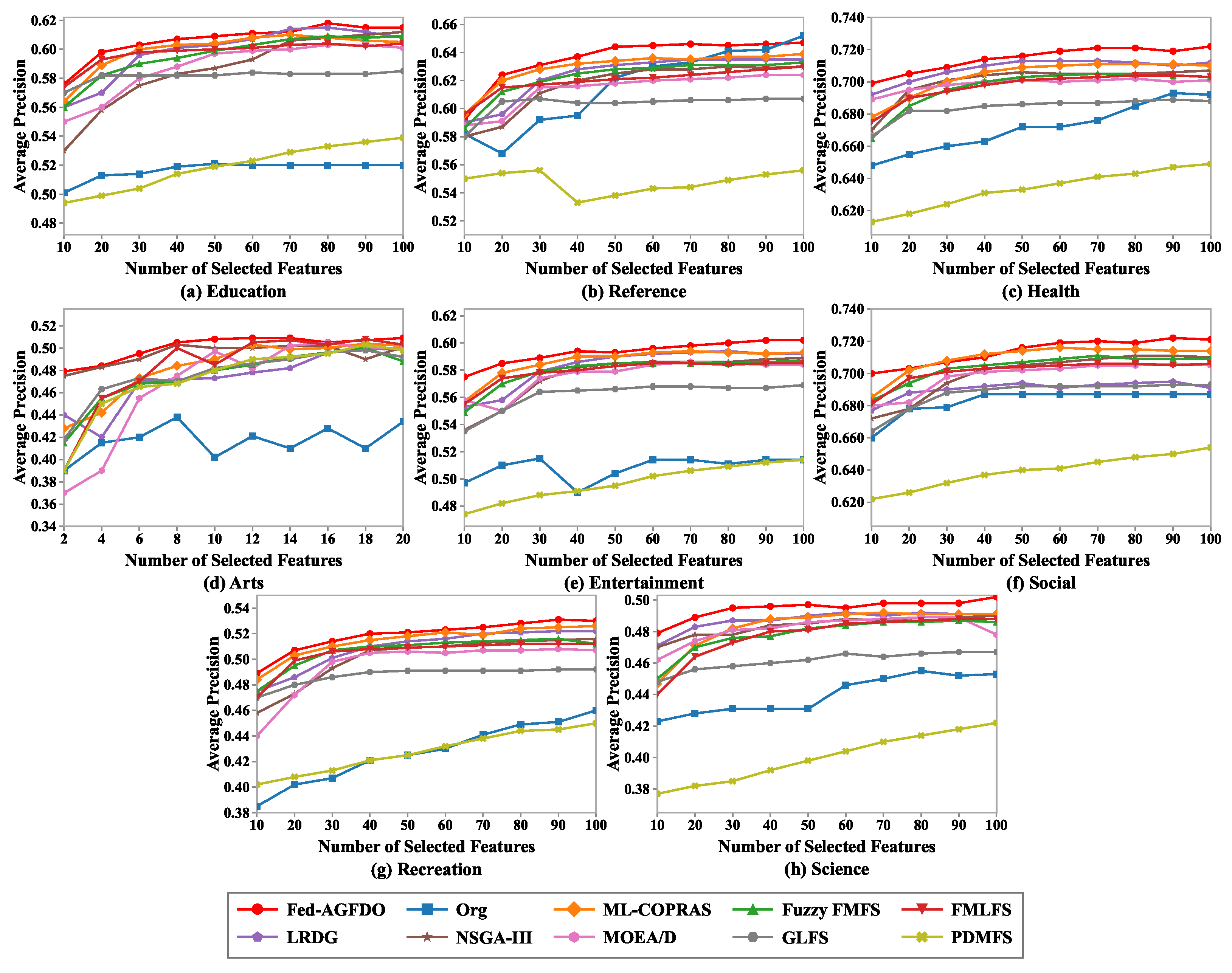
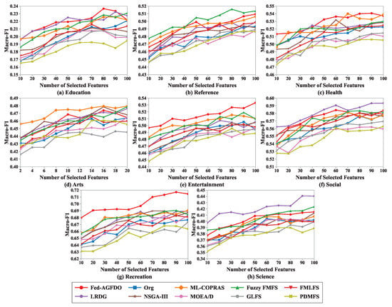
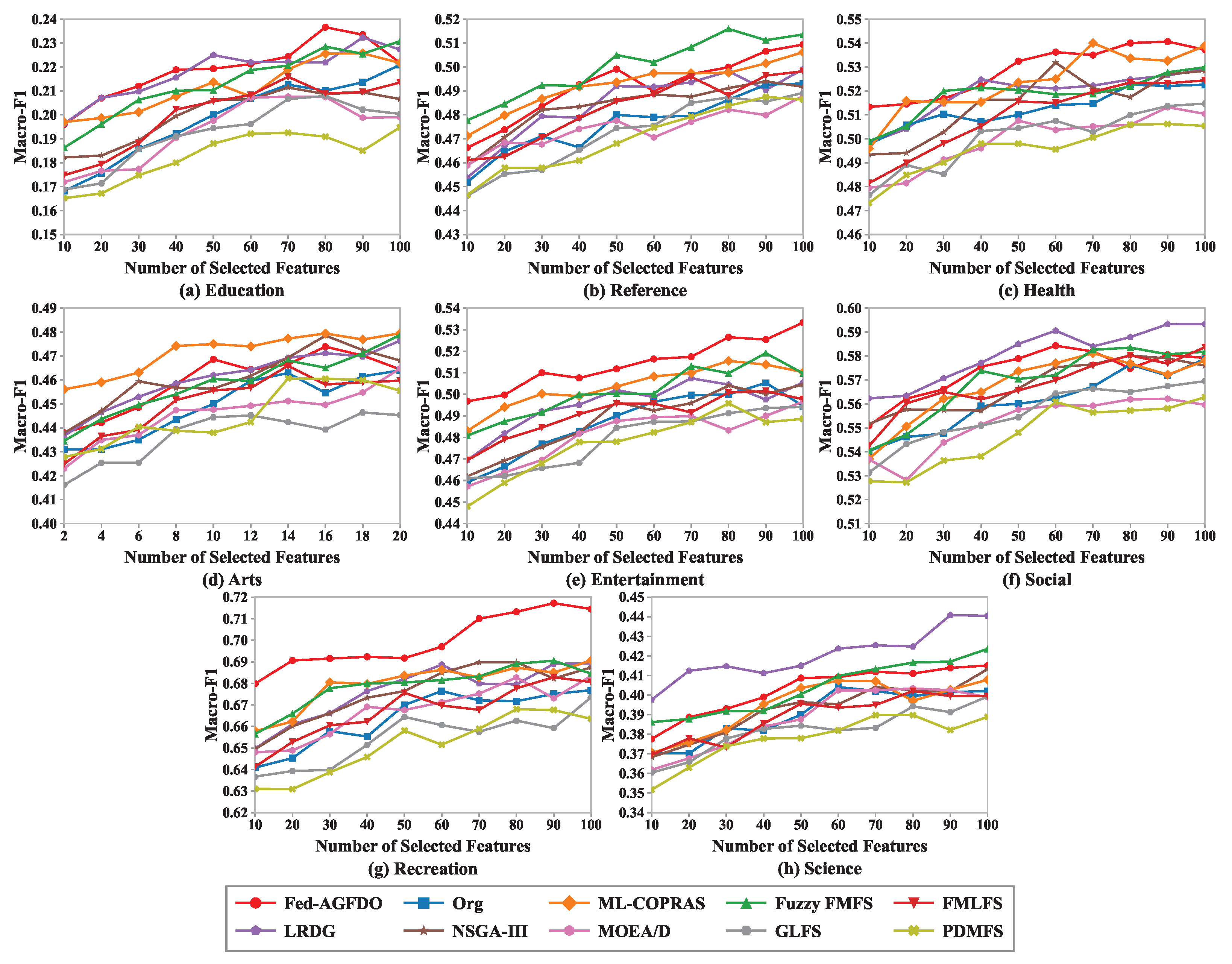
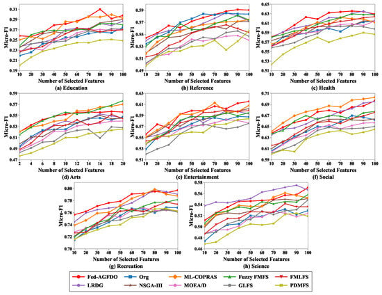
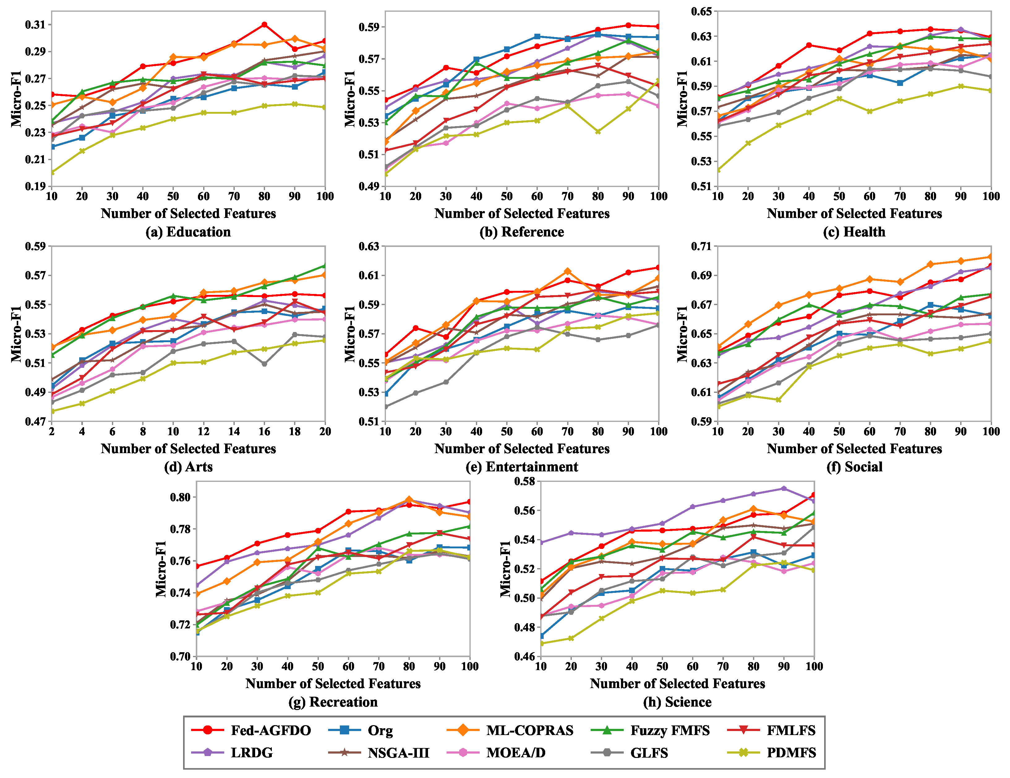
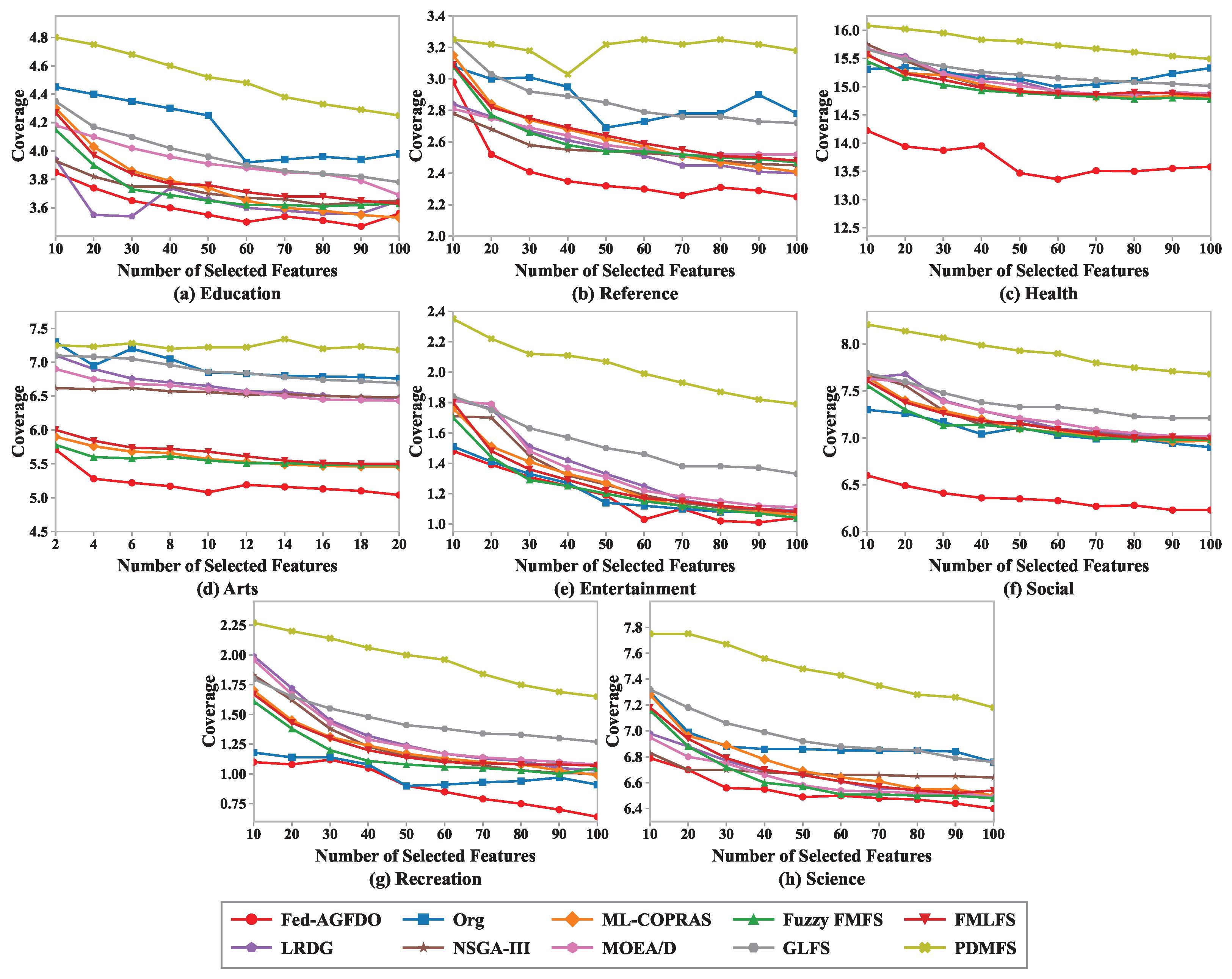
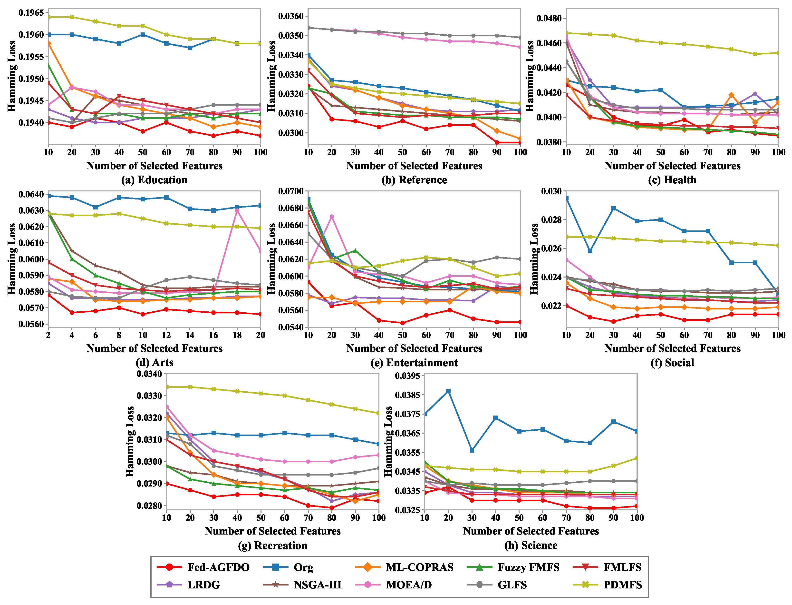
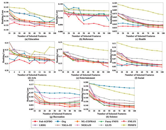
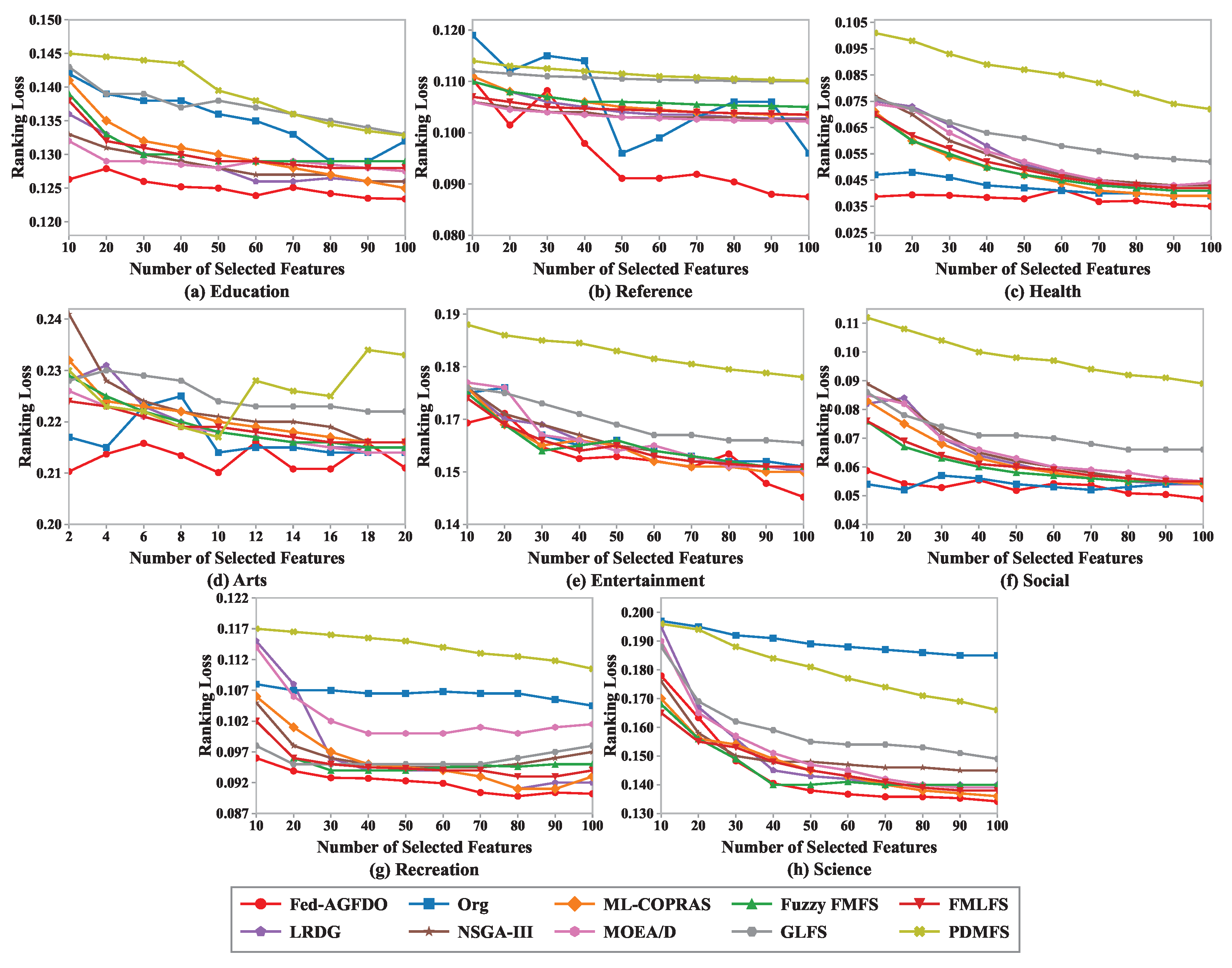
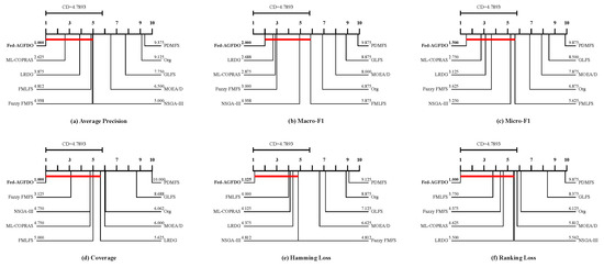
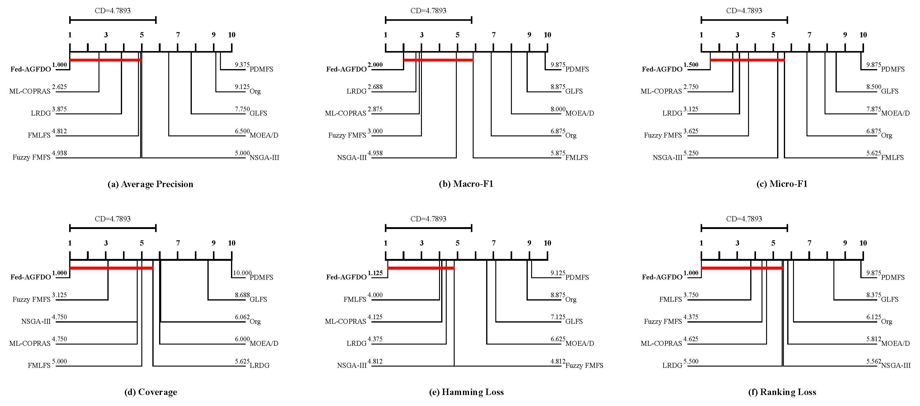
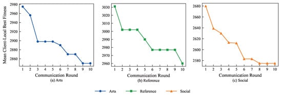

Disclaimer/Publisher’s Note: The statements, opinions and data contained in all publications are solely those of the individual author(s) and contributor(s) and not of MDPI and/or the editor(s). MDPI and/or the editor(s) disclaim responsibility for any injury to people or property resulting from any ideas, methods, instructions or products referred to in the content. |
© 2026 by the authors. Licensee MDPI, Basel, Switzerland. This article is an open access article distributed under the terms and conditions of the Creative Commons Attribution (CC BY) license.