Computing Well-Balanced Spanning Trees of Unweighted Networks

Abstract

A spanning tree of a network or graph is a subgraph that connects all nodes with the minimum number or total weight of edges. Spanning trees are among the simplest yet most effective techniques for network simplification, sampling, and uncovering a network’s backbone or skeleton. Prim’s algorithm and Kruskal’s algorithm are well-known algorithms for computing a spanning tree of a weighted network, and are therefore also the default procedure for unweighted networks in the most popular network libraries. In this paper, we empirically evaluate the performance of these algorithms on unweighted networks and compare them with priority-first search algorithms. We show that the distances between the nodes are better preserved by a simpler algorithm based on breadth-first search. The spanning trees are also more compact and well-balanced, as measured by classical graph indices. We support our findings with experiments on synthetic graphs and over a thousand real networks, and demonstrate the practical applications of the computed spanning trees. We conclude that for preserving the structure of an unweighted network, the breadth-first search algorithm should be the preferred choice.

1. Introduction

Networks or graphs have become a popular tool for analyzing complex real-world systems [1]. Examples include predicting the spread of contagious viruses [2], the study of the interactome of species [3], understanding the structure of science [4] and outreach of online social connections [5]. The size of today’s networks is often in millions of nodes and edges, with the largest networks being the WWW with more than a trillion web pages and the human brain with nearly a hundred billion neurons. As a result, the size of real networks makes many practical applications computationally very challenging.

Techniques to alleviate this issue include network simplification or sampling [6,7,8] and revealing the so-called network backbone or skeleton [9,10,11,12]. These approaches try to reduce the size of a network in a way that the network still retains many of its structural properties. One of the most straightforward ways to simplify a network is to compute its spanning tree [1,13], which is a subgraph connecting all the nodes of a network with the minimum number of edges. Spanning trees retain the connectivity of networks and possibly other structural properties, and have gained considerable interest in recent years [14,15,16,17,18]. In the case of weighted networks, one usually aims to compute the minimum spanning tree, which is a subgraph connecting all the nodes with the minimum total weight of the edges. In the case of unweighted networks, any spanning tree is, in fact, a “minimum” spanning tree.

Prim’s and Kruskal’s algorithms are well-known algorithms for computing a minimum spanning tree of a weighted network [1,13]. Although the algorithms were primarily developed for weighted networks, they can be readily applied to unweighted networks where each edge has the same weight. This is also the default procedure in the most popular network analysis libraries NetworkX, igraph, and graph-tool [19]. However, the performance of these algorithms has not been sufficiently studied for unweighted networks, which are much more common in practical applications [20]. In particular, there exist no theoretical guarantees for the algorithms, and neither does the literature provide any empirical comparison on large-scale networks.

Problem Statement

A fundamental result of metric embedding theory, Bourgain’s theorem [21], states that any finite metric space can be embedded into a tree metric with logarithmic distortion. This suggests that while spanning trees provide a reasonable approximation of network structure, they inevitably introduce some bias that must be evaluated empirically.

In this paper, we compare different algorithms for computing spanning trees of unweighted networks. While standard network properties, such as connectivity, average degree, and clustering coefficients [22,23], are fixed by the construction of a spanning tree, we focus on the distances between nodes in a network, as well as the balance and compactness of the resulting spanning trees as measured by Wiener’s index [24] and Sackin’s index [25]. Since distances in a spanning tree can only increase relative to the original network, we empirically evaluate which algorithms minimize the average and maximum distances, both globally and at the level of individual nodes. These structural properties are crucial for a wide range of practical applications.

We do not frame our problem as an optimization task. Instead, we compare existing efficient algorithms, readily available in network analysis libraries, with priority-first search approaches across various synthetic graphs and over a thousand real networks. In particular, we demonstrate that, for unweighted networks, a spanning tree computed using breadth-first search best preserves the network’s structural properties.

2. Methods and Data

2.1. Definitions and Notations

Let a network be represented by an undirected connected graph $G=(V,E)$, where V denotes the set of nodes of G and E denotes the set of edges of G. Where necessary to make explicit that these sets represent the graph G, we write $V_G$ and $E_G$. The number of nodes equals $n=\left|V\right|$ and the number of edges equals $m=\left|E\right|$. We denote the average node degree as $⟨k⟩=2m/n$. Furthermore, let $d_{ij}$ be the distance between the nodes $i,j\in V$, defined as the number of edges in a shortest path between the nodes i and j. Since the graph is undirected and connected, $d_{ij}=d_{ji}$ and $d_{ij}<\infty$. Therefore, the average distance between the nodes equals $⟨d⟩={\displaystyle \frac{2}{n(n-1)}}{\sum }_{i<j}{d}_{ij}$ and the maximum distance or diameter equals $d_{\max }={max}_{i<j}{d}_{ij}$. In order to measure the variability of the distances between the nodes, we also define the coefficient of variation as $c_d={\sigma }_d/⟨d⟩$, where ${\sigma }_d$ is the standard deviation of distances. The coefficient of variation $c_d$ is a measure of the dispersion of a probability distribution, where the distributions with $c_d<1$ are considered low-variance distributions, while those with $c_d>1$ are considered high-variance distributions.

2.2. Spanning Tree Algorithms

Below, we briefly describe the algorithms for computing a spanning tree of an undirected connected graph. In the case of a disconnected graph consisting of more than one connected component, the algorithms should be applied to each connected component separately. The implementation of these algorithms is included in most standard network analysis libraries, while their pseudocode and a discussion of complexity are provided in Appendix A.

Note that any algorithm below can, in principle, compute any spanning tree of a given graph. The specific tree depends on the random choices made within the algorithm or, equivalently, on the ordering of nodes and edges in the memory. However, as we demonstrate in this paper, the structural properties of the spanning trees computed by different algorithms do, in fact, differ.

2.2.1. Prim’s Algorithm

Prim’s algorithm for computing a spanning tree operates as follows. First, the algorithm selects a random seed node and adds it to an empty tree. Then, on each step of the algorithm, a random edge from the graph is selected that leads from a node already in the tree to a node not yet in the tree. Finally, when there is no further node in the graph that is not already in the tree, the algorithm stops. At this point, the resulting tree is a spanning tree of the graph.

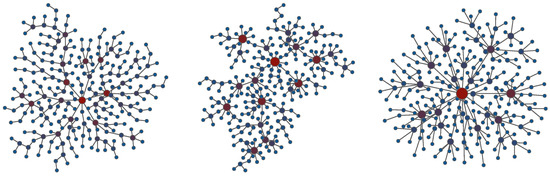
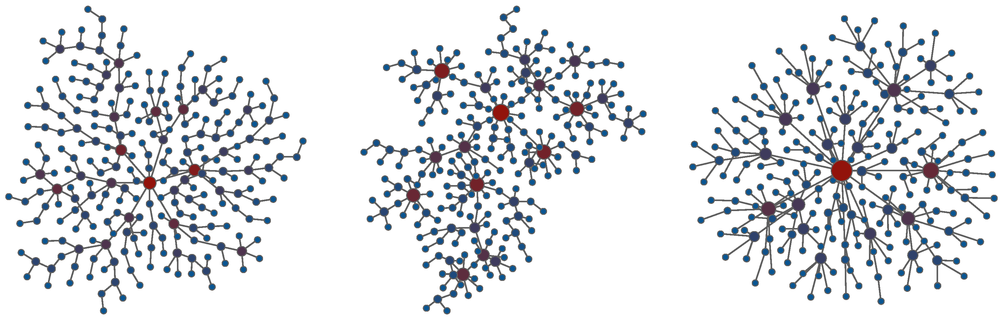
Prim’s algorithm is nondeterministic, whereas the actual spanning tree depends on a random selection of the seed node and the edges to expand the tree. As a representative example, the left graph in Figure 1 shows a spanning tree computed with Prim’s algorithm.

Figure 1. Wiring diagrams of spanning trees of a small random graph. The spanning trees were computed with Prim’s algorithm (left), Kruskal’s algorithm (middle) and the breadth-first search algorithm (right). The size of the nodes is proportional to their degree, while the layouts were computed with the Large Graph Layout algorithm [26].

2.2.2. Kruskal’s Algorithm

Kruskal’s algorithm differs conceptually from Prim’s algorithm. Instead of starting with a tree consisting of a seed node and then expanding it, the algorithm begins with a forest of trees, each consisting of a single node. The trees are then incrementally merged into larger trees by adding edges between them until only one remains. At this point the algorithm stops and the resulting tree is a spanning tree of a graph.

Kruskal’s algorithm is nondeterministic, whereas the actual spanning tree depends on a random selection of the edges to merge the trees. As a representative example, the middle graph in Figure 1 shows a spanning tree computed with Kruskal’s algorithm.

2.2.3. Breadth-First Search

The breadth-first search node traversal is very similar to Prim’s algorithm. The main difference is in how the edges to non-visited nodes are processed. In contrast to Prim’s algorithm, which processes only one such edge at each step, the breadth-first search processes all edges from a selected node to non-visited nodes in a single step.

The breadth-first search algorithm is also a standard approach for computing the distances between one selected node and all other nodes in an undirected network. The algorithm is again nondeterministic, whereas the actual spanning tree depends on a random selection of the seed node and the order in which the edges are processed. As a representative example, the right graph in Figure 1 shows a spanning tree computed with the breadth-first search algorithm.

2.2.4. Other Algorithms

Other algorithms for computing a spanning tree include Sollin’s algorithm, which can be seen as a combination of Prim’s and Kruskal’s approaches. Another popular algorithm for computing a spanning tree of a weighted graph using parallel processing is Borůvka’s algorithm. However, in the case of non-distinct edge weights, as is the case in unweighted graphs, a consistent tie-breaking mechanism must be applied by adopting some fixed total ordering of the nodes or edges.

Note that a spanning tree of an unweighted graph can be computed by any graph traversal algorithm, provided that the algorithm ensures that no cycles are created during the construction of the tree. Besides breadth-first search, this includes depth-first search, beam search, fores fire, and other traversal algorithms. While the breadth-first search algorithm processes nodes in a graph using a level-order traversal, the depth-first search algorithm uses a preorder traversal. On the other hand, the beam search algorithm can be seen as a heuristic compromise between breadth-first search and Prim’s algorithm.

2.3. Tree Balance Index

In the language of computational theory, a balanced tree is a data structure where the time complexity of standard operations such as adding or deleting an element is $\mathcal{O}\left(\log n\right)$ for any practical definition of balance [27]. Consider a rooted tree T with root $r\in V_T$ and let ${\tilde{V}}_T\subseteq V_T\setminus \left\{r\right\}$ be the set of tree leaves (i.e., degree-1 nodes). Then, balance implies that the distance $d_{ir}$ between all leaf nodes $i\in {\tilde{V}}_T$ and the root $r\in V_T$ is at most $\mathcal{O}\left(\log n\right)$, which further implies that the average distance between all pairs of nodes $⟨d⟩$ and also the diameter $d_{\max }$ are in $\mathcal{O}\left(\log n\right)$, since one can always take a path through the root. However, in the case of a random tree, both values are almost certainly in $\mathcal{O}\left(\sqrt{n}\right)$ [28,29].

Phylogenetics literature defines various indices of tree balance [30,31] that quantify the branching symmetry and compactness of trees. One of the most widely used is Sackin’s index of imbalance [25]. Sackin’s index is defined as the sum of the number of nodes between all leaves $i\in {\tilde{V}}_T$ and the root $r\in V_T$, which is included in the count. This can be equivalently written as ${\sum }_{i\in {\tilde{V}}_T}{d}_{ir}$. Since Sackin’s index tends to increase with the number of nodes, we normalize by the minimum possible value $\tilde{n}=\left|{\tilde{V}}_T\right|$, which is reached on the star tree, and the maximum possible value $(\tilde{n}+2)(\tilde{n}-1)/2$, which is reached on the caterpillar tree. The normalized Sackin’s index S [32] is then defined as

$$\begin{array}{c}\hfill S={\displaystyle \frac{{\sum }_{i\in {\tilde{V}}_T}{d}_{ir}-\tilde{n}}{(\tilde{n}+2)(\tilde{n}-1)/2-\tilde{n}}},\end{array}$$

(1)

where smaller values correspond to more balanced trees.

For spanning trees computed with the breadth-first search and Prim’s algorithms, we designate the randomly selected seed node as the root. Spanning trees computed with Kruskal’s algorithm, on the other hand, do not have a naturally defined root. We, therefore, randomly select different nodes as the root and average the results.

2.4. Collections of Networks

Table 1 shows statistics of collections of more than a thousand real networks analyzed in the paper. These represent citations between the papers published in the journal Physical Review E [33], paper collaborations between Slovenian researchers extracted from the SICRIS database [34], protein interactions of different species collected from the BioGRID repository [35,36], interactions between the users at the stack exchange web site MathOverflow [37,38], Facebook friendships between the students at different US universities [39,40] and links between autonomous systems extracted by the Oregon Route Views project [38,41]. Some collections represent temporal networks that grow through time (e.g., paper citations and author collaborations), while other represent similar networks of different size (e.g., protein interactions and online friendships). All networks were reduced to a simple graph of their largest connected component.

Table 1. Statistics of collections of real networks.

Collection	Networks N	Nodes n	Edges m	Degree $⟨\mathit{k}⟩$	Distance $⟨\mathit{d}⟩$	Clustering $⟨\mathit{C}⟩$
Paper citations	46	$[3,37,511]$	$[2,135,260]$	$[1.3,7.2]$	$[1.33,21.79]$	$[0.00,0.27]$
Author collaborations	25	$[18,1735]$	$[42,6710]$	$[4.1,7.7]$	$[1.85,8.75]$	$[0.46,0.75]$
Protein interactions	40	$[5,19,961]$	$[4,238,886]$	$[1.6,83.1]$	$[1.47,6.06]$	$[0.00,0.52]$
User interactions	75	$[2,20,969]$	$[1,86,137]$	$[1.0,10.1]$	$[1.00,3.80]$	$[0.00,0.17]$
Online friendships	97	$[762,41,536]$	$[16,651,1,590,651]$	$[39.1,116.2]$	$[2.24,3.21]$	$[0.19,0.41]$
Autonomous systems	733	$[103,6474]$	$[239,12,572]$	$[3.4,4.7]$	$[2.65,3.98]$	$[0.16,0.29]$

The statistics include the number of networks in the collection N, the number of nodes n and edges m, the average node degree $⟨k⟩$, the average distance between the nodes $⟨d⟩$ and the average node clustering coefficient $⟨C⟩$.

3. Results

3.1. Motivating Example

As a motivating example, we consider an Erdős–Rényi random graph [42] with n nodes and the probability of an edge between each pair of nodes $p=⟨k⟩/(n-1)$, where $⟨k⟩$ is the expected node degree. We focus on the average distance between nodes $⟨d⟩$ and the diameter $d_{\max }$. A theoretical estimate for the diameter $d_{\max }$ of a random graph equals $\log n/\log ⟨k⟩$ [1], which is $d_{\max }=2.40$ for $n=250$ and $⟨k⟩=10$. Due to the sensitivity of the diameter $d_{\max }$ for small n and $⟨k⟩$, this is a better estimate of the average distance between the nodes $⟨d⟩$. Indeed, the empirical estimates with standard deviations over a thousand realizations of the considered random graphs are $⟨d⟩\approx 2.66\pm 0.01$ and $d_{\max }\approx 4.46\pm 0.50$.

Figure 1 shows particular realizations of spanning trees of such random graphs computed using Prim’s algorithm, Kruskal’s algorithm and the breadth-first search algorithm. The empirical estimates of diameter $d_{\max }$ of the spanning trees equal $19.18\pm 1.89$, $20.06\pm 2.58$ and $7.58\pm 0.57$, respectively. While the diameters of the spanning trees computed with Prim’s and Kruskal’s algorithms are much higher than in the random graphs, the diameter of the spanning tree computed with the breadth-first search algorithm is much closer.

Despite the structural differences observed between the spanning trees computed by different algorithms, any algorithm can, in principle, compute any spanning tree of a graph. When comparing spanning trees using the graph edit distance, which is defined as the number of edge insertions or deletions required to transform one tree into another, the trees produced by a single algorithm are not much more similar to each other than those produced by different algorithms. For the random graphs considered above, the edit distances between the spanning trees computed by Prim’s algorithm and by the breadth-first search algorithm are $389.9\pm 11.7$ and $391.6\pm 26.9$, respectively, whereas the edit distance between trees produced by the two algorithms is $395.7\pm 12.4$.

3.2. Synthetic Graphs

In this section, we study the scaling of the average distance $⟨d⟩$ and the diameter $d_{\max }$ of spanning trees of graphs with an increasing number of nodes n and empirically estimate whether the values scale as $\mathcal{O}\left(\log n\right)$ or worse. Note that only in the case of the former, the spanning trees can possibly retain short distances between the nodes in real small-world networks [22].

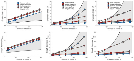
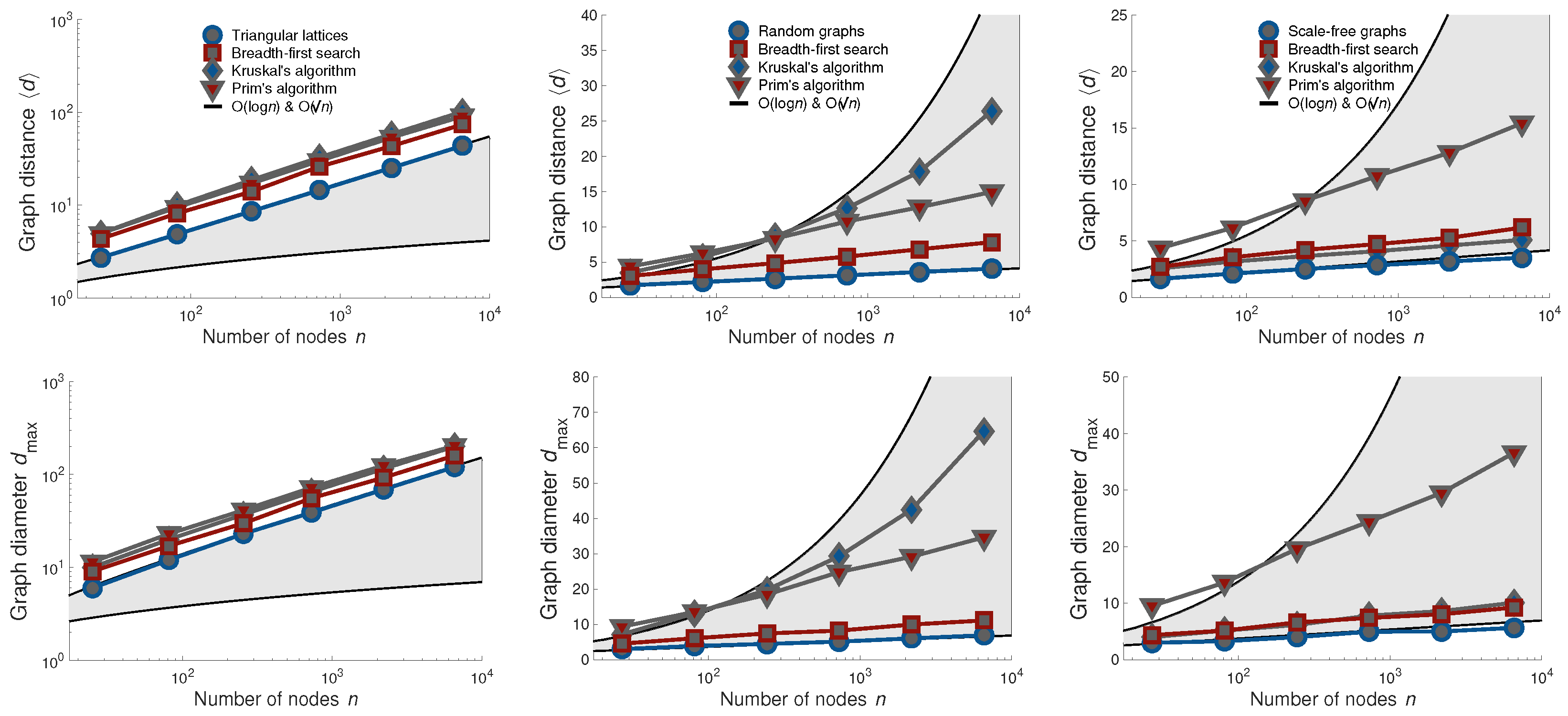
We analyse triangular lattices, Erdős–Rényi random graphs [42] and Barabási–Albert scale-free graphs [43]. We vary the number of nodes n, while we keep the average node degree of random and scale-free graphs fixed to $⟨k⟩=10$. Figure 2 shows the scaling of the average distance $⟨d⟩$ and the diameter $d_{\max }$ for synthetic graphs and their spanning trees computed with different algorithms.

Figure 2. The average distance $⟨d⟩$ and the diameter $d_{\max }$ of triangular lattices (left), random graphs (middle) and scale-free graphs (right), and their spanning trees computed with different algorithms. The plots show estimates over 100 realizations, where the shaded areas span between theoretical estimates for random graphs $\mathcal{O}\left(\log n\right)$ and two-dimensional lattices $\mathcal{O}\left(\sqrt{n}\right)$, and are consistent between the plots.

We first consider triangular lattices, as these results serve as a baseline for further analyses. The average distance $⟨d⟩$ and the diameter $d_{\max }$ of any two-dimensional lattice scale as $\mathcal{O}\left(\sqrt{n}\right)$ [1]. This can be observed as a straight line with slope $0.5$ on double logarithmic plots in the left column of Figure 2. Notice that all spanning trees computed with different algorithms show similar scaling $\mathcal{O}\left(\sqrt{n}\right)$.

Next, we consider Erdős–Rényi random graphs [42] shown in the middle column of Figure 2. The average distance $⟨d⟩$ and the diameter $d_{\max }$ of random graphs, and also small-world networks [22], scale as $\mathcal{O}\left(\log n\right)$ [1]. This can be observed as a straight line on semi-logarithmic plots in Figure 2, whereas any upward concave function would imply a faster scaling than $\mathcal{O}\left(\log n\right)$. Notice that the spanning trees computed with the breadth-first search algorithm best preserve the distances in random graphs, while both the average distance $⟨d⟩$ and the diameter $d_{\max }$ appear to scale as $\mathcal{O}\left(\log n\right)$, at least for a moderate number of nodes $n\le {10}^4$. In contrast, the distances between the nodes of the spanning trees computed with Kruskal’s algorithm scale faster than $\mathcal{O}\left(\log n\right)$ (see also Figure 3 and the discussion alongside).

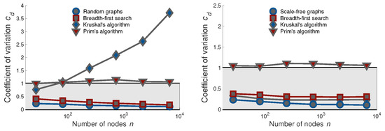
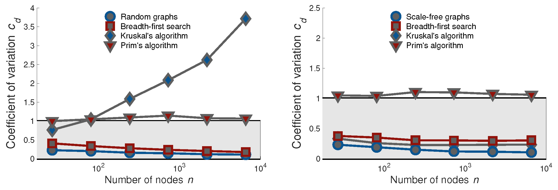
Figure 3. The coefficient of variation $c_d$ for random graphs (left) and scale-free graphs (right), and their spanning trees computed with different algorithms. The plots show estimates over 100 realizations, while the error bars are smaller than the symbol sizes.

Last, we consider Barabási–Albert scale-free graphs [43] shown in the right column of Figure 2. The average distance $⟨d⟩$ and the diameter $d_{\max }$ of scale-free graphs scale as $\mathcal{O}(\log n/\log \log n)$ [44], while such graphs are usually called ultra small-world [45]. Note that $\mathcal{O}(\log n/\log \log n)$ is indistinguishable from $\mathcal{O}\left(\log n\right)$ for $n\le {10}^4$, thus this scaling can again be observed as a straight line on semi-logarithmic plots in Figure 2. The spanning trees computed with both the breadth-first search algorithm and Kruskal’s algorithm well retain the distances between the nodes of scale-free graphs and appear to scale as $\mathcal{O}\left(\log n\right)$. On the other hand, the distances between the nodes of the spanning trees computed with Prim’s algorithm can be more than five times larger than the distances in scale-free graphs (e.g., $⟨d⟩=15.42$ and $d_{\max }=36.60$ compared to $3.51$ and $5.64$ for graphs with $n=6561$ nodes).

The above observations are confirmed in Figure 3, where we show the coefficient of variation of the distances between the nodes $c_d$. Note that the distributions of the distances between the nodes in random and scale-free graphs, and real small-world networks, are low-variance with $c_d\ll 1$ [22,45]. As one can observe in Figure 3, all distributions of the distances in the spanning trees computed with the breadth-first search algorithm are low-variance $c_d\ll 1$. On the other hand, the distributions in the spanning trees computed with Kruskal’s algorithm are high-variance $c_d\gg 1$ for random graphs with $n>100$, while the results for Prim’s algorithm are inconclusive $c_d\approx 1$.

To summarize, only spanning trees computed with the breadth-first search algorithm retain short distances between the nodes of random and scale-free graphs. In the next section, we consider real networks.

3.3. Real Networks

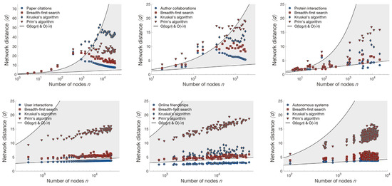
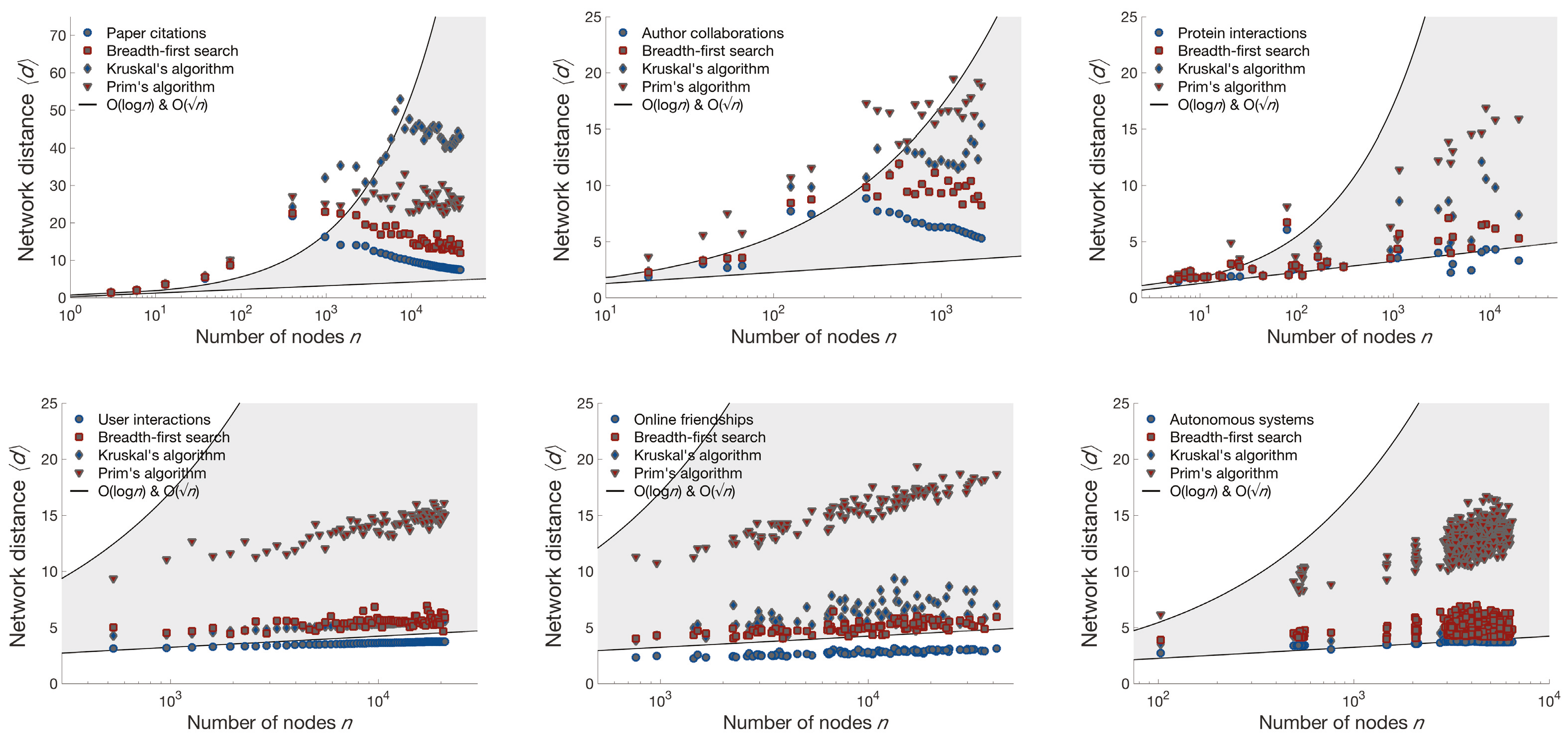
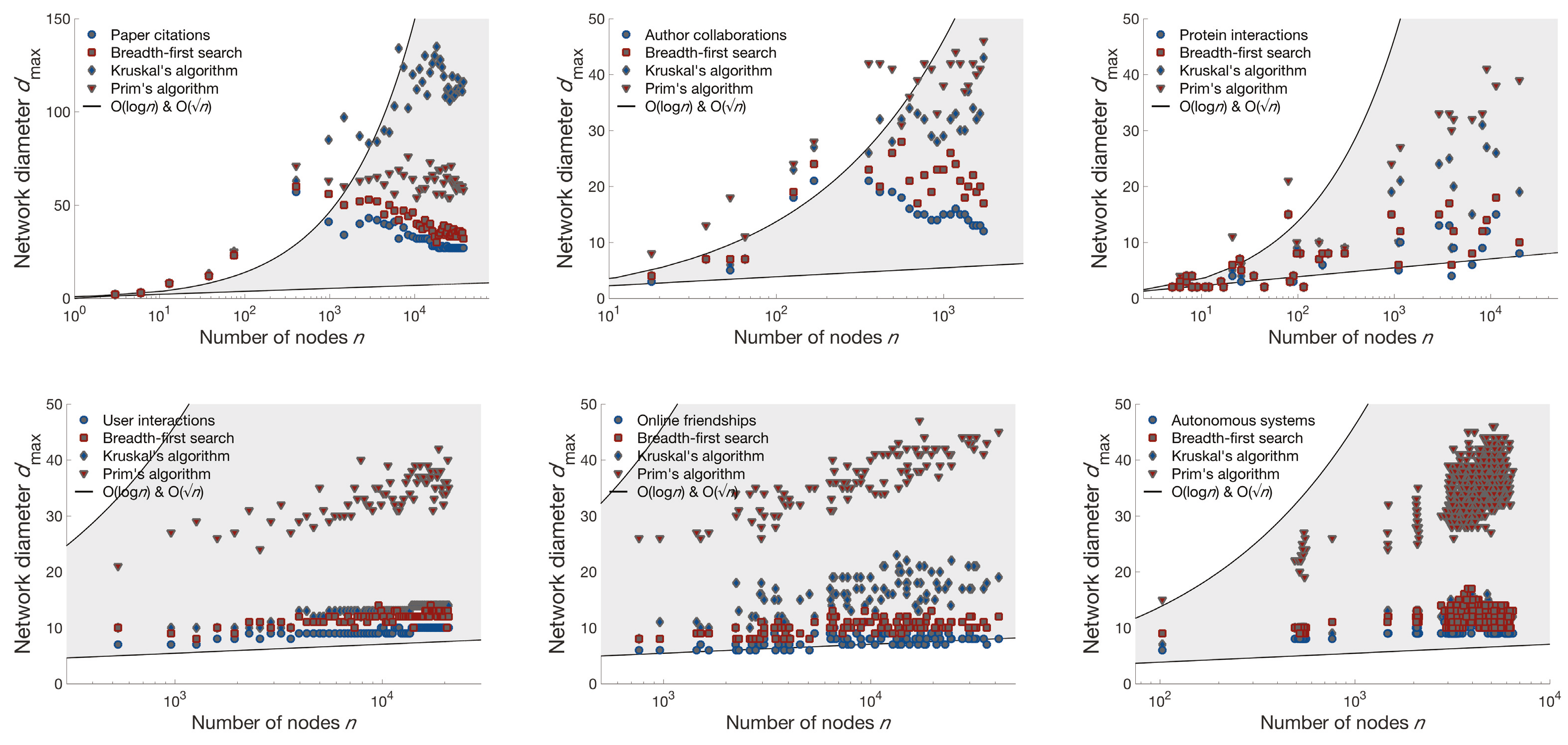
Figure 4 shows the average distance between the nodes $⟨d⟩$ in real networks and their spanning trees, where we have used semi-logarithmic axes as in Figure 2. First, we consider the networks. As expected for small-world networks [22], the average distance $⟨d⟩$ increases with the number of nodes n and appears to scale no faster than $\mathcal{O}\left(\log n\right)$ in all network collections but two. In the case of temporal networks representing paper citations and author collaborations in the first two plots of Figure 4, the average distance $⟨d⟩$ actually starts to decrease when the number of nodes exceeds $n\approx 500$. This is a consequence of network densification known as a shrinking diameter [41]. Figure 5 shows also the diameter $d_{\max }$ of real networks, where the interpretation is exactly the same.

Figure 4. The average distance $⟨d⟩$ in real networks and their spanning trees computed with different algorithms. The shaded areas are the same as in Figure 2.

Figure 5. The diameter $d_{\max }$ of real networks and their spanning trees computed with different algorithms. The shaded areas are the same as in Figure 2.

Next, we consider the spanning trees of these networks computed with different algorithms. Consistent with the results for synthetic graphs, the spanning trees computed with the breadth-first search algorithm best preserve the average distance between the nodes $⟨d⟩$ in all network collections but two. In the case of networks representing user interactions and autonomous systems in the bottom row of Figure 4, Kruskal’s algorithm performs similarly, although the differences in the average distance $⟨d⟩$ are very small. Furthermore, in non-temporal networks that are not subject to the densification law [41], the average distance $⟨d⟩$ of the spanning trees computed with the breadth-first search algorithm appears to scale no faster than $\mathcal{O}\left(\log n\right)$, while in other networks, the scaling of the average distance $⟨d⟩$ closely follows the scaling in real networks. Again, Figure 5 shows also the diameter $d_{\max }$ of spanning trees, where the interpretation is the same.

Table 2 shows the percentage of networks for which the average distance $⟨d⟩$ of spanning trees computed with the breadth-first search algorithm differs from that of Prim’s algorithm and Kruskal’s algorithm. As noted above, the average distance $⟨d⟩$ of spanning trees computed with Kruskal’s algorithm is lower in more than half of the networks representing user interactions and autonomous systems. However, the differences are only minor. Furthermore, Table 3 shows the same results for the diameter $d_{\max }$ of spanning trees, where the breadth-first search algorithm consistently outperforms the other two algorithms.

Table 2. The percentage of real networks for which the average distance $⟨d⟩$ of spanning trees differs.

	Breadth-First Search vs. Prim’s alg.			Breadth-First Search vs. Kruskal’s alg.
Collection	${⟨\mathit{d}⟩}^{\mathrm{B}}<{⟨\mathit{d}⟩}^{\mathrm{P}}$	${⟨\mathit{d}⟩}^{\mathrm{B}}={⟨\mathit{d}⟩}^{\mathrm{P}}$	${⟨\mathit{d}⟩}^{\mathrm{B}}>{⟨\mathit{d}⟩}^{\mathrm{P}}$	${⟨\mathit{d}⟩}^{\mathrm{B}}<{⟨\mathit{d}⟩}^{\mathrm{K}}$	${⟨\mathit{d}⟩}^{\mathrm{B}}={⟨\mathit{d}⟩}^{\mathrm{K}}$	${⟨\mathit{d}⟩}^{\mathrm{B}}>{⟨\mathit{d}⟩}^{\mathrm{K}}$
Paper citations	$95.7\%$	$4.3\%$	$0.0\%$	$95.7\%$	$4.3\%$	$0.0\%$
Author collaborations	$100.0\%$	$0.0\%$	$0.0\%$	$84.0\%$	$4.0\%$	$12.0\%$
Protein interactions	$57.5\%$	$42.5\%$	$0.0\%$	$42.5\%$	$47.5\%$	$10.0\%$
User interactions	$98.7\%$	$1.3\%$	$0.0\%$	$32.0\%$	$1.3\%$	$66.7\%$
Online friendships	$100.0\%$	$0.0\%$	$0.0\%$	$87.6\%$	$0.0\%$	$12.4\%$
Autonomous systems	$100.0\%$	$0.0\%$	$0.0\%$	$46.9\%$	$0.0\%$	$53.1\%$

For a graphical representation of the average distance $⟨d⟩$ of spanning trees, see Figure 4.

Table 3. The percentage of real networks for which the diameter $d_{\max }$ of spanning trees differs.

	Breadth-First Search vs. Prim’s alg.			Breadth-First Search vs. Kruskal’s alg.
Collection	${\mathit{d}}_{\max }^{\mathrm{B}}<{\mathit{d}}_{\max }^{\mathrm{P}}$	${\mathit{d}}_{\max }^{\mathrm{B}}={\mathit{d}}_{\max }^{\mathrm{P}}$	${\mathit{d}}_{\max }^{\mathrm{B}}>{\mathit{d}}_{\max }^{\mathrm{P}}$	${\mathit{d}}_{\max }^{\mathrm{B}}<{\mathit{d}}_{\max }^{\mathrm{K}}$	${\mathit{d}}_{\max }^{\mathrm{B}}={\mathit{d}}_{\max }^{\mathrm{K}}$	${\mathit{d}}_{\max }^{\mathrm{B}}>{\mathit{d}}_{\max }^{\mathrm{K}}$
Paper citations	$91.3\%$	$8.7\%$	$0.0\%$	$93.5\%$	$6.5\%$	$0.0\%$
Author collaborations	$100.0\%$	$0.0\%$	$0.0\%$	$84.0\%$	$12.0\%$	$4.0\%$
Protein interactions	$50.0\%$	$50.0\%$	$0.0\%$	$37.5\%$	$55.0\%$	$7.5\%$
User interactions	$98.7\%$	$1.3\%$	$0.0\%$	$82.7\%$	$12.0\%$	$5.3\%$
Online friendships	$100.0\%$	$0.0\%$	$0.0\%$	$95.9\%$	$4.1\%$	$0.0\%$
Autonomous systems	$100.0\%$	$0.0\%$	$0.0\%$	$62.3\%$	$20.6\%$	$17.1\%$

For a graphical representation of the diameter $d_{\max }$ of spanning trees, see Figure 5.

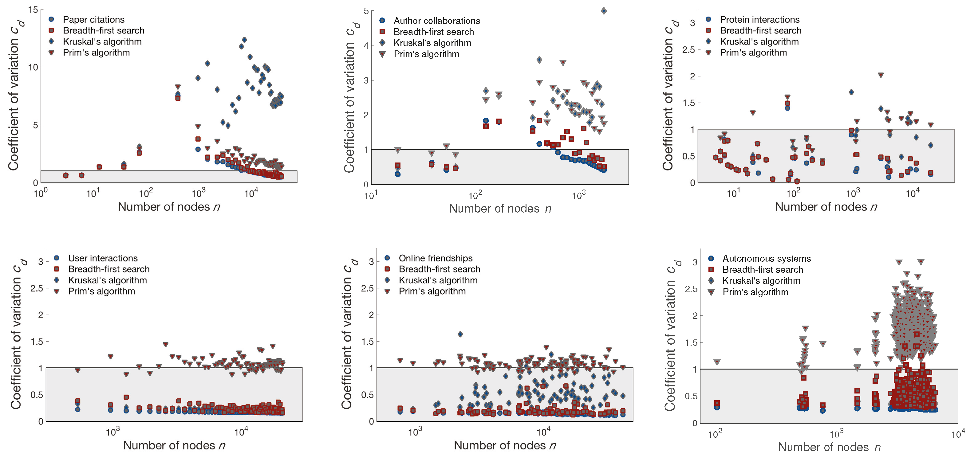
The above observations are confirmed in Figure 6 and Table 4, where we show the coefficient of variation of the distances between the nodes $c_d$. Notice that all distributions of the distances in real networks and spanning trees computed with the breadth-first search algorithm are low-variance with $c_d<1$, as long as the networks are large enough $n\ge {10}^4$. In contrast, this holds neither for Kruskal’s algorithm nor Prim’s algorithm, where even $c_d\gg 1$ for some network collections (see first and last plot of Figure 6).

Figure 6. The coefficient of variation $c_d$ for real networks and their spanning trees computed with different algorithms. Other details are the same as in Figure 3.

Table 4. The percentage of real networks for which the coefficient of variation $c_d$ of spanning trees differs.

	Breadth-First Search vs. Prim’s alg.			Breadth-First Search vs. Kruskal’s alg.
Collection	${\mathit{c}}_{\mathit{d}}^{\mathrm{B}}<{\mathit{c}}_{\mathit{d}}^{\mathrm{P}}$	${\mathit{c}}_{\mathit{d}}^{\mathrm{B}}={\mathit{c}}_{\mathit{d}}^{\mathrm{P}}$	${\mathit{c}}_{\mathit{d}}^{\mathrm{B}}>{\mathit{c}}_{\mathit{d}}^{\mathrm{P}}$	${\mathit{c}}_{\mathit{d}}^{\mathrm{B}}<{\mathit{c}}_{\mathit{d}}^{\mathrm{K}}$	${\mathit{c}}_{\mathit{d}}^{\mathrm{B}}={\mathit{c}}_{\mathit{d}}^{\mathrm{K}}$	${\mathit{c}}_{\mathit{d}}^{\mathrm{B}}>{\mathit{c}}_{\mathit{d}}^{\mathrm{K}}$
Paper citations	$93.5\%$	$4.3\%$	$2.2\%$	$93.5\%$	$4.3\%$	$2.2\%$
Author collaborations	$100.0\%$	$0.0\%$	$0.0\%$	$88.0\%$	$0.0\%$	$12.0\%$
Protein interactions	$52.5\%$	$45.0\%$	$2.5\%$	$47.5\%$	$52.5\%$	$0.0\%$
User interactions	$98.7\%$	$1.3\%$	$0.0\%$	$37.3\%$	$1.3\%$	$61.3\%$
Online friendships	$100.0\%$	$0.0\%$	$0.0\%$	$92.8\%$	$0.0\%$	$7.2\%$
Autonomous systems	$100.0\%$	$0.0\%$	$0.0\%$	$36.3\%$	$0.0\%$	$63.7\%$

For a graphical representation of the coefficient of variation $c_d$ of spanning trees, see Figure 6.

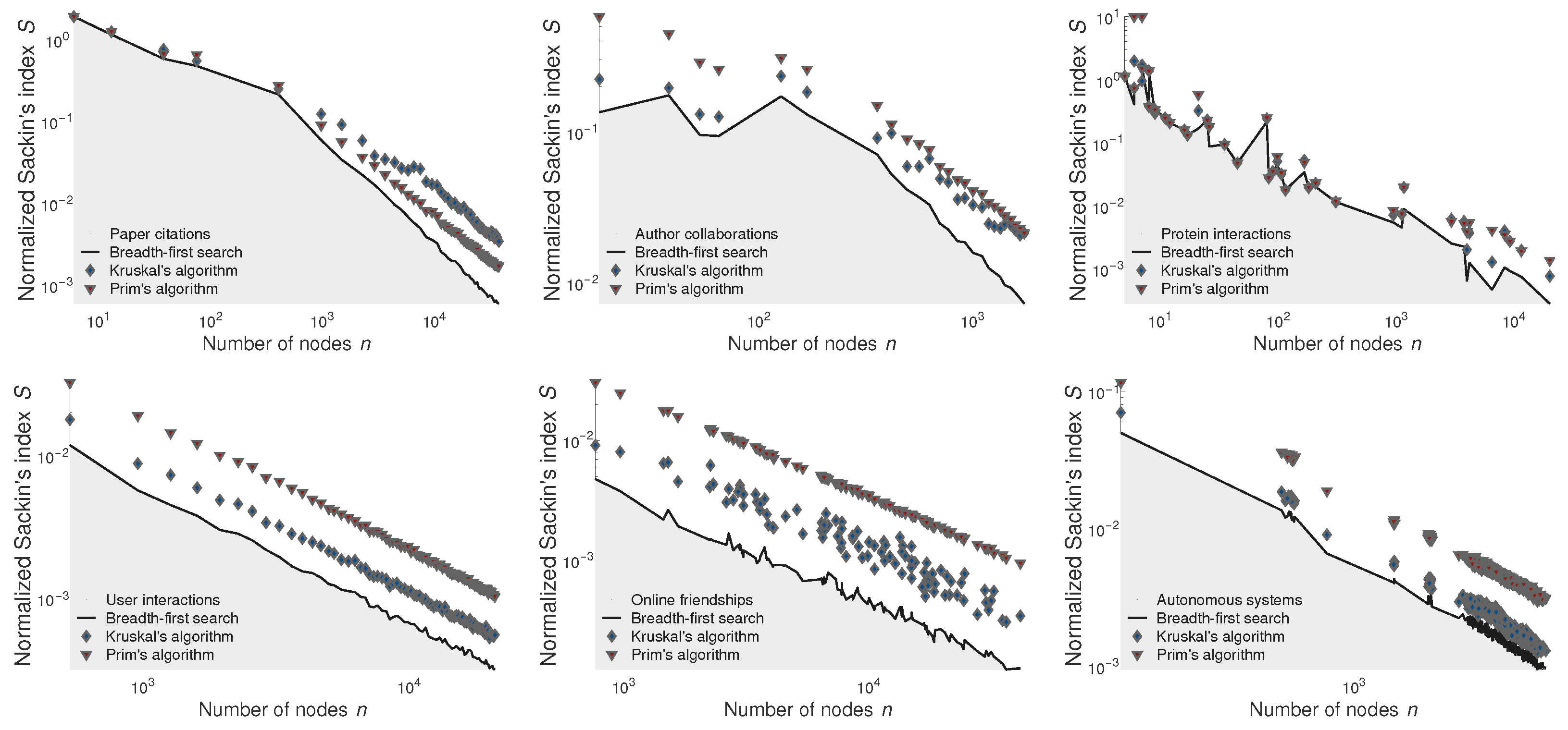
A well-balanced spanning tree would already imply short distances between the nodes $⟨d⟩\sim \log n$ and also the diameter $d_{\max }\sim \log n$. One of the most commonly used measures of tree balance is Sackin’s index of tree imbalance [25]. Figure 7 and Table 5 show normalized Sackin’s index S [32] of spanning trees computed with different algorithms. Notice that in all but a few cases, Sackin’s index S of spanning trees computed with the breadth-first search algorithm is strictly smaller than that of spanning trees computed with any other algorithm, often by an order of magnitude. Therefore, the breadth-first search algorithm computes the most balanced spanning trees. Another widely used measure of tree compactness or density [46] from the chemical graph theory literature is the so-called Wiener’s index [24]. Weiner’s index is defined as the unnormalized distance between all pairs of nodes $\left({\displaystyle \genfrac{}{}{0pt}{}{n}{2}}\right)⟨d⟩$ and thus can be readily observed in Figure 4.

Figure 7. Normalized Sackin’s index S of spanning trees computed with different algorithms. The plots show estimates over 25 realizations.

Table 5. The percentage of real networks for which normalized Sackin’s index S of spanning trees differs.

	Breadth-First Search vs. Prim’s alg.			Breadth-First Search vs. Kruskal’s alg.
Collection	${\mathbf{S}}^{\mathrm{B}}<{\mathbf{S}}^{\mathrm{P}}$	${\mathbf{S}}^{\mathrm{B}}={\mathbf{S}}^{\mathrm{P}}$	${\mathbf{S}}^{\mathrm{B}}>{\mathbf{S}}^{\mathrm{P}}$	${\mathbf{S}}^{\mathrm{B}}<{\mathbf{S}}^{\mathrm{K}}$	${\mathbf{S}}^{\mathrm{B}}={\mathbf{S}}^{\mathrm{K}}$	${\mathbf{S}}^{\mathrm{B}}>{\mathbf{S}}^{\mathrm{K}}$
Paper citations	$97.8\%$	$2.2\%$	$0.0\%$	$97.8\%$	$2.2\%$	$0.0\%$
Author collaborations	$100.0\%$	$0.0\%$	$0.0\%$	$100.0\%$	$0.0\%$	$0.0\%$
Protein interactions	$62.5\%$	$37.5\%$	$0.0\%$	$60.0\%$	$37.5\%$	$2.5\%$
User interactions	$100.0\%$	$0.0\%$	$0.0\%$	$100.0\%$	$0.0\%$	$0.0\%$
Online friendships	$100.0\%$	$0.0\%$	$0.0\%$	$100.0\%$	$0.0\%$	$0.0\%$
Autonomous systems	$100.0\%$	$0.0\%$	$0.0\%$	$100.0\%$	$0.0\%$	$0.0\%$

For a graphical representation of normalized Sackin’s index S of spanning trees, see Figure 7.

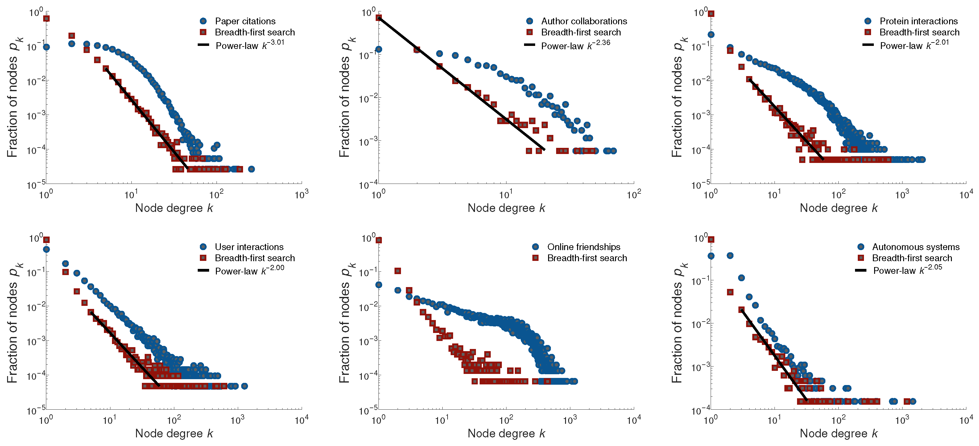
It is further interesting that the node degree distribution $p_k$ of the spanning trees computed with the breadth-first search algorithm often follows a power-law $p_k\sim k^{-\gamma }$ [47], regardless of whether the network is scale-free or not [43,48]. Figure 8 shows the node degree distribution $p_k$ of the largest networks in Table 1 and their spanning trees. Under the goodness-of-fit test at p-value = 0.1 [47], a  $p_k\sim k^{-\gamma }$ is a plausible fit of the degree distribution $p_k$ for the protein interactions and autonomous systems networks in the right column of Figure 8. On the other hand, the degree distribution $p_k$ of the spanning trees follows a power-law in all cases but the online friendships network, while the maximum likelihood estimates of the power-law exponents $\gamma$ are shown with solid lines in Figure 8. Considering the impact of a power-law degree distribution on network structure and dynamics, this property may be useful in practical applications of spanning trees.

Figure 8. Node degree distribution $p_k$ of real networks and their spanning trees computed with the breadth-first search algorithm. The power-law distributions are maximum likelihood estimates at p-value = 0.1 [47].

To summarize, we conclude that if a spanning tree should retain a short average distance between the nodes $⟨d⟩$ and a small diameter $d_{\max }$ of real networks, then the breadth-first search algorithm should be used. Whether preserving the distances is actually desired or favorable depends on a specific application, which we consider in the next section.

4. Applications

A spanning tree can be viewed as a technique for discovering a network backbone or skeleton [10,11], with applications in network visualization, node importance and link prediction. Moreover, a spanning tree is one of the basic approaches for network simplification or sampling [6,8]. Any computation that can be well approximated from a spanning tree of a network, without the need to apply an algorithm to the entire network, can provide computational benefits. In particular, many network applications require superlinear $\mathcal{O}\left(m\log n\right)$ or even quadratic algorithms $\mathcal{O}\left(mn\right)$, where n and m are the number of nodes and edges. These include community detection algorithms [49] and techniques for computing node importance or similarity [1]. In contrast, the computation of a spanning tree using the breadth-first search algorithm has a linear complexity $\mathcal{O}\left(m\right)$ and therefore does not contribute to the overall time complexity.

In this section, we consider two applications of spanning trees, where it is desired to preserve the distances between the nodes of a network.

4.1. Node Importance

Computing the importance of nodes in a network is a classical application of network science with various use cases. There exist many node measures or indices [50], which are known as measures of node position or centrality in the social network analysis literature [51,52]. The measure based on the distances between the nodes is called closeness centrality, which estimates the extent to which the node appears to be at the “center” of a network. This measure is often used in operations research and logistics. The closeness centrality of a node $i\in V$ in graph $G(V,E)$ can be defined as ${\displaystyle \frac{1}{n-1}}{\sum }_{j\ne i}{d}_{ij}^{-1}$ [52], where $n=\left|V\right|$ is the number of nodes and $d_{ij}$ is the distance between the nodes $i,j\in V$. The time complexity of computing closeness centrality of all nodes in a network is $\mathcal{O}\left(nm\right)$ and no more efficient algorithm exists [27].

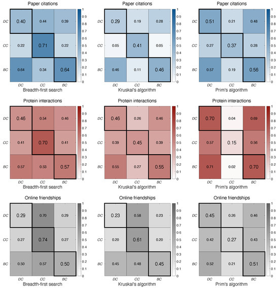
Figure 9 shows the Pearson correlation coefficient between node closeness centrality in real networks and their spanning trees computed with the breadth-first search, Kruskal’s and Prim’s algorithms. The coefficients for the breadth-first search algorithm are shown in the center of the heatmaps in the left column of Figure 9. These correlations are all $\ge$0.70, which indicates a strong linear correlation. On the other hand, the correlation coefficients for the spanning trees computed using Kruskal’s algorithm in the middle column and Prim’s algorithm in the right column are on average $0.49$ and $0.26$, respectively. Thus, in agreement with the previous results, the breadth-first search algorithm best preserves the distances between the nodes of real networks, not only on average but also at the level of individual nodes.

Figure 9. Pearson correlation coefficient between node centrality in real networks and their spanning trees computed with the breadth-first search (left), Kruskal’s (middle) and Prim’s (right) algorithms. The measures include node degree centrality $DC$, closeness centrality $CC$ and betweenness centrality $BC$, where the values are estimates over 25 realizations.

Merely for comparison, Figure 9 also shows the Pearson correlation coefficient for node degree centrality and betweenness centrality [51]. The latter measures the extent to which a node appears to serve as a “bridge” in a network and is defined as the proportion of all shortest paths between pairs of nodes that pass through a node. The time complexity of computing the betweenness centrality of all nodes in a network is again $\mathcal{O}\left(nm\right)$ [53].

4.2. Network Visualization

In addition to the computational benefits, a network simplification technique such as a spanning tree can also be useful for network visualization. Any visualization using a wiring diagram or other approach is limited in the size of a network it can represent and in the structural properties of a network it can reveal [54,55]. Classical algorithms for computing a layout of a network include force-directed algorithms [56,57] and algorithms that embed the nodes in a plane so that their Euclidean distance matches their network distance as closely as possible [58]. It is, therefore, important that a spanning tree preserves the distances between the nodes of a network if it is to be used with such visualization algorithms.

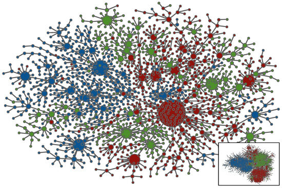
Figure 10 shows a wiring diagram of a spanning tree of the largest connected component of the SICRIS author collaboration network [34]. The spanning tree was computed with the breadth-first search algorithm. The wiring diagram illustrates how authors from the same discipline cluster in specific regions and how authors from different disciplines collaborate. In contrast, the visualization of the entire network is much more involved, only revealing three clusters (see inset of Figure 10), while providing very limited insight into the patterns of author collaboration [59]. Since there exists no generally accepted quantitative measure for the quality of network visualization, we refrain from further subjective interpretation.

Figure 10. Spanning tree of the SICRIS author collaboration network computed with the breadth-first search algorithm. The size of the nodes is proportional to their degree, while the colors represent primary author disciplines: natural sciences (red), engineering (green), medical sciences (blue) and others (gray). The inset shows a wiring diagram of the entire network. The layouts were computed with the Large Graph Layout algorithm [26].

5. Conclusions

A spanning tree is one of the most straightforward ways to network simplification or sampling, and to reveal its backbone or skeleton [8,10]. Well-known algorithms for computing a spanning tree of a weighted network are Prim’s and Kruskal’s algorithms [1,13]. However, when applied to unweighted networks, which are much more common in practice [20], these algorithms fail to capture the structural properties of real networks, such as short distances between the nodes and a small network diameter. Prior to this work, there existed no empirical evaluation or comparison of the algorithms on large-scale networks.

As we demonstrate in this paper, an algorithm based on the breadth-first search node traversal effectively retains the average and maximum distances in synthetic graphs and real networks, overall and at the level of individual nodes. The spanning trees are also well-balanced and highly compact, while the node degree distribution often follows a power-law. Besides being an effective approach for network sampling [18], spanning trees offer computational benefits in large-scale networks [60] and are crucial for practical applications in medical sciences [61], operations research [62], transportation and logistics [63], and communication in distributed systems [64]. Other applications include network visualization, where well-balanced spanning trees reduce clutter and highlight the network’s hierarchical structure [59]. Thus, if a spanning tree of an unweighted network is supposed to retain its structure, then the breadth-first search algorithm should be preferred to other algorithms.

We emphasize that the breadth-first search algorithm does not provide the correct result in weighted networks, where Prim’s algorithm or Kruskal’s algorithm should be used. Furthermore, a spanning tree is not the most suitable technique for simplifying a network in all applications. For instance, a convex skeleton [11] is a natural generalization of a spanning tree that also preserves local density, resulting in a high clustering coefficient and an emphasized community structure. Moreover, if one is interested in predicting the behavior of dynamical processes, then a high-salience skeleton [9] might be preferred.

Appendix A.1. Prim’s Algorithm

Prim’s algorithm for computing a spanning tree T of an undirected connected graph G operates as follows (see Algorithm A1). First, the algorithm selects a random seed node $i\in V_G$ from graph G and adds it to an empty tree T (lines 2, 3). The node i serves as a starting point for computing the spanning tree T. Then, on each step of the algorithm (lines 4–8), a random edge $\{i,j\}\in E_G$ from graph G is selected that leads from a node $i\in V_T$ already in the tree T to a node $j\notin V_T$ not yet in the tree T (line 5). Both node j and edge $\{i,j\}$ are added to the tree T (lines 6, 7). Finally, when there is no further node $i\in V_G$ in graph G such that node $i\notin V_T$ is not already in the tree T, the algorithm stops (line 4). At this point, the tree T is a spanning tree of graph G (line 9).

Algorithm A1 Prim’s algorithm

Require: undirected graph G Ensure: spanning tree T   1: $T\leftarrow$ empty graph   2: i ← Random$(i\in V_G)$                     ▹ Random seed node.   3: add node i to $V_T$                     ▹ Add selected seed node.   4: while $\exists i\in V_G:i\notin V_T$ do               ▹ There exists non-visited node?   5:        $\{i,j\}\leftarrow$ Random  $(\{i,j\}\in E_G:i\in V_T\wedge j\notin V_T)$       ▹ Edge to non-visited node.   6:        add node j to $V_T$                    ▹ Add non-visited node.   7:        add edge $\{i,j\}$ to $E_T$                      ▹ Add selected edge.   8: end while   9: return T

Prim’s algorithm is nondeterministic and can compute any spanning tree of a graph. The actual spanning tree depends on a random selection of the seed node (line 2) and on a random selection of the edges to expand the tree (line 5). The latter is most efficiently implemented by rejection sampling over an array list of edges to non-visited nodes. For simplicity, we do not make these computations explicit in Algorithm A1.

Assume that the graph is represented with an adjacency list. In the case of weighted graphs, the time complexity of Prim’s algorithm implemented with a Fibonacci heap is $\mathcal{O}(m+n\log n)$. For unweighted graphs, which we consider in this paper, the heap can be replaced by an array list, which reduces the time complexity to $\mathcal{O}\left(m\right)$.

Appendix A.2. Kruskal’s Algorithm

Kruskal’s algorithm turns out to be inefficient for our purposes in this paper, so we do not provide the exact pseudocode here. The algorithm is nondeterministic and can compute any spanning tree of a graph. The actual spanning tree depends on a random selection of the edges to merge the trees at each step. The time complexity of the algorithm using a disjoint-set data structure is $\mathcal{O}\left(m\log n\right)$, for either weighted or unweighted graphs.

Appendix A.3. Breadth-First Search

The breadth-first search algorithm for computing a spanning tree T of an undirected connected graph G operates as follows (see Algorithm A2). In contrast to before, we make all computations in Algorithm A2 explicit. First, the algorithm selects a random seed node $i\in V_G$ from graph G and adds it to an empty tree T (lines 3, 4). The node i is also added to an empty queue $Q\subseteq V_T$. Then, on each step of the algorithm (lines 5–11), a node $i\in Q$ is removed from the beginning of the queue Q (line 6) and all edges that lead from node $i\in V_T$ already in the tree T to nodes $j\notin V_T$ not yet in the tree T are processed (lines 7–10). All nodes j and edges $\{i,j\}$ are added to the tree T (lines 8, 9), while nodes j are also added to the queue Q for further processing. Finally, when there is no other node $i\in Q$ in the queue Q, the algorithm stops (line 5). At this point the tree T is a spanning tree of graph G (line 12).

Algorithm A2 Breadth-first search

Require: undirected graph G Ensure: spanning tree T   1: $T\leftarrow$ empty graph   2: $Q\leftarrow$ empty queue   3: i ← Random $(i\in V_G)$                        ▹ Random seed node.   4: add node i to $V_T$ and Q                     ▹ Add selected seed node.   5: while $\exists i\in Q$ do                    ▹ There exists non-processed node?   6:       $i\leftarrow$ remove node from Q                ▹ Select first non-processed node.   7:       for $\{i,j\}\in E_G:j\notin V_T$ do                  ▹ Edges to non-visited nodes.   8:             add node j to $V_T$ and Q                   ▹ Add non-visited node.   9:             add edge $\{i,j\}$ to $E_T$                       ▹ Add selected edge. 10:     end for 11: end while 12: return  T

The breadth-first search algorithm is nondeterministic and can again compute any spanning tree of a graph. The actual spanning tree depends on a random selection of the seed node (line 3) and the exact order in which the edges to expand the tree are processed (line 7). The time complexity of the algorithm using a queue of non-processed nodes is $\mathcal{O}\left(m\right)$, for either weighted or unweighted graphs.

References

- Newman, M.E.J. Networks, 2nd ed.; Oxford University Press: Oxford, UK, 2018. [Google Scholar]
- Tizzoni, M.; Bajardi, P.; Poletto, C.; Ramasco, J.J.; Balcan, D.; Gonçalves, B.; Perra, N.; Colizza, V.; Vespignani, A. Real-time numerical forecast of global epidemic spreading: Case study of 2009 A/H1N1pdm. BMC Med. 2012, 10, 165. [Google Scholar] [CrossRef] [Scilit]
- Zitnik, M.; Sosič, R.; Feldman, M.W.; Leskovec, J. Evolution of resilience in protein interactomes across the tree of life. Proc. Natl. Acad. Sci. USA 2019, 116, 4426–4433. [Google Scholar] [CrossRef] [Scilit]
- Fortunato, S.; Bergstrom, C.T.; Börner, K.; Evans, J.A.; Helbing, D.; Milojević, S.; Petersen, A.M.; Radicchi, F.; Sinatra, R.; Uzzi, B.; et al. Science of science. Science 2018, 359, eaao0185. [Google Scholar] [CrossRef] [Scilit] [PubMed]
- Backstrom, L.; Boldi, P.; Rosa, M.; Ugander, J.; Vigna, S. Four degrees of separation. In Proceedings of the ACM International Conference on Web Science, Evanston, IL, USA, 22–24 June 2012; pp. 45–54. [Google Scholar]
- Leskovec, J.; Faloutsos, C. Sampling from large graphs. In Proceedings of the ACM SIGKDD International Conference on Knowledge Discovery and Data Mining, Philadelphia, PA, USA, 20–23 August 2006; pp. 631–636. [Google Scholar]
- Hamann, M.; Lindner, G.; Meyerhenke, H.; Staudt, C.L.; Wagner, D. Structure-preserving sparsification methods for social networks. Soc. Netw. Anal. Min. 2016, 6, 22. [Google Scholar] [CrossRef] [Scilit]
- Blagus, N.; Šubelj, L.; Bajec, M. Empirical comparison of network sampling: How to choose the most appropriate method? Phys. A Stat. Mech. Its Appl. 2017, 477, 136–148. [Google Scholar] [CrossRef] [Scilit]
- Grady, D.; Thiemann, C.; Brockmann, D. Robust classification of salient links in complex networks. Nat. Commun. 2012, 3, 864. [Google Scholar] [CrossRef] [Scilit]
- Coscia, M.; Neffke, F. Network backboning with noisy data. In Proceedings of the IEEE International Conference on Data Engineering, San Diego, CA, USA, 19–22 April 2017; pp. 425–436. [Google Scholar]
- Šubelj, L. Convex skeletons of complex networks. J. R. Soc. Interface 2018, 15, 20180422. [Google Scholar] [CrossRef] [Scilit]
- Simas, T.; Correia, R.B.; Rocha, L.M. The distance backbone of complex networks. J. Complex Netw. 2021, 9, cnab021. [Google Scholar] [CrossRef] [Scilit]
- Bollobás, B. Modern Graph Theory; Springer: Berlin/Heidelberg, Germany, 1998. [Google Scholar]
- Pop, P.C. The generalized minimum spanning tree problem: An overview of formulations, solution procedures and latest advances. Eur. J. Oper. Res. 2020, 283, 1–15. [Google Scholar] [CrossRef] [Scilit]
- Diggans, C.T.; Bollt, E.M.; Ben-Avraham, D. Spanning trees of recursive scale-free graphs. Phys. Rev. E 2022, 105, 024312. [Google Scholar] [CrossRef] [Scilit]
- Henke, L.; Mehta, D. C-RST: A parallel algorithm for random spanning trees in network analytics. Appl. Netw. Sci. 2024, 9, 45. [Google Scholar] [CrossRef] [Scilit]
- Dhouib, S. Innovative method to solve the minimum spanning tree problem: The Dhouib-Matrix-MSTP (DM-MSTP). Results Control Optim. 2024, 14, 100359. [Google Scholar] [CrossRef] [Scilit]
- Rezvanian, A.; Vahidipour, S.M.; Jalali, Z.S. A spanning tree approach to social network sampling with degree constraints. Soc. Netw. Anal. Min. 2024, 14, 101. [Google Scholar] [CrossRef] [Scilit]
- Amure, R.; Agarwal, N.A. A comparative evaluation of social network analysis tools: Performance and community engagement perspectives. Soc. Netw. Anal. Min. 2025, 15, 100359. [Google Scholar] [CrossRef] [Scilit]
- Abdallah, S. Generalizing unweighted network measures to capture the focus in interactions. Soc. Netw. Anal. Min. 2011, 1, 255–269. [Google Scholar] [CrossRef] [Scilit]
- Bourgain, J. On Lipschitz embedding of finite metric spaces in Hilbert space. Isr. J. Math. 1985, 52, 46–52. [Google Scholar] [CrossRef] [Scilit]
- Watts, D.J.; Strogatz, S.H. Collective dynamics of ’small-world’ networks. Nature 1998, 393, 440–442. [Google Scholar] [CrossRef] [Scilit]
- Newman, M.E.J. The structure and function of complex networks. SIAM Rev. 2003, 45, 167–256. [Google Scholar] [CrossRef] [Scilit]
- Wiener, H. Structural determination of paraffin boiling points. J. Am. Chem. Soc. 1947, 69, 17–20. [Google Scholar] [CrossRef] [Scilit]
- Sackin, M.J. “Good” and “bad” phenograms. Syst. Biol. 1972, 21, 225–226. [Google Scholar] [CrossRef] [Scilit]
- Adai, A.T.; Date, S.V.; Wieland, S.; Marcotte, E.M. LGL: Creating a map of protein function with an algorithm for visualizing very large biological networks. J. Mol. Biol. 2004, 340, 179–190. [Google Scholar] [CrossRef] [Scilit]
- Knuth, D.E. The Art of Computer Programming; Addison-Wesley Professional: Amsterdam, The Netherlands, 2011. [Google Scholar]
- Rényi, A.; Szekeres, G. On the height of trees. J. Aust. Math. Soc. 1967, 7, 497–507. [Google Scholar] [CrossRef] [Scilit]
- Meir, A.; Moon, J.W. The distance between points in random trees. J. Comb. Theory 1970, 8, 99–103. [Google Scholar] [CrossRef] [Scilit]
- Fischer, M.; Herbst, L.; Kersting, S.A.; Kühn, L.; Wicke, K. Tree Balance Indices: A Comprehensive Survey, 1st ed.; Springer: Cham, The Netherlands, 2023. [Google Scholar]
- Lemant, J.; Le Sueur, C.; Manojlović, V.; Noble, R. Robust, universal tree balance indices. Syst. Biol. 2022, 71, 1210–1224. [Google Scholar] [CrossRef] [Scilit]
- Shao, K.T.; Sokal, R.R. Tree balance. Syst. Zool. 1990, 39, 266–276. [Google Scholar] [CrossRef] [Scilit]
- American Physical Society. APS Dataset. 2015. Available online: http://journals.aps.org/datasets (accessed on 1 October 2025).
- Institute of Information Science. SICRIS Database. 2010. Available online: http://www.sicris.si (accessed on 1 October 2025).
- Stark, C.; Breitkreutz, B.J.; Reguly, T.; Boucher, L.; Breitkreutz, A.; Tyers, M. BioGRID: A general repository for interaction datasets. Nucleic Acids Res. 2006, 34, 535–539. [Google Scholar] [CrossRef] [Scilit]
- Biological General Repository for Interaction Datasets. BioGRID Database. 2016. Available online: http://thebiogrid.org (accessed on 1 October 2025).
- Paranjape, A.; Benson, A.R.; Leskovec, J. Motifs in temporal networks. In Proceedings of the ACM International Conference on Web Search and Data Mining, Cambridge, UK, 6–10 February 2017; pp. 601–610. [Google Scholar]
- Leskovec, J.; Krevl, A. SNAP Datasets. 2014. Available online: http://snap.stanford.edu/data (accessed on 1 October 2025).
- Traud, A.L.; Mucha, P.J.; Porter, M.A. Social structure of Facebook networks. Phys. A Stat. Mech. Its Appl. 2012, 391, 4165–4180. [Google Scholar] [CrossRef] [Scilit]
- Rossi, R.A.; Ahmed, N.K. Network Data Repository. 2015. Available online: http://networkrepository.com (accessed on 1 October 2025).
- Leskovec, J.; Kleinberg, J.; Faloutsos, C. Graphs over time: Densification laws, shrinking diameters and possible explanations. In Proceedings of the ACM SIGKDD International Conference on Knowledge Discovery and Data Mining, Chicago, IL, USA, 21–24 August 2005; pp. 177–187. [Google Scholar]
- Erdős, P.; Rényi, A. On random graphs I. Publ. Math. Debr. 1959, 6, 290–297. [Google Scholar] [CrossRef] [Scilit]
- Barabási, A.L.; Albert, R. Emergence of scaling in random networks. Science 1999, 286, 509–512. [Google Scholar] [CrossRef] [Scilit]
- Cohen, R.; Havlin, S. Scale-free networks are ultrasmall. Phys. Rev. Lett. 2003, 90, 058701. [Google Scholar] [CrossRef] [Scilit]
- Barabási, A.L. Network Science; Cambridge University Press: Cambridge, UK, 2016. [Google Scholar]
- Ozen, M.; Lesaja, G.; Wang, H. Globally optimal dense and sparse spanning trees, and their applications. Stat. Optim. Inf. Comput. 2020, 8, 328–345. [Google Scholar] [CrossRef] [Scilit]
- Clauset, A.; Shalizi, C.R.; Newman, M.E.J. Power-law distributions in empirical data. SIAM Rev. 2009, 51, 661–703. [Google Scholar] [CrossRef] [Scilit]
- Broido, A.D.; Clauset, A. Scale-free networks are rare. Nat. Commun. 2019, 10, 1017. [Google Scholar] [CrossRef] [Scilit]
- Fortunato, S.; Hric, D. Community detection in networks: A user guide. Phys. Rep. 2016, 659, 1–44. [Google Scholar] [CrossRef] [Scilit]
- Schoch, D.; Brandes, U. Re-conceptualizing centrality in social networks. Eur. J. Appl. Math. 2016, 27, 971–985. [Google Scholar] [CrossRef] [Scilit]
- Freeman, L. A set of measures of centrality based on betweenness. Sociometry 1977, 40, 35–41. [Google Scholar] [CrossRef] [Scilit]
- Freeman, L.C. Centrality in social networks: Conceptual clarification. Soc. Netw. 1979, 1, 215–239. [Google Scholar] [CrossRef] [Scilit]
- Brandes, U. A faster algorithm for betweenness centrality. J. Math. Sociol. 2001, 25, 163–177. [Google Scholar] [CrossRef] [Scilit]
- Ma, K.L.; Muelder, C.W. Large-scale graph visualization and analytics. Computer 2013, 46, 39–46. [Google Scholar] [CrossRef] [Scilit]
- Gibson, H.; Faith, J.; Vickers, P. A survey of two-dimensional graph layout techniques for information visualisation. Inf. Vis. 2013, 12, 324–357. [Google Scholar] [CrossRef] [Scilit]
- Eades, P. A heuristic for graph drawing. Congr. Numer. 1984, 42, 149–160. [Google Scholar]
- Fruchterman, T.M.J.; Reingold, E.M. Graph drawing by force-directed placement. Softw. Pract. Exp. 1991, 21, 1129–1164. [Google Scholar] [CrossRef] [Scilit]
- Kamada, T.; Kawai, S. An algorithm for drawing general undirected graphs. Inf. Process. Lett. 1989, 31, 7–15. [Google Scholar] [CrossRef] [Scilit]
- Šubelj, L.; Fiala, D.; Ciglarič, T.; Kronegger, L. Convexity in scientific collaboration networks. J. Inf. 2019, 13, 10–31. [Google Scholar] [CrossRef] [Scilit]
- Kalyagin, V.A.; Pardalos, P.M.; Prokopyev, O.; Utkina, I. Computational Aspects and Applications in Large-Scale Networks, 1st ed.; Springer: Cham, Switzerland, 2017. [Google Scholar]
- Blomsma, N.; de Rooy, B.; Gerritse, F.; van der Spek, R.; Tewarie, P.; Hillebrand, A.; Otte, W.M.; Stam, C.J.; van Dellen, E. Minimum spanning tree analysis of brain networks: A systematic review of network size effects, sensitivity for neuropsychiatric pathology, and disorder specificity. Netw. Neurosci. 2022, 6, 301–319. [Google Scholar] [CrossRef] [Scilit]
- Hosseini, A. Uncertainty modeling and stability assessment of minimum spanning trees in network design. Mathematics 2024, 12, 3812. [Google Scholar] [CrossRef] [Scilit]
- Strzelczyk, A.; Guze, S. An approach to the analysis of critical elements of transport and logistics networks using graph theory. Int. J. Mar. Navig. Saf. Sea Transp. 2024, 18, 535–544. [Google Scholar] [CrossRef] [Scilit]
- Augustine, J.; Gilbert, S.; Kuhn, F.; Robinson, P.; Sourav, S. Latency, capacity, and distributed minimum spanning trees. J. Parallel Distrib. Comput. 2022, 126, 1–20. [Google Scholar] [CrossRef] [Scilit]
Disclaimer/Publisher’s Note: The statements, opinions and data contained in all publications are solely those of the individual author(s) and contributor(s) and not of MDPI and/or the editor(s). MDPI and/or the editor(s) disclaim responsibility for any injury to people or property resulting from any ideas, methods, instructions or products referred to in the content. |
© 2025 by the author. Licensee MDPI, Basel, Switzerland. This article is an open access article distributed under the terms and conditions of the Creative Commons Attribution (CC BY) license (https://creativecommons.org/licenses/by/4.0/).