


Abstract
The theory of fractional thermoelasticity is based on the fractional heat conduction equation. In the present paper, we consider an axisymmetric problem for an infinite solid with a penny-shaped crack of radius R under the prescribed temperature at its surfaces in the framework of fractional thermoelasticity. When the heat flux boundary conditions at the crack surfaces are assumed, the temperature field is determined directly from the heat conduction equation, whereas in the case of temperature prescribed at the crack surfaces, the boundary conditions are mixed, the problem is more complicated, and the temperature field is found from the corresponding dual integral equations. The important fracture characteristics—the stress intensity factor—is calculated in terms of the Wright function. The time-dependence of the stress intensity factor is presented for different values of the order of fractional derivative.
1. Introduction
The classical theory of heat conduction is grounded in the Fourier law [1,2,3]. Many theoretical and experimental results show that in materials with complex internal structure the Fourier law and the parabolic heat conduction equation resulting from this law do not describe the heat process in an appropriate way. This circumstance causes the appearance of nonclassical theories based on the generalized heat conduction equation (see, for example, [4,5,6,7,8,9,10,11,12,13,14]).
The generalized Fourier law [8,15,16] expressed in terms of integrals and derivatives of fractional order leads to the time-fractional heat conduction equation
with the Caputo derivative [17,18,19]
where is the gamma function. Integrating by parts the integral in the definition (2) and assuming that the function has continuous bounded derivatives, we obtain
(see § 2.4.1 in the book by Podlubny [17] and the proof of Theorem 2.1 in the book by Kilbas et al. [18]). Formula (3) explains the piecewise interpretation of the Caputo derivative and allows us to consider the limiting cases of the obtained results for integer orders of the derivative. The Caputo derivative has significant advantage compared to other definitions of fractional derivatives as its Laplace transform rule requires the knowledge of the initial values of the function and derivatives of the integer order. This feature permits us to formulate the problems involving the Caputo fractional derivative under initial conditions with well-known physical interpretations, in contrast to the Riemann-Liouville fractional derivative.
The Duhamel–Neumann equation [20,21]
is fundamental for the thermoelasticity theory. It asserts that the stress tensor depends not only on the strain tensor but also on the temperature T. Here and are Lamé constants, the bulk modulus is expressed as , denotes the thermal coefficient of volumetric expansion, is the unit tensor.
In the classical thermoelasticity, the temperature field T is determined from the standard heat conduction equation. Each generalization of the heat conduction equation generates the associated theory of thermal stresses. For example, Green and Naghdi [22] developed thermoelasticity without energy dissipation grounded in the wave equation for temperature, Lord and Shulman [23] proposed the generalized thermoelasticity associated with the Cattaneo telegraph equation for temperature; additional references can be also found in [24,25,26,27]. Fractional thermoelasticity grounded in Equation (1) was formulated in [15] and developed in many subsequent publications; the book [28] summarizes investigations in this area (see also the review papers [29,30,31]).
Strength of solids hinges essentially on existence of different types of cracks, slits and cuts inside a material. Sudden cooling of a material can lead to thermal shock and appearing of very large thermal stresses near such defects. Pivotal papers [32,33] initiated the investigation of thermoelastic problems for solids with cracks. Later on, this subject was widely studied in the literature in the framework of classical thermoelasticity [34,35,36,37,38,39] as well as in the content of generalized theories [40,41,42,43,44,45,46].
Cracks in the framework of fractional thermoelasticity were studied in [47,48,49,50,51] under the heat flux impact. It should be emphasized that the thermoelasticity problems for cracks with the temperature prescribed at their surfaces are more complicated than problems with the heat flux specified at the crack boundaries. When the heat flux boundary conditions at the crack surfaces are assumed, the temperature field is determined directly from the heat conduction equation, whereas in the case of temperature prescribed at the crack surfaces, the boundary conditions are mixed, and the temperature field should be found from dual integral equations. The novelty of this work compared with previous studies on penny-shaped cracks in fractional thermoelasticity consist in considering the boundary conditions with the prescribed temperature at the crack surfaces. The stress intensity factor is calculated in terms of the Wright function. The influence of the order of time-fractional derivative on the stress intensity factor is investigated.
2. The Temperature Field
We consider an axisymmetric problem for an infinite space , with a penny-shaped crack of radius R located in the plane . Our study is confined to the case symmetrical with respect to the plane . Hence, only the domain can be considered, and the temperature satisfies the time-fractional heat conduction equation
under zero initial conditions
The mixed boundary conditions are imposed:
The parameter shows which part of the crack surface is heated.
In what follows, we assume that . The Laplace transform with respect to time t and the Hankel transform with respect to the radial coordinate r applied to the heat conduction Equation (5) lead to the equation
having the solution satisfying the zero condition at infinity
Here the asterisk denotes the Laplace transform, the hat marks the Hankel transform, s is the Laplace transform variable, is the Hankel transform variable.
After inverting the Hankel transform, we get
It is convenient to introduce new unknown function
and rewrite the dual integral Equations (13) and (14) as
The solution of the dual integral Equations (16) and (17) is represented as
where is an auxiliary function and is some constant.
In this case, due to the Weber discontinuous integral [52]
the second dual integral Equation (17) is satisfied identically, and from Equation (16) we obtain
Differentiation of Equation (20) with respect to the radial coordinate r gives
Next we use the approximation
In the case of classical heat conduction (), the idea of such an approximation was suggested by Kudryavtsev and Parton [53] and later on used in many publications (see, for example, [35,37,54,55]). Kudryavtsev and Parton [53] and Parton [54] analyzed the approximation
for different values of the parameter b, carried out the numerical estimation and graphical interpretation of this approximation and showed that the best choice is which is used in Equation (22) (see Figure 1 and Figure 2 in the paper by Kudryavtsev and Parton [53] and Figure 2 in the paper by Parton [54]). Such a choice can also be substantiated by the expansion of the corresponding square root function into a Maclaurin series. Additional substantiation of the approximation (22) is provided by the identical limits
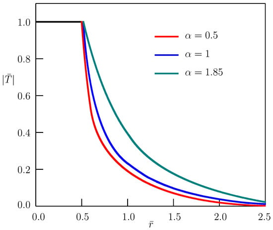
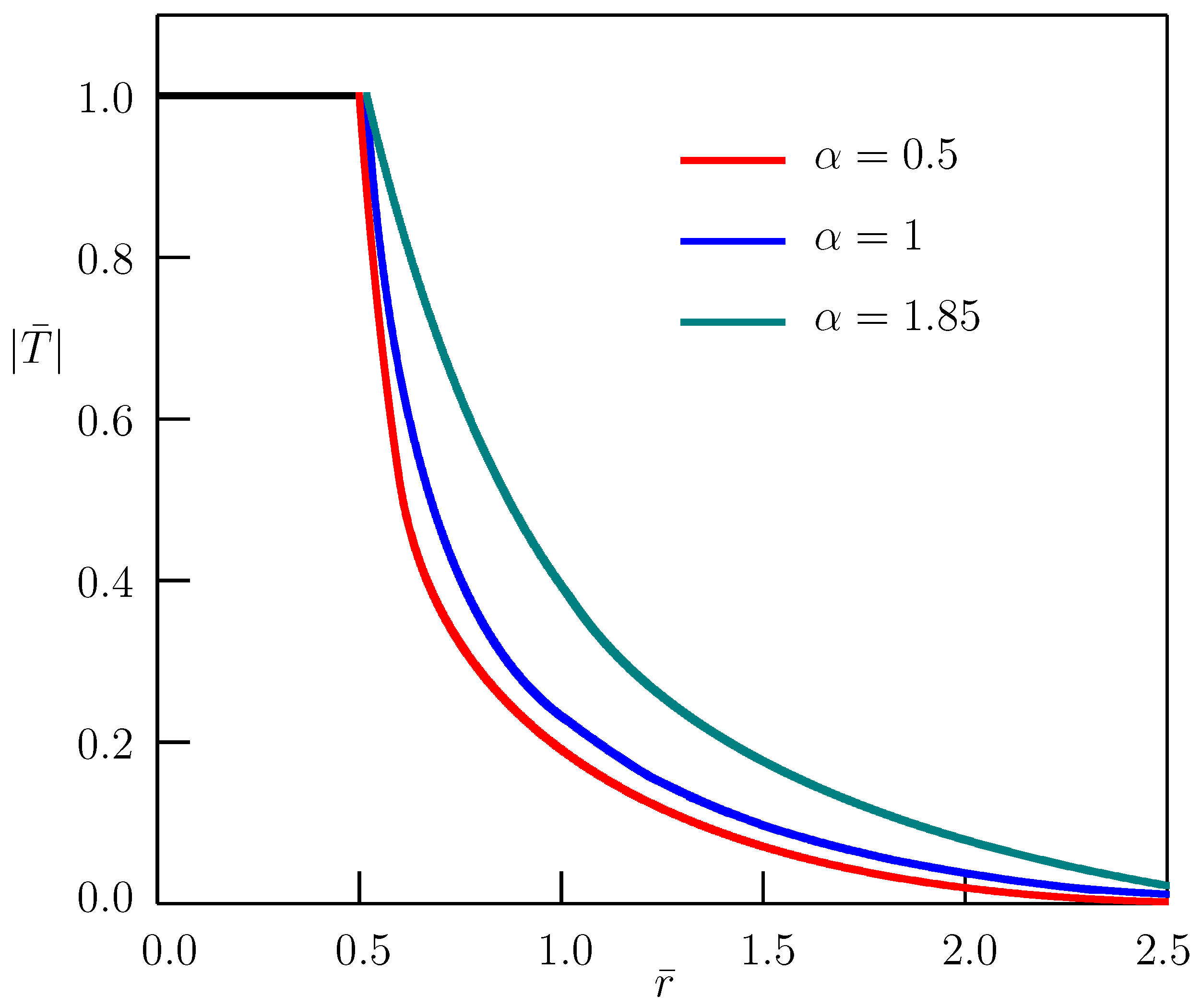
Figure 1.
Temperature dependence on distance; , .
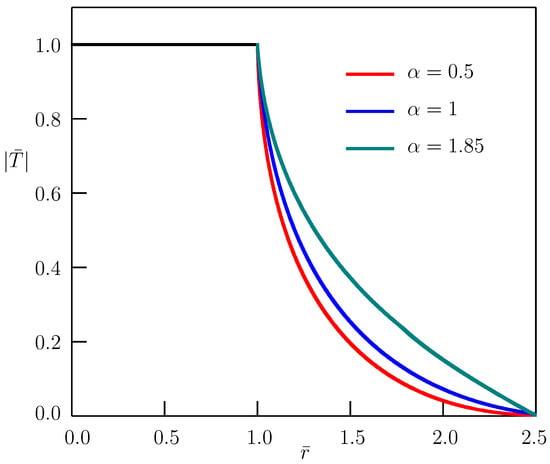
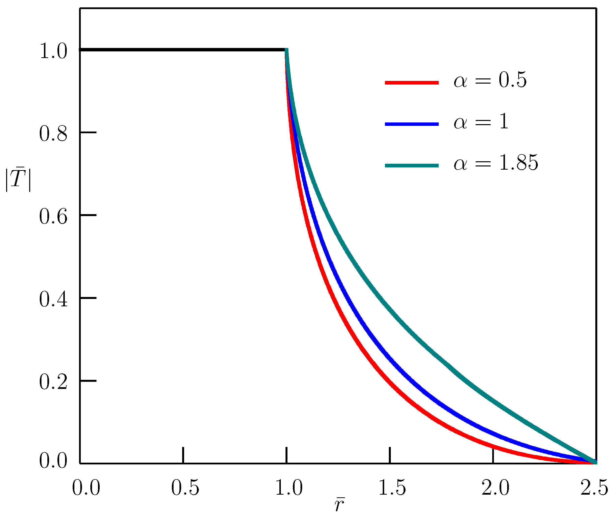
Figure 2.
Temperature dependence on distance; , .
Accounting for the approximation (22) in Equation (21) and utilizing the integral [52]
we arrive at the equation
where
Interpreting Equation (27) as a Schlömilch equation, its solution can be written as [56]
Using integral (A1) presented in Appendix A, from Equations (28) and (29) we obtain:
or
Integral (A2) from Appendix A allows us to reduce Equation (31) to the following expression for the function :
where the notation
is introduced.
From the first dual integral Equation (16), within the accepted approximation accounting for integrals (A3)–(A5) from Appendix A, we obtain
It follows from Equation (10) that
where
Hence
In particular, for
It is important that according to equations (A3) and (A4) from Appendix A, the second integral in Equation (40) equals zero for , and from Equation (A5) it follows that the boundary condition (7) is fulfilled. In such a way, we get
Due to the following formula for the inverse Laplace transform [17,18]
where is the Mittag-Leffler function in two parameters
we arrive at
In the particular case , taking into account the necessary equations for the inversion of the Laplace transform [57], we obtain
where is the error function of an imaginary argument.
Figure 1 and Figure 2 show the temperature dependence on distance r for and different values of the order of fractional derivative and the parameter . The following nondimensional quantities are introduced:
For integrals over the semi-infinite domain used for evaluations in Figure 1 and Figure 2, we truncate the domain to . Next we divide this domain into smaller subintervals and apply Gauss-Legendre quadrature in each subdomain with tolerance .
Now we return to Equation (39). To obtain the analytical solution for the temperature field , we apply to Equation (39) the Fourier cosine transform, use the approximation (22), and after some mathematical treatment we receive
The temperature field for the classical heat conduction () reads:
3. The Stress Intensity Factor
To investigate the stressed state of a solid caused by the temperature field , the displacement potential [58,59] is usually employed. In cylindrical coordinates in the case of axial symmetry, the displacement potential is found from the equation
and the components of the stress tensor are written as
The total stress field consists of two parts: the stress caused by the temperature field T and the stress required to satisfy the corresponding mechanical boundary conditions
Accounting for Equation (37) and applying the Laplace and Hankel integral transforms to Equation (52), we obtain the differential equation
Assuming , which allows us to satisfy the boundary condition for (see Equations (56) and (58)), we also evaluate the coefficient M:
In this paper, we restrict ourselves to calculation of the most important fracture characteristics—the stress intensity factor which is expressed as [60]
It follows from Equation (55) that
Equations (61)–(63) with taking into account Equations (22) and (38) give
Substituting the expression (66) into Equation (64) and evaluating the integral with respect to r (see Equation (A6) from Appendix A), we obtain
Next we use the necessary trigonometric identities and evaluate the appearing integrals according to Equations (A2), (A7) and (A8) from Appendix A. In the Laplace transform domain, we get
Inversion of the Laplace transform accounting for the following formula [61]
where is the Wright function [17,18,62]
results in the final expression for the stress intensity factor
We have used the approximation sign in Equation (71) to emphasize that this equation is obtained under the approximation (22).
The analogous equation for the classical thermoelasticity with the standard heat conduction equation () reads
where is the complementary error function.
Another particular case of Equation (71) corresponds to thermoelasticity without energy dissipation proposed by Green and Naghdi [22] based on the wave equation for temperature ():
where is the Heaviside step function.
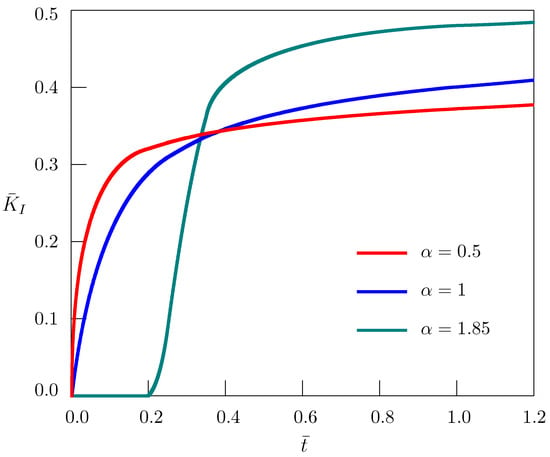
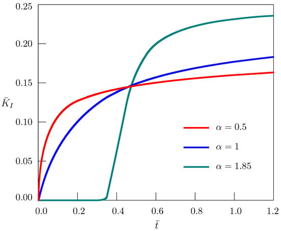
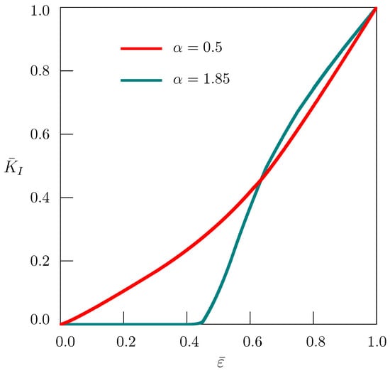
The nondimensional stress intensity factor
is shown in Figure 3, Figure 4 and Figure 5 for different values of the order of fractional derivative.
Figure 3.
Dependence of stress intensity factor on time; .
Figure 4.
Dependence of stress intensity factor on time; .
Figure 5.
Dependence of stress intensity factor on parameter ; .
4. Concluding Remarks
The classical thermoelasticity is associated with the parabolic heat conduction equation, whereas the fractional thermoelasticity is based on the time-fractional heat conduction equation with the Caputo derivative of the order . For , the fractional heat conduction equation interpolates between the localized heat conduction based on the elliptic Helmholtz equation for temperature () and the parabolic heat conduction (). In this case, the fractional thermoelasticity interpolates between the localized and standard thermoelasticity. For , the fractional heat conduction equation interpolates between the parabolic heat conduction () and ballistic heat conduction based on the wave equation for temperature (). In this instance, the fractional thermoelasticity interpolates between the standard thermoelasticity and thermoelasticity without energy dissipation. The fractional thermoelasticity permits better description of behavior of materials with complex internal structure, especially when a solid contains different types od defects.
We have studied the axisymmetric time fractional heat conduction equation with the Caputo derivative of the order in an infinite space containing a penny-shaped crack under the prescribed temperature at a part of its surfaces. The parameter describes which part of the crack surface is heated. The temperature field is obtained in the form of integrals expressed in terms of Mittag-Leffler functions. For numerical calculation of the Mittag-Leffler function, the algorithm proposed in [63] was employed. For real values of argument, this algorithm ensures a numerical accuracy of the order .
The displacement potential was used for investigation of the stressed state of a solid, in particular for studying the stress intensity factor which was obtained in terms of the Wright function. Numerical evaluation of the Wright function was carried out using the algorithm elaborated in [64]. According to [65], a numerical accuracy of this algorithm is between and .
The limitation of the present study consists in difficulty of obtaining analytical solution of dual integral equations for temperature, especially for more complicating heating of the crack surfaces. Another limitation is connected with the use of quasistatic thermoelasticity. We assume that the time of thermal disturbance spreading through a body is longer than the time of acoustic wave travel and neglect the inertial term in equation of motion. Such an assumption may not be valid for oscillating heating of the crack surfaces. We intend to address these aspects in future research.
It is important that for the stress intensity factor does not depend on the order of fractional derivative, but for such a dependence becomes crucial. At small values of time, the stress intensity factor is larger for lower orders of fractional derivative, but for large values of time the situation is inverse. When approaches 2, it is evident from Figure 3 and Figure 4 how the associated stress intensity factor approaches the corresponding Heaviside function appearing in Equation (73). In terms of nondimensional quantities, such a Heaviside function corresponds to the wave front at the point .
Author Contributions
Conceptualization, Y.P. and T.K.; methodology, Y.P. and T.K.; validation, T.K. and A.Y.; formal analysis, A.Y.; investigation, Y.P., T.K. and A.Y.; software, T.K. and A.Y.; supervision, Y.P.; writing—original draft preparation, T.K. and A.Y.; writing—review and editing, Y.P. All authors have read and agreed to the published version of the manuscript.
Funding
This research received no external funding.
Institutional Review Board Statement
Not applicable.
Informed Consent Statement
Not applicable.
Data Availability Statement
The original contributions presented in this study are included in the article. Further inquiries can be directed to the corresponding author.
Conflicts of Interest
The authors declare no conflicts of interest.
Appendix A. Integrals
The following integrals [52,66] are used in the paper
References
- Fourier, J.-B.-J. Théorie Analytique de la Chaleur; Firmin Didot: Paris, France, 1822. [Google Scholar]
- Friedman, R.M. The creation of a new science: Joseph Fourier’s analytical theory of heat. Hist. Stud. Phys. Sci. 1977, 8, 73–99. [Google Scholar] [CrossRef] [Scilit]
- Narasimhan, T.N. Fourier’s heat conduction equation: History, influences and connections. Rev. Geophys. 1999, 37, 151–172. [Google Scholar] [CrossRef] [Scilit]
- Joseph, D.D.; Presiosi, L. Heat waves. Rev. Mod. Phys. 1989, 61, 41–73. [Google Scholar] [CrossRef] [Scilit]
- Sobolev, S.L. Equations of transfer in non-local media. Int. J. Heat Mass Transf. 1994, 37, 2175–2182. [Google Scholar] [CrossRef] [Scilit]
- Wang, L.; Zhou, X.; Wei, X. Heat Conduction: Mathematical Models and Analytical Solutions; Springer: Berlin, Germany, 2008. [Google Scholar]
- Straughan, B. Heat Waves; Springer: New York, NY, USA, 2011. [Google Scholar]
- Povstenko, Y. Linear Fractional Diffusion-Wave Equation for Scientists and Engineers; Birkhäuser: New York, NY, USA, 2015. [Google Scholar]
- Tzou, D.Y. Macro- to Microscale Heat Transfer: The Lagging Behavior, 2nd ed.; John Wiley: Chichester, UK, 2015. [Google Scholar]
- Suzuki, A.; Fomin, S.A.; Chugunov, V.A.; Niibori, Y.; Hashida, T. Fractional diffusion modeling of heat transfer in porous and fractured media. Int. J. Heat Mass Transf. 2016, 103, 611–618. [Google Scholar] [CrossRef] [Scilit]
- Evangelista, L.R.; Lenzi, E.K. Fractional Diffusion Equations and Anomalous Diffusion; Cambridge University Press: Cambridge, UK, 2018. [Google Scholar]
- Zhang, Z.M. Nano/Microscale Heat Transfer, 2nd ed.; Springer: Cham, Switzerland, 2020. [Google Scholar]
- Sobolev, S.L.; Dai, W. Heat transport on ultrashort time and space scales in nanosized systems: Diffusive or wave-like? Materials 2022, 15, 4287. [Google Scholar] [CrossRef] [Scilit]
- Zhmakin, A.I. Non-Fourier Heat Conduction: From Phase-Lag Models to Relativistic and Quantum Transport; Springer: Cham, Switzerland, 2023. [Google Scholar]
- Povstenko, Y. Fractional heat conduction equation and associated thermal stresses. J. Therm. Stresses 2005, 28, 83–102. [Google Scholar] [CrossRef] [Scilit]
- Povstenko, Y. Thermoelasticity that uses fractional heat conduction equation. J. Math. Sci. 2009, 162, 296–305. [Google Scholar] [CrossRef] [Scilit]
- Podlubny, I. Fractional Differential Equations; Academic Press: San Diego, CA, USA, 1999. [Google Scholar]
- Kilbas, A.A.; Srivastava, H.M.; Trujillo, J.J. Theory and Applications of Fractional Differential Equations; Elsevier: Amsterdam, The Netherlands, 2006. [Google Scholar]
- Li, C.P.; Zeng, F.H. Numerical Methods for Fractional Calculus; Chapman and Hall/CRC: Boca Raton, FL, USA, 2015. [Google Scholar]
- Duhamel, J.-M.-C. Second mémoire sur les phénome`nes thermo-mécanique. J. Ec. Polytechn. 1837, 15, 1–57. [Google Scholar]
- Neumann, F. Vorlesung Über Die Theorie des Elasticität des Festen Körper und des Lichtäthers; Teubner: Leipzig, Germany, 1885. [Google Scholar]
- Green, A.E.; Naghdi, P.M. Thermoelasticity without energy dissipation. J. Elast. 1993, 31, 189–208. [Google Scholar] [CrossRef] [Scilit]
- Lord, H.W.; Shulman, Y. A generalized dynamical theory of thermoelasticity. J. Mech. Phys. Solids 1967, 15, 299–309. [Google Scholar] [CrossRef] [Scilit]
- Chandrasekharaiah, D.S. Thermoelasticity with second sound: A review. Appl. Mech. Rev. 1986, 39, 355–376. [Google Scholar] [CrossRef] [Scilit]
- Chandrasekharaiah, D.S. Hiperbolic thermoelasticity: A review of recent literature. Appl. Mech. Rev. 1998, 51, 705–729. [Google Scholar] [CrossRef] [Scilit]
- Hetnarski, R.B.; Eslami, M.R. Thermal Stresses—Advanced Theory and Applications; Springer: New York, NY, USA, 2009. [Google Scholar]
- Ignaczak, J.; Ostoja-Starzewski, M. Thermoelasticity with Finite Wave Speeds; Oxford University Press: Oxford, UK, 2009. [Google Scholar]
- Povstenko, Y. Fractional Thermoelasticity, 2nd ed.; Springer: Cham, Switzerland, 2024. [Google Scholar]
- Sheoran, S.S.; Kundu, P. Fractional order generalized thermoelasticity theories: A review. Int. J. Adv. Appl. Math. Mech. 2016, 3, 76–81. [Google Scholar]
- Povstenko, Y. Thermodiffusion in a deformable solid: Fractional calculus approach. In Handbook of Fractional Calculus with Applications, Volume 4: Applications in Physics, Part A; De Gruyter: Berlin, Germany, 2019; pp. 221–239. [Google Scholar]
- Khavale, S.G.; Gaikwad, K.R. Fractional thermoelasticity: A review. Easy Chair 2023, 3, 1–9. [Google Scholar] [CrossRef] [Scilit]
- Olesiak, Z.; Sneddon, I.N. The distribution of thermal stress in an infinite elastic solid containing a penny-shaped crack. Arch. Ration. Mech. Anal. 1959, 4, 238–254. [Google Scholar] [CrossRef] [Scilit]
- Florence, A.L.; Goodier, J.N. The linear thermoelastic problem of uniform heat flow disturbed by a penny-shaped insulated crack. Int. J. Eng. Sci. 1963, 1, 533–540. [Google Scholar] [CrossRef] [Scilit]
- Noda, N.; Matsunaga, Y. Transient thermoelastic problem in an infinite body containing a penny-shaped crack due to time and position dependent temperature condition. Z. Angew. Math. Mech. 1986, 66, 233–239. [Google Scholar] [CrossRef] [Scilit]
- Parton, V.Z.; Morozov, E.M. Mechanics of Elastic-Plastic Fracture, 2nd ed.; Hemisphere Publ. Corp.: Washington, DC, USA, 1989. [Google Scholar]
- Parton, V.Z. Fracture Mechanics: From Theory to Practice; Gordon and Breach Science Publishers: Philadelphia, PA, USA, 1992. [Google Scholar]
- Kit, G.S.; Poberezhnyi, O.V. Nonstationary Processes in Bodies with Cracklike Defects; Naukova Dumka: Kiev, Ukraine, 1992. (In Russian) [Google Scholar]
- Krishna Rao, J.V.C.; Hasebe, N. Axially symmetric thermal stress of a penny-shaped crack subjected to general surface temperature. Arch. Appl. Mech. 1994, 64, 481–496. [Google Scholar] [CrossRef] [Scilit]
- Li, X.-F.; Lee, K.Y. Effect of heat conduction of penny-shaped crack interior on thermal stress intensity factors. Int. J. Heat Mass Transf. 2015, 91, 127–134. [Google Scholar] [CrossRef] [Scilit]
- Hosseini-Tehrani, P.; Hosseini-Godrazi, A.R. Dynamic crack analysis under thermal shock considering Lord-Shulman theory. Int. J. Therm. Sci. 2004, 43, 1003–1010. [Google Scholar] [CrossRef] [Scilit]
- Hosseini-Tehrani, P.; Eslami, M.R.; Azari, S. Analysis of thermoelastic crack problems using Green–Lindsay theory. J. Therm. Stresses 2006, 29, 317–330. [Google Scholar] [CrossRef] [Scilit]
- Mallik, S.H.; Kanoria, M. A unified generalized thermoelasticity formulation: Application to penny-shaped crack analysis. J. Therm. Stresses 2009, 32, 943–965. [Google Scholar] [CrossRef] [Scilit]
- Singh, R.; Kumar, S. An analysis upon solving crack problem in generalized thermoelasticity: General solution. J. Adv. Sch. Res. Allied Educ. 2018, 15, 626–634. [Google Scholar]
- Ranjan, A.G.; Kumar, S.; Kumar, P.; Prasad, R. Analysis of the crack problem under unified generalized thermoelasticity. Mech. Adv. Mater. Struct. 2024, 31, 10745–10756. [Google Scholar] [CrossRef] [Scilit]
- Kumar, P.; Prasad, R. An investigation of the thermomechanical effects of mode-I crack under modified Green–Lindsay theory. Arch. Appl. Mech. 2024, 94, 3157–3174. [Google Scholar] [CrossRef] [Scilit]
- Kumar, S.; Kumar, P.; Prasad, R.; Kumar, P. Thermomechanical analysis of the mode-I crack problem with a unified Quintanilla model in thermoelasticity theory. Mech. Adv. Mater. Struct. 2026, 33, 2507190. [Google Scholar] [CrossRef] [Scilit]
- Povstenko, Y.; Kyrylych, T. Fractional thermoelasticity problem for a plane with a line crack under heat flux loading. J. Therm. Stresses 2018, 41, 1313–1328. [Google Scholar] [CrossRef] [Scilit]
- Zhang, X.-Y.; Chen, Z.-T.; Li, X.-F. Non-Fourier fractional heat conduction in two bonded dissimilar materials with a penny-shaped interface crack. Int. J. Therm. Sci. 2019, 140, 319–328. [Google Scholar] [CrossRef] [Scilit]
- Povstenko, Y.; Kyrylych, T. Time-fractional heat conduction in an infinite plane containing an external crack under heat flux loading. Comp. Math. Appl. 2019, 78, 1386–1395. [Google Scholar] [CrossRef] [Scilit]
- Povstenko, Y.; Kyrylych, T. Fractional thermoelasticity problem for an infinite solid with a penny-shaped crack under prescribed heat flux across its surfaces. Phil. Trans. R. Soc. A 2020, 378, 20190289. [Google Scholar] [CrossRef] [Scilit]
- Povstenko, Y.; Kyrylych, T.; Woźna-Szcześniak, B.; Kawa, R.; Yatsko, A. An external circular crack in an infinite solid under axisymmetric heat flux loading in the framework of fractional thermoelasticity. Entropy 2022, 24, 70. [Google Scholar] [CrossRef] [Scilit] [PubMed]
- Prudnikov, A.P.; Brychkov, Y.A.; Marichev, O.I. Integrals and Series, Volume 2: Special Functions; Gordon & Breach Science Publishers: Amsterdam, The Netherlands, 1986. [Google Scholar]
- Kudryavtsev, B.A.; Parton, V.Z. Quasistatic temperature problem for a plane with a notch. Strength Mater. 1970, 2, 149–155. [Google Scholar] [CrossRef] [Scilit]
- Parton, V.Z. The axially symmetric temperature problem for the space with a disk-shaped crack. J. Appl. Math. Mech. 1972, 36, 117–124. [Google Scholar] [CrossRef] [Scilit]
- Kit, G.S.; Poberezhnyi, O.V. The stressed state of a heated material with internal circular-crack type defects. Mater. Sci. 1972, 5, 262–265. [Google Scholar] [CrossRef] [Scilit]
- Polyanin, A.D.; Manzhirov, A.V. Handbook of Integral Equations; CRC Press: Boca Raton, FL, USA, 1998. [Google Scholar]
- Prudnikov, A.P.; Brychkov, Y.A.; Marichev, O.I. Integrals and Series, Volume 5: Inverse Laplace Transforms; Gordon and Breach: Amsterdam, The Netherlands, 1992. [Google Scholar]
- Parkus, H. Instationäre Wärmespannungen; Springer: Wien, Austria, 1959. [Google Scholar]
- Nowacki, W. Thermoelasticity, 2nd ed.; PWN-Polish Scientific Publishers: Warsaw, Poland; Pergamon Press: Oxford, UK, 1986. [Google Scholar]
- Cherepanov, G.P. Mechanics of Brittle Fracture; McGraw-Hill: New York, NY, USA, 1979. [Google Scholar]
- Stanković, B. On the function of E. M. Wright. Publ. Inst. Math. 1970, 10, 113–124. [Google Scholar]
- Povstenko, Y. Some applications of the Wright function in continuum physics: A survey. Mathematics 2021, 9, 198. [Google Scholar] [CrossRef] [Scilit]
- Gorenflo, R.; Loutchko, J.; Luchko, Y. Computation of the Mittag–Leffler function and its derivatives. Fract. Calc. Appl. Anal. 2002, 5, 491–518. [Google Scholar]
- Luchko, Y. Algorithms for evaluation of the Wright function for the real arguments’ values. Fract. Calc. Appl. Anal. 2008, 11, 57–75. [Google Scholar]
- Luchko, Y.; Trujillo, J.J.; Velasco, M.P. The Wright function and its numerical evaluation. Int. J. Pure Appl. Math. 2010, 64, 567–575. [Google Scholar]
- Prudnikov, A.P.; Brychkov, Y.A.; Marichev, O.I. Integrals and Series, Volume 1: Elementary Functions; Gordon and Breach: Amsterdam, The Netherlands, 1986. [Google Scholar]
Disclaimer/Publisher’s Note: The statements, opinions and data contained in all publications are solely those of the individual author(s) and contributor(s) and not of MDPI and/or the editor(s). MDPI and/or the editor(s) disclaim responsibility for any injury to people or property resulting from any ideas, methods, instructions or products referred to in the content. |
© 2026 by the authors. Licensee MDPI, Basel, Switzerland. This article is an open access article distributed under the terms and conditions of the Creative Commons Attribution (CC BY) license.