Assessing Economic Costs of Two Reliable Generation Mix Scenarios in the ERCOT System

Abstract

Societies need a practical way to assess total costs of future energy mixes in complex power systems. To demonstrate such an approach, we assess the cost of electricity in the ERCOT system across two distinct generation mix scenarios, varying mostly by wind, solar and gas-fired generation, between 2023 and 2050. We use commercial software, also used by system operators and power plant developers, to ensure that evolving generation mixes in both scenarios can meet electricity demands at all times at all nodes. Such jurisdiction-specific, hourly nodal dispatch modeling is recognized as necessary for more accurate representation of costs to maintain reliable operations in complex electricity systems. We capture generation and some system costs, which we call consumer cost of electricity, CCOE, given that end-users pay these costs under different line items in their electricity bills. CCOEs are insightful cost estimates for system planning and policy discussions for a given power system and must be recalculated for different scenarios as technologies, market designs, policies, and more, change. This can be done as part of routine annual or bespoke analyses conducted by system operators.

1. Introduction

The cost of electricity paid by consumers includes all costs of maintaining a reliable power grid, including generation costs, charges associated with transmission and distribution (T&D) networks, and costs of ancillary services needed to balance demand and supply in real time across all nodes of a complex grid. Increasingly, demand-side resources such as rooftop solar, reciprocating engines and other micro-generation technologies, battery storage and demand-response are becoming critical components of a reliable power system, albeit with their own costs—again, borne ultimately by electricity consumers. A widely reported metric for the cost of electricity is the levelized cost of electricity (LCOE), which is a generic calculation of the cost of building and operating a greenfield power plant, assuming a constant level of annual generation for the life of the plant. It is well established in the literature that LCOE is inadequate for representing actual cost of generation, especially for intermittent and variable resources such as wind and solar power plants. More importantly, it is also well established that generic LCOEs are of no practical value when assessing the total cost of operating a complex electricity system without outages in real time. Although power system engineering fundamentals are the same, each system is unique in many other respects, including resource mix, grid topography and load profiles, and so each system must be modeled at the most granular level possible to represent its characteristics accurately.

The realities of these complex issues are recognized in the policy making circles as well. For example, a report by the Clean Air Task Force recommends a “jurisdiction-specific system level analysis … to ensure a reliable and resilient power system” when evaluating decarbonization and other energy policies and industry strategies rather than using LCOE estimates [1]. Nevertheless, LCOE remains the most commonly cited metric in the mass media and in many reports that are commonly referenced by policy makers. An often-cited reason for this dominance is that LCOE is easy to calculate when compared to theoretically accurate alternatives provided in the literature, partially because real system data are often either not publicly available or otherwise onerous to manage, especially when considering human and computing resource requirements needed to incorporate data into a custom dispatch model. As a result, several models developed by researchers, some open source, tend to aggregate power systems in some fashion. For example, they represent the capacity and operational characteristics of each generation technology and operational characteristics in total rather than each individual unit and simplify the representation of the grid (e.g., zones versus nodes). These simplifications undermine the assessment of system reliability even if these models can be run in hourly mode.

In reality, individual generation units are distributed across thousands of nodes across the high-voltage transmission grid, and each unit of the same technology may operate somewhat differently depending on, among other factors, its location on the grid, vintage of the unit, commercial priorities, maintenance schedules, and real-time needs of the system operator to balance demand and supply across all nodes of the grid. To represent this complexity realistically, system operators, utilities and power plant developers use commercial software such as PLEXOS, AURORA or UPLAN. These models are updated by developers and users to ensure that the generation fleet at the time of analysis includes all operating units, with accurate operational characteristics (e.g., ramp rates and start-up costs), and that the high-voltage transmission system is accurately represented. Models are also updated to incorporate major market design changes. Running these models in hourly or even sub-hourly mode helps users gain confidence in system reliability, the profitability of their power plant investments, or answers to other questions relevant to system operations and future scenarios. This exercise needs to be done for each system separately because there are important differences across key characteristics of systems. In other words, results for one system for a particular period cannot be generalized for other systems or other periods.

In this paper, our objectives are to calculate electricity costs for a given system with reliable operations as realistically as possible under two scenarios and to offer this approach to system operators, regulators and, especially, policymakers as a tool for assessing different energy mixes and policies. An advantage of this approach is that it can be incorporated by system operators as a natural byproduct of their routine scenario analyses as well as for bespoke studies to evaluate new trends.

To achieve these goals, we start by following the growing recommendation for sophisticated, system-specific dispatch modeling. We use the AURORA software (version 15.0, Energy Exemplar, Salt Lake City, UT, USA) to ensure reliable system operations under two generation mix scenarios for the ERCOT grid between 2023 and 2050, one with much larger wind and solar capacity and less thermal capacity than the other. These scenarios are built on ERCOT system operator’s long-term analyses and data on interconnection queues. The value of using an industry-standard dispatch modeling software manifests in determining where and how much capacity can be added and retired. In addition, the model helps us identify congested transmission corridors, which are then alleviated with added transmission and battery storage capacity or, when possible, demand response. These modeling details and assumptions are discussed in Section 3 and Supplementary Materials to the extent permitted by software licensing terms. After we ensure that the system remains reliable at the least cost in both scenarios, we calculate the cost of electricity for the system and individual generation technologies, including system integration costs for intermittent resources.

Importantly, the approach is recommended for all systems. Industry-standard software packages such as AURORA, PLEXOS and UPLAN have equally sophisticated models for other systems in North America, Europe and elsewhere. We present a case study of the ERCOT system for several reasons, including our familiarity with it and that ERCOT is a nearly isolated grid, much smaller than many other systems, and thus computationally easier to manage when considering scenario analyses.

2. A Brief Review of the Literature on Cost of Electricity

Electricity systems are operated to minimize the cost of electricity supply while ensuring that demand is always met across all nodes of the grid in real time (i.e., instantaneously), subject to technical constraints of generators and the transmission network. Given the high variability of demand within a day, across weekdays and weekends, and across seasons, this continuous balancing act requires system operators to access a diverse set of resources with different operational characteristics (e.g., black start capability, provision of inertia, ramping rates, location on the grid) at different nodes. The portfolio of generation units becomes more important to manage where and when transmission bottlenecks limit dispatch from certain facilities, especially during peak demand periods. The rapid addition of intermittent and variable resources (also known as Variable Energy Resources, or VER, or inverter-based resources, or IBR) such as wind and solar power plants has been introducing new challenges to system operators, the mitigation of which imposes new costs on the system. Many system operators and oversight bodies such as the North American Electric Reliability Corporation (NERC) have been concerned about resource adequacy since the 2010s. For example, NERC (2025) [2] restates its concern from its previous annual reports regarding the rapid retirement of dispatchable thermal resources, with their ability to provide “system inertia, dynamic reactive support, and frequency response for stable grid operation,” and their replacement by VER. Similar concerns, reflective of system specifics, were raised most recently by system operators in ERCOT (2025) [3], New York ISO (2025) [4], PJM (2023) [5], and MISO (2024) [6].

The need for a combination of more transmission capacity, more electricity storage, more dispatchable generation, and more demand response has been long recognized as an option to maintain and even improve system reliability while allowing efficient incorporation of additional VER capacity. Depending on specifics of each grid, different options to maintain reliable system operations are pursued by system operators. For example, ERCOT (2022) [7] identified transmission needs of the grid to accommodate increasing wind and solar capacities in western zones of the system. At the national level, in Princeton University’s Net-Zero America study [8], increases in wind and solar capacity are estimated to need 2× to 5× more transmission capacity, 50–180 GW of 6-h battery storage capacity and more than 300 gas-fired plants with carbon capture and storage. In Europe, the need for additional transmission capacity to accommodate remote wind and solar resources has also been recognized for a long time [9]. In the United States, regulators at federal and state levels are working to facilitate rapid expansion of new transmission capacity (e.g., FERC Order No. 1920 [10], and to integrate demand response into ratemaking (e.g., FERC (2024) [11] reports on the latest developments across the country). In the energy-only market of ERCOT, we see market design changes that augment the compensation of dispatchable generation facilities such as the operating reserve demand curve, which has required periodic updates since its inception in 2014 [12]. In the PJM market, capacity prices quintupled in the latest auction in 2024. More recently, PJM ISO proposed new capacity market rules that would require intermittent resources to demonstrate their capacity obligations (many trade groups, including wind and solar developers, opposed these modifications [13]).

In short, many system costs are associated with managing a complex power system to ensure continuous provision of electricity to all customers at the lowest price possible while adding VER capacity to different parts of the system. The generic LCOEs of individual generation technologies are silent on these costs. However, alternatives have been offered in both peer-reviewed and industry publications. The costs associated with maintaining reliable grid operations were captured in the System LCOE concept introduced by Ueckerdt et al. (2013) [14], who provide the first detailed treatment of a holistic cost metric, using five main categories of integration costs.

• Balancing costs are associated with additional reserve capacity with faster ramping capability that the system operator needs for real-time balancing to accommodate uncertain variability of wind and solar power generation.
• Grid costs represent new T&D investments to accommodate remote wind and solar resources and the cost of managing increased congestion caused by the addition of wind and solar capacity.
• Adequacy, or backup costs are related to dispatchable, conventional plants or storage that must be available to compensate for the intermittency and variability of wind and solar power generation, especially during peak-load hours.
• “Full-load hour reduction” costs capture the stranded costs incurred by existing generators because of VER reducing their generation. At higher penetration, wind and solar power generation also reduce prices and revenues for other plants, including their own.
• “Overproduction” costs refer to curtailed wind and solar power generation because their generation exceeds load at the time wind and solar resources are available. This curtailment can grow if resources are located behind transmission constraints.

All these costs can manifest in wide ranges, depending on the system analyzed, cost elements included in the analysis and other methodological preferences. For example, in a review of integration cost studies, Heptonstall and Gross (2021) [15] surveyed the literature that calculated one or more of the components of System LCOE of Ueckerdt et al. (2013) [14] and report median aggregated integration costs ranging from about €14/MWh (over $15/MWh) at the 15–25 percent VER penetration level, rising to approximately €30/MWh (about $33/MWh) at the 25–75% penetration level and up to €37/MWh (about $41/MWh) at 75–85% penetration. A few outlier studies report a system integration cost higher than €70/MWh (about $77/MWh).

However, most studies do not include the costs of incremental transmission capacity additions or curtailment; and only a handful of studies have investigated higher rates of VER penetration. Heptonstall and Gross (2021) [15] iterate that impacts of adding VER are system-specific and that the extent to which VER generation is correlated with system demand is a key driver of integration costs. Most data in their study come from using “power models of some sort” but, to the best of our knowledge, none of the models are as granular as the commercial software discussed earlier. With itemized reporting of system integration costs, the authors identify a risk of double counting because the same capacity could provide “reserve services, serve net loads and meet peak demands.” Because of this, they highlight “the need, from a societal perspective at least, to look at electricity systems as a whole using sophisticated power system simulation models” (emphasis added) to compare the system impacts of large VER shares across systems.

Another theoretical approach is provided in Idel (2022) [16], who estimates the levelized full system cost of electricity (LFSCOE), which he defines as the cost to provide electricity by a particular generation technology, plus storage. The LFSCOE is conceptually similar to the System LCOE of Ueckerdt et al. (2013) [14] and extrapolates the logic of firming intermittent resources as in Lazard (2025) [17] for the case of a single technology that meets all system demands at all times. Idel (2022) [16] estimates the mean LFSCOE of solar power generation at $1380/MWh in Germany and $413/MWh in ERCOT, and the mean LFSCOE of onshore wind at $483/MWh in Germany and $291/MWh in ERCOT. In comparison, the mean LFSCOE of biomass, coal, combined cycle gas, combustion turbine gas, and nuclear was $103 ($117), $78 ($90), $35 ($40), $39 ($42) and $105 ($122) per MWh in Germany (ERCOT). The LFSCOE of both wind and solar generation in Germany was larger than that for ERCOT primarily because capacity factors are lower in Germany than in ERCOT. For example, solar generation in ERCOT matches high demand periods (e.g., summer afternoons), whereas in Germany high demand occurs in winter evenings, when solar generation does not occur. In addition, solar irradiance is much lower in Germany than in Texas.

The LFSCOEs of wind and solar power generation are very high relative to generic LCOEs (typically <$75/MWh), and also relative to System LCOE of Ueckerdt et al. (2013) [14], which increases to €110/MWh (about $120/MWh) at 40 percent wind (about half of which are integration costs) and to €220/MWh (about $240/MWh) at 25 percent solar (about half of which are integration costs). Idel (2022) [16] argues that “if an exponential growth of integration costs is assumed,” the System LCOE of Ueckerdt et al. (2013) [14] could approach the LFSCOE values. This is consistent with the growth of “overproduction” costs in Ueckerdt et al.’s work (2013) [14]. We consider the high LFSCOEs of Idel (2022) [16] as the theoretical upper boundaries for costs of wind and solar generation, because it is unrealistic that wind or solar power generation will meet total load at all times in any large-scale power system.

Despite the general acceptance of System LCOE and LFSCOE as a more accurate representation of power system realities, their practical application has been limited. Manzolini et al. (2024) [18] argue that System LCOE is not able to replace LCOE “mainly due to their higher complexity and a significant number of additional inputs required for their evaluation.” As an alternative metric that can be calculated based on accessible information, Manzolini et al. (2024) [18] offer the actual cost of electricity (ACOE), which corrects the temporal mismatch for LCOE between generation capability of wind and solar power generation and actual demand in the system. This mismatch results in curtailment of wind and solar generation, which increases with the rate of penetration. When generic LCOEs are adjusted for this curtailment (i.e., costs are divided by lower MWh generated by the same installed capacity), ACOE of wind, wind with Battery Energy Storage Systems (BESS), solar PV, solar PV with BESS, and solar CSP increase gradually from $50 to $100 at less than 30 percent penetration to the $150 to $400/MWh range starting at penetration levels of 40–50 percent. The ACOE differs across the systems analyzed (California, Italy, Spain, France, Germany, the Netherlands and Denmark) because system characteristics and resource quality differ, resulting in divergent curtailment rates. The ACOE is offered as a more relevant metric to gauge profitability of new power plant investments.

Manzolini et al. (2024) [18] acknowledge that ACOE is not a substitute for a more complete analysis of power systems with dispatch of multiple technologies to maintain grid stability and more accurate representation of hourly demand and dispatch. They also highlight that each system has “its own peculiarities” and should be individually treated. The ACOE estimates from one region cannot be extended to others. This assessment concurs with the need for sophisticated power system modeling observed by Heptonstall and Gross (2021) [15].

Veronese et al. (2021) [19] estimate the system LCOE of solar PV with and without battery storage backup in Italian systems, based on Ueckerdt et al. (2013) [14]. Their approach is similar to ours, in that they estimate system integration costs using data from the system operator and other industry studies. In particular, they include cost of transmission and distribution upgrades necessary to accommodate additional solar capacity from a couple of industry studies conducted by the system operator. For adequacy costs, system operator studies on investment needs to maintain system reliability are used. The authors use “an energy system model that performs an hourly energy balance of the available power plants” especially to identify nodes with PV curtailment. The model aggregates power plants of each technology and the nodes represent key regions of the Italian system rather than each bus or node. Balancing costs are calculated as the sum of additional incremental and fuel costs of thermal power plants that are needed to cycle more often to accommodate additional solar capacity. Our use of the AURORA software captures many of these system costs in its algorithm of balancing demand and supply across all nodes, as we will describe later in detail.

In policy circles, too, there is recognition of the need for a more accurate representation of system costs. One of the most cited generic LCOE estimates comes from the annual LCOE report of Lazard, a financial firm, since the late 2000s. But, since 2023, Lazard began providing an LCOE that includes the “cost of firming intermittency,” i.e., the cost of additional capacity needed by the system to supplement the net or non-firm capacity of wind and solar power generation, which is calculated as the nameplate capacity × (1 − effective load carrying capability, or ELCC). To calculate the firming costs, Lazard (2025) [17] uses the net cost of a new entry (CONE), which is calculated by system operators for a dispatchable resource (e.g., a gas-fired peaker unit). Lazard (2025) [17] estimates firming costs for several U.S. power systems, ranging from $23/MWh to $69/MWh for wind, and $27/MWh to $91/MWh for solar power generation. In many cases, 2025 firming costs are larger than those reported in Lazard (2024) [20] because, as noted in Lazard (2025) [17], firming costs tend to increase as the penetration of intermittent resources increases. We will compare our cost estimates to those by Lazard as context for improved policy discussions.

3. Our Approach

In this paper, we build on the findings summarized in the previous section. In particular, we use commercial software for “sophisticated power system modeling” as recommended in several papers in the literature and increasingly in policy reports. This allows us to calculate the system cost of electricity while ensuring reliability of operations realistically. The model outputs are used to calculate and allocate the total system cost to different technologies based on their share of generation. We call this estimate consumer cost of electricity (or CCOE) because consumers ultimately pay them through different line items in their electricity bills. In our case, the region of interest is the ERCOT system operating in Texas, USA; but the same approach can be used to estimate CCOEs at other power systems. There are several value-adds of CCOE:

• The cost is representative of the unique characteristics of the power system being evaluated, ERCOT in our case, such as the evolving resource mix, load profile, changes to load over time and across the system, existing and emerging constraints in the transmission grid, and demand response trends.
• The commercial software is one of several also used by system operators, utilities, consultants, and power plant developers. By running the nodal model in hourly mode as we change the generation mixes in two divergent scenarios across time (e.g., 2030, 2035, 2040, 2045 and 2050), we can be confident that the system will remain reliable over the years and this reliability will be achieved at minimum system cost without violating technical constraints of generators and the transmission grid.
• We compare two generation mix scenarios between 2023 and 2050 so that we can compare the average cost of electricity to consumers from different generation technologies, including building and running the power system reliably with different generation resource mixes.
• By design, in one of the scenarios, only wind and solar generation increase to meet the same demand over the years. This construct allows us to allocate incremental system costs to wind and solar power generation following the cost-causation principle of regulatory economics.

Below, we briefly discuss the modeling platform, development of the two scenarios and cost calculations. More details on the AURORA model can be found in Section S1, with a description of storage modeling in AURORA Section S2. Key assumptions that are common across both scenarios are summarized in Section S3. Formulations of our cost estimates can be found in Section S4.

3.1. Modeling Platform

We used the AURORA nodal model (version 15.0, Energy Exemplar, Salt Lake City, UT, USA) with about 7600 nodes, which includes each generation unit and depicts the ERCOT transmission topology, to determine which resources are on the margin for each zone in any given hour. AURORA formulates the security-constrained unit commitment (SCUC) and security-constrained economic dispatch (SCED) problem as a mixed integer program (MIP). The commitment optimization logic uses MIP to determine the hourly unit commitment and dispatch pattern that will minimize total system cost subject to various constraints such as resource characteristics, demand and transmission capacity constraints. The resource list, the startup, operation and transmission wheeling costs are considered while formulating the objective function. A brief description of the methodology is given in the Supplementary Information (Section S1).

3.2. Development of ERCOT Scenarios

We develop two scenarios, hereafter called S1 and S2, and compare the cost of building new facilities, retiring existing facilities, and operating the generation fleet between 2023 and 2050, while meeting the same demand between the two scenarios. In both scenarios, all capacities that were in the interconnection queue according to ERCOT reports were included. Those that were not already operating as of 1 January 2023 were assumed to be built by 2030 in equal annual increments.

S1 mimics the Expanded System scenario from ERCOT’s 2022 Long-Term System Assessment [21]. In S2, we added as much wind and solar capacity as possible without undermining system reliability, so that only wind and solar generation increase from 2023 to 2050. To confirm that our envisioned generation mixes in 2050 and the pathways toward 2050 mixes in both scenarios are realistic, we used AURORA to assess the ability of the grid to meet demand in real time in 5-year increments: 2030, 2035, 2040, 2045, and 2050, as we change the generation mix gradually. We gauge the performance of the system by using three metrics: congestion costs (i.e., the net aggregate of cost premiums or discounts at nodes due to transmission constraints), unserved load hours (i.e., outages), and curtailment of wind and solar generation (i.e., generation that could not be dispatched because of transmission constraints and/or generation exceeding real-time demand). For each scenario, multiple passes were necessary to add transmission capacity and/or additional resources (storage, demand response or dispatchable generation) at different load zones, so that hourly load would be met while yielding about the same values for our three metrics. Without the alignment of these metrics across the two scenarios, we could not compare the two scenarios because they would not be representing “similarly reliable systems.”

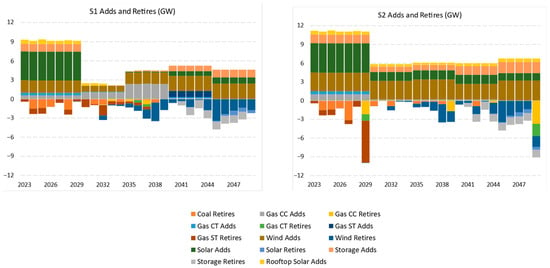
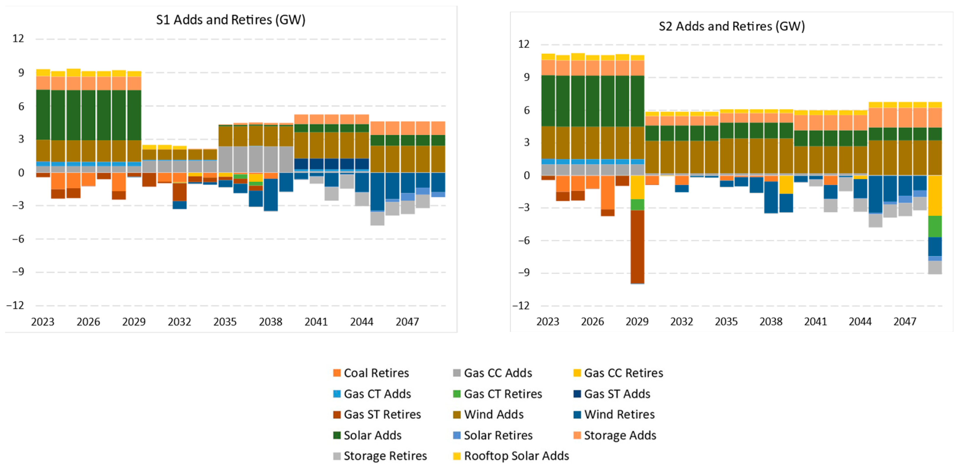
Both mixes in capacity (gigawatts, GW) and share (percentage) of total installed capacity are found in Table 1. Capacity additions and retirements from 2023 through 2049 for S1 and S2 are shown in Figure 1. We do not add or retire any resources in 2050 because we want to have all capacity to be available throughout 2050 when we test the reliability of the system in 2050. Significantly more wind, solar, and BESS and less thermal generation are deployed in S2. Therefore, in S2, we have more CAPEX associated with new wind, solar, and BESS installations, and end-of-life (EOL) abandonment costs associated with thermal plant retirements.

Table 1. Comparison of installed capacities across three scenarios and to 2023 (GW).

Source	2023 (Actual)	S1 in 2050	S2 in 2050
Wind	38 (30%)	63.2 (31%)	92 (40%)
Solar a	17 (13%)	60.2 (29%)	87.7 (38%)
Storage	4.4	11.3	26.2
Gas CC b	35.3 (28%)	54.9 (27%)	37.5 (16%)
Gas Other	17.2 (14%)	16.2 (8%)	6.9 (3%)
Nuclear	5 (4%)	5 (2.5%)	5 (2%)
Coal	13.6 (11%)	4.9 (2.5%)	2.6 (1%)
Total c	126	205	232

^a total includes 7.2 GW (S1) and 14.6 GW (S2) of rooftop solar; ^b combined cycle; ^c excluding storage, which needs to be charged from other resources before it can be discharged.

Figure 1. Capacity additions and retirements between 2023 and 2049 for S1 (left) and S2 (right). We do not add or retire resources in 2050.

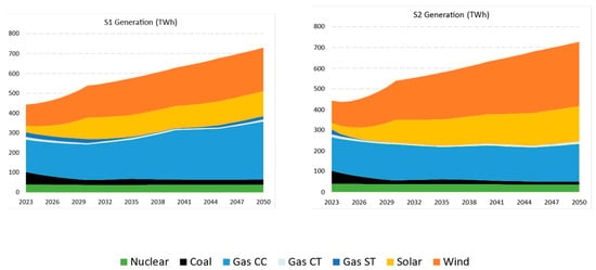
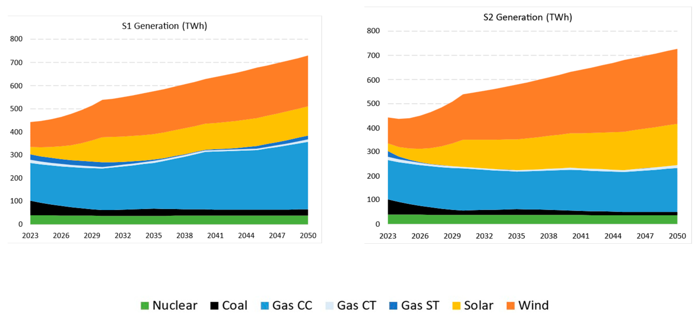
By design, wind and solar power plants are the only resources with increasing generation in S2, replacing thermal generation from coal- and gas-fired plants (Table 2). The share of wind generation, in percent of total 2050 generation, increases from 30 percent in S1 to 43 percent in S2 (relative to 24 percent in 2023), and the share of solar generation increases from 17 percent to 23 percent (relative to 7 percent in 2023). In contrast, the share of generation from combined-cycle gas plants declines from 40 percent to 25 percent. Coal generation in S2 is 50% of S1 generation, as is all other gas generation. Figure 2 shows the generation by resource type between 2023 and 2050 for S1 and S2.

Table 2. Comparison of generation shares across two scenarios and to 2023 (%).

Source	2023 (Actual)	S1 in 2050	S2 in 2050
Wind	24	30	43
Solar	7	17	23
Gas CC	37	40	25
Gas Other	8	4	2
Nuclear	9	5	5
Coal	14	4	2

Figure 2. Generation in TWh by resource type for S1 (left) and S2 (right).

3.3. Development of Consumer Cost of Electricity

The total costs associated with building, operating, and disposing facilities at EOL were calculated for the 2023–2049 period in each scenario. We do not include 2050 costs in our calculations because they would be missing the costs of building and retiring units. As mentioned previously, we confirmed the reliability of the system in 2050 on the basis of units that would be available throughout 2050. The formulations of cost calculations are detailed in Section S3.

We used the CAPEX, and fixed operating and maintenance (FOM) assumptions from EIA (2023) [22]. The CAPEX assumptions are for the ERCOT region. We used the average variable operating and maintenance (VOM) from the dispatch modeling output. We assumed the following fuel prices in real 2023 dollars: $38/ton of coal and $4/MMBtu of natural gas.

For EOL cost estimates, we used 1.4 (CCGT), 2.8 (coal), 1.7 (wind), 4 (solar) and 7 (BESS) percent of the CAPEX of building a new facility of the same type. Our primary reference for power plant decommissioning costs is Raimi (2017) [23]. EPRI (2017) [24] provides estimates on BESS decommissioning. We are not retiring any nuclear units in our ERCOT scenarios. Adding the EOL costs allows us to capture the impact of differences between operational lives of different generation plants [25]. We then divide the total costs associated with each technology by the total 2023–2049 generation of that technology to obtain total cost associated with generation, in units of $/MWh. We call these initial estimates “cost of electricity” (COE) to distinguish them from the theoretical constructs of Ueckerdt et al. (2013) [14] or Idel (2022) [16], which capture all system integration costs. COEs are directly comparable to generic LCOE estimates but they represent the cost of generation in a real system more accurately.

We also calculated some system integration costs through dispatch modeling. For example, in S2, we needed more transmission capacity and BESS capacity to accommodate much larger capacities of wind and solar power plants, while minimizing the curtailment of their generation as much as possible within the constraints of the software architecture. Still, congestion and demand response (large flexible loads, LFL) increased, which are tracked by the dispatch model. We need to add these system integration costs to our COEs to get closer to the “system LCOE” concept of the literature. Note that we still do not capture all system integration costs. To avoid confusion, we will use the term “consumer cost of electricity” (CCOE) because electricity consumers will pay these costs via charges in their electricity bills.

We also offer two alternative calculations. First, we calculate CCOEs focusing only on the incremental changes from S1 to S2. Specifically, we allocate incremental system costs to incremental generation from wind and solar power plants. This is reasonable because, by design, only wind and solar generation increases from S1 to S2 and, more importantly, all additional transmission, BESS and demand response in S2 were needed to accommodate more wind and solar capacity while keeping the curtailment of their generation and congestion costs as low as S1 levels. Second, in its annual report, the independent market monitor (IMM) provides additional system costs. As a result, we also calculate the CCOEs based on the IMM data.

4. Results

4.1. CCOE Estimates Under the Two ERCOT Scenarios

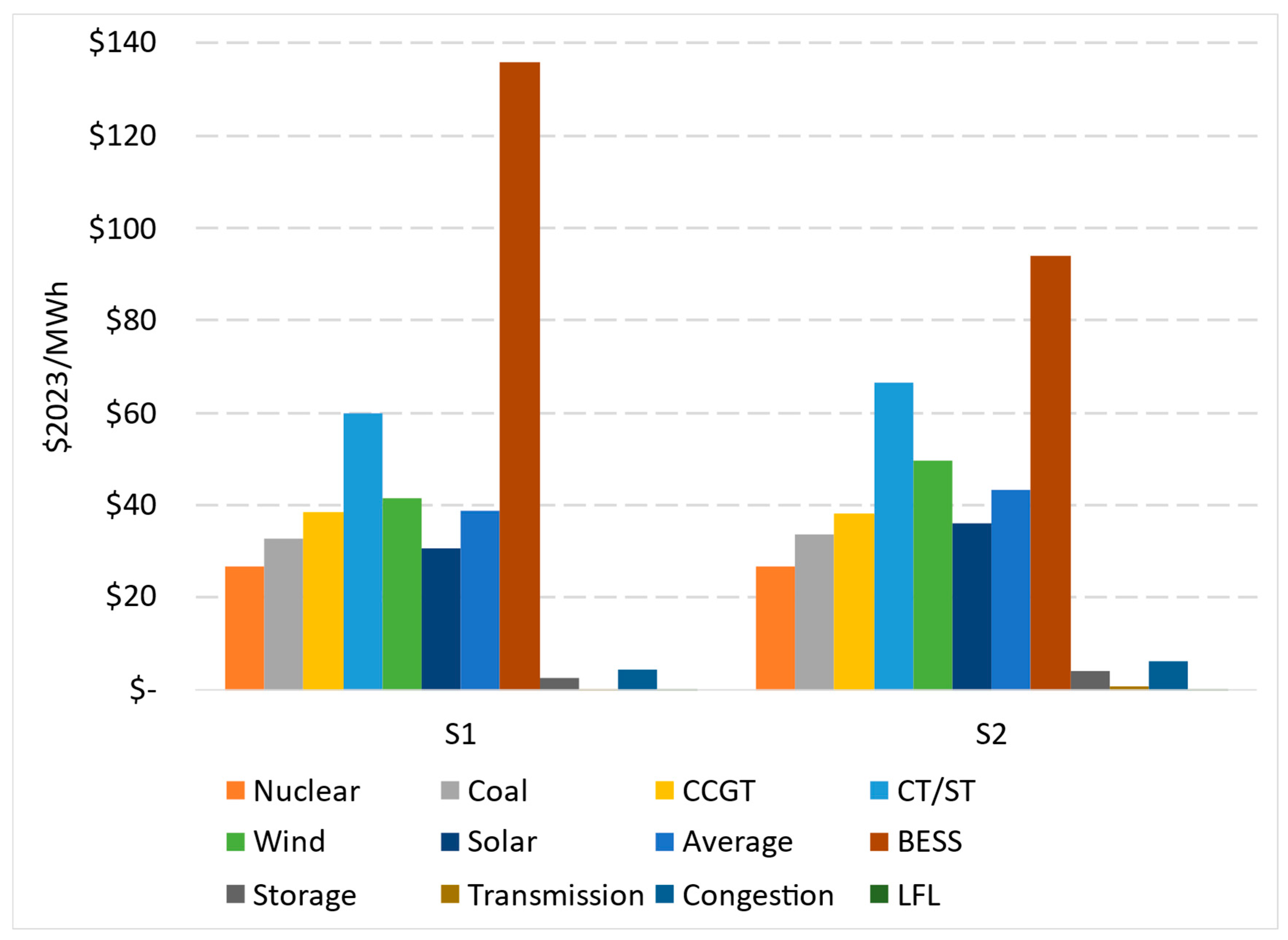
We first compare COEs of each technology to each other; then to the average cost of electricity, calculated by dividing the total cost of building, operating and retiring all generation facilities between 2023 and 2049 by total generation in that period; and, then to per-MWh system costs, which are calculated by allocating costs to total demand (generation) in the system (Figure 3). We offer the following highlights:

• The average cost of electricity in S1 is $38.7/MWh versus $43.4/MWh in S2, representing a 12.1% increase in electricity to the consumer.
• In both S1 and S2, the cheapest source of electricity generation is nuclear (about $27/MWh), followed by solar, coal, CCGT, and wind in S1, and coal, solar, CCGT, and wind in S2. The lower costs of nuclear and coal are because we are not building new nuclear and coal capacities in our scenarios; existing facilities do not incur CAPEX.
• The COE of wind (solar) increases by almost $8/MWh (more than $5/MWh) from S1 to S2. The increases are due to the CAPEX costs of building additional capacity and the lower capacity factors associated with increased curtailment.
• The COE of CT/ST increases by about $6/MWh, which will be discussed later.
• The COE of BESS is high in the ERCOT system for the 2023–2049 period because much of the battery storage capacity that will be available in 2050 will be built over this period, while dispatch from batteries is low.
• When we consider BESS as a system integration cost (rather than as a generator) and allocate total costs to total generation in the system, the incremental storage cost on the system is small (dark gray bar titled “Storage,” with values of $2.5/MWh and $4.2/MWh for S1 and S2, respectively).
• Similarly, per-MWh congestion and LFL costs are small relative to COEs of generation technologies.

Figure 3. COEs for technologies and system integration costs per total generation ($2023/MWh) for two scenarios (S1 and S2) in the ERCOT area, 2023–2049. Average represents total cost of building, operating and retiring all generation facilities between 2023 and 2049 by total system MWh in that period. BESS represents the COE while Storage represents the total cost of building, operating and retiring BESS divided by total system MWh rather than BESS-dispatched MWh. LFL = payments to larger flexible loads providing demand response.

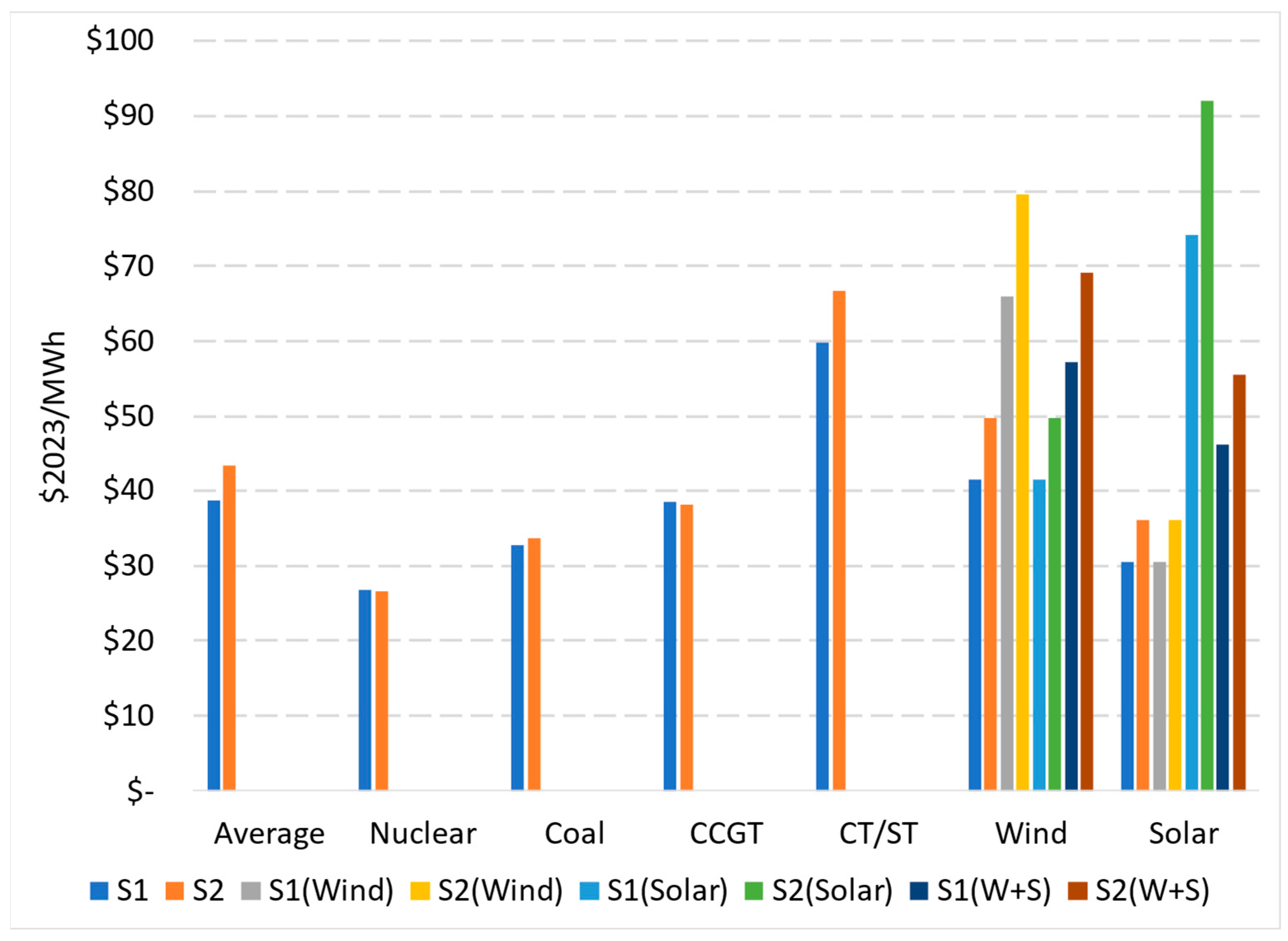
Figure 3. COEs for technologies and system integration costs per total generation ($2023/MWh) for two scenarios (S1 and S2) in the ERCOT area, 2023–2049. Average represents total cost of building, operating and retiring all generation facilities between 2023 and 2049 by total system MWh in that period. BESS represents the COE while Storage represents the total cost of building, operating and retiring BESS divided by total system MWh rather than BESS-dispatched MWh. LFL = payments to larger flexible loads providing demand response.

Next, we follow cost-causation and calculate CCOEs for wind and solar generation by fully allocating all system integration costs to either wind or solar generation. Recall that we add transmission, storage and demand response in the dispatch modeling to reduce curtailment of wind and solar power generation, as well as the congestion caused by the addition of wind and solar capacities in certain regions of the ERCOT system. As such, cost-causation suggests that either wind or solar capacity additions and generation should be fully responsible for related system integration costs. This is not occurring in practice because operators distribute such costs across the system and regulators allocate at least some of the costs (e.g., new transmission costs) across ratepayers. Still, wind and solar CCOEs with full integration costs provide a “maximum” per-MWh value that can be compared to system LCOE estimates from the literature. As an alternative, we assume that wind and solar power generation are “equally” responsible for causing these additional system costs and allocate these costs to the total generation from wind and solar power plants. Current market trends in the ERCOT system (e.g., see ERCOT, 2025 [3]) suggest that solar power plants will be mostly, though not exclusively, responsible for these system integration costs over the next decade. As such, this alternative calculation should be viewed as a “minimum” CCOE for generation from solar power plants.

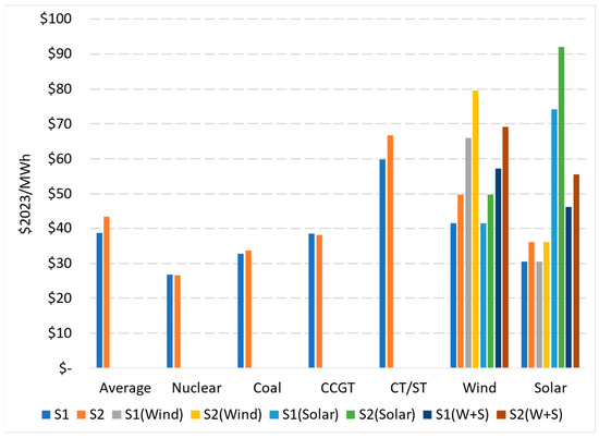
In Figure 4, S1 and S2 costs for each technology are the COEs from Figure 3. The average cost is also shown as a reference to gauge relative contribution of technologies. When we allocate 100% of system integration costs to wind (S1 (Wind) and S2 (Wind)), the CCOE of wind is 59 percent larger in S1 and 60 percent larger in S2 than its COE. When we allocate system integration costs fully to solar power generation (S1 (Solar) and S2 (Solar)), the CCOE of solar generation is also larger than its COE: 142 percent in S1 and 154 percent in S2. Note that cost increases are larger for solar power because solar generation in both scenarios is less than wind generation (Table 2). When we distribute system integration costs across the total generation from wind and solar power plants (S1 (W + S) and S2 (W + S)), CCOEs are smaller but still higher than COEs: 38 and 39 percent for wind, and 51 and 54 percent for solar power generation in S1 and S2, respectively.

Figure 4. CCOEs for wind and solar compared to COEs of all technologies ($2023/MWh); ERCOT, two scenarios, 2023–2049. Three different CCOE estimates are provided: total system costs allocated to wind generation only (Wind), total system costs allocated to solar generation only (Solar), and total system costs allocated to total wind and solar generation (W + S). See Section S4 for formulas.

The COE of dispatchable simple-cycle (CT or ST) gas-fired generators increases nearly $7/MWh in S2 relative to S1. This increase is the net impact of declining CAPEX and increasing OPEX and is caused by the additional wind, solar and BESS capacity in S2, which results in lower generation from gas-fired simple-cycle units that still incur much of the same annual operating costs, especially FOM. Our results show that the grid still needs some CT capacity to provide resource adequacy when wind and/or solar generation fall quickly, and either BESS is not sufficient or transmission bottlenecks necessitate gas-fired units to run at certain nodes of the grid. As a result, the existing CT units must be compensated sufficiently to stay operational while generating less electricity annually. This cost can be seen as a combination of two elements of system integration costs in Ueckerdt et al.’s work (2013) [14]: adequacy cost and full-load hour reduction cost. Our dispatch model results show higher hub prices across the eight ERCOT load zones in four of the five periods that we simulated. These differences range from about $5/MWh to $55/MWh across different zones. The differences are in single digits in 2030 and, only in 2035, prices are $5–10/MWh lower in S2 than S1. These results show that the timing of our wind and solar additions allows the system to benefit from the low dispatch cost of wind and solar power generation in 2035 before further additions, retirement of dispatchable units and load growth (especially in eastern zones of ERCOT where less wind and solar power plants are built) constrain their dispatch and prices eventually become significantly larger in S2 than S1 as time progresses toward 2050.

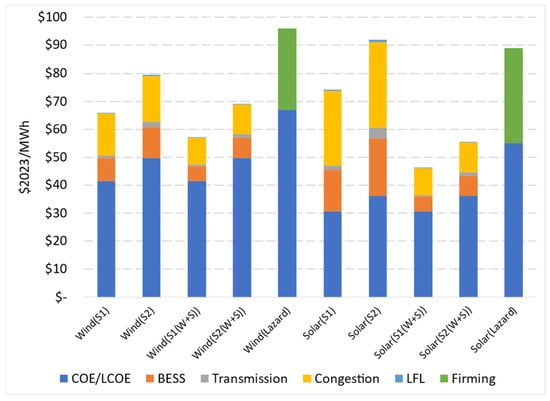
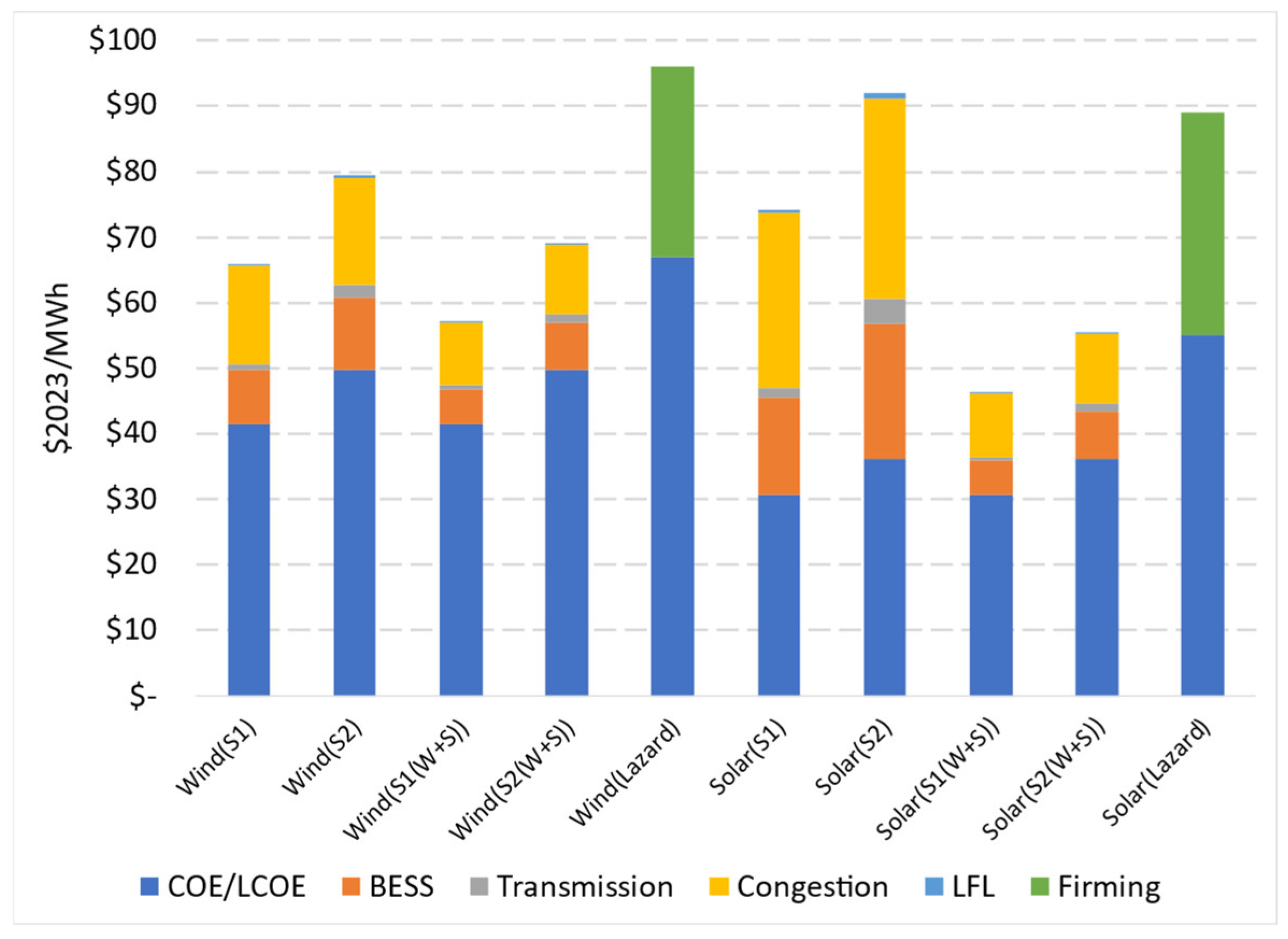
The comparison of our COE and CCOE estimates to unsubsidized LCOEs from Lazard (2025) [17] is informative. Our COE for wind, before system integration costs, is $40/MWh in S1 and $48/MWh in S2, both much lower than the LCOE of $67/MWh in Lazard (2025) [17] (dark blue segments in Figure 5). These differences can be attributed to the inclusion of existing facilities in our simulations, representing a large percentage of operating wind facilities in the ERCOT system, allowing us to waive CAPEX of these facilities. In contrast, generic LCOEs are calculated for a new-build individual power plant. Similarly, our COE for solar power generation is $30/MWh in S1 and $35/MWh in S2, also lower than $55/MWh in Lazard (2025) [17]. Again, although more solar capacity will be built in ERCOT during our study period, when these costs are spread over the 2023–2049 generation from both existing and new facilities, per-unit cost declines.

Figure 5. Breakdown of CCOEs ($2023/MWh) of wind and solar generation. The dark blue segments represent the COEs calculated for our scenarios or LCOE estimates from Lazard (2025) [17].

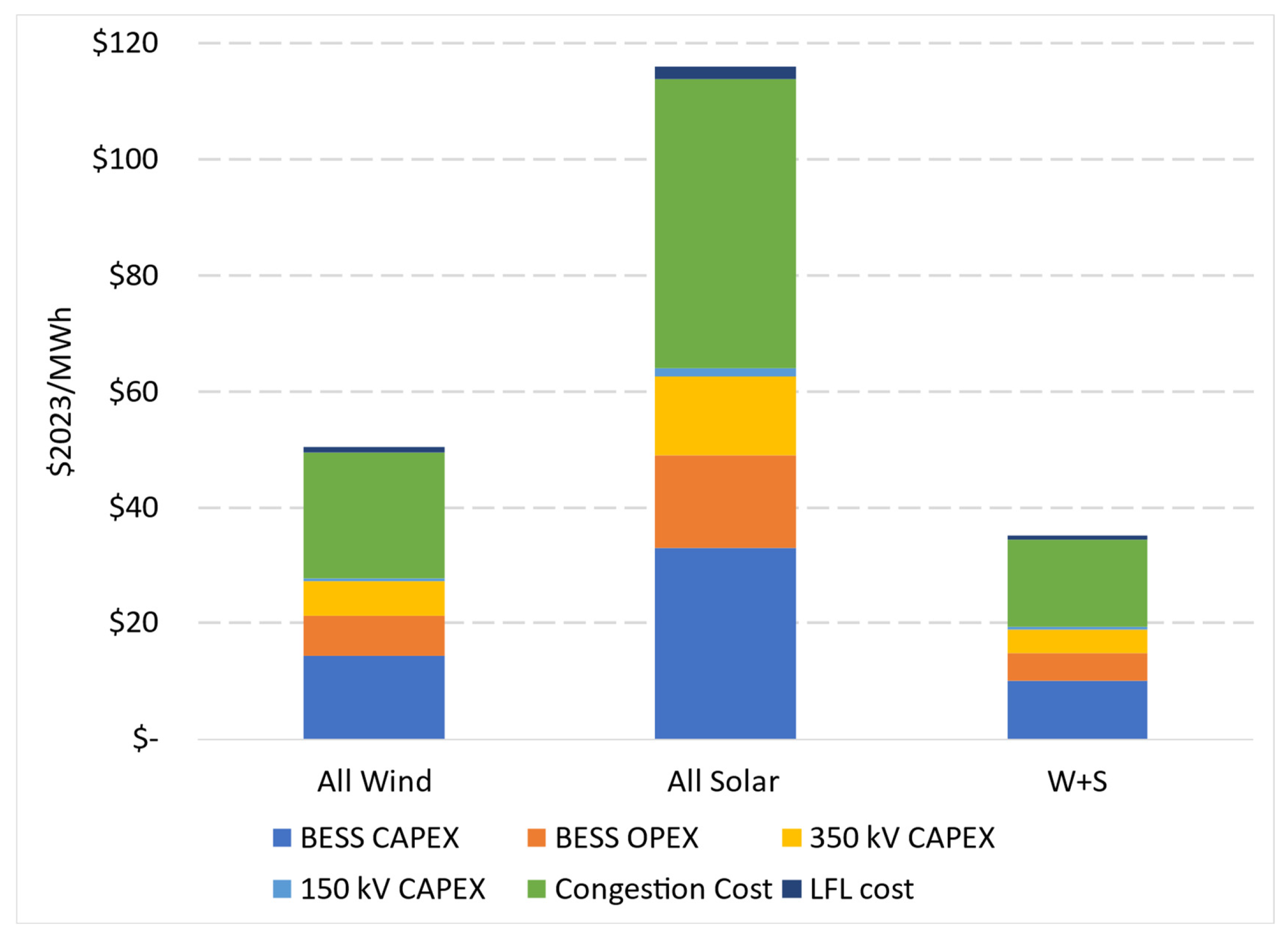
Next, we compare our system integration costs against Lazard’s (2025) [17] firming costs, which represent the cost of backing up an individual wind or solar facility (Figure 5). System costs in wind CCOE are $24/MWh (in S1) and $30/MWh (in S2) as compared to the firming cost of $29/MWh in Lazard (2025) [17]. System costs of solar CCOE range from $43/MWh (S1) to $56/MWh (S2) as compared to the firming cost of $34/MWh in Lazard (2025) [17]. The differences in and higher values for solar power between our analysis and Lazard’s are due to different definitions of system integration costs. Our system integration costs include investment in new transmission and BESS, congestion costs, and payments to LFL, providing demand response. In contrast, Lazard (2025) [17] only considers the cost of backup capacity. As such, it is unsurprising that our system integration cost estimates for wind power are more in line with firming cost estimates for wind by Lazard (2025) [17], as compared to corresponding numbers for solar power. Because most wind capacity is already built, transmission capacity from wind locations in west Texas to load centers in the Dallas–San Antonio–Houston triangle already have been expanded several times (albeit still insufficiently). Perhaps most importantly, wind generation in ERCOT leads to less congestion and requires less backup than solar generation, which peaks during high load hours and declines rapidly in late afternoon to early evening hours when load is still high, especially during summer months. Also, most solar capacity in our scenarios will be built between 2023 and 2049 and will require new transmission in addition to backup generation and storage.

4.2. Alternative Calculation: Incremental Costs from S1 to S2

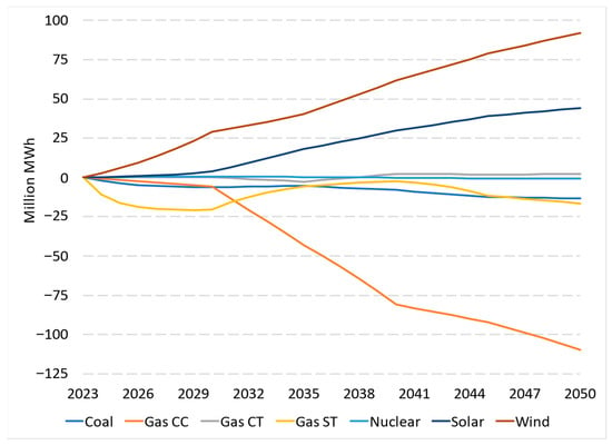
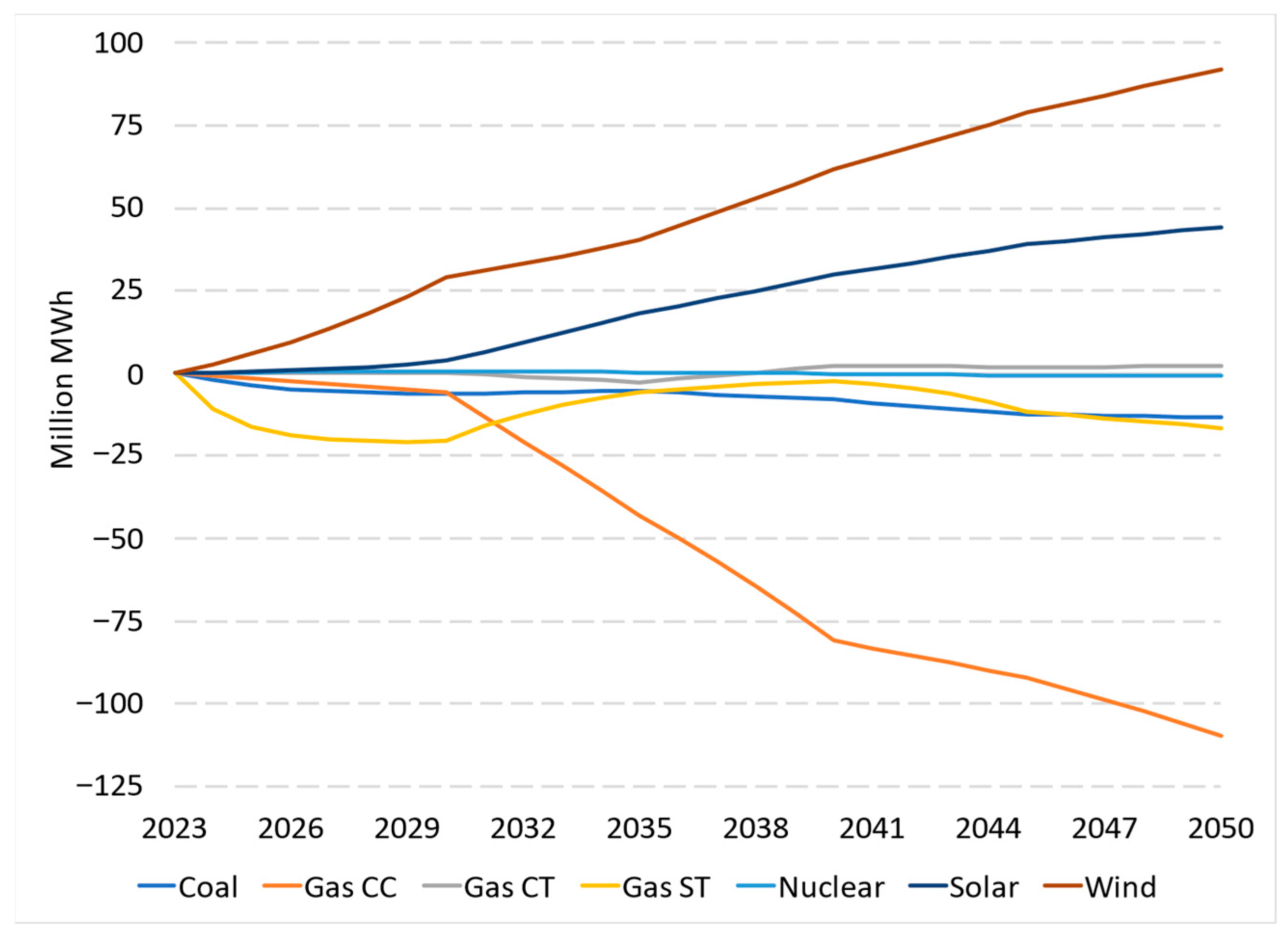
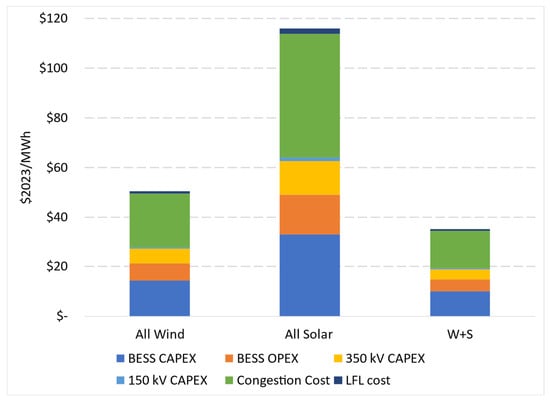
We designed S1 and S2 such that only wind and solar generation (supported by increased transmission and BESS) increase in S2 (Figure 6), while generation from thermal facilities, especially CCGT and coal-fired, decline. If we allocate incremental increases in system integration costs to the incremental increases in generation (Figure 7), per-MWh system integration costs of wind and solar power are higher than our separate calculations for S1 and S2. For wind, incremental system integration costs are about $50/MWh as compared to $24/MWh in S1 and $30/MWh in S2 (Figure 5). For solar power, incremental system integration costs are about $116/MWh as compared to $43/MWh in S1 and $56/MWh in S2 (Figure 5). This result is intuitive. In our previous calculations, all technologies in each scenario benefit from the existing grid infrastructure. However, as the share of intermittent resources increases, system integration costs tend to increase more to maintain reliability while ensuring that these resources maximize their dispatch. When we distribute system integration costs across the total generation of wind and solar power plants, the cost is reduced to about $35/MWh.

Figure 6. Change in generation in S2 from S1.

Figure 7. Allocation of incremental system integration costs to incremental generation in S2 relative to S1. Cost formulations are provided in Section S4.

4.3. Alternative Calculation: Actual ERCOT Costs

The dispatch model implicitly accounts for other system costs identified by Ueckerdt et al. (2013) [14], including costs of curtailment of wind and solar generation, balancing costs, and full-load-hour reduction costs. There is no straightforward way to isolate these costs in the model outputs. Therefore, we do not include these additional system costs in CCOE estimates, although they do show up in higher energy prices in model runs. The average prices across the eight ERCOT load zones and across all five model run years are $6/MWh higher in S2 than in S1. The price increase in S2 relative to S1 is higher in some zones in some of the test years and tends to increase from 2030 to 2050. For example, eight load zone average price increase is nearly $18/MWh in 2050, with a maximum of $27/MWh in the Houston load zone and the minimum of $11/MWh in the South load zone.

However, some of these additional system costs are captured in industry reports. For example, the annual reports of the independent market monitor (IMM) provide some estimates. The “energy cost” item in Table A1 of the 2024 annual report, Potomac Economics (2024) [26] (here, Table 3), represents the cost of electricity purchased at the wholesale market and is akin to average prices discussed in the previous paragraph. The energy cost reflects some system integration costs, such as the need to dispatch more expensive units in times of transmission congestion, but it is still not the total system cost of electricity, which is reported as $35 billion (bottom of Table 3; individual line items are listed in the table). Overall, these additional costs add about $6 billion, or 21 percent of energy costs of $29 billion in 2023.

Table 3. Annual aggregate costs of various ERCOT charges and payments in 2023 [26].

Cost Type	Annual Total ($M)
Energy	28,965
Regulation Up	119
Regulation Down	48
Responsive Reserve	407
Non-Spin	426
ECRS	669
CRR Auction Distribution	(1442)
Balancing Account Surplus	261
CRR DAM Payment	1807
PTP DAM Charge	1613
PTP RT Payment	1836
Emergency Response Service	39
Revenue Neutrality Uplift	109
AS Imbalance Uplift	(7)
ERCOT Fee	247
ERCOT Passthrough Fee	25
Firm Fuel Supply Service	34
Other Load Allocation	5
Net Cost of Electricity	35,161

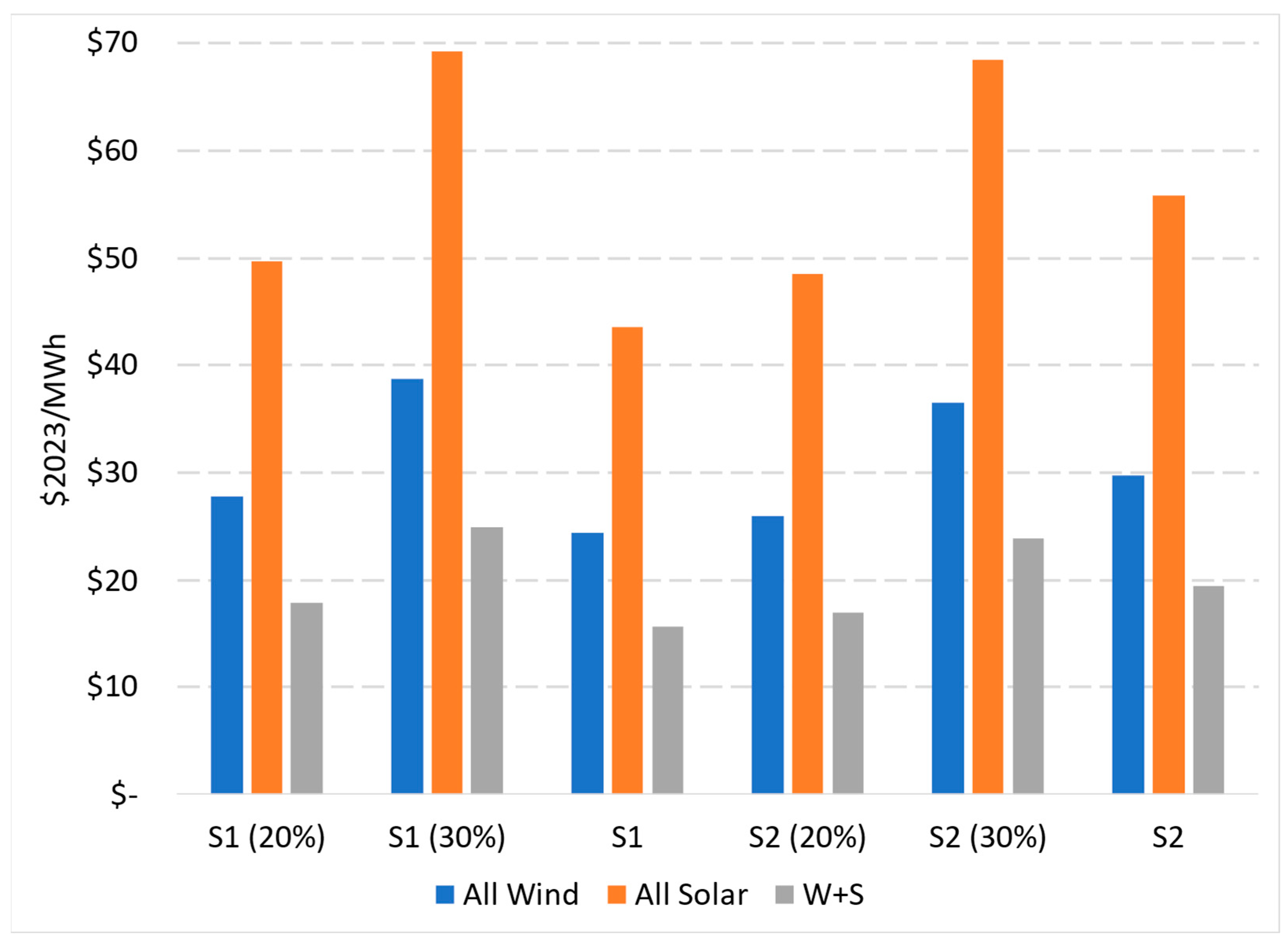
These costs may go higher or lower depending on changes to generation mixes, location of new generation assets versus the evolution of load across different zones, ability to add new transmission capacity, the emergence of demand-side technologies, and many more policy and technology dynamics. In recent years, these additional costs accounted for about 28 percent of total energy costs ($35 billion). In 2022, for example, energy cost was $32 billion and additional costs were $9 billion, or 28% of energy costs from Potomac Economics (2022) [27]. In 2021, energy cost was $66 billion and additional costs were nearly $19 billion, or 28 percent of energy costs from Potomac Economics (2021) [28]. Note that energy cost in 2021 was significantly larger than those in 2022 and 2023 due to the impacts of Winter Storm Uri. Data from our dispatch modeling are not available to calculate additional system costs as in Table A1 of Potomac Economics (2024) [26]. Still, we may add about 20–30 percent of energy costs in our scenarios (Table 4) to reflect potential system balancing costs, keeping in mind that these costs will most likely differ across the scenarios. We calculate system costs at 20 percent of these energy costs, represented as S1 (20%) and S2 (20%) in Figure 8, and 30 percent of these energy costs, represented as S1 (30%) and S2 (30%) (also in Figure 8). In each case, we use the average of 6 years of system costs (Table 4). Then, we allocate the total to 2023–2049 generation of wind only, solar only, or wind and solar together, and estimate an average per-MWh system integration cost. These alternative estimates are higher than our original estimates (Figure 5), because they include more system costs. For example, when all costs are allocated to wind, S1 (20%) system costs are $3/MWh higher than S1, and S1 (30%) costs are $16/MWh higher (blue bars in Figure 8). The only exception is S2 (20%) costs: wind system costs are about $4/MWh lower in S2 (20%) than in S2, and solar system costs are about $9/MWh lower (orange bars in Figure 8).

Table 4. Total Cost of Electricity based on Load Zone Prices from AURORA and 2023 from Potomac Economics (2024) [26] ($2023 billion).

Scenario	2023	2030	2035	2040	2045	2050
S1	$29	$16	$21	$21	$25	$30
S2	$29	$17	$19	$29	$28	$45

Figure 8. Comparing system costs from different calculations. S1 and S2 represent system costs from our calculations (Section S4). S1 (20%) and S2 (20%) are system costs in the two scenarios calculated as 20% of energy costs in the two scenarios (per Table 4) and represent the lower bound of system costs from IMM reports. S1 (30%) and S2 (30%) are system costs calculated as 30% of energy (per Table 4) and represent the upper bound of system costs from IMM reports.

Costs of ERCOT services (Table 3) should cover most of the costs of congestion and demand response from our modeling, but they are silent on the costs of transmission expansion, which we included. Also, we assign the BESS costs directly to wind and/or solar power generation. In contrast, the IMM report [26] captures BESS costs only to the extent they provide some of the services listed in Table 3; they do not include the BESS CAPEX. Moreover, not all ERCOT system costs in Table 3 are caused by the addition of more wind and solar capacity. Nevertheless, these calculations help us appreciate that a system cost calculation more inclusive than ours will likely lead to higher system integration costs. And, if only wind and solar generation is increasing (with BESS backup) over a period of growing system costs (as we experienced when we transitioned from S1 to S2), it is reasonable to deduce that wind and solar additions are the primary cause of these additional costs.

In reality, of course, a power system undergoes multiple changes through a period of 28 years. A more accurate understanding of system costs and the value of different generation technologies (in fact, of individual assets) will require additional granular dispatch modeling that ensures system reliability and availability of electricity to all consumers at all hours.

5. Discussion and Conclusions

The literature on cost of electricity confirms the need for sophisticated modeling of complex electricity systems to produce realistic, system-specific cost estimates. Industry players use a handful of commercial software to ensure reliable system operations, to make investment decisions or to conduct other short- or long-term studies such as transmission planning. But the peer-reviewed literature is lacking studies leveraging these industry-standard software packages that are used for making multi-billion-dollar decisions. We use one of these models, AURORA, to confirm that generation mixes of our two scenarios can meet demands at all times, at all nodes of the ERCOT system, and at the least cost over the study period through 2050. In addition to these standard power system operations criteria, we also minimize congestion costs across the transmission grid and curtailment of wind and solar generation, aiming to achieve same levels across both scenarios. Otherwise, we would not be comparing similarly reliable systems.

We then calculate the cost of electricity (COE), system integration costs, and consumer cost of electricity (CCOE), which is the sum of the first two cost items. Our costs include CAPEX associated with building and retiring power plants, OPEX of generating electricity, congestion costs, cost of building new high-voltage transmission, and some demand response. We also provide two alternative calculations. The first focuses on the allocation of incremental system costs between S1 and S2 to incremental generation of wind and solar power plants—only technologies with increased generation from S1 to S2. The second leverages more itemized reporting of actual costs by the IMM. Overall, these alternative calculations provide reasonable ranges for CCOEs that are consistent with our original estimates.

We offer the following key observations:

• Our ERCOT COE estimates for wind and solar power generation are lower than generic LCOE estimates [17], because, by definition, generic LCOEs calculate the cost of constructing and operating a new power plant regardless of system characteristics. In contrast, we look at the cost of operating existing plants, in addition to building and operating new plants, over a fixed time period. Existing plants meet most of the electricity demand, especially in the early years of our period of analysis. As such, the average cost of electricity from any type of power plant reflects the value of existing plants in the system.
• Variable Energy Resources (VER) technologies bear system integration costs that are larger than those associated with dispatchable resources. These system costs are reflected in the cost of electricity to consumers.

  a.

  In S1, system integration costs are about $24/MWh if all costs are allocated to wind generation, $44/MWh if all are allocated to solar generation, and $16/MWh if allocated to total wind and solar generation.

  b.

  In S2, system integration costs are about $30/MWh if all costs are allocated to wind generation, $56/MWh if all are allocated to solar generation, and $19/MWh if allocated to total wind and solar generation.

  c.

  We designed S2 with more wind, solar, and BESS capacity and less thermal capacity than S1, with only the generation from wind and solar power plants increasing in S2 relative to S1. The incremental system integration costs are $50/MWh if allocated solely to wind generation, $116/MWh if allocated solely to solar generation, and $35/MWh if costs are distributed across total wind and solar generation.

• System integration costs are higher for solar than wind generation because more solar capacity is built during the study period, along with most of the BESS capacity needed to back up primarily solar power plants’ intermittency and variability. Also, solar generation will still be less than wind generation (because of lower CFs and capacity). With larger CAPEX and lower generation than wind power, system integration costs per MWh are larger for solar than wind power.
• Our system integration cost estimates are consistent with the firming costs of Lazard (2025) [17]: $29/MWh for wind and $34/MWh for solar power. Our system integration costs and CCOEs are also aligned with the ERCOT market data as reported by the IMM.
• Comparing S1 COEs (i.e., no system integration costs), nuclear, at $27/MWh, is the lowest cost generation in ERCOT during the study period, followed by solar ($31/MWh), coal ($33/MWh), CCGT ($39/MWh), wind ($42/MWh) and simple-cycle gas ($60/MWh). The average cost of electricity is $39/MWh.
• The average cost of electricity for S2 ($43/MWh) is higher than S1 primarily due to additional costs of installing larger wind, solar and BESS capacities. Accordingly, the COEs of wind and solar power generation increase to $50/MWh and $36/MWh, respectively. In contrast, the COEs of thermal technologies stay roughly the same as in S1: $27/MWh (nuclear), $34/MWh (coal), $38/MWh (CCGT) and $67/MWh (simple-cycle gas).
• The competitiveness of wind and solar costs are reduced when we add system integration costs to COEs to calculate CCOEs. As summarized in bullet 2 above, these costs are $16/MWh in S1, $19/MWh in S2 or $35/MWh in incremental terms when they are allocated across total wind and solar generation.
• The method using IMM data yields similar results. The calculations to allocate system costs to individual technologies provide maximum cost estimates for each technology. Such an estimate may inform analyses of systems when either wind or solar power dominate capacity additions and can be reasonably assessed to cause additional system costs. This is rarely the case in real systems. For example, in the ERCOT system, high-quality wind and solar resources induce capacity additions across fairly wide areas and their generations mostly complement each other; and as long as transmission capacity can catch up, allocating system costs to either wind or solar power alone is not realistic but allocating the system costs to total wind and solar generation would be more reasonable.

Finally, CCOEs depend on individual system characteristics. As such, if the ERCOT system evolves differently than in our S1 and S2 assumptions, the CCOEs must be recalculated, highlighting the site- and assumption-specific nature of the modeling. For example, ERCOT (2024) [29] reports scenarios with updated demand forecasts with rapid growth expected from data centers, green hydrogen projects, and other electrification efforts. Also, some ERCOT (2024) [29] scenarios assume more solar and BESS addition by 2035 than in our study, even in S2. This is an inherent risk of long-term scenario analyses: scenarios can become outdated quickly as technologies, market designs, policies, and more, change. Nevertheless, CCOEs are insightful estimates of costs for system planning and policy discussions for a given power system because they are representative of specific system conditions and are based on nodal dispatch modeling to ensure a high level of reliability throughout the assessment period. In fact, CCOEs should encourage stakeholders to pursue scenarios that are most likely to yield more reliable systems at lower costs.

Although our case study was the ERCOT system, we recommend the CCOE approach with a comparison of different resource mix scenarios for other power systems and its periodic update to ensure that electricity demand can be met reliably and at the least cost at all nodes at all times. Each system is unique in various ways and our COE and CCOE estimates cannot be assumed to apply to other systems. For example, in systems where wind and/or solar quality is not as good as in ERCOT, wind and/or solar CCOEs may be higher. Similarly, in systems where natural gas is expensive, COEs of gas-fired plants will most likely be higher. And, clearly, the ability to develop transmission capacity in a timely manner and the willingness of consumers to provide demand response differ across jurisdictions. These are all reasons why more stakeholders are asking for sophisticated modeling of each power system independently. This is the only way to evaluate energy policies in a way that is directly relevant to that system. Importantly, system operators have much more granular data on their systems and conduct routine modeling exercises to assess the future needs of a reliable system under different scenarios. The calculation of CCOE in a consistent manner across scenarios would provide all stakeholders, but especially policymakers, with an intuitive metric on total cost of electricity to consumers.

References

- Moraski, J.; Qvist, M.; Spokas, K. Beyond LCOE: A Systems-Oriented Perspective for Evaluating Electricity Decarbonization Pathways. Available online: https://cdn.catf.us/wp-content/uploads/2025/06/30100806/CATF_BeyondLCOEReport_Proof_09.30.25.pdf (accessed on 14 December 2025).
- North American Electric Reliability Corporation (NERC). 2024 Long-Term Reliability Assessment. Available online: https://www.nerc.com/globalassets/our-work/assessments/2024-ltra_corrected_july_2025.pdf (accessed on 30 November 2025).
- ERCOT (The Electric Reliability Council of Texas). Report on the Capacity, Demand and Reserves (CDR) in the ERCOT Region, 2026–2030. Available online: https://www.ercot.com/files/docs/2025/05/16/CapacityDemandandReservesReport_May2025_Revised.pdf (accessed on 30 November 2025).
- New York ISO. 2025–2034 Comprehensive Reliability Plan. Available online: https://www.nyiso.com/documents/d/guest/2025-2034-comprehensive-reliability-plan (accessed on 3 December 2025).
- PJM. Energy Transition in PJM: Resource Retirements, Replacements & Risks. Available online: https://www.pjm.com/-/media/DotCom/library/reports-notices/special-reports/2023/energy-transition-in-pjm-resource-retirements-replacements-and-risks.ashx (accessed on 30 November 2025).
- MISO. MISO’s Response to the Reliability Imperative. Available online: https://cdn.misoenergy.org/2024%20Reliability%20Imperative%20report%20Feb.%2021%20Final504018.pdf?v=20240221104216 (accessed on 30 November 2025).
- ERCOT (The Electric Reliability Council of Texas). Long-Term West Texas Export Study. Available online: https://www.ercot.com/files/docs/2022/01/14/Long-Term-West-Texas-Export-Study-Report.pdf (accessed on 22 February 2024).
- Larson, E.; Greig, C.; Jenkins, J.; Mayfield, E.; Pascale, A.; Zhang, C.; Drossman, J.; Williams, R.; Pacala, S.; Socolow, R.; et al. Net-Zero America: Potential Pathways, Infrastructure, and Impacts, Final Report Summary; Princeton University: Princeton, NJ, USA, October 2021; Available online: https://netzeroamerica.princeton.edu/img/Princeton%20NZA%20FINAL%20REPORT%20SUMMARY%20(29Oct2021).pdf (accessed on 22 February 2024).
- IEA (International Energy Agency). IEA WIND TCP Task 25—Fact Sheet. Available online: https://iea-wind.org/wp-content/uploads/2025/02/Task25-FactS-Transmission-February2025.pdf (accessed on 14 December 2025).
- FERC (Federal Energy Regulatory Commission). Order No. 1920-Building for the Future Through Electric Regional Transmission Planning and Cost Allocation. Available online: https://www.ferc.gov/media/e1-rm21-17-000 (accessed on 3 December 2025).
- FERC (Federal Energy Regulatory Commission). 2024 Assessment of Demand Response and Advanced Metering. Available online: https://www.ferc.gov/sites/default/files/2024-11/Annual%20Assessment%20of%20Demand%20Response_1119_1400.pdf (accessed on 22 February 2024).
- ERCOT (The Electric Reliability Council of Texas). 2024 Biennial ERCOT Report on the Operating Reserve Demand Curve. Available online: https://www.ercot.com/files/docs/2024/10/31/2024-biennial-ercot-report-on-the-ordc-20241031.pdf (accessed on 22 February 2024).
- Howland, E. PJM’s Capacity Market Proposal Faces Pushback from Market Monitor, Generators. Utilitydive. Available online: https://www.utilitydive.com/news/pjm-capacity-market-off-cap-must-offer-ferc/737144/ (accessed on 14 January 2025).
- Ueckerdt, F.; Hirth, L.; Luderer, G.; Edenhofer, O. System LCOE: What are the costs of variable renewables? Energy 2013, 63, 61–75. [Google Scholar] [CrossRef] [Scilit]
- Heptonstall, P.J.; Gross, R.J.K. A systematic review of the costs and impacts of integrating variable renewables into power grids. Nat. Energy 2020, 6, 72–83. [Google Scholar] [CrossRef] [Scilit]
- Idel, R. Levelized Full System Costs of Electricity. Energy 2022, 259, 124905. [Google Scholar] [CrossRef] [Scilit]
- Lazard, “Levelized Cost of Energy+”. 2025. Available online: https://www.lazard.com/media/5tlbhyla/lazards-lcoeplus-june-2025-_vf.pdf (accessed on 14 December 2025).
- Manzolini, G.; Binotti, M.; Gentile, G.; Picotti, G.; Pilotti, L.; Cholette, M.E. Actual cost of electricity: An economic index to overcome levelized cost of electricity limits. iScience 2024, 27, 109897. [Google Scholar] [CrossRef] [Scilit] [PubMed]
- Veronese, E.; Manzolini, G.; Moser, D. Improving the traditional levelized cost of electricity approach by including the integration costs in the techno-economic evaluation of future photovoltaic plants. Int. J. Energy Res. 2021, 45, 9252–9269. [Google Scholar] [CrossRef] [Scilit]
- Lazard, “Levelized Cost of Energy+.”. 2024. Available online: https://www.lazard.com/media/xemfey0k/lazards-lcoeplus-june-2024-_vf.pdf (accessed on 17 June 2024).
- Long-Term System Assessment for the ERCOT Region. Electric Reliability Council of Texas. Available online: https://www.ercot.com/files/docs/2022/12/22/2022_LTSA_Report.zip (accessed on 16 February 2024).
- Energy Information Administration. Assumptions to the Annual Energy Outlook 2023: Electricity Market Module. Available online: https://www.eia.gov/outlooks/aeo/assumptions/pdf/EMM_Assumptions.pdf (accessed on 17 June 2024).
- Raimi, D. Decommissioning US Power Plants, Resources for the Future. Available online: https://media.rff.org/documents/RFF20Rpt20Decommissioning20Power20Plants.pdf (accessed on 14 February 2025).
- Electric Power Research Institute. Recycling and Disposal of Battery-Based Grid Energy Storage Systems: A Preliminary Investigation. Available online: https://www.epri.com/research/products/000000003002006911 (accessed on 14 February 2025).
- Emblemsvåg, J. Rethinking the ‘Levelized Cost of Energy’: A critical review and evaluation of the concept. Energy Res. Soc. Sci. 2025, 119, 103897. [Google Scholar] [CrossRef] [Scilit]
- Potomac Economics. 2023 State of the Market Report for the ERCOT Electricity Markets. Available online: https://www.potomaceconomics.com/wp-content/uploads/2024/05/2023-State-of-the-Market-Report_Final.pdf (accessed on 17 June 2024).
- Potomac Economics. 2022 State of the Market Report for the ERCOT Electricity Markets. Available online: https://www.potomaceconomics.com/wp-content/uploads/2023/05/2022-State-of-the-Market-Report_Final_060623.pdf (accessed on 17 June 2024).
- Potomac Economics. 2021 State of the Market Report for the ERCOT Electricity Markets. Available online: https://www.potomaceconomics.com/wp-content/uploads/2022/05/2021-State-of-the-Market-Report.pdf (accessed on 17 June 2024).
- ERCOT (The Electric Reliability Council of Texas). 2024 LTSA Update. Available online: https://www.ercot.com/files/docs/2023/05/12/2024_LTSA_update_20230516_v1.0.pdf (accessed on 16 March 2025).
Disclaimer/Publisher’s Note: The statements, opinions and data contained in all publications are solely those of the individual author(s) and contributor(s) and not of MDPI and/or the editor(s). MDPI and/or the editor(s) disclaim responsibility for any injury to people or property resulting from any ideas, methods, instructions or products referred to in the content. |
© 2026 by the authors. Licensee MDPI, Basel, Switzerland. This article is an open access article distributed under the terms and conditions of the Creative Commons Attribution (CC BY) license.