Distribution Network Fault Diagnosis with Noise-Assisted Multivariate Empirical Mode Decomposition and a Modified Multiple Branch Convolutional Neural Network

Abstract

A novel method based on noise-assisted multivariate empirical mode decomposition (NA-MEMD) combined with a modified multiple branch convolutional neural network (MMBCNN) is designed to detect fault events in distribution networks and to classify various faults in a distribution system. Given the presence of noise components in transient voltage signals, a moving time window technique integrated with the NA-MEMD method is employed to process high-frequency sampling and long-term series signals. This method is also utilized to reliably identify noise components in modal components through permutation entropy. On this basis, the Clarke transform is employed to convert transient voltage signals into the d–q axis, and three-phase voltage waveforms are transformed into a ring image. Moreover, an MMBCNN is developed to accurately detect and classify distribution network faults, and a modified pooling function is introduced to improve feature extraction ability and model convergence performance. Finally, the accuracy and effectiveness of the proposed algorithm are estimated and analyzed using measurement and fault simulation data from distribution networks.

1. Introduction

Power systems are related to a country’s economy, social stability, and security; all power system equipment must operate with high efficiency and be protected against accidents. Line faults caused by nonhuman factors can be mitigated by allowing relays to accurately classify phases. In accordance with actual distribution network protection policies, modern distribution systems are required to maintain the operation of sound phases. Tripping only the faulted phases is critical for ensuring system stability. However, traditional phase classification methods are frequently compromised by factors such as system topology, remote-end infeed, fault resistance, and mutual coupling from adjacent parallel lines [1,2]. Moreover, high-impedance faults, an inherent problem in power distribution, cannot be reliably identified using conventional protection mechanisms. Owing to the developments in information technology and the digital society, increasing attention has been directed toward data-driven methods that enhance the stability and security of distribution networks [3].

Current diagnostic methods for distribution network faults can be broadly classified into impedance methods and artificial intelligence algorithms. Impedance-based analysis methods rely on the physical models of the distribution network after a fault occurs and determine fault locations by analyzing the distribution of fault voltages and currents. In [4], the researchers devised a single-end fault-location algorithm by using a distributed parameter model. The proposed algorithm can determine various fault locations in a network with unbalanced loads and various kinds of feeder lines. In [5], an iterative modification method of capacitive current was proposed to reduce the uncertainty of complex equations with synchronous phasor measurement unit data. However, this method cannot determine the locations of asymmetrical faults. In [6], a fault-location technology for low-current grounding faults was introduced. This method uses zero-sequence voltage fitting functions to determine fault points. Impedance-based analysis methods are applicable to both transmission and distribution networks. However, the accuracy of these fault prediction techniques heavily depends on the precision of impedance parameters and is susceptible to variations in power system operating modes, rendering them incapable of handling complex operational conditions.

Data-driven and artificial intelligence algorithms for fault type detection in distribution systems have attracted considerable interest. These methodologies typically involve feature extraction and fault classification, and typical feature extraction methods include the Fourier transform, the S transform [7], wavelet analysis [8], Wigner–Ville distribution [9], and empirical mode decomposition (EMD) [10,11]. In [7], a fast, adaptive S transform approach was designed to improve the time–frequency resolution and computational efficiency of feature extraction of fault disturbances in distribution networks. In [8], a discrete wavelet transform algorithm adopting zero-sequence voltage and current measurements under several conditions was proposed. In [9], a hybrid approach that incorporates the Wigner–Ville distribution was developed to transform the 1D voltage disturbance signal into an image file. Discrete wavelet analysis and the S transform can provide multiscale signal features and are considered extensions of the Fourier transform. However, the performance of discrete wavelet analysis and the S-transform is constrained by challenges related to mother wavelet selection and computational efficiency. By contrast, EMD is based on the local characteristic time scales of signals and can decompose complicated signals into a series of intrinsic mode functions (IMFs). Moreover, EMD does not require predefined wavelet basis functions and can mitigate the energy leakage problem. Furthermore, EMD is a self-adaptive signal processing method that can handle various complicated signals. In [10], an advanced detection method based on EMD was used to extract the vibration signal features of a high-voltage circuit breaker. In [11], an intelligent approach that applies EMD on the residual current signal was developed to detect high-impedance faults in an active distribution system. In [12], EMD was employed to extract instantaneous features in three-phase current signals. The first-level residue and decision tree were used to classify faults. However, the traditional EMD method usually entails the mode-mixing problem, which is detrimental to the extraction of fault features.

Machine learning models have been deployed for fault detection and classification in transmission lines. Typical methods include support vector machines, decision trees, random forests, and ensemble techniques [13,14,15]. Although these approaches yield decent results, they are prone to overfitting and become computationally intractable when processing a large number of features. With advancements in data storage and transmission technologies, traditional machine learning methods often fail to deliver satisfactory performance on large, noisy datasets.

As for the distribution network detection and classification, deep learning–based models (e.g., convolutional neural network [CNN] models) and recurrent neural networks (long short-term memory networks) have been employed to improve performance [16,17,18,19,20,21,22,23,24]. In [2], an improved stacked sparse denoising autoencoder combined with supervised backpropagation training was proposed as a robust classifier of distribution network faults. Moreover, a power quality detection algorithm based on maximal overlap discrete wavelet transform was applied to determine the initiation and recovery of faults. In [18], a novel CNN-based method for fault identification was proposed, in which fault time–frequency matrices are converted into pixel matrices and used as inputs of CNNs. In [19], a novel hybrid method using a CNN was proposed for fault location and identification in power systems. The Hilbert–Huang transform was adopted to extract fault features. In [20], a CNN model was introduced to classify all kinds of faults in a distribution network integrated with distributed generators. In [22], a new multiscale CNN architecture was proposed to perform multiscale feature extraction and classification for identifying the health conditions of a wind turbine gearbox. In [23], a novel detection method that combines a 1D CNN and a long short-term memory network was proposed for time-series signal pattern recognition and DC–DC converter fault diagnosis. In [24], a novel approach based on an improved 1D CNN was introduced to detect arc faults in distribution networks. However, conventional CNN and 1D CNN models are restricted to extracting spatial features and temporal information, respectively. Moreover, traditional CNN architectures are prone to the gradient explosion issue.

To date, power systems are equipped with a large number of monitoring and protection devices. However, two problems are often encountered during actual data measurement. First, raw data contain a large amount of redundant and noisy data. Second, the sampling rate of recorded fault data is extremely high and requires a large storage capacity. Main features need to be extracted, and noise components must be deleted initially. Moreover, identifying fault characteristics is difficult because of the frequent occurrence of high-resistance grounding fault events. Hence, fault features must be obtained, and advanced technologies must be used to establish fault detection and classification models.

This study proposes a robust multistage fault diagnosis framework based on a modified multiple branch convolutional neural network (MMBCNN) to address the aforementioned problems. In the feature fusion stage, noise-assisted multivariate empirical mode decomposition (NA-MEMD) and permutation entropy (PE) are employed to identify and eliminate noise components within multi-channel data. In the fault classification stage, to standardize data dimensions and mitigate the influence of sampling frequency and data length on the diagnostic model, the Clarke transform is utilized to convert time-series data into 2D images. An MMBCNN-based fault diagnosis framework is proposed to enable online fault detection and classification.

The main contributions of this study are as follows:

(1)

This study presents a novel multistage fault diagnosis framework based on an MMBCNN. The proposed framework encompasses fault data processing, fault detection, and fault diagnosis models. Utilizing the feature extraction and pattern recognition capabilities of the MMBCNN facilitates accurate analysis of the cause of faults. The modeling process of the designed fault diagnosis framework is illustrated in detail.

(2)

A moving time window technique combined with the NA-MEMD is employed to handle multiple high-frequency sampling signals and long-term series signals. It is also utilized to reliably identify noise components in modal components through PE. The adaptive parameter is introduced for the selection of modal components with different degrees of randomness. Moreover, the NA-MEMD method is improved using noise addition and a multidirectional projection mechanism to solve the modal aliasing problem and obtain fault disturbance components accurately.

(3)

A modified pooling function is proposed to improve the model’s convergence performance. In addition, a lightweight CNN is developed by adding a parallel branch, which consists of a 1D CNN and a fully connected network that enables the model to filter input data and extract key fault features. The model mitigates gradient vanishing problems.

This paper is organized as follows. Section 2 introduces the theory of the NA-MEMD and MMBCNN models. The application of the fault waveform reconstruction, feature extraction, and fault detection and classification methods is illustrated in Section 3. Real measurement and simulation data are tested in Section 4. Section 5 concludes the characteristics of the proposed methods and the results of case studies.

2. Basic Methodology

The proposed three-stage methodology for fault diagnosis in distribution networks is illustrated as follows. The first stage identifies the noise components within the distribution network fault waveform. At this stage, NA-MEMD and the PE method are employed. Compared to standard EMD, NA-MEMD incorporates a noise-assisted and multi-directional projection mechanism to effectively resolve the mode mixing problem and accurately extract fault disturbance components. In the second stage, to standardize data dimensions and avoid the influence of sampling frequency and data length on the diagnostic model, the Clarke transform is used to convert transient voltage signals into the d–q axis, which can also comprehensively reflect three-phase fault characteristics. The third stage performs fault detection and classification using the MMBCNN model, where images generated from the fault waveforms serve as input to the proposed fault detector and classifier. The following sections detail the underlying methodologies.

2.1. NA-MEMD

2.1.1. Hammersley Sequence Sampling Method

To explain the Hammersley sequence sampling method, we introduce the relevant concepts of hyperspheres. With regard to the n-dimensional sphere Sⁿ, the radius is o, the vector is s^d, and the definition is illustrated as follows:

$$S^n=\left\{{\mathit{s}}^d\in {\mathit{R}}^{n+1}:‖{\mathit{s}}^d‖=o\right\}$$

(1)

Therefore, the set of directional vectors in n + 1 dimensional space can be equivalent to the set of points on an n dimensional sphere, and Hammersley sequence sampling can achieve uniform sampling in the n + 1 dimensional space.

Hammersley sequence sampling, which is a type of Monte Carlo algorithm [25], utilizes low-difference Hammersley sequences to generate a uniformly distributed set of points on a hypersphere. Compared with uniform angle sampling methods, Hammersley sequence sampling produces a more even sampling point set on a hypersphere. Therefore, this method can provide suitable directional vectors and improve the accuracy of signal average estimation. Details about the Hammersley sequence sampling are presented below.

Step 1: Select a set of prime numbers λ₁, λ₂,…, λ_n, and 2 = λ₁ < λ₂ <…< λ_n.

Step 2: Use the prime numbers to obtain the jth element of the Halton sequence.

$$H_j^z={\displaystyle \frac{g_0}{\lambda }}+{\displaystyle \frac{g_1}{{\lambda }^2}}+{\displaystyle \frac{g_2}{{\lambda }^3}}+\dots +{\displaystyle \frac{g_s}{{\lambda }^{s+1}}}$$

(2)

where g_i is the positive integer, which belongs to [0, z − 1].

Step 3: Use the Halton sequence elements $H_j^z$ to obtain the Hammersley sequence and define the n-dimensional directional vectors with Equation (3).

$$D_j{=(j/N,H}_j^{z_1}{,H}_j^{z_2},\dots {,H}_j^{z_{n-1}}) j=0,\dots ,N-1$$

(3)

2.1.2. Waveform Decomposition Method

To prevent mode aliasing, the noise-assisted multivariate EMD is proposed [26], which introduces white noise signals as auxiliary channels and employs Hammersley sequence sampling for multivariate EMD. By decomposing a set of q multivariate channel signals and p Gaussian white noise signals, the IMF components of q + p channel signals can be obtained simultaneously. Compared with an EMD method with added noise, NA-MEMD reduces the interference of noise signals on the original signal and requires lower computational cost. The details about the NA-MEMD method are illustrated as follows.

Step 1: Construct Gaussian white noise signals, each with the same length as the original signal.

Step 2: Combine q multivariate original signals and p white noise signals into q + p channel signals. The q + p channel signals are defined as $\mathit{s}=({\mathit{x}}_1,{\mathit{x}}_2,\dots ,{\mathit{x}}_{q+p}{)}^T$.

Step 3: Generate a uniformly distributed set of points on the q + p − 1 dimensional hypersphere through Hammersley sequence sampling. The jth directional vector is defined as D_j.

Step 4: The q + p channel signals are projected onto the direction sets, and the maximum and minimum values of these channel signals are calculated. The maximum points and minimum points at the jth projection direction are defined as $({\mathit{t}}_{\mathit{max}}^j,{\mathit{s}}_{\mathit{max}}^j)$ and $({\mathit{t}}_{\mathit{min}}^j,{\mathit{s}}_{\mathit{min}}^j)$. Then, the envelope of signals E^j [27] is obtained through cubic spline interpolation. The average envelope of signals M is calculated as follows:

$$\mathit{M}={\displaystyle \frac{1}{L}}{\displaystyle \sum _{j=1}^L{\mathit{E}}^j}$$

(4)

where L is the total number of directions.

Step 5: The rest signals V = s − M, if the multivariate signals satisfy the IMF stop condition, then V is determined as the IMF components. And the signals are updated as s = s − V, which is assessed on the basis of EMD stop conditions. If the IMF stop condition for the multivariate signal is not satisfied, then the residual V is regarded as the signal curve s. Repeat Step 4 until the IMF stop condition is met.

Step 6: The multivariate signal is decomposed into K IMF components.

$$\mathit{s}={\displaystyle \sum _{c=1}^K{\mathit{V}}_c}+\mathit{r}$$

(5)

where V_c is the cth IMF component of the q + p channel signals and r is the residue.

2.2. Permutation Entropy

Signals are analyzed using PE for the identification of the noise signal. This approach is based on the assumption that patterns do not have the same probability of occurrence in a noise signal. The PE facilitates the quantitative evaluation of a signal’s randomness.

A signal is defined as v_k and its embedding vector vⁱ can be obtained as follows:

$${\mathit{v}}^i=\left\{v_k\right\}, k=i,i+l,\dots ,i+(m-1)l,$$

(6)

where l is the time delay and m is the embedding dimension. According to the experimental results, the parameter m should be between 3 and 7 [28], and i is in the range [1, N − (m − 1)l]. Then, the elements in vⁱ are arranged in ascending order.

$${\mathit{v}}^i{=[v}_{{i+(j}_1-1)l}\le v_{{i+(j}_2-1)l}\le \dots \le v_{{i+(j}_m-1)l}],$$

(7)

Given the condition that $v_{{i+(j}_1-1)l}{=v}_{{i+(j}_2-1)l}$, these elements are ordered according to the smaller value of j_k. Therefore, each vⁱ can be represented as G_i = {j_k}, $k=1,2,\dots ,m$.

The probability of each permutation G_i is defined as P_i. Therefore, the PE of the time series {v_k} is defined as follows:

$$E_P=-{\displaystyle \sum _{i=1}^{k_P}{P}_i{\mathit{lnP}}_i},$$

(8)

where E_P is the PE, k_P is the total number of permutation types, and k_P satisfies the condition $k_P\le m!$. If the selected IMF component is not the noise component, then the E_P should satisfy Equation (9).

$$0\le E_P\le {\delta \overline{E}}_P,$$

(9)

where $\delta$ is the adaptive parameter and ${\overline{E}}_P$ is the PE when P_i = 1/k_P, $i=1,2,\dots {,k}_P$. As the adaptive parameter $\delta$ decreases, the randomness of a selected component decreases. Therefore, by changing the adaptive parameter $\delta$, this method can effectively remove noise components. In this study, a grid search optimization is employed to determine the adaptive parameter $\delta$. The search range for $\delta$ is defined as $[C_{\delta }^{\min }$,$C_{\delta }^{\max }]$, with a search step of C_S. The total number of iterations is $(C_{\delta }^{\max }-C_{\delta }^{\min })/C_S$, and the optimization objective is to minimize the deviation between the standard signal and the reconstructed signal. Consequently, the adaptive parameter δ is set to 0.5 in this study.

2.3. Convolutional Neural Network

Widely used in image object detection and image classification tasks, CNNs extract key features through convolutional and pooling layers. One typical CNN architecture modification involves the addition of parallel branches, and another involves the addition of attention modules [29]. The first improves feature extraction performance and prevents gradient vanishing, whereas the second captures the multiscale characteristic of images by highlighting key features. The proposed modified CNN belongs to the first type.

(1) Multiscale feature learning: In this process, high-dimensional features are extracted from an image by using multiple convolutional and pooling layers. For example, in a two-layer CNN, convolutional layers are denoted as CN1 and CN2, and pooling layers are denoted as PL1 and PL2. Therefore, each feature map contains information at different spatial scales.

A fault map of size CI is input to CN1. We move a filter of size CK across the entire input fault map to obtain local features. Feature map output z is defined as follows:

$$\begin{array}{l}{z}_{i,k}=\sigma \left({\displaystyle \sum _{n=i}^{i+\mathit{CK}-1}{\displaystyle \sum _{m=k}^{k+\mathit{CK}-1}{w}_{n-i+1,m-k+1}{u}_{n,m}}}+b\right),\\ \hspace{1em}\hspace{1em}\hspace{1em}\hspace{1em}\hspace{1em}\hspace{1em}i,k=1,2,\dots ,\mathit{CI}-\mathit{CK}+1\end{array}$$

(10)

where z_i,k is the element of the output feature map at (i, k), w_n-i+1,m-k+1 is the element of the convolutional kernel function matrix at (n − i + 1, m − k + 1), u_n,m is the element of the input feature map at (n, m), b denotes the bias term, and $\sigma (\cdot )$ is an activation function. Common activation functions include sigmoid and rectified linear units, which accelerate model convergence [22]. After deriving the first convolutional layer, we obtain the new feature map z, which is expressed as

$${z=\{z}_{i,k}\} i,k=1,2,\dots ,\mathit{CI}-\mathit{CK}+1.$$

(11)

Then, z is pooled for the extraction of key feature information. In this study, an improved pooling layer model with a pool size of CP is adopted. An updated map ($\tilde{\mathit{z}}$) is obtained using Equations (12)–(14).

$$\tilde{\mathit{z}}=\left\{{\tilde{z}}_{i,k}\right\} i,k=1,2,\dots {,N}_z,$$

(12)

$$N_z={\displaystyle \frac{\mathit{CI}-\mathit{CK}+1}{\mathit{CP}}},$$

(13)

$$\begin{gathered} \left\{\begin{array}{c}{\tilde{\mathit{z}}}_{i,k}={\displaystyle \frac{{\overline{\lambda }z}_{i,k}^{\mathit{max}}+(1{-\overline{\lambda })z}_{i,k}^{\mathit{mean}}-z^{\mathit{min}}}{z_{\mathit{max}}{-z}_{\mathit{min}}}}\hfill \\ z_{i,k}^{\mathit{max}}=\underset{(i-1)\mathit{CP}+1\le n\le \mathit{iCP}, \\ (k-1)\mathit{CP}+1\le m\le \mathit{kCP}}{\mathit{max}}\left\{z_{n,m}\right\} \hfill \\ z_{i,k}^{\mathit{mean}}={\displaystyle \frac{1}{{\left(\mathit{CP}\right)}^2}}{\displaystyle \sum _{n=\mathit{iCP}- \\ \mathit{CP}+1}^{\mathit{iCP}}{\displaystyle \sum _{m=\mathit{kCP}- \\ \mathit{CP}+1}^{\mathit{kCP}}{z}_{n,m}}}\hfill \end{array}\right., \end{gathered}$$

(14)

where ${\tilde{z}}_{i,k}$ is the element in the pooled feature map, $\overline{\lambda }$ is the coefficient used to balance $z_{i,k}^{\mathit{max}}$ and $z_{i,k}^{\mathit{mean}}$ within the pooling function, and $z^{\mathit{max}}$ and $z^{\mathit{min}}$ denote the maximum and minimum elements in the current layer feature map z, respectively.

The feature maps are then processed using CN2 and PL2 models. The operations of CN2, which are expressed in Equations (10) and (11), are adopted. We assume that the number of output feature maps from the second convolutional layer is K₂. Therefore, all feature maps can be denoted as follows:

$${\mathit{q}}_s=[{z^{\prime }}_1,{z^{\prime }}_2,\dots ,{z^{\prime }}_{K_2}],$$

(15)

where ${\mathit{q}}_s$ is the feature map of the sth branch. ${z^{\prime }}_{K_2}$ is the element of the feature map. Map ${\mathit{q}}_s$ is used as the input of PL2 to reduce its size. Then, the feature map ${q^{\prime }}_s$ is obtained using Equations (12)–(14). The concatenation of the learned representations of all the processed feature maps is expressed as

$$q=[{q^{\prime }}_1,{q^{\prime }}_2,\dots ,{q^{\prime }}_{n_{\mathit{pb}}}],$$

(16)

where n_pb is the total number of branches.

In the fully connected layer, the softmax function is applied to yield a conditional probability for each class [30]. Equation (17) is used to calculate the output probability $O_l\in [0,1]$, which is used in the classification of the type of distribution network fault.

$$O_l{=e}^{{(\theta }_l\mathit{q})}/{\displaystyle \sum _{l=1}^{n_f}{e}^{{(\theta }_{l}q)}},l=1,2,\dots {,n}_f,$$

(17)

where n_f refers to the classes of distribution network faults, ${\theta }_l$ is the model parameter, and ${\displaystyle {\sum }_{l=1}^{n_f}}{O}_l=1$.

(2) Parallel Block Learning: Traditional CNN models typically consist of multiple convolutional and pooling layers stacked together. However, a CNN model with numerous layers can easily cause gradient vanishing. Based on residual blocks [31], which enhance feature learning ability by setting skip connections, a CNN with a parallel branch is proposed. The parallel branch consists of a 1D CNN and is a fully CNN. Parallel branches facilitate the feature extraction at different scales. Meanwhile, an MMBCNN operates in an end-to-end learning manner. Given the structure of the proposed CNN model, the model is effective in mitigating gradient vanishing. The CNN output of the main branch is presented as Conv(u), and the parallel branch is denoted as Pb(u). The output of the MMBCNN, y, is calculated as follows:

$$y=\mathit{Conv}(u)+\mathit{Pb}(u).$$

(18)

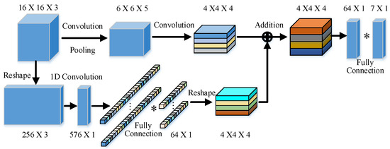
The structure of the proposed MMBCNN-based fault classification model is depicted in Figure 1. The MMBCNN features two branches, with the feature map size and number of channels explicitly annotated at each block. The arrows in the diagram indicate the steps for processing the fault dataset. For the first convolutional layer, $5\times 5$ kernels are designed, while $3\times 3$ kernels are constructed for the second. The pooling size is set to $2\times 2$. Moreover, (*) denotes the fully connected layer in CNN in Figure 1.

Figure 1. Structure of the MMBCNN model with two branches.

As illustrated in Figure 1, the image data processing workflow within the MMBCNN proceeds as follows: In the parallel branch, image data are first converted into feature vectors, upon which a 1D CNN operates to filter features. Subsequently, a fully connected network extracts key feature vectors, which are then transformed back into image data. Finally, the processed data from the backbone network and the parallel branch are summed element-wise.

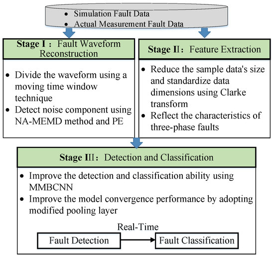
Based on the previous methodologies, the proposed three-stage fault diagnosis framework is illustrated in Figure 2. Stage I reconstructs the fault waveform by mitigating noise components. Stage II performs feature extraction. Finally, Stage III executes fault detection and classification.

Figure 2. Multistage fault detection and classification framework.

3. Application

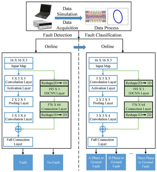
This section mainly uses NA-MEMD and PE to process fault data. The MMBCNN model is employed to detect and classify fault events. The details are shown in Figure 3. The blue lines and green lines indicate main branch and parallel branch.

Figure 3. Flowchart of the fault diagnosis framework based on MMBCNN.

Step 1: Distribution network fault data are obtained using the simulation model, and real measurements are derived with the data acquisition system. The NA-MEMD method is used to split fault waveforms into several components through sifting. Then, a reconstruction method is proposed through PE to delete noise components.

Step 2: The fault disturbance period is detected, and the processed fault waveform is transformed into a 2D image through the Clarke transform. The image data are divided into several groups for training and testing models. Fault detection and classification models based on MMBCNN are established using training samples. Moreover, the online fault detection and classification models are obtained.

Step 3: Real measurements and simulated data are used as test sets to verify the performance of the built model in terms of indicators, such as accuracy and recall.

3.1. Fault Waveform Reconstruction

Fault waveform reconstruction consists of two parts, namely, NA-MEMD and PE. Algorithm A1, which is used to remove the noise component of the fault waveform, is given in the Appendix A. The main steps of fault waveform reconstruction are illustrated as follows.

The raw data are preprocessed using a sliding time window, which partitions the data into multiple segments. NA-MEMD and PE are applied to each segment to accentuate the characteristics of temporal variations. The noise components, i.e., high-frequency terms, and the intrinsic mode functions for each segment are retained. The original fault waveform is subsequently reconstructed by summing the medium- and low-frequency IMFs.

3.2. Feature Extraction

The Clarke transform is applied to reconstructed fault waveforms ${\hat{v}}_{a,t}$, ${\hat{v}}_{b,t}$, and ${\hat{v}}_{c,t}$ for the extraction of fault characteristics. The transformed vectors are denoted as ${\hat{v}}_{\alpha ,t}$, ${\hat{v}}_{\beta ,t}$, and ${\hat{v}}_{0,t}$. The details of the Clarke transform are defined as follows [32]:

$$\left[\begin{array}{c}{\hat{v}}_{\alpha ,t}\\ {\hat{v}}_{\beta ,t}\\ {\hat{v}}_{0,t}\end{array}\right]={\displaystyle \frac{2}{3}}\left[\begin{array}{ccc}1& -1/2& -1/2\\ 0& \sqrt{3}/2& -\sqrt{3}/2\\ 1/2& 1/2& 1/2\end{array}\right]\left[\begin{array}{c}{\hat{v}}_{a,t}\\ {\hat{v}}_{b,t}\\ {\hat{v}}_{c,t}\end{array}\right]$$

(19)

Moreover, the Clarke transform is expressed as Equation (20) under the d–q axis.

$${\mathit{sv}}_t{=\hat{v}}_{\alpha ,t}{+j \hat{v}}_{\beta ,t}={\displaystyle \frac{2}{3}}\left[\begin{array}{ccc}1& e^{j2\pi /3}& e^{j4\pi /3}\end{array}\right]\left[\begin{array}{c}{\hat{v}}_{a,t}\\ {\hat{v}}_{b,t}\\ {\hat{v}}_{c,t}\end{array}\right]$$

(20)

where sv_t is the space vector. The space vector rotates with frequency, which is equal to the system frequency. When the three-phase voltage waveform is symmetrical, the space vector projection on the d–q axis is circular. By contrast, the fault voltage waveform on the d–q axis is elliptical. Therefore, CNN models can be utilized to extract image features and classify fault types. To improve the fault classification accuracy, the fault disturbance period is detected by the maximal overlap discrete wavelet transform method [2].

3.3. Detection and Classification

This study proposes a fault diagnosis model that is based on an MMBCNN to conduct online detection and classification of distribution network faults. Notably, feed line fault detection must be implemented within an extremely short time. Algorithm A2, which shows the details of the training process for MMBCNN, is given in the Appendix A. The main steps of the fault diagnosis model training are shown as follows.

The feeder fault and normal feature sets $(\overline{u},\overline{y})$, are partitioned into several subsets. For fault detector training, a 2-fold cross-validation method is adopted, whereas for fault classifier training, a 10-fold cross-validation approach is used. The weights, biases, and training parameters of the MMBCNN are initialized; specifically, weights are initialized using Xavier’s method, and the Adam optimizer is employed for training. The test set $({\overline{u}}_{\mathit{test}},{\overline{y}}_{\mathit{test}})$ is then input into the MMBCNN model to evaluate the detection accuracy and classification accuracy of detector DP and classifier CP.

The proposed method improves the robustness of the CNN by adding a parallel branch. In practical applications, the fault detector DP always operates online. When a fault is detected, the fault type is classified by CP in an extremely short time.

4. Case Studies

Simulation data based on MATLAB/SIMULINK 2025b and actual data are used to validate the performance of the proposed diagnosis model. The single-, double-, and three-fault, and normal operation comprise the validation dataset. Moreover, all simulations are performed using an Intel Core i7-8850U 2.4 GHz CPU with 16 GB of RAM.

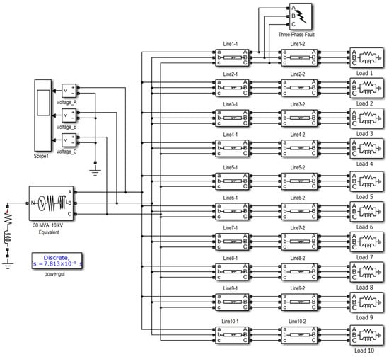
The amount of simulation and actual measurement data for each type of feed line fault is shown in Table 1, where SG_a, SG_b, and SG_c denote single-phase to ground fault; DG_ab, DG_ac, and DG_bc denote double-phase to ground fault; TG indicates three-phase to ground fault; and GP refers to the distribution network’s regular operation. We obtain various simulation data by setting different model parameters. The modifiable parameters include fault location, fault occurrence time, and fault resistance. The configuration details of the fault cases are presented in Table 2, and the structure of the simulation model is depicted in Figure 4. In this figure, the line model consists of one set of resistor-inductor series elements, where port a/b/c connects to the resistor, and port A/B/C connects to the inductor. The simulation model parameters can refer to Reference [33].

Table 1. Number and causes of feed line fault records.

Causes	Distribution Network Faults
Types	SGa	SGb	SGc	DGab	DGac	DGbc	TG	GP
Simulated data	300	300	300	300	300	300	300	600
Real data	150	150	150	150	150	150	150	200

Table 2. Configuration for fault case simulation.

Parameter	Distribution Network Faults
Types	SGa/SGb/SGc/DGab/DGac/DGbc/TG
Fault line	Feeder lines L1–L10
Fault location (km)	0.9, 1.5, 3
Fault inception angle (degrees)	0, 180, 270
Fault resistance (Ω)	5, 100, 1 k, 10 k, 20 k

Figure 4. Simulation of the distribution network.

The data structure of the simulated and actual measurement data is provided in Table 3. The table shows differences in the sampling accuracy of the actual data. The actual sampling frequency range is 128–20,000 samples per cycle due to the various types of monitoring equipment. However, differences in the duration of different types of faults are found. Therefore, the recording time of actual fault events is distributed between 200 and 1000 ms.

Table 3. Data structure.

Data Type	Distribution Network Faults
	Simulated Data	Real Data
Resolution	256 samples per cycle	128–20,000 samples per cycle
Duration	200–800 ms	200–1000 ms

4.1. Analysis of Detection and Classification Methods for Feed Line Faults

This section discusses the different performance metrics, namely, accuracy, recall, precision, and F1-score, on the basis of indicators [20]. The effects of the CNN structure on detection and classification accuracy are analyzed, and the effectiveness of the proposed diagnosis algorithm for feed line faults is assessed.

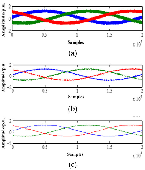
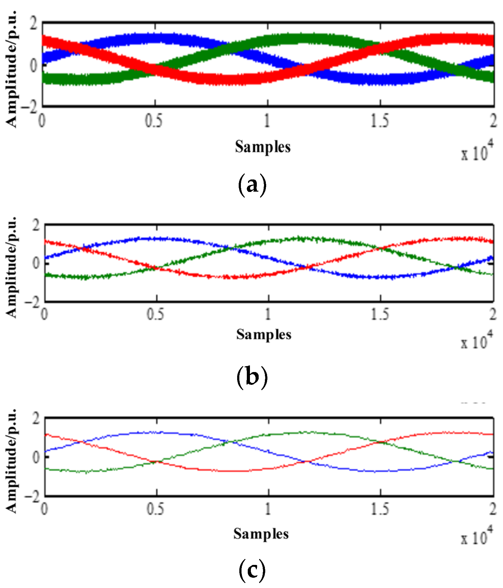
PE is applied to process waveforms with 20,000 samples per cycle to reveal the effectiveness of the proposed waveform reconstruction method in handling high-frequency sampling and long-term series signals. The window size N_t is set at 1000, and the results are illustrated in Figure 5. In this figure, the blue, green and red curves represent a-/b-/c-phase voltage signal. When the adaptive adjustment factor δ decreases, few noise components are included in the reconstructed waveform. The denoising performance is evaluated using the signal-to-noise ratio, defined by Equation (21). The energy ratio, defined by Equation (22), represents the proportion of energy retained in the denoised signal relative to the original signal. Moreover, the standard deviation (SD) of the difference between the standard signal and the denoised signal is also employed to assess denoising performance.

Figure 5. Voltage waveform: (a) original waveform, (b) reconstructed waveform δ = 0.8, and (c) reconstructed waveform δ = 0.5.

Table 4 presents a comparative analysis of the denoising methods. The test signal is the normalized a-phase voltage signal under various noise levels, with a total of N_s = 2560 sampling points. Although wavelet packet decomposition (WPD) removes more signal energy, the NA-MEMD method achieves a lower standard deviation, indicating that the denoised signal more closely approximates the standard signal. Therefore, the NA-MEMD combined with PE outperforms WPD. To ensure the reliability of these results, all experimental outcomes are averaged over 10 independent trials.

$$S_R=10\mathit{log}\left[{\displaystyle \frac{{\displaystyle {\sum }_{i=1}^{N_s}{v}_i^2}}{{\displaystyle {\sum }_{i=1}^{N_s}{{(v}_i{- v \prime }_i)}^2}}}\right]$$

(21)

$$E_{\mathit{SN}}=\left[{\displaystyle \frac{{\displaystyle {\sum }_{i=1}^{N_s}{{( v \prime }_i)}^2}}{{\displaystyle {\sum }_{i=1}^{N_s}{v}_i^2}}}\right]$$

(22)

where $v_i$ and ${ v \prime }_i$ represent the original and denoised time-series data. S_R and E_SN are the signal-to-noise ratio and energy ratio.

Table 4. Comparative analysis of various denoising methods.

Noise Level	50 dB		30 dB
Methods	WPD	NA-MEMD + PE	WPD	NA-MEMD + PE
SR	47	52	30	35
ESN	93.1%	96.2%	82.7%	86.5%
SD	0.0045	0.0031	0.0434	0.0285

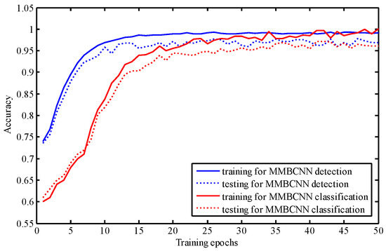
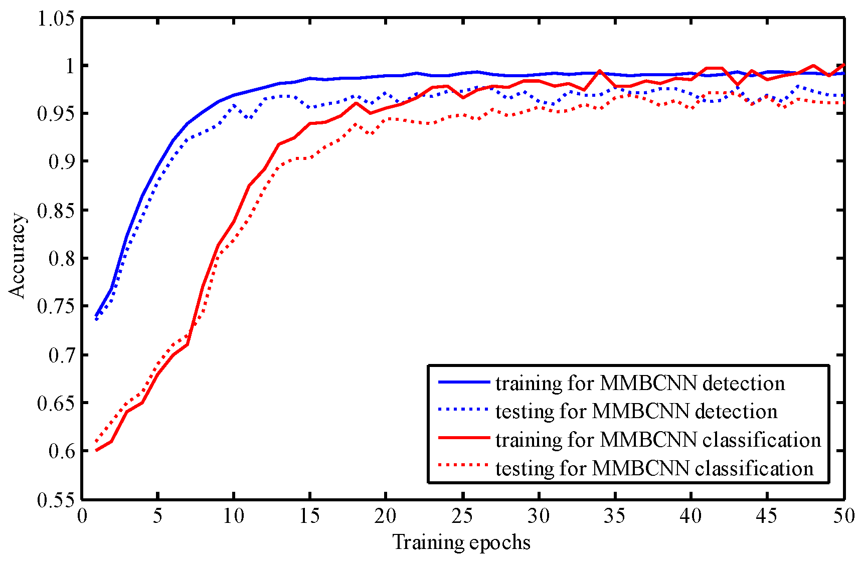
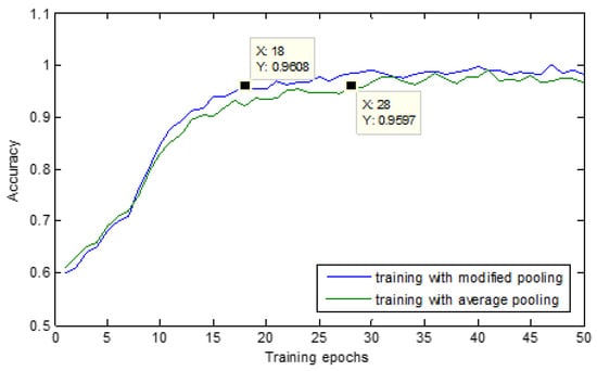
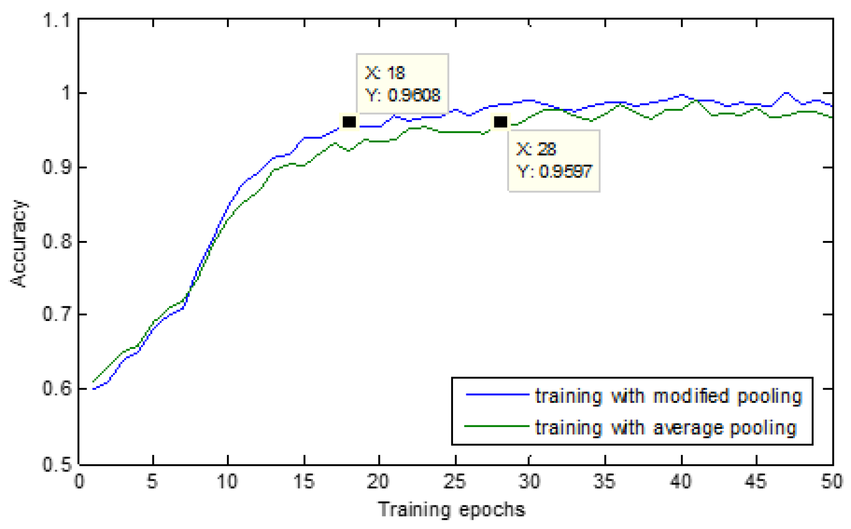
The accuracy curves obtained by the MMBCNN-based detector and classifier are shown in Figure 6 and Figure 7, respectively. Notably, 5/6 of the samples are regarded as training samples, and 1/6 are regarded as test samples. Specifically, the two-branch MMBCNN model is applied. As indicated in Figure 6, the training accuracies of the detection and classification methods stabilize after 20 and 30 epochs, respectively. The convergence speed of the fault detector is higher than that of the fault classifier. Moreover, the optimized model structure can extract distribution network fault features efficiently. We conclude that the MMBCNN with the modified pooling function demonstrates enhanced convergence performance (Figure 7). Compared with the MMBCNN with the average pooling function, the model with the modified pooling function must be trained in fewer epochs to yield the same accuracy.

Figure 6. Overall accuracy curves for the detection and classification models.

Figure 7. Accuracy curves for classification models with various pooling functions.

The structures of the CNN and MMBCNN models adopted in this study are shown in Table 5. The network structure 5C-5P-4C-4P denotes that this CNN contains two pairs of convolution and pooling layers, and the numbers of channels for the first and second C–P pairs are 5 and 4, respectively. Specifically, the second branch, 1C-FC, denotes the 1D CNN and fully connected network. The size of the converted image is critical, as it directly affects feature fidelity and computational efficiency. To identify the optimal dimensions, we compared the average classification accuracies for various image sizes, as shown in Table 6. The results indicate that a size of 16 × 16 pixels yields higher accuracy than other tested resolutions. Therefore, we set the image size to 16 × 16. Table 7 and Table 8 present the performance of the fault detection and classification models using simulation data. For fault detection, the fault detection model is validated through a 2-fold cross-validation. Table 7 indicates that the accuracy of fault detection improves when the parallel branch is added to the CNN model. The highest accuracy obtained by the MMBCNN-based fault detection model is 97%.

Table 5. Structure of various CNN models.

Models	Network Structure	Convolution Kernel Size	Pooling Size
CNN	5C-5P-4C-4P	{5 × 5, 3 × 3}	{2 × 2}
MMBCNN	B1: 5C-5P-4C-4P B2: 1C-FC	{5 × 5, 3 × 3} {1 × 193, 576 × 64}	{2 × 2} —

Table 6. Average classification accuracy with various fault image sizes.

Classifier	MMBCNN
Fault Image Size	12 × 12	16 × 16	32 × 32
Simulation Data	0.972	0.980	0.977
Actual Measurement	0.934	0.957	0.953

Table 7. Comparison of different structures in terms of fault detection.

Methods	CNN			MMBCNN
	F1	F2	AVG	F1	F2	AVG
ACC	0.948	0.948	0.948	0.970	0.970	0.970
REC	0.952	0.933	0.943	0.976	0.947	0.962
PRE	0.980	0.848	0.914	0.985	0.919	0.952
F1	0.966	0.889	0.928	0.980	0.933	0.957

ACC: accuracy, REC: recall, PRE: precision, F1: F1-score, AVG: average.

Table 8. Comparison of different structures in terms of fault classification.

Methods	CNN								MMBCNN
	F1	F2	F3	F4	F5	F6	F7	AVG	F1	F2	F3	F4	F5	F6	F7	AVG
ACC	0.969	0.969	0.969	0.969	0.969	0.969	0.969	0.969	0.980	0.980	0.980	0.980	0.980	0.980	0.980	0.980
REC	0.973	0.963	0.957	0.970	0.977	0.967	0.977	0.969	0.983	0.980	0.973	0.980	0.983	0.980	0.980	0.980
PRE	0.837	0.843	0.847	0.839	0.835	0.841	0.835	0.840	0.889	0.891	0.896	0.891	0.889	0.891	0.891	0.891
F1	0.900	0.899	0.898	0.900	0.900	0.899	0.900	0.899	0.934	0.933	0.933	0.933	0.934	0.933	0.933	0.933

ACC: accuracy, REC: recall, PRE: precision, F1: F1-score, AVG: average.

For fault classification, 7-fold cross-validation is employed, and the results are given in Table 8. The highest accuracy achieved by the MMBCNN-based fault classification model is 98%. Table 8 indicates that the proposed MMBCNN-based model exhibits superior performance in fault classification.

4.2. Effects of the Data Source

This section uses simulation data and real measurements for separate testing to verify the performance of the proposed fault diagnosis model. Table 9 and Table 10 show the detection and classification accuracies of the proposed MMBCNN-based models, respectively. Accuracy is calculated for the estimation of the proposed methods’ performance. The results in Table 9 and Table 10 indicate that the detection and classification accuracies of the MMBCNN model using simulation data are higher than those of the model using actual measurements. This discrepancy arises because measurement data are significantly influenced by the operational state of the distribution network. The quality of on-site fault waveforms is affected by monitoring equipment, leading to indistinct fault characteristics. Additionally, noise interference during real measurement transmission compromises fault classification accuracy. High-impedance grounding faults in actual systems are also particularly susceptible to misclassification.

Table 9. Average detection accuracy with various CNN structures.

Methods	CNN	MMBCNN
Simulation Data	0.948	0.970
Actual Measurement	0.951	0.968

Table 10. Average classification accuracy with various CNN structures.

Methods	CNN	MMBCNN
Simulation Data	0.969	0.980
Actual Measurement	0.932	0.957

4.3. Comparative Analysis of Different Methods

In this section, the proposed method is compared with existing approaches, such as the hidden Markov model, artificial neural network, LeNet-5 CNN [34], 1D CNN [35], and the Transformer model [36]. The simulation data and real measurements are adopted in this test. We divide the training samples into several sets to estimate the accuracy of the detector and classifier. Then, we average the results to ensure the reliability of the test results. Table 11 and Table 12 show that the MMBCNN and the Transformer model have higher fault detection and classification accuracies than the other approaches. However, as shown in Table 13, the Transformer model possesses a significantly larger number of total parameters than the MMBCNN. Correspondingly, the single-image processing latency of the Transformer is also higher than that of the MMBCNN. Therefore, the Transformer model exhibits certain limitations in computing efficiency and in the number of model parameters.

Table 11. Comparison of different methods in terms of fault detection accuracy.

Methods	HMM	ANN	LeNet-5 CNN	1D CNN	Transformer	MMBCNN
Simulation Data	0.866	0.910	0.948	0.957	0.979	0.970
Actual Measurement	0.850	0.897	0.932	0.943	0.969	0.957

Table 12. Comparison of different methods in terms of fault classification accuracy.

Methods	HMM	ANN	LeNet-5 CNN	1D CNN	Transformer	MMBCNN
Simulation Data	0.871	0.921	0.969	0.971	0.986	0.980
Actual Measurement	0.865	0.907	0.951	0.964	0.979	0.968

Table 13. Comparison of different methods in terms of model complexity.

Methods	Transformer	MMBCNN
Total parameters	0.660 M	0.050 M
Latency	1.673 ms	0.211 ms

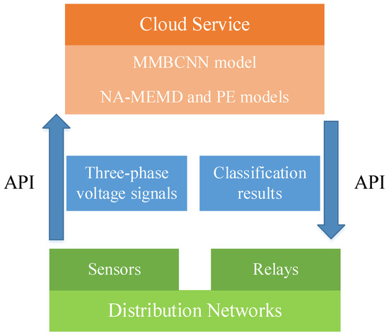
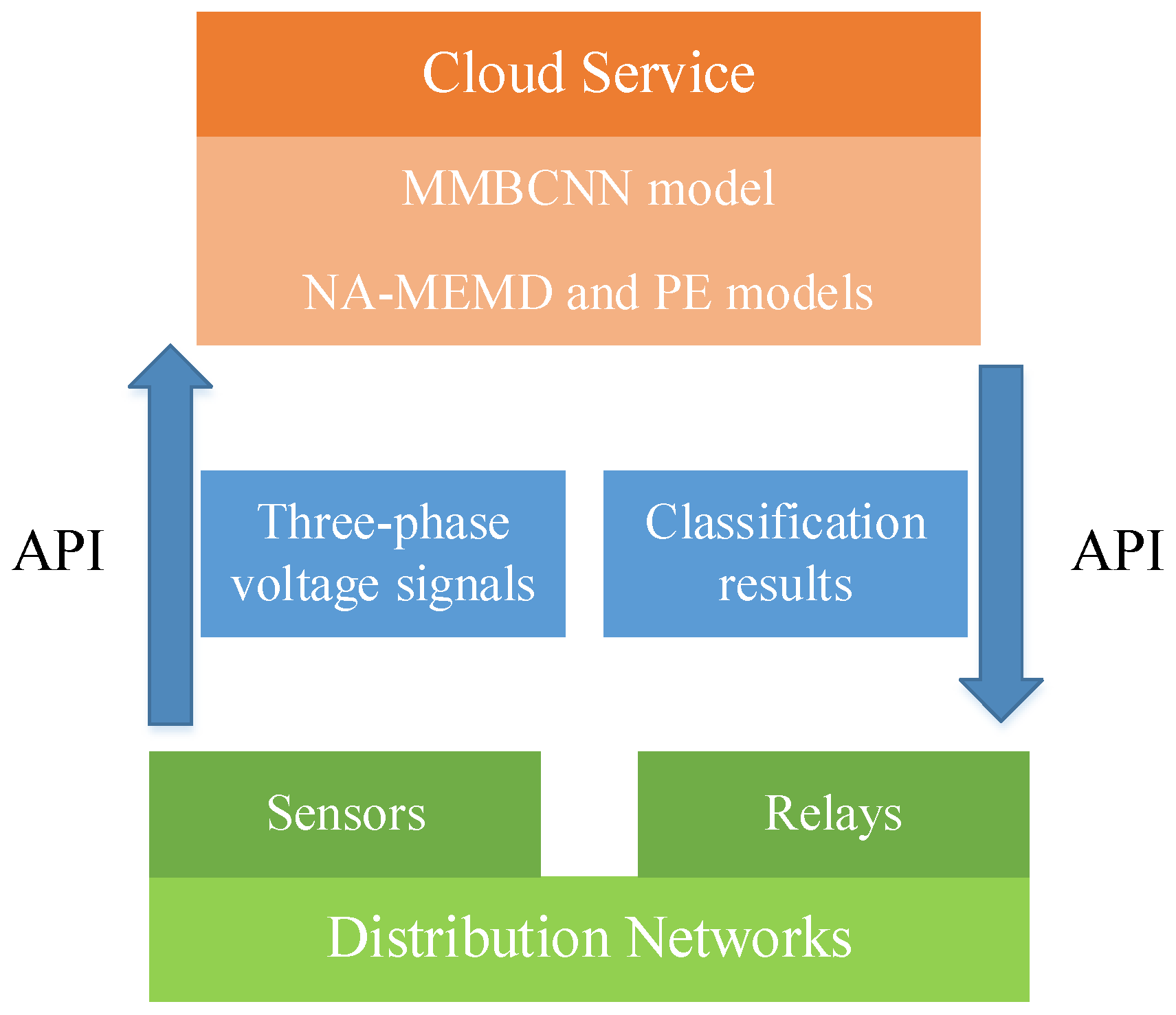
The proposed fault classification model can be deployed in real-world distribution networks utilizing cloud AI techniques, as shown in Figure 8. The data preprocessing module and trained MMBCNN models can be hosted on cloud services such as Alibaba Cloud or Google Cloud. Three-phase voltage signals measured by sensors can then be transmitted to these models via an application programming interface (API), with the prediction results relayed back to the distribution network relays. Depending on application requirements, signal data can be sent in batches for offline prediction or in streams for online prediction.

Figure 8. Actual deployment plan of the MMBCNN model.

5. Conclusions

Feed line faults in distribution networks affect the quality of the user’s power supply and damage power system equipment. This study proposes a novel method based on NA-MEMD and MMBCNN to detect distribution network fault events. Specifically, a moving time window technique combined with the NA-MEMD method is employed to remove noise from high-frequency sampling signals and long-term series signals. The Clarke transform is used to convert transient voltage signals into the d–q axis, and an MMBCNN is employed to detect and classify feed line faults.

The following conclusions are drawn from the case studies. (i) The adaptive adjustment factor incorporated in PE effectively facilitates the elimination of diverse noise components. The signal-to-noise ratio, energy ratio, and standard deviation were specifically designed as indicators to evaluate the NA-MEMD and PE methods. (ii) A modified pooling function was proposed to enhance the model’s convergence performance. (iii) Among the compared approaches, the proposed MMBCNN-based method achieves superior detection and classification accuracies (97% and 98%, respectively), attributable to its parallel branches that enable feature extraction at multiple scales. Although the Transformer model exhibits the highest fault detection and classification accuracies, it underperforms the proposed method in terms of computational efficiency and parameter count.

Feature extraction techniques and the source of fault data are key factors significantly influencing fault classification accuracy. To address these challenges, future research will focus on two primary areas: first, enhancing the model’s capacity to learn more complex and abstract features by incorporating squeeze-and-excitation modules or other attention mechanisms. Second, improving the model’s robustness in real-world applications by accounting for the complexities of actual operational conditions and data quality issues.

References

- Shi, Q.; Liu, W.; Zeng, B.; Hui, H.; Li, F. Enhancing distribution system resilience against extreme weather events: Concept review, algorithm summary, and future vision. Int. J. Electr. Power Energy Syst. 2022, 138, 107860. [Google Scholar] [CrossRef] [Scilit]
- Xiao, F.; Lu, T.; Wu, M.; Ai, Q. Maximal overlap discrete wavelet transform and deep learning for robust denoising and detection of power quality disturbance. Gener. Transm. Distrib. IET 2019, 14, 140–147. [Google Scholar] [CrossRef] [Scilit]
- Han, T.; Wang, X.; Guo, J.; Chang, Z.; Chen, Y. Health-aware joint learning of scale distribution and compact representation for unsupervised anomaly detection in photovoltaic systems. IEEE Trans. Instrum. Meas. 2025, 74, 3538811. [Google Scholar] [CrossRef] [Scilit]
- Nouri, H.; Alamuti, M.M. Comprehensive distribution network fault location using the distributed parameter model. IEEE Trans. Power Deliv. 2011, 26, 2154–2162. [Google Scholar] [CrossRef] [Scilit]
- Li, J.; Gao, M.; Liu, B.; Gao, F.; Chen, J. Fault location algorithm in distribution networks considering distributed capacitive current. IEEE Trans. Power Deliv. 2020, 36, 2785–2793. [Google Scholar] [CrossRef] [Scilit]
- Pang, Q.; Wang, Y.; Wang, Y.; Cao, T. Earth fault location for non-directly grounded distribution networks. IEEE Trans. Power Deliv. 2024, 39, 706–717. [Google Scholar] [CrossRef] [Scilit]
- Li, P.; Zhang, H.; Xiang, H.; Jia, Q. A fast adaptive S-transform for complex quality disturbance feature extraction. IEEE Trans. Ind. Electron. 2022, 70, 5266–5276. [Google Scholar] [CrossRef] [Scilit]
- Lin, C.; Gao, W.; Guo, M.-F. Discrete wavelet transform-based triggering method for single-phase earth fault in power distribution systems. IEEE Trans. Power Deliv. 2022, 34, 2058–2068. [Google Scholar] [CrossRef] [Scilit]
- Cai, K.; Cao, W.; Aarniovuori, L.; Pang, H.; Lin, Y.; Li, G. Classification of power quality disturbances using Wigner-Ville distribution and deep convolutional neural networks. IEEE Access 2019, 7, 119099–119109. [Google Scholar] [CrossRef] [Scilit]
- Huang, J.; Hu, X.; Geng, X. An intelligent fault diagnosis method of high voltage circuit breaker based on improved EMD energy entropy and multi-class support vector machine. Electr. Power Syst. Res. 2011, 81, 400–407. [Google Scholar] [CrossRef] [Scilit]
- Biswal, M.; Prasad, C.D.; Ray, P.; Kishor, N. Modified complete ensemble empirical mode decomposition based HIF detection approach for microgrid system. Int. J. Electr. Power Energy Syst. 2022, 141, 108254. [Google Scholar] [CrossRef] [Scilit]
- Shaik, M.; Shaik, A.G.; Yadav, S.K. Hilbert–Huang transform and decision tree based islanding and fault recognition in renewable energy penetrated distribution system. Sustain. Energy Grids Netw. 2022, 30, 100606. [Google Scholar] [CrossRef] [Scilit]
- Mishra, D.P.; Ray, P. Fault detection, location and classification of a transmission line. Neural Comput. Appl. 2018, 30, 1377–1424. [Google Scholar] [CrossRef] [Scilit]
- Mishra, D.P.; Samantaray, S.R.; Joos, G. A combined wavelet and data-mining based intelligent protection scheme for microgrid. IEEE Trans. Smart Grid 2016, 7, 2295–2304. [Google Scholar] [CrossRef] [Scilit]
- Shukla, S.K.; Koley, E.; Ghosh, S. DC offset estimation-based fault detection in transmission line during power swing using ensemble of decision tree. IET Sci. Meas. Technol. 2019, 13, 212–222. [Google Scholar] [CrossRef] [Scilit]
- Xiong, J.; Liu, M.; Li, C.; Cen, J.; Zhang, Q.; Liu, Q. A bearing fault diagnosis method based on improved mutual dimensionless and deep learning. IEEE Sens. J. 2023, 23, 18338–18348. [Google Scholar] [CrossRef] [Scilit]
- Zhang, X.; Yan, S.; Wang, C.; Han, T. Generalizable fault diagnosis under distribution shifts induced by unseen working conditions via synthetic and adversarial sample learning. IEEE Trans. Reliab. 2025, 74, 5517–5530. [Google Scholar] [CrossRef] [Scilit]
- Hou, S.; Guo, W. Fault identification method for distribution network based on parameter optimized variational mode decomposition and convolutional neural network. IET Gener. Transm. Distrib. 2022, 16, 737–749. [Google Scholar] [CrossRef] [Scilit]
- Zhang, Q.; Ma, W.; Li, G.; Ding, J.; Xie, M. Fault diagnosis of power grid based on variational mode decomposition and convolutional neural network. Electr. Power Syst. Res. 2022, 208, 107871. [Google Scholar] [CrossRef] [Scilit]
- Rai, P.; Londhe, N.D.; Raj, R. Fault classification in power system distribution network integrated with distributed generators using CNN. Electr. Power Syst. Res. 2021, 192, 106914. [Google Scholar] [CrossRef] [Scilit]
- de Bruin, T.; Verbert, K.; Babuska, R. Railway track circuit fault diagnosis using recurrent neural networks. IEEE Trans. Neural Netw. Learn. Syst. 2017, 28, 523–533. [Google Scholar] [CrossRef] [Scilit]
- Jiang, G.; He, H.; Yan, J.; Xie, P. Multiscale convolutional neural networks for fault diagnosis of wind turbine gearbox. IEEE Trans. Ind. Electron. 2018, 66, 3196–3207. [Google Scholar] [CrossRef] [Scilit]
- Jiang, Y.; Xia, L.; Zhang, J. A fault feature extraction method for DC–DC converters based on automatic hyperparameter-optimized 1-D convolution and long short-term memory neural networks. IEEE J. Emerg. Sel. Top. Power Electron. 2021, 10, 4703–4714. [Google Scholar] [CrossRef] [Scilit]
- Wu, J.; Wang, W.; Shang, T.; Cao, J. A novel series arc fault detection method based on CEEMDAN and IFAW-1DCNN. IEEE Trans. Dielectr. Electr. Insul. 2024, 31, 1020–1029. [Google Scholar] [CrossRef] [Scilit]
- Zhang, Z.; Hou, Y.; Yuan, Y. A novel physical information neural network for real-time monitoring and sparse reconstruction of thermal environments with turbulent natural convection in nacelles. Renew. Energy 2025, 240, 122166. [Google Scholar] [CrossRef] [Scilit]
- Rehman, N.U.; Park, C.; Huang, N.E.; Mandic, D.P. EMD via MEMD: Multivariate noise-aided computation of standard EMD. Adv. Adapt. Data Anal. 2013, 5, 1350007. [Google Scholar] [CrossRef] [Scilit]
- Rehman, N.; Mandic, D.P. Multivariate empirical mode decomposition. Math. Phys. Eng. Sci. 2010, 466, 1291–1302. [Google Scholar] [CrossRef] [Scilit]
- Govindarajan, S.; Natarajan, M.; Ardila-Rey, J.A.; Venkatraman, S. Partial discharge location identification using permutation entropy based instantaneous energy features. IEEE Trans. Instrum. Meas. 2021, 70, 6011412. [Google Scholar] [CrossRef] [Scilit]
- Wang, X.; Sun, L.; Lu, C.; Li, B. A novel transformer network with a CNN-enhanced cross-attention mechanism for hyperspectral image classification. Remote Sens. 2024, 16, 1180. [Google Scholar] [CrossRef] [Scilit]
- Lei, Y.; Jia, F.; Lin, J.; Xing, S.; Ding, S.X. An intelligent fault diagnosis method using unsupervised feature learning towards mechanical big data. IEEE Trans. Ind. Electron. 2016, 63, 3137–3147. [Google Scholar] [CrossRef] [Scilit]
- Hu, Y.; Tang, H.; Pan, G. Spiking deep residual networks. IEEE Trans. Neural Netw. Learn. Syst. 2021, 34, 5200–5205. [Google Scholar] [CrossRef] [Scilit]
- Aller, J.; Bueno, A.; Paga, T. Power system analysis using space-vector transformation. IEEE Trans. Power Syst. 2002, 17, 957–965. [Google Scholar] [CrossRef] [Scilit]
- Du, Y.; Liu, Y.; Shao, Q.; Sheng, G.; Jiang, X.; Luo, L. Single line-to-ground faulted line detection of distribution systems with resonant grounding based on feature fusion framework. IEEE Trans. Power Deliv. 2019, 34, 1766–1775. [Google Scholar] [CrossRef] [Scilit]
- Qin, J.; Zhou, B.; Mi, Z. Research of fault diagnosis and location of power transformer based on convolutional neural network. In Proceedings of the 2019 IEEE Innovative Smart Grid Technologies Asia (ISGT Asia), Chengdu, China, 21–24 May 2019; pp. 3589–3594. [Google Scholar]
- Zhang, L.; Sheng, G.; Hou, H.; Jiang, X. A fault diagnosis method of power transformer based on cost sensitive one-dimensional convolution neural network. In Proceedings of the 2020 5th Asia Conference on Power and Electrical Engineering (ACPEE), Chengdu, China, 4–7 June 2020; pp. 1824–1828. [Google Scholar]
- Mogan, J.N.; Lee, C.P.; Lim, K.M.; Ali, M.; Alqahtani, A. Gait-CNN-ViT: Multi-model Gait Recognition with Convolutional Neural Networks and Vision Transformer. Sensors 2023, 23, 3809. [Google Scholar] [CrossRef] [Scilit]
Disclaimer/Publisher’s Note: The statements, opinions and data contained in all publications are solely those of the individual author(s) and contributor(s) and not of MDPI and/or the editor(s). MDPI and/or the editor(s) disclaim responsibility for any injury to people or property resulting from any ideas, methods, instructions or products referred to in the content. |
© 2026 by the authors. Licensee MDPI, Basel, Switzerland. This article is an open access article distributed under the terms and conditions of the Creative Commons Attribution (CC BY) license.