


Abstract
This study examines the methodological landscape and empirical trends in energy elasticity estimation, reviewing literature published from 2017 to 2026. It employs a hierarchical taxonomy to categorize the selected articles by functional form (production, cost, and energy demand), model specification (static and dynamic), and data structure (panel and time-series). Key findings include: First, the review distinguishes production, cost, and energy demand function approaches and synthesizes the literature by showing how these approaches are associated with different data structures and econometric modeling strategies. Second, the analysis highlights the prevalent use of econometric techniques, such as Generalized Method of Moment (GMM) and Autoregressive Distributed Lag (ARDL), to effectively address endogeneity and non-stationarity in recent energy data. Finally, the contribution of this study lies in its structured synthesis of diverse econometric methodologies based on specific data characteristics. By providing a structured roadmap that matches estimation techniques with their corresponding data structures, this review offers guidance for researchers and policymakers to ensure robust and reliable energy elasticity estimates in an era of rapid global energy transitions.
1. Introduction
Energy plays a dual role in economic analysis, serving both as a direct source of utility for households and as a key input in firms’ production processes. Accordingly, the estimation of energy price and income elasticities has traditionally been approached from three main perspectives: (i) production function, (ii) cost function, and (iii) energy demand function. Energy production and cost function approaches focus on the technical relationships between energy and other inputs, including capital and labor, while energy demand approaches examine how consumers and firms adjust their energy use in response to changes in prices and income. Understanding these two perspectives is essential in the field of energy economics, as it provides the analytical foundation for evaluating how economic agents respond to price signals, technological change, and policy interventions.
The importance of analyzing production, cost, and energy demand approach-based elasticities extends across several key policy domains. First, from the perspective of climate change mitigation, energy consumption is a primary determinant of emissions. Thus, understanding its responsiveness to shifts in prices, income, and economic activity is essential for effective policy design [1,2]. Similarly, energy elasticity estimates derived from production and cost functions provide an empirical foundation for understanding the industrial or national energy structure [3,4]. Furthermore, by estimating cross-price elasticities among various energy sources, such frameworks offer analytical insights into the energy transition strategies required to address climate change [4,5,6,7,8]. These estimates are critical for evaluating the effectiveness of measures such as carbon pricing and energy efficiency policies [1,9].
Second, energy security has gained renewed importance amid recent geopolitical conflicts that have disrupted global energy supply chains and heightened economic vulnerability to external shocks. Energy supply shocks such as the Russia–Ukraine war and tensions in the Middle East have demonstrated how energy supply disruptions can translate into broader macroeconomic risks [10]. The study of energy elasticities has become increasingly important, as it provides key insights into how households and firms respond to changes in energy availability and prices, thereby supporting the design of effective energy security policies. Third, energy serves as a cornerstone of economic development. Energy demand reflects advancements in living standards and household welfare [11,12,13]. Production and cost function approaches underscore the pivotal role of energy in facilitating industrialization and productivity growth [9,14,15]. As economies develop, the relationship between income growth, industrial output, and energy use changes due to economic conditions, government policy, and technological progress [10,16]. Estimating energy elasticity is essential for anticipating future energy needs and understanding long-term development trajectories.
Despite the long-standing interest in these analyses, the empirical literature faces new challenges arising from rapid structural changes in global energy systems. Ongoing processes of decarbonization, electrification, and digitalization are transforming both consumption patterns and production technologies. These shifts motivate a comprehensive re-examination of existing empirical evidence [17]. Reflecting this necessity, research on energy transition and energy efficiency is being conducted across various fields, including economics and engineering [18,19]. This trend is also reflected in energy elasticity research, where the increasing availability of diverse energy-related data has facilitated the application of various econometric methodologies. Although some review studies examine energy elasticity, they focus on specific economic agents, countries, and energy sources. These studies also tend to concentrate on presenting the estimation results of energy elasticity [20,21,22,23]. Consequently, there remains a notable research gap for a comprehensive review that encompasses diverse datasets and methodologies. A structured organization that links empirical results to their associated methodological frameworks remains relatively limited.
Research on energy elasticity estimation is broadly categorized into production, cost, and energy demand function approaches, which utilize a diverse range of methodologies. Production and cost function approaches frequently employ translog functional forms [3,4,5,6,7,8,9,14,15,24,25,26,27,28,29]. Static models of energy demand estimation commonly employ panel data techniques such as Fixed Effects (FE), Random Effects (RE), Pooled Ordinary Least Squares (POLS), and Common Correlated Effects Mean Group (CCEMG) estimators [11,12,13,30,31,32,33,34,35,36,37,38,39,40,41,42]. In addition, static time-series analyses often incorporate Time-Varying Parameter (TVP) models [10,16,43,44]. Dynamic energy demand models typically rely on panel data approaches such as GMM, ARDL, and FE estimators [1,45,46,47,48,49,50,51,52,53,54,55], while time-series analyses employ a broader set of techniques, including ARDL-type models, Autometrics, and various cointegration-based methods such as Dynamic Ordinary Least Squares (DOLS), Fully Modified Ordinary Least Squares (FMOLS), Canonical Cointegrating Regression (CCR), and Time-Varying Coefficient Cointegration (TVC), as well as Vector Error Correction Models (VECM) and nonlinear specifications such as Non-linear Autoregressive Distributive Lag (NARDL) [56,57,58,59,60,61,62,63,64,65,66,67,68,69]. These approaches are specifically designed to address complex econometric issues, including adjustment dynamics, heterogeneity, and cross-sectional dependence. By accounting for these properties, these models facilitate more accurate estimation. Therefore, this growing diversity raises important questions about model choice, the comparability of results across production, cost, and energy demand approaches, and the consistency of policy interpretation.
The objective of this paper is to provide a structured and integrated review of the literature on energy elasticity estimation. This study applies a hierarchical taxonomy to analyze the existing literature based on functional forms, model specifications, and data structures. Specifically, this review aims to (i) synthesize the methodological evolution of production, cost, and energy demand functions over the past decade, (ii) evaluate how different econometric techniques address the complexities of panel and time-series data, and (iii) derive methodological and policy implications for the estimation of energy elasticities in a rapidly changing energy environment.
The findings of this review reveal that production and cost function studies, which primarily employ the translog functional form, generally report positive output and negative price elasticities. Several studies highlight significant potential between fossil fuels and renewable energy sources. Within energy demand studies, despite the wide range of estimates produced by diverse datasets and methodologies, including FE, TVC, GMM, and ARDL models, consistent patterns emerge across the literature. Price and income elasticities maintain their expected negative and positive signs. Long-run elasticities are found to be more elastic than their short-run counterparts.
The remainder of the paper is structured as follows. Section 2 describes the methodological framework for literature selection and the hierarchical classification system. Section 3 reviews the core methodologies, categorized by functional forms and data characteristics. Section 4 synthesizes the empirical findings from the reviewed studies and conducts a comparative analysis of energy elasticity estimates across different modeling approaches and data structures. Section 5 concludes and suggests directions for future research.
2. Literature Review
2.1. Information Extraction
To identify and classify the extant literature on energy elasticity based on specific data categories and analytical methodologies, the data categories encompass the subjects of analysis (economic agents), energy sources, and the research’s spatial and temporal scopes. Economic agents are categorized into total (country or region) or specific agents, such as household, industry. Energy sources consist of total energy consumption and specific sources, including electricity, natural gas, oil, gasoline, and coal. Furthermore, the spatial scope is divided into multi-country studies and single-country analyses. The structured process of identification, screening, and classification employed in this study is illustrated in Figure 1.
Figure 1.
Methodological framework for the study selection and classification.
Given the diverse range of categories and methodologies in energy elasticity research, a comprehensive search was conducted using Web of Science (WoS) and Google Scholar. The search strategy involved a combination of core keywords: energy, production function, cost function, energy demand function, price elasticity, income elasticity, and output elasticity. To capture a broad spectrum of research domains, additional keywords such as electricity, gas, oil, gasoline, coal, household, and industry were utilized. The search was restricted to the title, abstract, and keyword lists of the publications.
The scope of the review was limited to articles published over the past decade (2017–2026). While energy elasticity has been a long-standing subject of economic inquiry, this study focuses on recent literature to reflect structural shifts in energy consumption patterns driven by rapid global changes, such as climate change mitigation policies and heightened energy security concerns. Under these criteria, the literature search was finalized in February 2026. Due to the high volume of search results, a rigorous screening process was implemented to ensure relevance. Articles were primarily selected based on their methodological frameworks, specifically, whether they employed production, cost, or energy demand function approaches. This process resulted in a final set of 61 articles for in-depth review after removing duplicate entries identified across databases or multiple versions of the same study, excluding papers that did not explicitly report empirical values for energy elasticity, and excluding incomplete or non-peer-reviewed research materials such as doctoral dissertations, master’s theses, and conference proceedings.
The selected studies underwent a two-stage hierarchical classification to analyze the distinct features of energy elasticity estimation. In the first stage (Classification 1), the studies were categorized by their functional form into either production and cost functions (n = 15) or energy demand functions (n = 46). As both cost and production functions are production-side approaches, they are presented in a single category. While the review considers both approaches, it classifies the literature separately into two approaches and applies additional classification to the energy demand literature given its greater methodological diversity. In the second stage (Classification 2), the 46 energy demand studies were further classified based on their model specification into static models (n = 20) and dynamic models (n = 26). Each of these categories was then subdivided by data structure, distinguishing between panel data and time-series data. Consequently, this study structurally organizes the literature according to functional forms, econometric specifications, and data characteristics to provide a comprehensive overview of the current research landscape.
2.2. Literature on Production and Cost Function Approaches
A total of fifteen studies employ production- or cost-theory frameworks to estimate energy substitution and elasticity parameters. The primary objective of these studies is to provide robust empirical parameters essential for the design and calibration of energy-oriented computable general equilibrium (CGE) models, thereby enhancing the accuracy of policy simulations such as carbon taxes or renewable energy subsidies.
First, twelve studies adopted a translog production function framework. Within this group, ridge regression is predominantly employed to address severe multicollinearity arising from interaction and squared terms [5,6,7,9,14,15,24,25,26,27,28,42]. The translog production function literature primarily examines energy substitution possibilities and output elasticities across both emerging and developed economies. These studies typically model industrial production structures in which energy is treated as a core input alongside capital and labor. To mitigate the multicollinearity inherent in translog specifications due to the large number of parameters, most studies rely on ridge regression rather than Ordinary Least Squares (OLS) to obtain stable and reliable estimates.
Bello and Solarin [24] and Li et al. [6] use a ridge trace plot to select an optimal penalty parameter for the U.S. and China, respectively. Lin and Liu [9] analyze China’s heavy industry, focusing on interactions among energy, capital, and labor to identify energy-saving pathways. Similarly, Hou and Song [25] decompose China’s energy inputs into thermal power, clean energy, and fossil fuels to investigate the role of directed technical change in facilitating energy transition. Notably, Faizi and Mohammad [3] also incorporate GMM methodology with ridge regression to resolve endogeneity issues in their dynamic panel analysis. They employ manufacturing industry data for India, highlighting substitutability between labor and capital while identifying complementarity between energy and non-energy inputs.
Studies focusing on renewable energy transition within this framework often differentiate between clean and traditional sources. Lin and Ankrah [7] and Wesseh and Lin [15] examine the substitution potential in Nigeria and Egypt, respectively, by estimating the possibilities of switching from non-renewable electricity and fossil fuels to renewable energy sources. In Tunisia, Saadaoui and Chtourou [28] assess the role of renewable energy in shaping the national energy transition, incorporating conventional production factors to qualify the economic impact of decarbonization. Solarin and Bello [14], focusing on Brazil, introduce a sustainability index (Adjusted Net Savings) alongside GDP to provide a more robust assessment of the substitution between biomass and fossil fuels. For Pakistan, Khalid and Jalil [5] analyze inter-fuel substitution among coal, natural gas, petroleum, and hydroelectricity, finding that hydroelectricity exhibits the highest output elasticity. Raza and Tang [27] extend this analysis by incorporating labor and capital inputs, estimating the carbon mitigation potential of transitioning toward natural gas and electricity under alternative investment scenarios. Lin and Atsagli [26] investigate South Africa and find that coal and electricity remain the primary drivers of output, accompanied by relatively faster technological progress compared to petroleum.
Second, the remaining three studies employ translog cost function frameworks [4,8,29]. They model firm behavior under cost minimization, with a focus on industrial fuel substitution. Unlike production-theory approaches that primarily rely on input quantities, these studies emphasize price responsiveness and derive demand elasticities that satisfy neoclassical regularity conditions, including positivity, monotonicity, and curvature. Although all three studies adopt variants of the translog cost system, they differ in their estimation techniques and data structures.
Using Full Information Maximum Likelihood (FIML), Javid [4] analyzes Saudi Arabia’s industrial sector, explicitly accounting for contemporaneous correlations among disturbances and imposing essential regularity conditions like local concavity directly during estimation. With nonlinear regression systems (NLSs), thereby ensuring theoretical consistency with cost minimization, Mardones and Henríquez [8] examine the Chilean industrial sector. Xiao et al. [29] apply a restricted cost function (RCF) estimated via seemingly unrelated regression (SUR), treating renewable energy as a quasi-fixed input to address limitations associated with market-based renewable energy prices. They analyze China’s low-carbon transition. By treating renewable energy as a quasi-fixed input, they address the lack of reliable provincial-level price data for wind and solar energy. Their model is estimated using SUR to account for correlations across 27 Chinese provinces and incorporates a vector angle method to capture a non-linear, U-shaped relationship among substitution elasticities in the energy transition process.
The literature on production and cost function approaches demonstrates distinct methodological preferences dictated by specific research objectives and data availability. Most production function studies employ ridge regression to mitigate the multicollinearity inherent in flexible translog specifications, thereby facilitating the estimation of output elasticities. In contrast, cost function frameworks utilize techniques such as FIML and NLS to derive price elasticities. These methodological choices align with specific research objectives, as the production function approach evaluates energy’s contribution to the national economy while the cost function approach identifies the price responsiveness of individual energy sources and industrial sectors.
2.3. Literature on Energy Demand Function Approach
2.3.1. Literature on Static Models
A total of twenty studies is identified as adopting static approaches to estimate energy demand functions. This group is further classified based on data structure.
First, sixteen studies employ panel data. Within the panel data, researchers primarily rely on FE [11,12,13,32,33,34,35,37,38,39,40,41,42], POLS [31], and CCEMG estimators [30,36]. The first thirteen studies employ panel data to examine national or regional energy demand elasticities using FE models. Burke and Kurniawati [33] apply an FE model to regional data from Indonesia, accounting for province-specific characteristics by incorporating population, diesel prices, and average temperature as control variables. Saha and Bhattacharya [39] distinguish electricity consumers in West Bengal into the agricultural, commercial, and industrial sectors to capture heterogeneous consumption behavior. For rural coal demand in China, Teng et al. [40] consider the effects of climate variables, such as average winter temperatures.
Similarly, Su [13] analyzes Taiwan’s electricity sector and confirms the superiority of the FE model over the POLS and RE models through Hausman tests. The study incorporated control variables, including air conditioner ownership and cooling degree days, to enhance the precision of the estimation. Yu and Xin [41] examine China’s electricity sector, accounting for the impact of electricity system reform as a key control variable. Their findings revealed sectoral differences, showing that an FE structure was suitable for the industrial sector, whereas an RE model better represented the residential sector. The analysis of micro-level and household consumption behavior also extensively utilizes FE models to control socio-economic factors. Studies by Chindarkar and Goyal [35] and Boogen et al. [32] analyze residential electricity demand in India and Switzerland, respectively, by incorporating household-level characteristics. Chindarkar and Goyal [35] control for household size and urban location. Similarly, Boogen et al. [32] utilize a comprehensive set of control variables, such as household size, single-person household status, housing tenure, number of rooms, and whether children are present in the household.
To mitigate endogeneity issues, particularly with respect to energy prices, several studies employ instrumental variable (IV) approaches within FE frameworks. Caldara et al. [34] utilize changes in global oil production as an instrument for crude oil prices across OECD countries, while Alberini et al. [11] address the endogeneity between marginal prices and natural gas consumption in Ukraine using tariff-based instruments. Lanot and Vesterberg [38] analyze hourly electricity demand in Sweden, instrumenting prices with the logit-estimated probability of consumption exceeding specific thresholds. For China, Zhai et al. [42] address electricity price endogeneity by employing coal price volatility and power generation scale as supply-side instruments. Similarly, Kilian and Zhou [37] utilize U.S. state-level gasoline price pass-through rates and international price shocks as instruments for gasoline prices.
Alternative panel structures, such as pseudo-panels and the CCEMG estimator, have been adopted to address data limitations and complex cross-sectional dependencies. Belaïd et al. [12] and Bardazzi and Pazienza [31] employ pseudo-panel methods by constructing cohorts from repeated cross-sectional data to analyze residential energy demand elasticity in France and Italy, using FE and POLS models, respectively. To address cross-sectional dependence and slope heterogeneity, Dong et al. [36] employ the CCEMG estimator to analyze natural gas demand in China, allowing for province-specific coefficients while controlling for unobserved common factors. Similarly, AlKathiri et al. [30] estimate energy income elasticity for 111 countries using the CCEMG estimator.
The remaining four studies focus on time-series analysis, primarily utilizing TVP models to capture the evolution of price and income elasticities over time [10,16,43,44]. Unlike models that assume constant parameters, this approach accounts for the dynamic nature of energy markets by allowing elasticities to adjust in response to changing economic and environmental conditions. These studies commonly apply the Kalman filter to track the time-varying trajectories of parameters by recursively updating coefficients as new information becomes available.
Wang and Mogi [44] utilize this approach to analyze Japan’s industrial and residential electricity demand, examining how structural shocks, such as the Fukushima nuclear accident, alter consumer responsiveness. Similarly, Tiwari and Menegaki [43] examine India’s electricity demand by incorporating macroeconomic controls, including foreign direct investment and export-to-GDP ratios, to identify trends in price and income elasticities. Lee and Olasehinde-Williams [10] also applied the Kalman Filter to estimate gasoline demand elasticities across five major energy-consuming nations (China, India, USA, Russia, and Japan), providing a comparative analysis of parameter trends and country-specific responsiveness. In South Africa, Masike and Vermeulen [16] utilized a TVP to capture fluctuations in electricity demand elasticities driven by external factors, such as changes in electricity tax policy.
The review of static energy demand models reveals a clear methodological divergence driven by data characteristics. While panel-based studies prioritize controlling for unobserved heterogeneity, time-series approaches emphasize the time-varying nature of elasticities. By adopting Kalman filter-based TVP models, the latter capture the sensitivity of economic agents to structural breaks and external shocks, reflecting ongoing efforts to incorporate temporal dynamics within an otherwise static functional framework. While static approaches offer insights into contemporaneous relationships, the gradual adjustment of the energy market over time is not captured. This limitation motivates the adoption of dynamic models, which account for the time lags and intertemporal adjustment processes necessary for the energy market to reach equilibrium.
2.3.2. Literature on Dynamic Models
Unlike static models, dynamic models incorporate lagged dependent variables as regressors to capture the persistence of energy consumption and intertemporal adjustment processes. Twenty-six studies are identified in this category; twelve studies employ panel data and fourteen studies use time-series analysis.
First, among the twelve panel data studies, five studies apply GMM to mitigate the endogeneity inherent in dynamic specifications [1,45,46,50,55]. Cialani and Mortazavi [46] and Csereklyei [1] apply system GMM methodology to estimate electricity demand elasticity across EU member states, with the latter incorporating environmental tax revenues as a control variable to reflect the impact of green policies. For OECD industrial sectors, Chang et al. [45] utilize both difference and system GMM, comparing the disparity of elasticities between energy-intensive and non-intensive industries. A more detailed analysis of a specific industry was provided by Wakashiro [55], who used difference GMM to estimate the electricity price elasticity of Japan’s manufacturing sector while accounting for prefecture-specific effects. Kostakis and Lolos [50] estimate the electricity demand elasticity of Greek households using a pseudo-panel.
Another five studies adopt the ARDL models to address long-run dynamics and cross-sectional heterogeneity [47,48,51,52,53], and the remaining two papers rely on FE estimators [49,54]. Liddle and Huntington [52] and Liddle and Hasanov [51] employ Mean Group (MG) and Dynamic Common Correlated Effects (DCCE) estimators across global panels to control unobserved common factors and country-specific differences, focusing on aggregate energy and electricity, respectively. This approach was also mirrored by Liddle et al. [53] in their analysis of 26 middle-income countries. In European natural gas markets, Erias and Iglesias [47,48] adopt ARDL models to investigate seasonal variations and the structural impact of the COVID-19 pandemic, employing monthly data and country-specific dummies to examine differences across seasons and countries.
Two other studies utilize FE models, often incorporating instrumental variables or bias-corrected methods to ensure consistency in dynamic settings [49,54]. Gao et al. [49] address the endogeneity of price and income by utilizing their lagged values as instruments within an FE, facilitating a comparative assessment of 65 countries across different income levels. Similarly, focusing on electricity and natural gas consumption, Priesmann and Praktiknjo [54] adopt a bias-corrected method for German household data.
Second, regarding fourteen time-series studies, ARDL models are the most widely used, accounting for eight studies [56,57,58,59,61,67,68,69]. Atalla et al. [58] and Alarenan et al. [56] investigate industrial demand elasticity in Saudi Arabia by incorporating structural trends and export factors into their ARDL specifications, focusing on gasoline and total energy, respectively. Similarly, Campbell [59] and Ishaque [61] scrutinize sectoral electricity demand in Jamaica and Pakistan, respectively, utilizing demographic controls to estimate energy consumption. Campbell [59] uses the urban population share as demographic control, whereas Ishaque [61] employs the number of electricity consumers. Tatli and Barak [69] apply this methodology to investigate coal demand in Turkey, highlighting its efficacy for limited sample sizes while incorporating climatic factors as essential control variables, including average temperature. Raghoo and Surroop [67] apply the ARDL approach to Mauritius, addressing restricted time-series observations while examining specific energy sources, including gasoline, diesel, and fuel oil. Alzyadat [57] estimate the price and income elasticities of natural gas in Saudi Arabia. To account for rapidly increasing domestic energy demand, this study incorporated population growth as a key control variable. Similarly, Taghvaee et al. [68] analyze Iran’s five energy sources (natural gas, diesel, fuel oil, kerosene, and LPG). To reflect Iran’s unique economic characteristics, energy efficiency, exchange rates, and subsidies are used as control variables, with energy efficiency measured as GDP per energy consumption.
In addition, two studies employ Autometrics [62,66]. Recently, variable selection methodologies have been developed to identify necessary variables for analysis, and one such approach, Autometrics, is being utilized to estimate energy demand elasticities. Pellini [66] and Li et al. [62] apply the Autometrics algorithm to identify relevant indicators and dummy variables for EU household electricity demand. These studies incorporate cooling degree days and heating degree days as control variables. For the estimation, specific year dummy variables are selected from the full set of observations based on the Autometrics methodology.
The remaining studies utilize a range of specialized econometric models, including DOLS [64], FMOLS [64], CCR [64], TVC Cointegration [65], VECM [60], and NARDL [63]. Mikayilov et al. [64] applied a triad of DOLS, FMOLS, and CCR models to analyze Turkish gasoline demand elasticity. Mikayilov et al. [65] adopt TVC Cointegration to estimate shifting elasticity for gasoline demand in Azerbaijan. For Brazilian residential electricity, Gutiérrez and Ehrl [60] implement a VECM to account for the long-term equilibrium between consumption, appliance penetration, and climate fluctuations, checking the model choice through identified cointegrating vectors. Liao et al. [63] adopt the NARDL models to demonstrate asymmetric elasticity in energy demand in Taiwanese households, where price elasticities differ between periods of price appreciation and depreciation. This approach provides a more granular representation of consumer sensitivity by capturing the non-linear nature of price elasticities.
Dynamic energy demand research effectively bridges the gap between past consumption habits and future policy planning by identifying long-run equilibrium relationships. While panel-based studies primarily focus on managing endogeneity and cross-sectional dependency through GMM and ARDL, time-series analysis emphasizes the robust identification of cointegrating relationships. The evolution toward incorporating asymmetric responses and automated selection signifies an ongoing refinement in the methodological landscape to enhance the precision and sophistication of elasticity estimates.
In summary, the diverse methodology of energy elasticity estimation is organized according to research objectives and data structures. Production and cost function approaches utilize flexible translog specifications to identify technical substitution possibilities and the contribution of energy to national output. Energy demand function approaches focus on the economic responsiveness of various economic agents, energy sources, and countries, while static panel and time-series models prioritize either unobserved heterogeneity or temporal instability, and dynamic approaches such as GMM and ARDL cover the short run and long run. This hierarchical categorization demonstrates that the selection of econometric techniques is a deliberate effort to match the complexity of energy consumption behavior with the identification strategy available for a given data structure.
3. Estimation Model Specifications
3.1. Production and Cost Function
The production process is characterized by an aggregate production function where output is determined by primary inputs, specifically capital (K), labor (L), and energy (E) [70,71]. This fundamental relationship, assuming a constant state of technology over time, is expressed in Equation (1) as follows. represents the total output of the sector or economy, and , , and denote the inputs of capital, labor, and energy at time t, respectively.
To facilitate empirical estimation, the functional relationship in Equation (1) is represented in a log-linear form. This basic specification, which provides a first-order approximation of the production relationship, is presented in Equation (2) [3,9,28].
From this log-linear function, the objective is to estimate the output elasticities with respect to factor inputs. In this specification, represents the intercept and denotes the error term. The coefficients , , and signify the output elasticities of capital (), labor (), and energy (), respectively.
The basic log-linear model in Equation (2) does not capture the complex interdependencies between production factors. To overcome these restrictions and specifically to examine the cross elasticities among capital, labor, and energy, the model is extended into a transcendental logarithmic (translog) production function. By adding squared terms of each input and their interaction terms into the linear specification, the translog model is expressed in Equation (3) [7,9].
In this specification, the coefficients , , and denote the squared terms for capital, labor, and energy, respectively. Additionally, , and are the coefficients for the interaction terms between these inputs. Cross elasticity is defined as the percentage change in the ratio of input factors in response to a relative change in the marginal rate of technical substitution, assuming that both technology and factor prices remain constant. Based on the estimated coefficients from Equation (3), the cross elasticity (Equation (4)) between energy, capital, and labor are empirically estimated. , , and are the cross elasticities between capital and labor, capital and energy, and labor and energy, respectively. These parameters enable the determination of whether energy functions as a substitute or a complement to other inputs. The derivation of Equation (4) from Equation (3) follows the methodology described in Section 2.1 of Lin and Liu [9]. The sign of the cross elasticity values identify the relationship between production inputs. A cross elasticity value greater than zero indicates a substitute relationship between the inputs, whereas a value less than zero signifies a complementary relationship. When the value equals zero, the relationship between the inputs is considered independent.
The cost function originates from the underlying production mechanism, as defined in Equation (5). Here, p represents the vector of factor prices, x is the vector of input quantities, and y denotes the output level. The total cost is derived from the product of factor prices and their corresponding inputs, where the optimal production is identified by minimizing costs under the constraints of the production function.
To facilitate empirical estimation, the cost-minimization problem is expressed in the translog form shown in Equation (6). This functional form includes the logarithms of prices for capital (r), labor (w), and energy (ep), as well as their second-order and interaction terms. , , and are the coefficients for the first-order input price terms, while , , and denote the coefficients for the second-order terms. , , and represent the coefficients for the interaction terms between the input prices. In a manner consistent with the approach used for the production function in Equation (3), this specification enables the estimation of both own-price and cross-price elasticities [4,8].
3.2. Energy Demand Function
Analyzing the determinants of energy consumption and their responsiveness to economic shocks is a fundamental task in energy economics. Specifically, quantifying price and income elasticities is crucial for evaluating the effectiveness of energy policies and forecasting future demand trends. The energy demand function has served as the primary analytical framework in the literature. Equation (7) represents the basic functional form widely adopted to estimate these elasticities [16,33,35,36,40,44].
In this function, the final energy consumption () of a specific country i in year t is determined by the energy price index (), income (), and control variables (), where the i may also represent individual regions, or households, depending on the study. Depending on the specific research objective, control variables may include factors such as policy, population, and climate [1,13,57,62,66]. The energy price and income elasticities can be identified by expressing the energy demand function of Equation (7) as a log-linear relationship, as shown in Equation (8).
In this equation, and represent individual effects and idiosyncratic errors, respectively. The values of and correspond to the energy price and income elasticity, respectively. A function such as Equation (8) corresponds to a static energy demand model. Static models are based on explaining energy consumption behavior at a specific point in time, assuming that economic agents immediately adjust their energy use in response to changes in price, income, and other exogenous factors.
In contrast, dynamic models focus on the fact that energy consumption adjustment does not occur instantaneously but involves a time lag. This reflects the reality that final energy consumption cannot immediately move to an equilibrium point due to technological and institutional characteristics of energy market [45]. Therefore, dynamic models account for the time required for final energy consumption to reach equilibrium. Equation (9) is a method utilized by various studies to reflect the time lag in energy market equilibrium [1,46,55,58,62,68]. It indicates that the actual change in energy consumption in a specific period () is a certain proportion () of the desired change in consumption ().
Equation (9) is rearranged to express the actual energy consumption as shown in Equation (10). The desired level of energy consumption () is assumed to be a function of energy prices, income, and other control variables, as specified in Equation (11). By substituting Equation (11) into Equation (10) and rearranging the terms, the dynamic energy demand function is derived in a linear logarithmic form as shown in Equation (12).
In Equation (12), the coefficients for the energy price and income variables are the short-run price () and income () elasticities, respectively. The coefficient for the lagged final energy consumption () indicates the degree to which a shock to the dependent variable has a persistent effect on that variable. When the absolute value of this coefficient is less than 1, the long-run elasticities for energy price and income (, ) are derived according to Equations (13) and (14). If the value of the lagged dependent variable coefficient exceeds 1, shocks to energy consumption do not converge to zero over time, implying non-stationary adjustment dynamics.
3.2.1. Static Models
Within the static model, three methodologies are usually utilized to estimate energy elasticities: FE, CCEMG for panel data analysis, and TVP models for time-series data. First, FE is a panel data estimation method specifically designed to address cases where unobserved individual effects in Equation (8) are correlated with the independent variables. In the energy demand, these individual effects represent region-specific or category-specific characteristics that remain constant over time but are not explicitly captured in the data. If these individual effects are correlated with price or income, a standard POLS regression would yield biased and inconsistent estimates of the elasticities [72]. The FE model resolves this by controlling for these persistent individual effects, allowing for the accurate estimation of the coefficients and in Equation (8), which represent the price and income elasticities of energy demand. To statistically validate this approach, researchers typically employ the Hausman test to determine whether the individual effects are correlated with the regressors, thereby justifying the selection of the FE model over the random effects (RE) model to ensure the consistency of the estimated coefficients.
Second, CCEMG is a robust panel estimator designed to address cross-sectional dependence and slope heterogeneity, which can otherwise lead to inconsistent estimates and misleading conclusions in energy demand analysis. This method accounts for unobserved common shocks including global economic shifts or technological changes by augmenting the regression with cross-sectional averages of the dependent and independent variables. The model is implemented through Equation (15).
Here, , , , and are observables, , , and represents the individual-specific estimates of coefficients, is the unobserved common factor with the heterogeneous factor, and and are the intercept and error term, respectively. The terms , , and represent the cross-sectional averages used to filter out unobserved common factors, ensuring that the CCEMG estimator provides consistent long-run parameters while allowing for structural heterogeneity across different observation units [73].
Third, TVP is utilized to estimate elasticities that evolve over time by moving beyond the restrictive assumption of constant coefficients found in static models. This approach is particularly necessary when analyzing energy markets characterized by structural breaks such as technological shifts or policy reforms which constant elasticity models often fail to capture accurately [43]. By allowing parameters to change at each point in time, the TVP adequately deals with potential instabilities and nonlinearities in the data. The model is typically implemented using a state-space representation and estimated via the Kalman filter. Based on the functional form of Equation (16), the TVP model is specified through an observation equation and a state equation.
where , , .
In the observation equation, , , and represent energy consumption, price, income, and control variables at time t, respectively, while and denote the time-varying price and income elasticities, respectively. The terms and represent the observation and state transition errors, respectively.
3.2.2. Dynamic Models
The estimation of energy elasticity in a dynamic model involves several methodologies based on energy demand functions, particularly GMM and ARDL. GMM is primarily used for panel data analysis, while ARDL is applicable to both panel and time-series data. These two methodologies allow for the estimation of short-run and long-run elasticities and have been frequently adopted in the literature for dynamic modeling.
First, GMM is the primary econometric framework utilized to estimate dynamic energy demand functions. GMM is an estimation that addresses endogeneity bias in dynamic panels by utilizing internal instrumental variables which are specifically lagged values of the regressors to provide consistent and unbiased estimates. The necessity for GMM arises because the inclusion of the lagged dependent variable in Equation (10) introduces a fundamental endogeneity problem. This lagged term is inherently correlated with the time-invariant individual effects (), which cause standard POLS or FE estimators. GMM resolves these issues by employing internal instrumental variables to produce consistent and unbiased estimators.
Within this framework, many studies adopt difference GMM (Arellano and Bond [74]), which transforms the equation into first differences to eliminate individual effects and use lagged levels of the variables as instruments. Alternatively, system GMM is frequently utilized because it combines the equations in both levels and differences into a single system to improve estimation efficiency and mitigate the weak instrument problem [74,75]. Through GMM estimation, the coefficients and represent the short-run price and income elasticities, while the coefficient for the lagged variable is used to calculate long-run elasticities according to the relationships in Equations (13) and (14).
Second, the panel ARDL is a methodology utilized to estimate energy elasticities by incorporating lags of both dependent and independent variables. A standard log-linear ARDL (1, 1, 1) specification is expressed as Equation (17).
In this model, the long-run price and income elasticities (, ) are calculated by Equation (18). The ARDL approach is essential because it reflects the gradual adjustment of energy consumption to economic shocks, accounting for the time required to replace capital or technology [51]. Furthermore, it provides consistent estimates regardless of whether the regressors are stationary I(0) or non-stationary I(1), offering greater flexibility than traditional cointegration methods.
Beyond the scope of panel-based estimations, the time-series ARDL is employed for country-specific energy demand studies. While panel models account for cross-sectional heterogeneity, the time-series ARDL facilitates a more granular analysis of a specific economy’s dynamic adjustment process. A primary advantage of this methodology is its statistical reliability in small sample sizes, rendering it particularly suitable for energy research where long-term historical data sets may be limited [59,67].
4. Estimation Results
4.1. Production and Cost Function Approaches
The empirical evidence from studies employing production and cost theory frameworks, as summarized in Table 1, Table 2, Table 3 and Table 4, reveals several distinct patterns regarding scope, economic agents, and estimated elasticities. First, while some studies address broad economic trends, the majority of the literature focuses on individual countries, covering a diverse range of economies, including China, Saudi Arabia, Chile, India, Pakistan, Egypt, Tunisia, Nigeria, Brazil, and the United States. Second, with respect to economic agents, analyses at the national level are the most fre-quent, although several studies focus on the industrial and manufacturing sectors. Third, although electricity and conventional fossil fuels (coal, oil, and natural gas) remain the primary energy sources of interest, the literature also extensively covers clean and renewable energy sources, including hydroelectric, wind, solar, and biomass.
Table 1.
Estimation results of production function model (output elasticity).
Table 2.
Estimation results of cost function model (price elasticity).
Table 3.
Estimation results of production and cost function model (output—cross elasticity).
Table 4.
Estimation results of production and cost function model (price—cross elasticity).
Fourth, from a methodological standpoint, researchers employ sophisticated functional forms, primarily the translog production function, translog cost function, and RCF. These are estimated using a diverse range of econometric techniques, with ridge regression being the most prevalent method to address severe multicollinearity among interaction terms. Other advanced techniques include FIML utilized for Saudi Arabia to ensure theoretical consistency, SUR for Chinese provincial panels, and NLS applied to Chilean firm-level microdata. Fifth, estimated own-price elasticities are consistently negative across all studies, adhering to economic theory. While industrial demand for fuels in Saudi Arabia is generally price-inelastic—with values for natural gas at −0.40, electricity at −0.13, fuel oil at −0.94, and diesel at −0.17—certain energy sources in Chile exhibit highly elastic behavior, such as electricity (−1.03) and fossil energy (−1.30). In China, traditional energy also shows low responsiveness with an elasticity of −0.53.
Sixth, output elasticities for energy and non-energy factors are typically positive, indicating that increases in input drive production growth. Capital and labor often emerge as primary drivers, as seen in India where capital elasticity is 0.45 and labor is 0.39, and in Egypt where labor stands at 1.72. Specific energy types like hydroelectricity in Pakistan exhibit exceptionally high output sensitivity, with values reaching an average of 0.72. Regarding substitution relationships, most energy pairs exhibit positive elasticities (MES (Morishima Elasticity of Substitution) or AES (Allen-Uzawa Elasticity of Substitution) > 0), indicating substitutability. Strong substitution is found in the US electricity sector between natural gas and clean energy (1.01), and in Egypt between renewable electricity and non-renewable electricity (1.41).
The recurring observation of own-price inelasticity for essential fuels like electricity and diesel reinforces their characterization as indispensable inputs with limited short-term alternatives. This result implies that price-based interventions alone may exert a constrained influence on demand abatement unless accompanied by technological advancements. Although elasticities vary across countries, distinct disparities are evident according to the type of energy source. For instance, the high elasticity of substitution identified between clean and fossil fuels in the US, Saudi Arabia, and Egypt suggests a significant potential for facilitated energy transitions through relative price reforms. However, research also reveals critical structural barriers to energy transition. The significant complementarity of coal with other fuels in China—where natural gas or electricity expansion may paradoxically drive coal use (negative MES)—reveals deep-seated technological dependencies that hinder decarbonization. Similarly, the complementarity between energy and capital/labor in the Indian manufacturing sector (e.g., labor-energy MES of −3.78) suggests that energy shortages could act as a direct bottleneck to industrial returns. In contrast, a non-linear U-shaped relationship identified in China indicates that the positive impact of renewable energy and electricity substitutability for natural gas only intensifies once a specific threshold of market and infrastructure maturity is reached.
Finally, the prevalence of flexible translog frameworks in the literature emphasizes the necessity of allowing for variable substitution and non-linear relationships among multiple inputs. Nevertheless, these models are often static in nature, and while they provide robust evidence of long-term substitution possibilities, they are limited by their inability to fully evaluate the dynamic trajectories or adjustment speeds through which demand responds to sudden economic shocks or rapid technological shifts over time.
4.2. Energy Demand Function Approach
4.2.1. Static Model
- (1)
- Panel Data
The empirical evidence derived from static panel studies reveals common characteristics of elasticities. The estimated price elasticities reported in Table 5 are generally negative and inelastic, with crude oil exhibiting particularly low elasticity. Exceptions to this pattern are observed in two studies: Dong et al. [36] report positive price elasticities (0.35 to 0.52), whereas Teng et al. [40] identify elastic responses (−1.02 to −1.21). Income elasticities are typically positive and inelastic. Again, two studies deviate from this pattern, as Dong et al. [36] find elastic income responses (1.09 to 1.38), while Teng et al. [40] report negative income elasticities (−0.97 to −1.40).
Table 5.
Estimation results of static panel model.
Many static panel studies analyze residential electricity demand. Some studies utilize household-level survey data. The recurring observation of price inelasticity reinforces the characterization of energy as an essential good. This result implies that price-based interventions may exert a constrained influence on demand abatement, as economic agents exhibit minimal flexibility in modifying consumption patterns following price increases. Although elasticities are subject to variations across different countries and economic agents, distinct disparities are evident according to the type of energy source. The price inelasticity of crude oil underscores its indispensable nature relative to other sources. Conversely, the higher elasticity identified for gas suggests greater potential for substitution within energy sources.
The atypical positive price elasticity for Chinese natural gas, as reported by Dong et al. [36], is linked to the unique institutional landscape of the Chinese market, which is defined by rigorous price controls and simultaneous supply expansion. This result demonstrates that price elasticity can be significantly shaped by domestic regulatory frameworks. Furthermore, the negative income elasticity for coal in rural China documented by Teng et al. [40] points to a "fuel switching" phenomenon, where rising incomes enable a transition from coal to cleaner or more efficient energy alternatives. Finally, the prevalence of the fixed-effects framework in the literature emphasizes the necessity of accounting for unobserved heterogeneity at the national or household level. Nevertheless, these static models are limited by their inability to evaluate the dynamic trajectories through which demand responds to economic shocks over time.
- (2)
- Time-Series Data
Empirical results from static time-series studies reveal that while the data characteristics and modeling approaches may differ from those of static panel studies, the characteristics of the estimated elasticities remain consistent. The estimated price elasticities in Table 6 are consistently negative and inelastic, ranging from −0.02 to −0.51. However, the degree of price elasticity varies depending on the specific country, economic agent, and energy source. Lee and Olasehinde-Williams [10] found that gasoline demand across five major economies exhibited consistently low-price elasticities. Income elasticities are generally positive, though their magnitudes differ across studies. Wang and Mogi [44] identified an elastic income response of 1.45 for Japanese households, whereas Tiwari and Menegaki [43] reported a relatively inelastic income coefficient of 0.41 for India.
Table 6.
Estimation results of static time-series model.
A fundamental distinction between static panel and time-series research lies in the scale of the data and the resulting analytical perspective. Unlike static panel studies, which utilize micro-level household surveys to capture cross-sectional diversity, static time-series research relies on aggregate macro-level data to illustrate national energy consumption trends. By utilizing TVP models, time-series research suggests how energy demand elasticity evolves alongside economic development. The consistent identification of negative and inelastic price coefficients aligns with findings from static panel models, reinforcing the structural rigidity of energy demand. This rigidity suggests that energy consumption remains essential and difficult to adjust in the short term, regardless of the level of analysis. Similarly, the prevalence of positive income elasticities confirms that energy remains a normal good across diverse economies.
The time-series approach further highlights how parameters respond to country-specific structural factors. The higher income elasticity observed in Japan compared to India or South Africa may reflect differences in industrial maturity or energy expenditure shares within the national economy. Additionally, the minimal price elasticity observed for gasoline across all five major economies by Lee and Olasehinde-Williams [10] indicates that gasoline demand is significantly less responsive to price signals than electricity, suggesting a higher level of demand rigidity for this specific fuel.
4.2.2. Dynamic Models
- (1)
- Panel Data
The analysis of research utilizing dynamic panel data reveals several distinguishing characteristics in terms of scope, subjects, and estimated parameters. First, regarding the spatial dimension, many of these studies examine multinational datasets, with a particular focus on developed economies such as the European Union and OECD members. Second, many of these works adopt a macro-level perspective that encompasses aggregate economic agents and energy sources without sectoral differentiation. Among studies focusing on specific energy, electricity remains the most frequently analyzed, followed by natural gas. Third, GMM and ARDL are the predominant methodologies employed to capture dynamic adjustment processes, though some studies utilize modified FE models.
The estimated long-run price elasticities in Table 7 are consistently negative, though the magnitude varies depending on the research scope. When categorized, studies examining total energy consumption generally report long-run price elasticities ranging from −0.15 to −0.29, whereas research focused specifically on electricity yields higher sensitivity, with estimates between −0.25 and −0.98. Fifth, long-run income elasticities are positive, reflecting the variability based on the datasets analyzed and geographical coverage. Sixth, price and income elasticities are found to be more elastic in the long run than their short-run counterparts.
Table 7.
Estimation results of dynamic panel model.
The distinction between dynamic and static panel analyses stems from their temporal focus and the scale of data typically used. Static models are versatile, utilizing a wide range of datasets that encompass both micro-level household surveys and macro-level national statistics. In contrast, dynamic panel research predominantly leverages aggregate macro-level data to capture long-run behavioral adjustments. By incorporating lagged variables, dynamic models account for the persistence of energy consumption across multiple countries and sectors, whereas static models typically estimate contemporaneous relationships at a fixed point in time.
This divergence in research scope dictates the choice of econometric methodology. Static panel studies focus on controlling unobserved individual effects through the FE method. In contrast, dynamic panel research accounts for the time required for global energy markets to adjust toward equilibrium, necessitating the estimation of distinct short-run and long-run elasticities. To facilitate this, studies implement GMM and ARDL methodologies that incorporate lagged dependent variables to model the persistence of energy consumption behavior.
The empirical results obtained from both static and dynamic models are generally consistent, showing that price elasticity is negative and inelastic, income elasticity is positive and inelastic. However, a comparative analysis of the magnitudes reveals that long-run elasticities tend to be more pronounced. Specifically, the average price and income elasticities identified in static panel research are −0.42 and 0.33, respectively; meanwhile, the average long-run price and income elasticities in dynamic panel studies are −0.51 and 0.49. These findings align with the theoretical expectation that energy demand becomes more responsive to price and income signals over longer time horizons as economic agents gradually adapt to market shocks. This observation is further reinforced by the evidence from dynamic panel research, where short-run price and income elasticities are consistently more inelastic compared to long-run estimates.
- (2)
- Time-Series Data
The empirical evidence from studies utilizing dynamic time-series data demonstrates several identifying characteristics. As shown in Table 8, while some studies find elastic responses or even negative values, many studies report positive and inelastic long-run income elasticities. A distinguishing feature of dynamic time-series research, compared to dynamic panel studies, is its narrower focus on specific countries and individual economic agents. This granularity facilitates intra-country comparative analyses of elasticity across different sectors. Campbell [59] disaggregated Jamaican energy demand into total, industrial, residential, and commercial sectors to elucidate the unique consumption characteristics of each group. Similarly, Ishaque [61] performed a sectoral breakdown for Pakistan, analyzing the total economy alongside the industrial and agricultural sectors to provide a more nuanced understanding of energy demand.
Table 8.
Estimation results of dynamic time-series model.
Comparing these sectoral results against the aggregate economy reveals a consistent pattern in price elasticity. In the cases of Jamaica and Pakistan, the total economy exhibits price elasticities of −0.40 and −0.46, respectively. In contrast, residential demand in Jamaica (−0.82) is identified as significantly more price-sensitive. Conversely, the industrial sectors in both nations demonstrate a more rigid demand structure, with elasticities of −0.25 in Jamaica and −0.43 in Pakistan. These findings align with the previous literature [39,41,44].
While common trends are identifiable in price elasticity across different economic agents, income elasticities do not exhibit such consistent patterns. Depending on the country, the industrial sector may appear more income-elastic than the residential sector, or vice versa. Different trends in income elasticity are also documented in studies utilizing other data models, suggesting that income-driven demand shifts are highly contingent upon the developmental stage and structural characteristics of the specific economy under investigation.
Finally, the focus of dynamic time-series models on individual countries allows for the identification of country-specific characteristics within the resulting elasticity estimates. Although the majority of long-run income elasticities are positive and inelastic, Tatli and Barak [69] and Raghoo and Surroop [67] provide exceptions. Tatli and Barak [69] estimated a significantly high-income elasticity of 4.94 for coal in Turkey, identifying low coal prices and rapid economic growth as the primary drivers of this high elasticity. In contrast, Raghoo and Surroop [67] reported a negative income elasticity of −0.43 for diesel in Mauritius. This result is attributed to a structural transition in the transport sector, where rising income levels lead to a shift from diesel to gasoline consumption.
Collectively, the reviewed literature demonstrates that divergence in empirical results is fundamentally driven by the research objectives, data structures, econometric methodologies, and the type of energy analyzed. In studies adopting production and cost function approaches, translog functions are predominantly employed. The magnitude of estimated price and output elasticities varies across countries due to heterogeneity in national production structures, technological conditions, and energy mix compositions. These factors affect the degree of input substitutability and the responsiveness of output to energy inputs, leading to considerable differences in results. However, the signs of these estimates remain consistent across the literature, as most studies report negative price elasticities and positive output elasticities.
Variation in elasticity estimates within the energy demand function literature is more closely associated with differences in data structure and model specification. Static models, those based on panel data, focus on controlling for individual effects through estimators such as FE and CCEMG. Time-series studies adopt TVC estimators to identify shifting elasticity trends over time. Furthermore, dynamic models consistently distinguish between short-run and long-run elasticities, with long-run responses generally being more elastic due to gradual adjustments in energy consumption behavior. These findings indicate that differences across studies are structural rather than arbitrary, reflecting the alignment between methodological choices and underlying data characteristics.
These empirical findings provide essential evidence for policy decision-making and the development of energy strategies. Elasticities estimated through production and cost function approaches offer critical insights into macroeconomic spillover effects and substitution possibilities among energy sources, which are central to designing effective climate change mitigation and energy transition policies. At the same time, energy demand elasticities play a key role in both domestic and global energy planning, particularly in evaluating the effectiveness of price-based instruments such as carbon taxes.
However, the reviewed literature shows that demand for many energy sources is generally price-inelastic in the short run, implying that price-based policies alone may have a limited immediate impact. In contrast, dynamic models reveal larger long-run elasticities, suggesting that policy effects materialize gradually over time. Furthermore, substantial heterogeneity across countries and energy types highlights that uniform policy prescriptions may be ineffective. Therefore, a precise understanding of energy elasticities is crucial for designing targeted and effective energy policies.
5. Conclusions
This study investigates energy elasticity by synthesizing a final set of 61 articles published over the past decade, from 2017 to 2026. The selected literature is categorized through a hierarchical taxonomy based on functional forms, model specifications, and data structures. Under this framework, the review identifies 15 studies employing production or cost function frameworks and 46 studies focused on energy demand functions, with the latter further classified into 20 static models and 26 dynamic models. Methodological application varies consistently across these classifications. Studies based on production and cost functions utilize translog specifications to estimate relationships between input factors. For energy demand functions, studies adopt a diverse array of econometric tools, including FE, TVP, GMM, and ARDL. These techniques are selected to accommodate specific data characteristics such as unobserved heterogeneity, adjustment dynamics, and non-stationarity.
The empirical findings reveal consistent patterns in elasticity estimates across the reviewed literature. Substitution relationships are prevalent between energy and other production factors, such as capital and labor, as well as among various energy sources. Some studies frequently observe high substitution elasticities between clean energy and fossil fuels, suggesting a significant potential for energy transitions facilitated by relative price reforms. Regarding direct responsiveness, energy own-price elasticities are consistently negative across modeling frameworks and are predominantly inelastic. Income elasticities are generally positive and inelastic. Evidence from dynamic specifications further reveals that long-run elasticities tend to be more pronounced than their short-run counterparts. This pattern confirms that economic agents exhibit greater sensitivity to market signals over extended time horizons as they gradually adapt their consumption patterns and technologies to evolving economic conditions.
The hierarchical taxonomy provided in this work serves as an essential reference for researchers to select optimal modeling approaches while offering a structured roadmap for policymakers to interpret diverse elasticity estimates in a rapidly changing global landscape. Such an integrated synthesis is critical for evaluating the effectiveness of measures, particularly carbon pricing and energy efficiency policies. Despite the contributions of this study, several limitations are acknowledged. First, a significant portion of the research is focused on developed countries, which results in a lack of empirical evidence regarding developing countries or a broader global scale. Establishing datasets and research frameworks encompassing developing countries and diverse global regions is imperative in future studies. Second, the rapidly changing energy environment, including the climate crisis and disruptions in global energy supply chains, may act as a restrictive factor for the accuracy of methodologies in future estimations. These shifts introduce complexities that traditional econometric models may find difficult to accurately analyze. However, emerging methodologies such as artificial intelligence and machine learning are expected to overcome these constraints by effectively capturing complex relations. By utilizing these methodologies, the estimation of energy elasticities can be significantly refined to provide more robust evidence for policy simulations in an increasingly uncertain global environment.
Author Contributions
Conceptualization, S.J.K.; methodology, S.J.K., Y.H.J. and S.C.; validation, S.J.K., Y.H.J. and S.C.; investigation, Y.H.J. and S.C.; writing—original draft preparation, Y.H.J. and S.C.; writing—review and editing, S.J.K., Y.H.J. and S.C.; supervision, S.J.K.; funding acquisition, S.J.K. All authors have read and agreed to the published version of the manuscript.
Funding
This research is supported by Korea Environmental Industry & Technology Institute (KEITI) through the “Climate Change R&D Project for New Climate Regime” funded by the Korea Ministry of Climate, Energy and Environment (MCEE) [RS-2022-KE002472].
Institutional Review Board Statement
Not applicable.
Informed Consent Statement
Not applicable.
Data Availability Statement
No new data were created or analyzed in this study.
Conflicts of Interest
The authors declare no conflict of interest.
References
- Csereklyei, Z. Price and income elasticities of residential and industrial electricity demand in the European Union. Energy Policy 2020, 137, 111079. [Google Scholar] [CrossRef] [Scilit]
- Zyśk, J.; Wyrwa, A.; Raczyński, M.; Pluta, M.; Suwała, W. Regional-Scale Energy Modelling for Developing Strategies to Achieve Climate Neutrality. Energies 2025, 18, 1787. [Google Scholar] [CrossRef] [Scilit]
- Faizi, M.N.; Mohammad, A. A technical analysis of the energy substitution effect of Indian manufacturing industries based on trans-log production function. Discov. Energy 2025, 5, 42. [Google Scholar] [CrossRef] [Scilit]
- Javid, M. Elasticity of energy substitution in Saudi Arabia’s industrial sector. Energy Policy 2026, 209, 114966. [Google Scholar] [CrossRef] [Scilit]
- Khalid, W.; Jalil, A. An econometric analysis of inter-fuel substitution in energy sector of Pakistan. Environ. Sci. Pollut. Res. 2019, 26, 17021–17031. [Google Scholar] [CrossRef] [Scilit] [PubMed]
- Li, L.; Xiong, W.; Duan, W.; Xiong, Y. Evaluation on substitution of energy transition: An empirical analysis based on factor elasticity. Front. Energy Res. 2023, 10, 1068936. [Google Scholar] [CrossRef] [Scilit]
- Lin, B.; Ankrah, I. On Nigerias renewable energy program: Examining the effectiveness, substitution potential, and the impact on national output. Energy 2019, 167, 1181–1193. [Google Scholar] [CrossRef] [Scilit]
- Mardones, C.; Henríquez, V. Estimating elasticities of substitution and price elasticities of industrial demand using different levels of aggregation for energy inputs. Energy 2025, 336, 138499. [Google Scholar] [CrossRef] [Scilit]
- Lin, B.; Liu, K. Energy substitution effect on China’s heavy industry perspectives of a translog production function and ridge regression. Sustainability 2017, 9, 1892. [Google Scholar] [CrossRef] [Scilit]
- Lee, C.C.; Olasehinde-Williams, G. Gasoline demand elasticities in the world’s energy gluttons: A time-varying coefficient approach. Environ. Sci. Pollut. Res. 2021, 28, 64830–64847. [Google Scholar] [CrossRef] [Scilit]
- Alberini, A.; Khymych, O.; Ščasný, M. Responsiveness to energy price changes when salience is high: Residential natural gas demand in Ukraine. Energy Policy 2020, 144, 111534. [Google Scholar] [CrossRef] [Scilit]
- Belaïd, F.; Rault, C.; Massié, C. A life-cycle theory analysis of French household electricity demand. J. Evol. Econ. 2022, 32, 501–530. [Google Scholar] [CrossRef] [Scilit]
- Su, Y.W. Residential electricity demand in Taiwan: The effects of urbanization and energy poverty. J. Asia Pac. Econ. 2020, 25, 733–756. [Google Scholar] [CrossRef] [Scilit]
- Solarin, S.A.; Bello, M.O. Interfuel substitution, biomass consumption, economic growth, and sustainable development evidence from Brazil. J. Clean. Prod. 2019, 211, 1357–1366. [Google Scholar] [CrossRef] [Scilit]
- Wesseh, P.K., Jr.; Lin, B. Energy substitution and technology costs in a transitional economy. Energy 2020, 203, 117828. [Google Scholar] [CrossRef] [Scilit]
- Masike, K.; Vermeulen, C. The time-varying elasticity of South African electricity demand. Energy 2022, 238, 121984. [Google Scholar] [CrossRef] [Scilit]
- Khan, A.M.; Wyrwa, A. A Survey of Quantitative Techniques in Electricity Consumption: A Global Perspective. Energies 2024, 17, 4910. [Google Scholar] [CrossRef] [Scilit]
- Buri, Z.; Sipos, C.; Szűcs, E.; Máté, D. Smart and sustainable energy consumption a bibliometric review and visualization. Energies 2024, 17, 3336. [Google Scholar] [CrossRef] [Scilit]
- Gheorghiu, C.; Scripcariu, M.; Tanasiev, G.N.; Gheorghe, S.; Duong, M.Q. A novel methodology for developing an advanced energy-management system. Energies 2024, 17, 1605. [Google Scholar] [CrossRef] [Scilit]
- Dutta, G.; Mitra, K. A literature review on dynamic pricing of electricity. J. Oper. Res. Soc. 2017, 68, 1131–1145. [Google Scholar] [CrossRef] [Scilit]
- Huntington, H.G.; Barrios, J.J.; Arora, V. Review of key international demand elasticities for major industrializing economies. Energy Policy 2019, 133, 110878. [Google Scholar] [CrossRef] [Scilit]
- Labandeira, X.; Labeaga, J.M.; López-Otero, X. A meta-analysis on the price elasticity of energy demand. Energy Policy 2017, 102, 549–568. [Google Scholar] [CrossRef] [Scilit]
- Zhu, X.; Li, L.; Zhou, K.; Zhang, X.; Yang, S. A meta-analysis on the price elasticity and income elasticity of residential electricity demand. J. Clean. Prod. 2018, 201, 169–177. [Google Scholar] [CrossRef] [Scilit]
- Bello, M.O.; Solarin, S.A. Searching for sustainable electricity generation: The possibility of substituting coal and natural gas with clean energy. Energy Environ. 2022, 33, 64–84. [Google Scholar] [CrossRef] [Scilit]
- Hou, G.; Song, H. Whether the directed technical change promotes the improvement of the energy structure in China. Front. Environ. Sci. 2022, 10, 928239. [Google Scholar] [CrossRef] [Scilit]
- Lin, B.; Atsagli, P. Inter-fuel substitution possibilities in South Africa: A translog production function approach. Energy 2017, 121, 822–831. [Google Scholar] [CrossRef] [Scilit]
- Raza, M.Y.; Tang, S. Inter-fuel substitution, technical change, and carbon mitigation potential in Pakistan perspectives of environmental analysis. Energies 2022, 15, 8758. [Google Scholar] [CrossRef] [Scilit]
- Saadaoui, H.; Chtourou, N. Exploring the inter-factor and inter-fuel substitution possibilities in Tunisia: The potential of renewable energy. Environ. Sci. Pollut. Res. 2022, 29, 70448–70463. [Google Scholar] [CrossRef] [Scilit]
- Xiao, J.; Yu, W.; Ruan, S. Does inter-factors/fuels substitution affect energy transition? Evidence from China. Appl. Econ. 2025, 57, 1–15. [Google Scholar] [CrossRef] [Scilit]
- AlKathiri, N.; Darandary, A.; Mikayilov, J.I. Does the income elasticity of energy demand vary with the stages of economic development? Econ. Lett. 2024, 245, 112055. [Google Scholar] [CrossRef] [Scilit]
- Bardazzi, R.; Pazienza, M.G. When I was your age: Generational effects on long-run residential energy consumption in Italy. Energy Res. Soc. Sci. 2020, 70, 101611. [Google Scholar] [CrossRef] [Scilit]
- Boogen, N.; Datta, S.; Filippini, M. Estimating residential electricity demand: New empirical evidence. Energy Policy 2021, 158, 112561. [Google Scholar] [CrossRef] [Scilit]
- Burke, P.J.; Kurniawati, S. Electricity subsidy reform in Indonesia: Demand-side effects on electricity use. Energy Policy 2018, 116, 410–421. [Google Scholar] [CrossRef] [Scilit]
- Caldara, D.; Cavallo, M.; Iacoviello, M. Oil price elasticities and oil price fluctuations. J. Monet. Econ. 2019, 103, 1–20. [Google Scholar] [CrossRef] [Scilit]
- Chindarkar, N.; Goyal, N. One price doesn’t fit all: An examination of heterogeneity in price elasticity of residential electricity in India. Energy Econ. 2019, 81, 765–778. [Google Scholar] [CrossRef] [Scilit]
- Dong, K.; Dong, X.; Sun, R. How did the price and income elasticities of natural gas demand in China evolve from 1999 to 2015? The role of natural gas price reform. Pet. Sci. 2019, 16, 685–700. [Google Scholar] [CrossRef] [Scilit]
- Kilian, L.; Zhou, X. Heterogeneity in the pass-through from oil to gasoline prices: A new instrument for estimating the price elasticity of gasoline demand. J. Public Econ. 2024, 232, 105099. [Google Scholar] [CrossRef] [Scilit]
- Lanot, G.; Vesterberg, M. The price elasticity of electricity demand when marginal incentives are very large. Energy Econ. 2021, 104, 105604. [Google Scholar] [CrossRef] [Scilit]
- Saha, D.; Bhattacharya, R.N. An analysis of elasticity of electricity demand in West Bengal, India: Some policy lessons learnt. Energy Policy 2018, 114, 591–597. [Google Scholar] [CrossRef] [Scilit]
- Teng, M.; Burke, P.J.; Liao, H. The demand for coal among China’s rural households: Estimates of price and income elasticities. Energy Econ. 2019, 80, 928–936. [Google Scholar] [CrossRef] [Scilit]
- Yu, H.; Xin, X. Demand elasticity, Ramsey index and cross-subsidy scale estimation for electricity price in China. Sustain. Prod. Consum. 2020, 24, 39–47. [Google Scholar] [CrossRef] [Scilit]
- Zhai, Z.; Zhang, L.; Hou, X.; Yang, Q.; Huang, Z. Price elasticity of electricity demand in China–A new instrument variable based on marketization policy. Energy Sustain. Dev. 2023, 76, 101275. [Google Scholar] [CrossRef] [Scilit]
- Tiwari, A.K.; Menegaki, A.N. A time varying approach on the price elasticity of electricity in India during 1975–2013. Energy 2019, 183, 385–397. [Google Scholar] [CrossRef] [Scilit]
- Wang, N.; Mogi, G. Industrial and residential electricity demand dynamics in Japan: How did price and income elasticities evolve from 1989 to 2014? Energy Policy 2017, 106, 233–243. [Google Scholar] [CrossRef] [Scilit]
- Chang, B.; Kang, S.J.; Jung, T.Y. Price and output elasticities of energy demand for industrial sectors in OECD countries. Sustainability 2019, 11, 1786. [Google Scholar] [CrossRef] [Scilit]
- Cialani, C.; Mortazavi, R. Household and industrial electricity demand in Europe. Energy Policy 2018, 122, 592–600. [Google Scholar] [CrossRef] [Scilit]
- Erias, A.F.; Iglesias, E.M. Price and income elasticity of natural gas demand in Europe and the effects of lockdowns due to Covid-19. Energy Strategy Rev. 2022, 44, 100945. [Google Scholar] [CrossRef] [Scilit]
- Erias, A.F.; Iglesias, E.M. The daily price and income elasticity of natural gas demand in Europe. Energy Rep. 2022, 8, 14595–14605. [Google Scholar] [CrossRef] [Scilit]
- Gao, J.; Peng, B.; Smyth, R. On income and price elasticities for energy demand: A panel data study. Energy Econ. 2021, 96, 105168. [Google Scholar] [CrossRef] [Scilit]
- Kostakis, I.; Lolos, S. Residential demand for electricity: Empirical evidence from Greece using pseudo-panels. Energy Ecol. Environ. 2022, 7, 51–69. [Google Scholar] [CrossRef] [Scilit]
- Liddle, B.; Hasanov, F. Industry electricity price and output elasticities for high-income and middle-income countries. Empir. Econ. 2022, 62, 1293–1319. [Google Scholar] [CrossRef] [Scilit]
- Liddle, B.; Huntington, H. Revisiting the income elasticity of energy consumption: A heterogeneous, common factor, dynamic OECD & non-OECD country panel analysis. Energy J. 2020, 41, 207–230. [Google Scholar]
- Liddle, B.; Smyth, R.; Zhang, X. Time-varying income and price elasticities for energy demand: Evidence from a middle-income panel. Energy Econ. 2020, 86, 104681. [Google Scholar] [CrossRef] [Scilit]
- Priesmann, J.; Praktiknjo, A. Estimating short-and long-run price and income elasticities of final energy demand as a function of household income. Energy Policy 2025, 207, 114850. [Google Scholar] [CrossRef] [Scilit]
- Wakashiro, Y. Estimating price elasticity of demand for electricity: The case of Japanese manufacturing industry. Int. J. Econ. Policy Stud. 2019, 13, 173–191. [Google Scholar] [CrossRef] [Scilit]
- Alarenan, S.; Gasim, A.A.; Hunt, L.C. Modelling industrial energy demand in Saudi Arabia. Energy Econ. 2020, 85, 104554. [Google Scholar] [CrossRef] [Scilit]
- Alzyadat, J.A. The price and income elasticity of demand for natural gas consumption in Saudi Arabia. Int. J. Energy Econ. Policy 2022, 12, 357–363. [Google Scholar] [CrossRef] [Scilit]
- Atalla, T.N.; Gasim, A.A.; Hunt, L.C. Gasoline demand, pricing policy, and social welfare in Saudi Arabia: A quantitative analysis. Energy Policy 2018, 114, 123–133. [Google Scholar] [CrossRef] [Scilit]
- Campbell, A. Price and income elasticities of electricity demand: Evidence from Jamaica. Energy Econ. 2018, 69, 19–32. [Google Scholar] [CrossRef] [Scilit]
- Gutiérrez, C.E.C.; Ehrl, P. Regional estimates of residential electricity demand in Brazil. Int. J. Energy Econ. Policy 2023, 13, 465–476. [Google Scholar] [CrossRef] [Scilit]
- Ishaque, H. Revisiting income and price elasticities of electricity demand in Pakistan. Econ. Res.-Ekon. Istraživanja 2018, 31, 1137–1151. [Google Scholar] [CrossRef] [Scilit]
- Li, Z.; Li, H.; Wen, H. A comprehensive study to estimate income and price elasticities of household electricity consumption using Auto-metrics. Heliyon 2024, 10, 1–12. [Google Scholar] [CrossRef] [Scilit] [PubMed]
- Liao, C.H.; Chen, J.; Liu, Z. Asymmetric price and income elasticities of residential electricity demand in Taiwan. Appl. Econ. 2025, 57, 7438–7451. [Google Scholar] [CrossRef] [Scilit]
- Mikayilov, J.I.; Mukhtarov, S.; Dinçer, H.; Yüksel, S.; Aydın, R. Elasticity analysis of fossil energy sources for sustainable economies: A case of gasoline consumption in Turkey. Energies 2020, 13, 731. [Google Scholar] [CrossRef] [Scilit]
- Mikayilov, J.I.; Mukhtarov, S.; Mammadov, J. Gasoline demand elasticities at the backdrop of lower oil prices: Fuel-subsidizing country case. Energies 2020, 13, 6752. [Google Scholar] [CrossRef] [Scilit]
- Pellini, E. Estimating income and price elasticities of residential electricity demand with Autometrics. Energy Econ. 2021, 101, 105411. [Google Scholar] [CrossRef] [Scilit]
- Raghoo, P.; Surroop, D. Price and income elasticities of oil demand in Mauritius: An empirical analysis using cointegration method. Energy Policy 2020, 140, 111400. [Google Scholar] [CrossRef] [Scilit]
- Taghvaee, V.M.; Arani, A.A.; Soretz, S.; Agheli, L. Comparing energy efficiency and price policy from a sustainable development perspective: Using fossil fuel demand elasticities in Iran. MRS Energy Sustain. 2022, 9, 480–493. [Google Scholar] [CrossRef] [Scilit]
- Tatli, H.; Barak, D. Coal in Turkey: Income and Price Elasticity of Coal Demand in Electricity Generation. Int. J. Econ. Manag. Account. 2018, 26, 269–290. [Google Scholar]
- Wei, T. Impact of energy efficiency gains on output and energy use with Cobb–Douglas production function. Energy Policy 2007, 35, 2023–2030. [Google Scholar] [CrossRef] [Scilit]
- Pokrovski, V.N. Energy in the theory of production. Energy 2003, 28, 769–788. [Google Scholar] [CrossRef] [Scilit]
- Brüderl, J.; Ludwig, V. Fixed-effects panel regression. In The Sage Handbook of Regression Analysis and Causal Inference; SAGE Reference: London, UK, 2015; pp. 327–357. [Google Scholar]
- Pesaran, M.H. Estimation and inference in large heterogeneous panels with a multifactor error structure. Econometrica 2006, 74, 967–1012. [Google Scholar] [CrossRef] [Scilit]
- Arellano, M.; Bond, S. Some tests of specification for panel data: Monte Carlo evidence and an application to employment equations. Rev. Econ. Stud. 1991, 58, 277–297. [Google Scholar] [CrossRef] [Scilit]
- Blundell, R.; Bond, S. Initial conditions and moment restrictions in dynamic panel data models. J. Econom. 1998, 87, 115–143. [Google Scholar] [CrossRef] [Scilit]
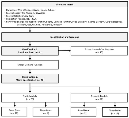
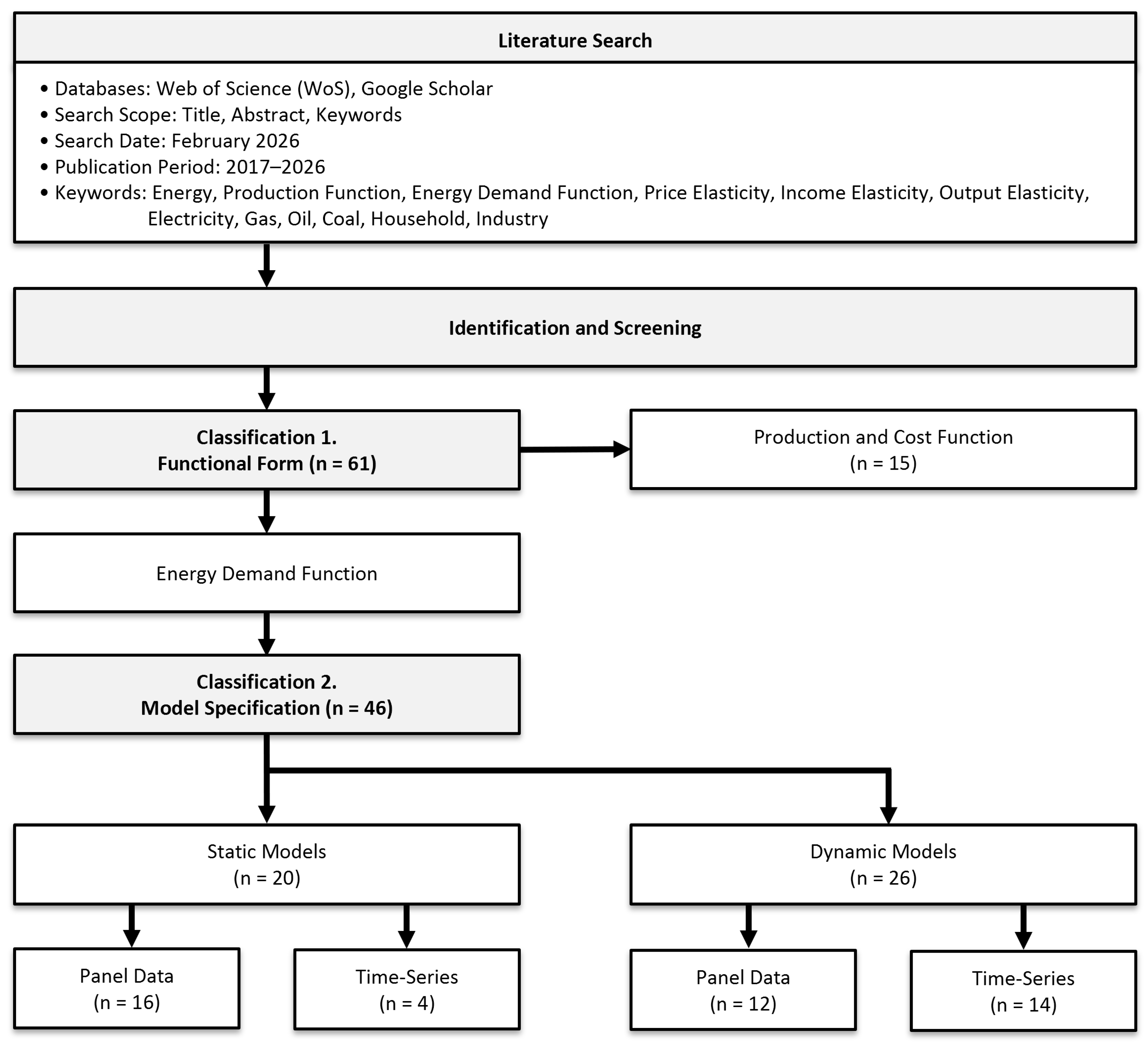

Disclaimer/Publisher’s Note: The statements, opinions and data contained in all publications are solely those of the individual author(s) and contributor(s) and not of MDPI and/or the editor(s). MDPI and/or the editor(s) disclaim responsibility for any injury to people or property resulting from any ideas, methods, instructions or products referred to in the content. |
© 2026 by the authors. Licensee MDPI, Basel, Switzerland. This article is an open access article distributed under the terms and conditions of the Creative Commons Attribution (CC BY) license.