Adaptive Global Control with jDE and Grid Search for Energy-Saving Optimization of Data Center Central Air Conditioning Systems

Abstract

This study develops a simulation-based plant-level supervisory optimization framework for a Nanjing data center chilled-water plant by combining TRNSYS operating scenarios, fitted component-level surrogate models, and self-adaptive differential evolution (jDE). In the exported representative-case optimization, the decision variables are the cooling-tower approach temperature difference, cooling-water temperature difference, chilled-water temperature difference, and the common cooling-tower fan frequency, while chilled-water supply temperature is carried through as the matched scenario input and examined separately through a 14–18 °C sensitivity sweep. The system comprises three chillers, three cooling towers, three chilled-water pumps, and three cooling-water pumps. The retrained chiller support covers nominal chilled-water supply settings of 14, 15, 16, 17, and 18 °C with hourly sample counts of 8759, 8759, 8760, 8759, and 8759, respectively, yielding an in-support fitted range of approximately 14.0–18.0 °C. For 48 representative operating cases selected from four seasonal days, the optimized operation reduces total power by 17.24–33.55% (mean 27.34%) and increases system COP by 20.78–50.42% (mean 38.12%), relative to matched baseline values at the same timestamps. After enforcing the fitted chiller cooling-water support floor, the largest average relative gain appears in summer rather than winter. Component-level analysis shows that the corrected savings are generated mainly by pump and cooling-tower relief, with chiller-power changes remaining secondary and season dependent. All reported results are derived from matched simulation-based baseline and optimized evaluations rather than field measurements, and all 48 representative cases remain within the fitted chiller support, with optimized cooling-water supply temperatures ranging from 20.05 to 27.75 °C.

1. Introduction

Driven by the continued expansion of cloud computing, big data, artificial intelligence, and 5G services, data centers have become an indispensable infrastructure of the digital economy, and their rising electricity demand has emerged as a major energy and environmental concern. Global data center electricity consumption was estimated at 200–250 TWh in 2020, equivalent to about 1–1.3% of total electricity use, and may rise to 500–600 TWh by 2030 [1,2]. In China, rapid growth in high-performance computing and cloud services has accelerated data center deployment, while national efficiency policies continue to tighten power usage effectiveness targets for large facilities toward 1.25 by 2025 [3,4]. Under high server density, time-varying IT load, and changing wet-bulb conditions, improving cooling-system efficiency is, therefore, essential for reducing electricity use, supporting low-carbon development, and maintaining reliable operation [5,6]. Because cooling demand in a data center cannot simply be curtailed without compromising thermal safety, much of the practical efficiency improvement must come from better coordination of the cooling plant itself.

Within such facilities, the central air-conditioning system commonly accounts for 30–50% of total electricity consumption and is, therefore, a primary target for PUE reduction [7,8]. Prior studies have shown that optimized supervisory control can reduce chiller power from about 250 kW to 210 kW and pump power from 16–48 kW to approximately 16 kW [9,10]. Raising chilled-water supply temperature can also reduce annual energy use, with reported annual savings of 14.8% and marked decreases in chiller and chilled-water pump demand [11,12,13]. Chen et al. [14] further showed that larger chilled-water temperature differences influence both energy-saving potential and equipment sizing. Coordinated adjustment of cooling-tower fan frequency and pump flow has likewise been reported to reduce energy use by about 10% under high load while maintaining cold-aisle temperature stability [15,16]. These findings confirm the considerable potential of central air-conditioning optimization, but they also show that local savings on one component cannot be taken as evidence of minimum whole-system power because chillers, pumps, and cooling towers remain strongly coupled [17,18,19,20].

Traditional fixed-setpoint or rule-based strategies remain limited when load and weather conditions vary rapidly [18,19]. In a strongly coupled chilled-water plant, an operating adjustment that reduces the demand of one component can simultaneously increase the burden of the others and therefore fail to minimize total system power [9,20]. At the same time, high-fidelity nonlinear models are often too computationally expensive for repeated supervisory optimization and rapid updating [12,21,22,23]. The modeling of cooling-tower approach temperature is especially challenging because fan frequency, water flow, and wet-bulb-driven heat rejection must be represented simultaneously [7,18,24].

The practical challenge is therefore twofold: the optimization variables must remain physically meaningful and closely tied to plant operation, yet the resulting model must be light enough for a repeated search across many operating cases. This tension between physical coupling and computational tractability motivates the present combination of scenario-based simulation and surrogate modeling.

In recent years, model-based, learning-based, and metaheuristic strategies have been increasingly applied to data center and chiller-plant optimization [25,26,27,28,29,30]. MPC-oriented studies by Trautman et al. [9], Lazic et al. [5], and Ogura et al. [17] showed the benefit of coordinated chiller and cooling-tower adjustment under varying load and ambient conditions. Reinforcement-learning and physics-informed approaches were subsequently reported for HVAC and chiller-plant optimization, including deep reinforcement learning [27], physics-informed neural-network control [28], and reinforcement-learning/differential-evolution hybrids for strongly coupled operating conditions [11]. Additional work based on genetic algorithms, particle swarm optimization, artificial immune systems, and related data-driven optimizers likewise reported meaningful savings for coupled cooling plants [15,24,26,29,30]. Even so, three blind spots recur across the literature: reported percentage savings are often emphasized more strongly than model fidelity, computational burden, and constraint satisfaction; the respective roles of scenario generation, surrogate modeling, and supervisory optimization are not always distinguished clearly; and component-level power migration is seldom analyzed in enough detail to reveal whether an apparent auxiliary saving is being offset elsewhere in the plant. Related thermodynamic and reduced-order studies on vapor-compression systems further show that compact models can preserve the dominant physical response while lowering computational cost, which provides a stronger physical basis for the use of surrogate models in plant-level optimization [31,32,33].

Against this backdrop, the present paper returns to the original Nanjing data center case comprising three chillers, three cooling towers, three chilled-water pumps, and three cooling-water pumps, and recasts it as a plant-level optimization benchmark with a clearer evidential boundary. The purpose is not merely to obtain a lower objective value, but to keep the optimization architecture transparent enough to show how scenario generation, surrogate modeling, and supervisory search each contribute to the final result. jDE is adopted as the primary solver because the search space is continuous, nonlinear, and strongly coupled, with explicit operating bounds and changing active-device combinations; compared with fixed-parameter GA or PSO schemes, it requires less case-by-case retuning when seasonal conditions shift. Grid search is retained only as a transparent benchmark reference. The revised analysis, therefore, interprets representative-day performance together with model-fit accuracy, computational burden, chilled-water supply temperature sensitivity, and configuration-based constraint margins, so that the seasonal results can be read as whole-system evidence under clearly stated simulation assumptions.

Within this clarified scope, the contribution of the study lies less in proposing an abstract new optimizer than in turning the original case into a more transparent supervisory benchmark. The manuscript preserves the explicit multi-device Nanjing plant configuration and reconstructs it through component-wise surrogate fitting rather than an aggregate black-box formulation; it extends the chiller-model support with the supplied 14/15/17/18 °C cases so that the 14–18 °C chilled-water supply discussion rests on a broader fitted basis; and it evaluates the resulting savings together with seasonal operating profiles, solver-runtime behavior, sensitivity analysis, and configuration-level constraint margins. Taken together, these steps provide a firmer basis for judging not only the magnitude of the simulated energy benefit, but also the limits within which that benefit can presently be interpreted.

2. Methodology

2.1. Nanjing Data Center Water System TRNSYS Simulation Platform

2.1.1. Contextual Overview and Equipment Specifications

The case study is a Nanjing data center cooling scenario represented in TRNSYS 18 rather than a fully instrumented field deployment. The simulation platform was developed in TRNSYS 18. The plant includes three chillers, three cooling towers, three cooling-water pumps, and three chilled-water pumps and serves a 3000 m² facility under a schedule-driven internal heat load of 4600 kW. Weather boundary conditions are supplied by a Nanjing weather dataset. Accordingly, all baseline and optimized values reported in the following sections are derived from matched simulation cases at selected timestamps rather than from field measurements.

The case represents a continuously cooled, high-load data center environment. The three-chiller, three-tower, and matched pump-group arrangement defines the multi-device coordination problem addressed here because any operating adjustment that benefits one component immediately alters the feasible operating region of the others through shared thermal, hydraulic, and heat-rejection relationships. For this reason, the case definition and boundary assumptions are summarized in Table 1, and the season-by-season representative-day analysis is retained rather than replacing the plant with a purely abstract optimization problem.

Table 1. Case definition and boundary assumptions used in this study.

Item	Value
Scenario type	Nanjing data center chilled-water plant scenario in TRNSYS
Building area	3000 m2
Geometry	60 m × 50 m × 4 m
Cooling load assumption	4600 kW schedule-driven internal IT heat load
Load source	Assumed annual schedule in TRNSYS Type56 rather than measured plant data
Equipment layout	Three chillers, three cooling towers, three cooling-water pumps, three chilled-water pumps
Weather input	Nanjing weather file via TRNSYS Type109
Time horizon for training	8760 h synthetic operating dataset
Main reproduced benchmark	12 sampled points on each of 21 March, 31 July, 15 October, 31 December (48 cases total)
Validation status	No measured calibration or TRNSYS-to-field validation available in this study

2.1.2. TRNSYS Module Assembly

TRNSYS generates 8760 h of annual operating data, and the optimization step relies on separate surrogate models fitted from those outputs. The primary fitting dataset is the annual TRNSYS-derived training dataset. The chiller-power models are further retrained with an augmented dataset that combines the original annual scenario data and the newly supplied 14/15/17/18 °C hourly chilled-water supply cases, whereas the pump and cooling tower surrogates remain trained on the original annual scenario dataset. Chiller power is fitted with an eight-parameter nonlinear curve-fit formulation using cooling load, cooling-water supply temperature, and chilled-water supply temperature. Cooling-water pumps and chilled-water pumps are fitted with second-order polynomial models, while cooling-tower fan power now uses an adaptive polynomial surrogate with degree 2–4 selected from fit quality. Cooling-tower heat rejection is fitted with a second-order polynomial-interaction surrogate using water flow, fan frequency, cooling-water return temperature, and outdoor wet-bulb temperature.

In this formulation, TRNSYS provides the operating scenarios, equipment interactions, and baseline reference trajectories, whereas the fitted surrogates provide the fast algebraic layer required for repeated optimization across the representative operating cases.

The analytical structure, therefore, contains three linked layers: annual scenario generation in TRNSYS, component-wise surrogate identification from those scenarios, and constrained optimization with matched-case verification at representative timestamps. This layered formulation is important because it preserves the physical meaning of the original case while avoiding the prohibitive computational cost of embedding the full simulation within every optimizer evaluation.

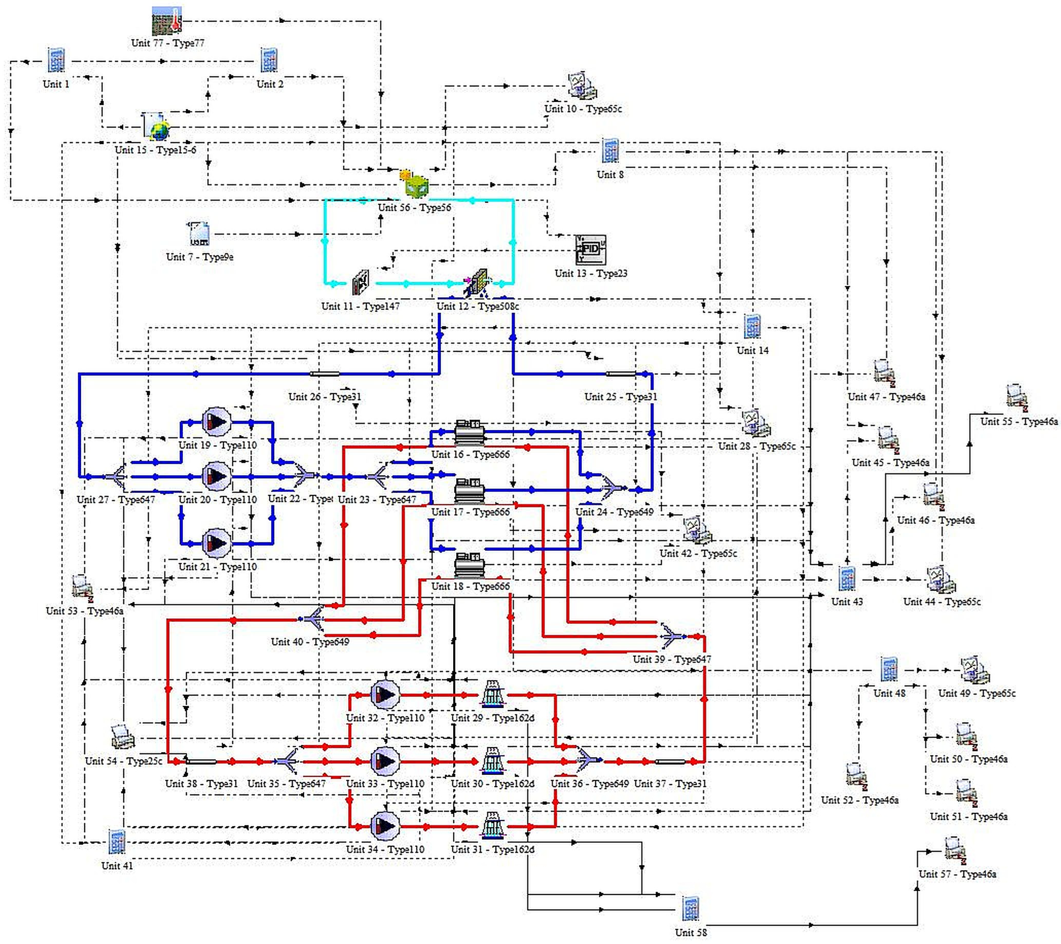
At the module level, the load side uses Type56 for the multi-zone data center space, Type109 for the Nanjing weather boundary, Type147 and Type508 for the return-fan and air-handling-unit path, and Type23 for the PID-based air-side regulation. On the water side, the platform uses Type666 chillers, Type110 variable-frequency pumps, Type162 cooling towers, and Type647/Type649 together with Type31 piping to close the chilled-water and cooling-water loops.

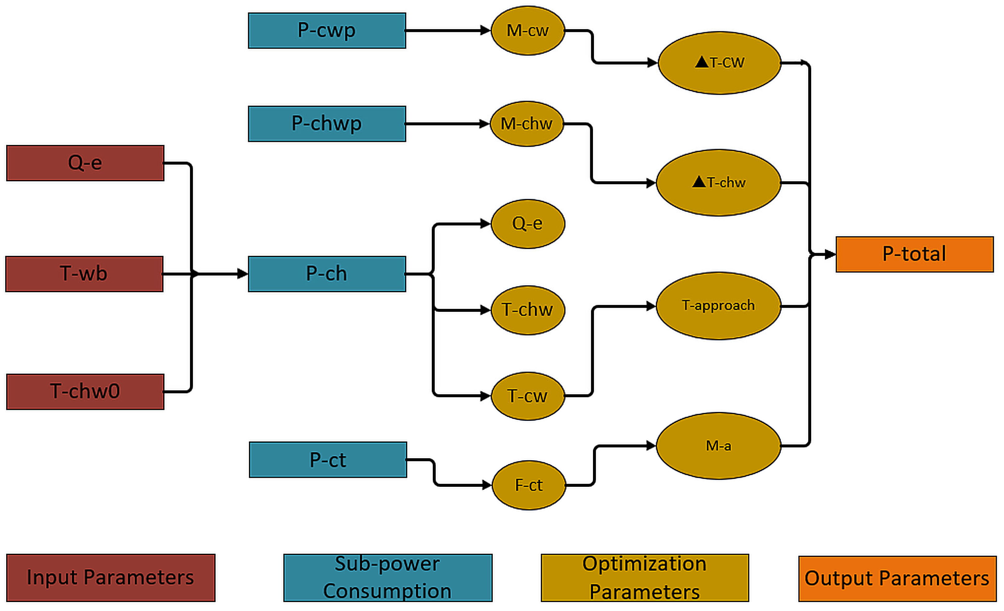
The load side represents the building and air-side scenario, while the water-side system couples chillers, pumps, cooling towers, mixing devices, and piping elements into one closed plant. The baseline operating logic uses chilled-water supply temperature, cooling-water and chilled-water temperature differences, and tower-side heat rejection as the main supervisory levers. In the exported representative-case optimization, the matched chilled-water supply temperature from each TRNSYS scenario is passed through as a fixed case input, whereas the optimization acts on approach temperature difference, cooling-water temperature difference, chilled-water temperature difference, and a common tower frequency.

Figure 1 and Figure 2 summarize the TRNSYS system structure and the dependency among the principal control variables. These schematics define the physical arrangement of the case study and the relationships among the optimized variables discussed in the following sections.

Figure 1. TRNSYS system-platform schematic of the Nanjing chilled-water plant, identifying the coupled chiller, pump, and cooling-tower subsystems represented in the scenario model. Different colored paths distinguish the main chilled-water, cooling-water, and air-side/control connections.

Figure 2. Parameter-dependency schematic of the baseline control logic, showing how the principal supervisory variables propagate through the coupled plant. The colored boxes denote the input-parameter, sub-power-consumption, optimization-parameter, and output-parameter layers.

The coefficients in Equations (1)–(6) are obtained from these regressions. Appendix A summarizes the corresponding fitting method, training data, and valid input ranges for each component model. The result tables also distinguish baseline simulation outputs from optimized rerun outputs and report the pump-flow and tower-frequency bounds used in the feasibility analysis.

2.2. Simulation Data Generation

The annual TRNSYS simulation is first run at the native scenario resolution and then condensed into representative operating points for comparative analysis. Within this baseline operating context, the chilled-water supply temperature is initialized at 16 °C, tower control is linked to the outdoor wet-bulb temperature, and pump operation follows temperature-difference logic with equipment-level minimum frequency limits. Retaining these settings makes it possible to evaluate the influence of the 16 °C baseline chilled-water supply setting through a dedicated sensitivity analysis without disconnecting the comparison from the original plant scenario.

The TRNSYS scenario is run across 8760 hourly operating points, and the representative seasonal days used in this study are 21 March, 31 July, 15 October, and 31 December. Baseline and optimized evaluations are extracted at these representative timestamps so that the numerical claims remain tied to one consistent case set. In the exported main case chain, chilled-water supply temperature remains the matched scenario input near 16 °C, whereas the 14–18 °C chilled-water supply sweep is reported separately as a one-factor sensitivity study built on the retrained chiller support.

Each representative day is sampled through twelve characteristic operating points spanning the daily load trajectory from 02:00 to 24:00. This sampling scheme preserves the seasonal before/after comparison while maintaining a consistent connection between the annual TRNSYS simulations used for model fitting and the representative operating points used for quantitative comparison.

The representative days are not introduced merely as a convenient subset of hours. Instead, they are used to retain the original engineering narrative of spring, summer, autumn, and winter operation, allowing the manuscript to compare how the same optimization structure behaves under moderate, severe, transitional, and favorable condenser-side conditions.

A separate 14–18 °C chilled-water supply sensitivity study is presented rather than merged into the main performance comparison. This avoids contaminating the core baseline versus optimized statistics with a one-factor sensitivity sweep, while still allowing the study to assess whether the commonly used 16 °C initial setting is conservative, aggressive, or near the favorable end of the currently fitted operating range.

The plant is also staged according to load demand, with additional chillers enabled as the active set approaches rated capacity, and the associated pumps and cooling towers are matched to the running chiller count. This operating sequence defines the feasible equipment combinations from which the evaluated case set and surrogate training samples are drawn. The optimization problem, therefore, acts on an existing staged plant rather than on an unconstrained unit-commitment formulation.

2.3. System Modeling and Holistic Optimization

2.3.1. System Energy Consumption Model Construction

The optimization objective remains single-objective total-power minimization. Thermal comfort, cooling-duty security, and equipment wear are not introduced as parallel objectives in this study. Instead, IT-side heat removal and plant heat-balance satisfaction are enforced through the load-flow-heat-balance equations and the configured operating bounds; therefore, any candidate that cannot satisfy the cooling-duty constraints is rejected as infeasible. Equipment-wear implications are then examined through margin analysis and adjacent-control-movement statistics. This formulation preserves a clear correspondence between the reported saving and the model that is actually solved, while avoiding unsupported claims of a multi-objective capability.

At the modeling level, total plant power is decomposed into chiller, cooling-water pump, chilled-water pump, and cooling-tower fan power rather than treated as one monolithic black-box output. This mirrors the physical composition of the original plant. Because each component has its own fitted surrogate, this study can report device-specific MAPE, RMSE, R², input ranges, coefficient sets, and post-optimization power migration, instead of forcing all uncertainty and all savings into a single opaque aggregate indicator.

All major bounds are taken from the actual operational configuration instead of hard-coded values. Pump flow limits, cooling-tower frequency limits, and temperature bounds are reported together with the optimization results so that any feasibility issue can be interpreted against the true configured thresholds. For cooling-water supply temperature, the effective lower bound is the larger of the configured physical floor and the fitted chiller-support floor (19.9274 °C), which makes the effective lower approach bound scenario dependent under low wet-bulb conditions. No standalone hard efficiency threshold is imposed in the present formulation.

The component-power models and coupling relationships are expressed in Equations (1)–(6).

$${\mathrm{P}}_{\mathrm{total}}=\sum {\mathrm{P}}_{\mathrm{ch}}+\sum {\mathrm{P}}_{\mathrm{chwp}}+\sum {\mathrm{P}}_{\mathrm{cwp}}+\sum {\mathrm{P}}_{\mathrm{ct}}$$

(1)

$$\begin{array}{c}{\mathrm{P}}_{\mathrm{ch}}={ \mathrm{a}}_0+{ \mathrm{a}}_1{\mathrm{Q}}_{\mathrm{e}}+{ \mathrm{a}}_2{\mathrm{t}}_{\mathrm{chw}}+{ \mathrm{a}}_3{\mathrm{t}}_{\mathrm{cw}}+{ \mathrm{a}}_4{{\mathrm{Q}}_{\mathrm{e}}}^2+{ \mathrm{a}}_5{\mathrm{Q}}_{\mathrm{e}}{\mathrm{t}}_{\mathrm{chw}}\\ +{\mathrm{a}}_6{\mathrm{Q}}_{\mathrm{e}}{\mathrm{t}}_{\mathrm{cw}}+{\mathrm{a}}_7{\mathrm{t}}_{\mathrm{cw}}{\mathrm{t}}_{\mathrm{chw}}\end{array}$$

(2)

$${\mathrm{P}}_{\mathrm{chwp}}={\mathrm{a}}_0+{\mathrm{a}}_1\cdot {\mathrm{m}}_{\mathrm{chw}}+{\mathrm{a}}_2\cdot {\mathrm{m}}_{\mathrm{chw}}^2$$

(3)

$${\mathrm{P}}_{\mathrm{cwp}}={\mathrm{a}}_0+{\mathrm{a}}_1\cdot {\mathrm{m}}_{\mathrm{cw}}+{\mathrm{a}}_2\cdot {\mathrm{m}}_{\mathrm{cw}}^2$$

(4)

$${\mathrm{P}}_{\mathrm{ct}}={ \mathrm{a}}_0+{\mathrm{a}}_1\cdot {\mathrm{f}}_{\mathrm{ct}}+{ \mathrm{a}}_2\cdot {\mathrm{f}}_{\mathrm{ct}}^2$$

(5)

$${\mathrm{Q}}_{\mathrm{ct}}={\displaystyle \frac{\mathrm{a}\cdot {\mathrm{m}}_{\mathrm{cw}}^{\mathrm{b}}}{1+\mathrm{c}\cdot {\left(\frac{{\mathrm{m}}_{\mathrm{cw}}}{{\mathrm{m}}_{\mathrm{a}}}\right)}^{\mathrm{b}}}}\cdot ({\mathrm{t}}_{\mathrm{cw}} - {\mathrm{t}}_{\mathrm{wb}})$$

(6)

$${\mathrm{m}}_{\mathrm{chw}}={\displaystyle \frac{{\mathrm{Q}}_{\mathrm{e}}}{\mathsf{\rho }\cdot {\mathrm{c}}_{\mathrm{p}}\cdot \mathsf{\Delta }{\mathrm{t}}_{\mathrm{chw}}}}$$

(7)

$${\mathrm{m}}_{\mathrm{cw}}={\displaystyle \frac{{\mathrm{Q}}_{\mathrm{ct}}}{\mathsf{\rho }\cdot {\mathrm{c}}_{\mathrm{p}}\cdot \mathsf{\Delta }{\mathrm{t}}_{\mathrm{cw}}}}$$

(8)

$${\mathrm{Q}}_{\mathrm{e}}+{ \mathrm{P}}_{\mathrm{chiller}}={\mathrm{Q}}_{\mathrm{ct}}$$

(9)

For readability, the principal symbols used in Equations (1)–(6) are defined in the Nomenclature and follow standard mathematical notation with subscripts. The objective term represents total plant power; the component terms represent chiller, cooling-water pump, chilled-water pump, and cooling-tower fan power; the load term represents cooling demand; the flow terms represent chilled-water and cooling-water flow rates; the fan frequency term represents cooling-tower fan speed; the heat-rejection term represents cooling-tower heat rejection; the temperature terms represent the inlet temperature and the chilled-water/cooling-water temperature differences; and the remaining coefficient terms are fitted regression parameters.

Equations (1)–(6) define the total-power objective and the component models for chillers, cooling-water pumps, chilled-water pumps, cooling-tower fan power, and cooling-tower heat rejection. Their numerical coefficients are obtained from the fitted surrogate models and are listed in Appendix A.

Within this formulation, the system objective is expressed as total plant power, and each component term is evaluated through the corresponding fitted surrogate under the prescribed operating bounds. Table 2 lists the configured or derived bounds; in the representative-case optimization, T_chw,s is passed through from the matched scenario case, whereas the 14–18 °C interval is assessed separately in the sensitivity study.

Table 2. Operational bounds and device limits used in the optimization.

Variable	Lower Bound	Upper Bound
Matched chilled-water supply input in representative cases	scenario derived	scenario derived
Chilled-water supply temperature (sensitivity sweep only)	14.0	18.0
Approach temperature difference	max(2.0, Tcw,s,min − Twb)	case dependent
Cooling-water temperature difference	4.0	8.0
Chilled-water temperature difference	4.0	8.0
Cooling-tower fan frequency	10	50
Per cooling-water pump flow	133.07	332.68
Per chilled-water pump flow	117.10	292.75
Cooling-water supply temperature	max(10.0, 19.9274)	dynamic/derived
Cooling-water return temperature	dynamic/derived	40.0
Chilled-water return temperature	18.0	26.0

2.3.2. Equipment Coupling Characteristics

The chiller, chilled-water pumps, cooling-water pumps, and cooling towers form a tightly coupled water-side system. Reducing one component’s power does not automatically imply whole-system improvement because cooling-water flow, chilled-water flow, fan frequency, and heat-rejection capability interact through shared thermal and hydraulic constraints. This is why the study examines component-migration tables and explicit constraint margins rather than evaluating single devices in isolation.

The coupling is both spatial and sequential. In the representative-case optimization, changes in cooling-water temperature difference, chilled-water temperature difference, and tower-side operation reshape pump demand, condenser-side heat rejection, and chilled-water return temperature. In the separate chilled-water supply temperature sensitivity study, varying T_chw,s further changes chiller lift and transport demand. Sequentially, adjacent representative cases belong to one daily operating trajectory.

2.3.3. Global Optimization Problem

The optimization problem is formulated as a whole-system operating-point search rather than as a single-device tuning exercise. The implemented objective is to minimize the total plant power predicted by the surrogate set, namely the combined chiller, cooling-water pump, chilled-water pump, and cooling-tower fan power. For each matched representative case, the decision variables are cooling-tower approach temperature difference, cooling-water temperature difference, chilled-water temperature difference, and the common cooling-tower fan frequency, while chilled-water supply temperature enters as the matched scenario input T_chw,s0, and is varied separately only in the dedicated 14–18 °C sensitivity study.

These variables span the main supervisory degrees of freedom used in the present exported case chain. The approach variable fixes cooling-water supply temperature through the T_cw,s = Twb + approach, the two temperature-difference variables regulate transport intensity and return-side conditions on the cooling-water and chilled-water loops, and the common tower-frequency variable governs auxiliary heat-rejection effort.

These variables are supervisory control variables only. The optimizer does not change hardware configuration, equipment sizing, or plant topology. The reported reductions in total power and increases in COP should, therefore, be interpreted strictly as operational gains under fixed installed equipment. This clarification matters when comparing the present results with studies that report savings from structural retrofits, free-cooling hardware additions, or different chiller-plant architectures.

The feasible region is defined by the actual operational configuration rather than by idealized assumptions. Temperature bounds, per-pump flow bounds, and cooling-tower frequency bounds are all applied consistently to the optimized cases. Heat rejection and cooling-duty satisfaction are checked through a tolerance-based heat-balance constraint; therefore, any candidate that cannot remove the required load within the configured residual band is discarded as infeasible. Feasibility, therefore, means staying inside the configured residual band rather than forcing a strictly positive margin at every reproduced timestamp. In practice, the representative-case batch, therefore, enforces T_cw,s ≥ 19.9274 °C whenever the fitted chiller support is tighter than the configured physical minimum.

The optimization problem is, therefore, minimized subject to the previously defined physical and mass-balance constraints in Equations (7)–(9), together with the configured temperature, flow, tower frequency, and tolerance-based heat-balance feasibility limits.

$$\min {\mathrm{P}}_{\mathrm{total}}=\sum {\mathrm{P}}_{\mathrm{ch}}+\sum {\mathrm{P}}_{\mathrm{chwp}}+\sum {\mathrm{P}}_{\mathrm{cwp}}+\sum {\mathrm{P}}_{\mathrm{ct}}$$

(10)

In other words, the constraint block serves as the hard cooling-safety screen used in case evaluation: load balance, loop temperature-difference relationships, configured equipment bounds, and tolerance-based heat rejection must all remain satisfied for a case to be counted as feasible.

2.3.4. Optimization Algorithms

A comparative assessment of jDE, grid search, and local refinement is carried out for the representative-case set. Self-adaptive differential evolution (jDE) is used as the primary global optimizer because it handles the continuous, nonlinear, and strongly coupled search space without requiring repeated discretization redesign across operating points. Grid search is used as a transparent benchmark check under the selected discretization, while a fast local multi-start solver is included as an auxiliary computational reference.

Accordingly, the numerical study is framed as an offline methodological comparison on representative operating cases rather than as a deployment study of an online MPC controller. TRNSYS provides the scenario data, surrogate models are fitted from those data, and the alternative optimizers are evaluated on a common case set. Runtime and feasibility results are, therefore, reported to characterize methodological suitability for this study.

Within this comparison, grid search serves as a transparent benchmark rather than as a universal fine-tuning stage for every case. Its role is to show whether the jDE solution is consistent with an interpretable lattice-based search under the selected discretization. The added fast local solver serves as a computationally inexpensive acceleration reference, but it is not treated as a general replacement for the global search when the feasible region becomes strongly coupled or nonconvex.

3. Results and Discussion

3.1. Seasonal Typical Day Performance

For 48 representative operating cases selected from four seasonal days, the mean total power saving reaches 27.93% on 21 March, 29.30% on 31 July, 27.04% on 15 October, and 25.10% on 31 December. The corresponding mean COP improvements are 39.34%, 41.72%, 37.50%, and 33.90%, respectively.

A different seasonal ordering emerges once the fitted chiller cooling-water support floor is enforced. Summer now shows the largest average relative gain because its baseline remains the most condenser-limited, with a mean baseline COP of only 4.9731 before optimization. Winter still reaches a high optimized COP of 8.0800, but it records the smallest relative improvement because its baseline efficiency is already comparatively strong at 6.0503.

On 21 March, the plant operates under comparatively moderate load and wet-bulb conditions, and optimization delivers a mean power saving of 27.93% with a day-level range of 19.41–32.93%. The corresponding COP improvement spans 24.09–49.12%.

On 31 July, the plant faces the harshest condenser-side condition among the four representative days. This is reflected in the lowest baseline COP of 4.9731 and in the highest mean power saving of 29.30%. Even under the most severe tower-side burden, the representative cases still achieve a day-level power-saving range of 23.41–33.55% and a COP-improvement range of 30.55–50.42%.

The transitional 15 October case lies close to the spring pattern, with a mean power saving of 27.04% and a mean COP improvement of 37.50%. By contrast, 31 December shows the smallest relative improvement envelope after the support-aware correction, with a mean power saving of 25.10% and a COP improvement range of 20.78–42.15%.

The expanded seasonal summary is listed in Supplementary Table S1, while the main text focuses on the physical mechanisms revealed by the representative cases and their corresponding hourly figures.

3.1.1. 21 March Representative-Day Profile

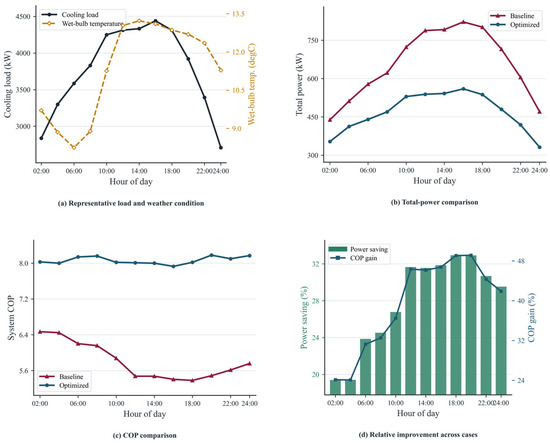
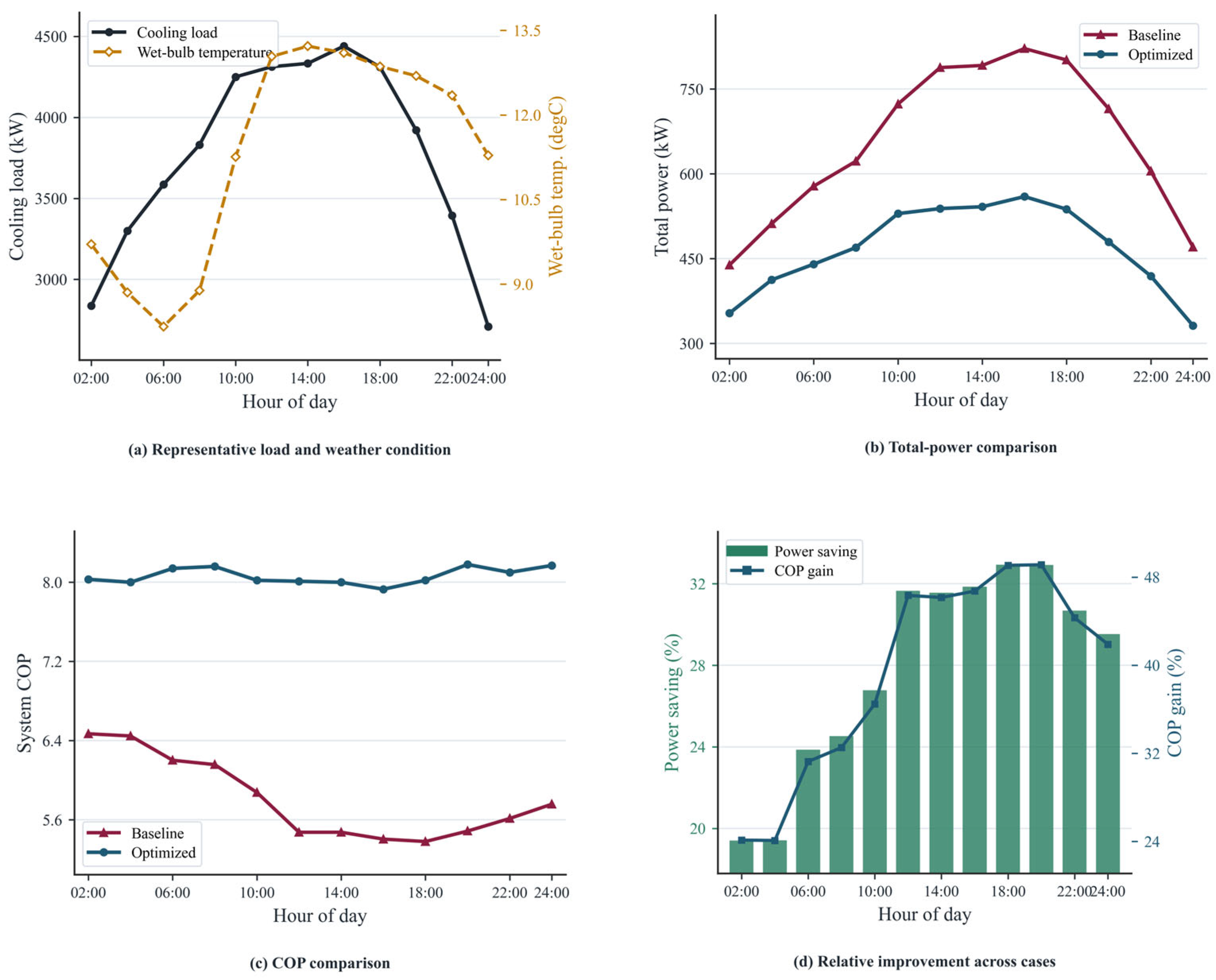
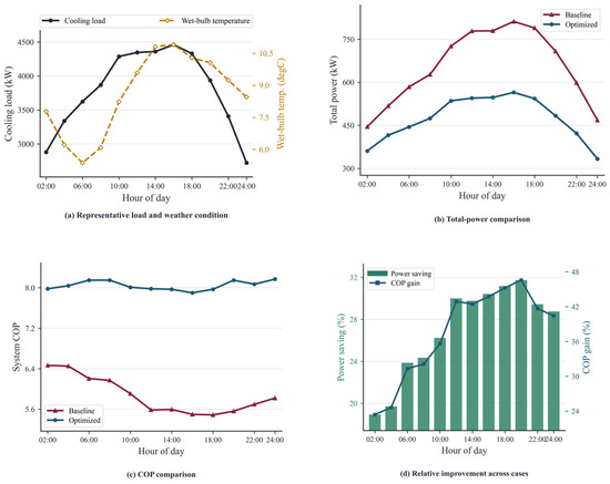
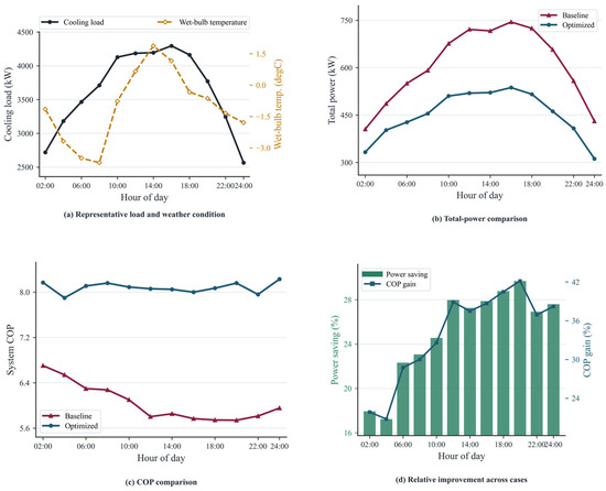
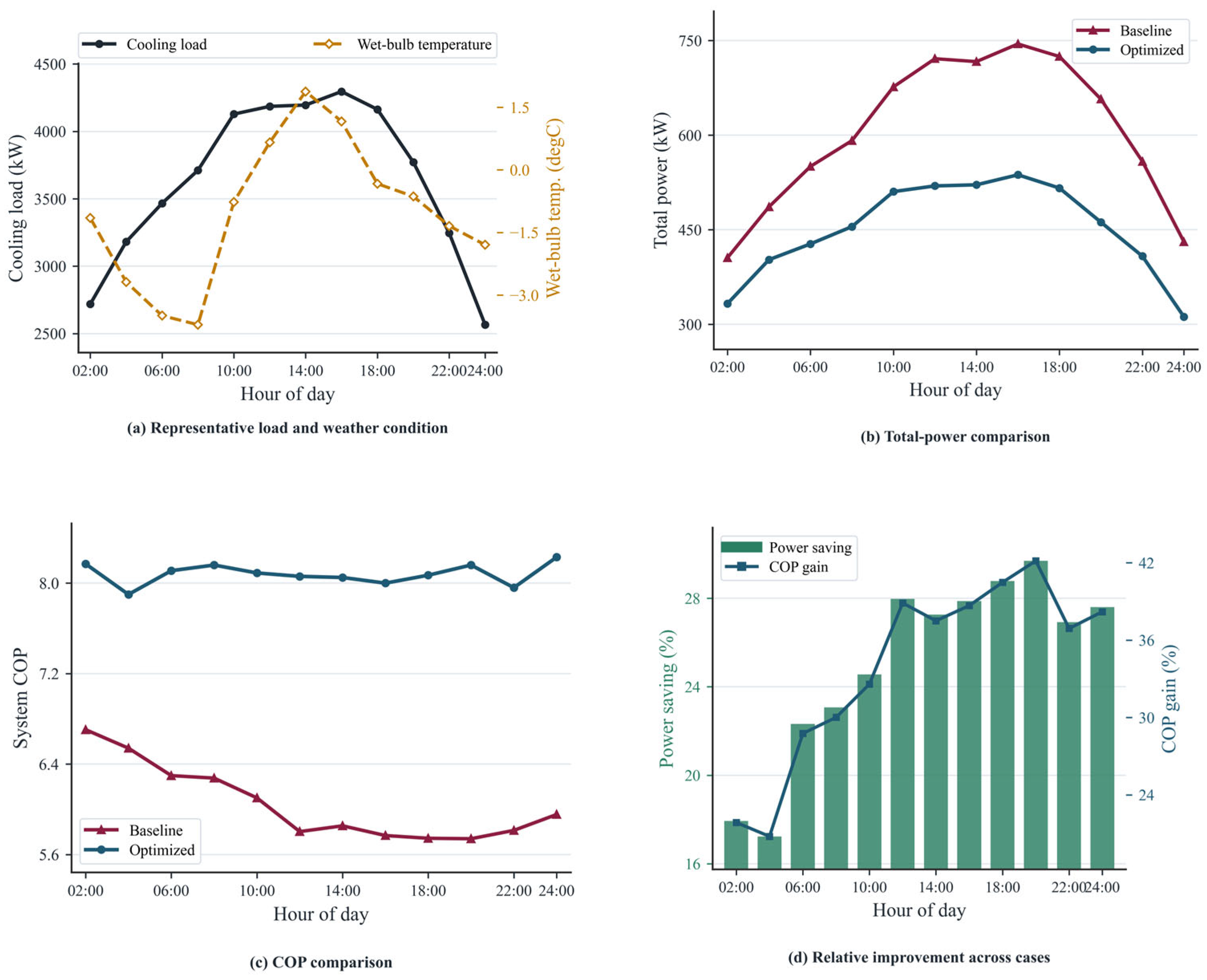
On 21 March, the cooling load varies from 2709.08 to 4439.80 kW while the outdoor wet-bulb temperature ranges from 8.25 to 13.22 °C. The baseline mean total power declines from 655.53 to 467.75 kW after optimization, while the mean COP rises from 5.8115 to 8.0633. The optimized absolute cooling-water supply temperature settles near 20.175 °C.

The spring benefit is distributed across the day. The cooling load crest reaches 4439.80 kW at 16:00, and the highest wet-bulb temperature reaches 13.22 °C at 14:00. A maximum power reduction of 32.93% is recorded at 18:00, while the maximum COP gain of 49.12% appears at 20:00; even the weakest hour at 02:00 still preserves 19.41% saving.

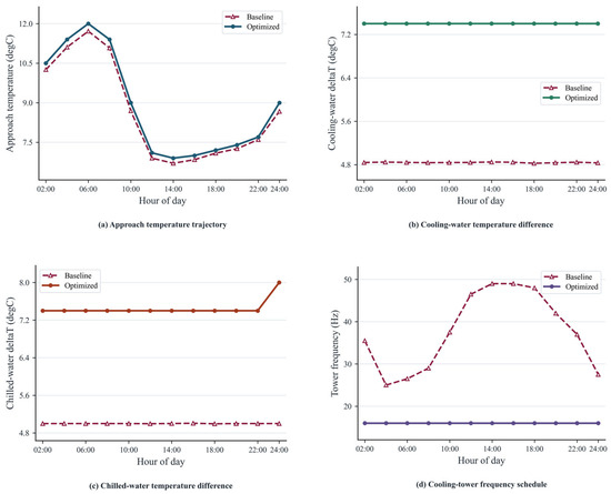
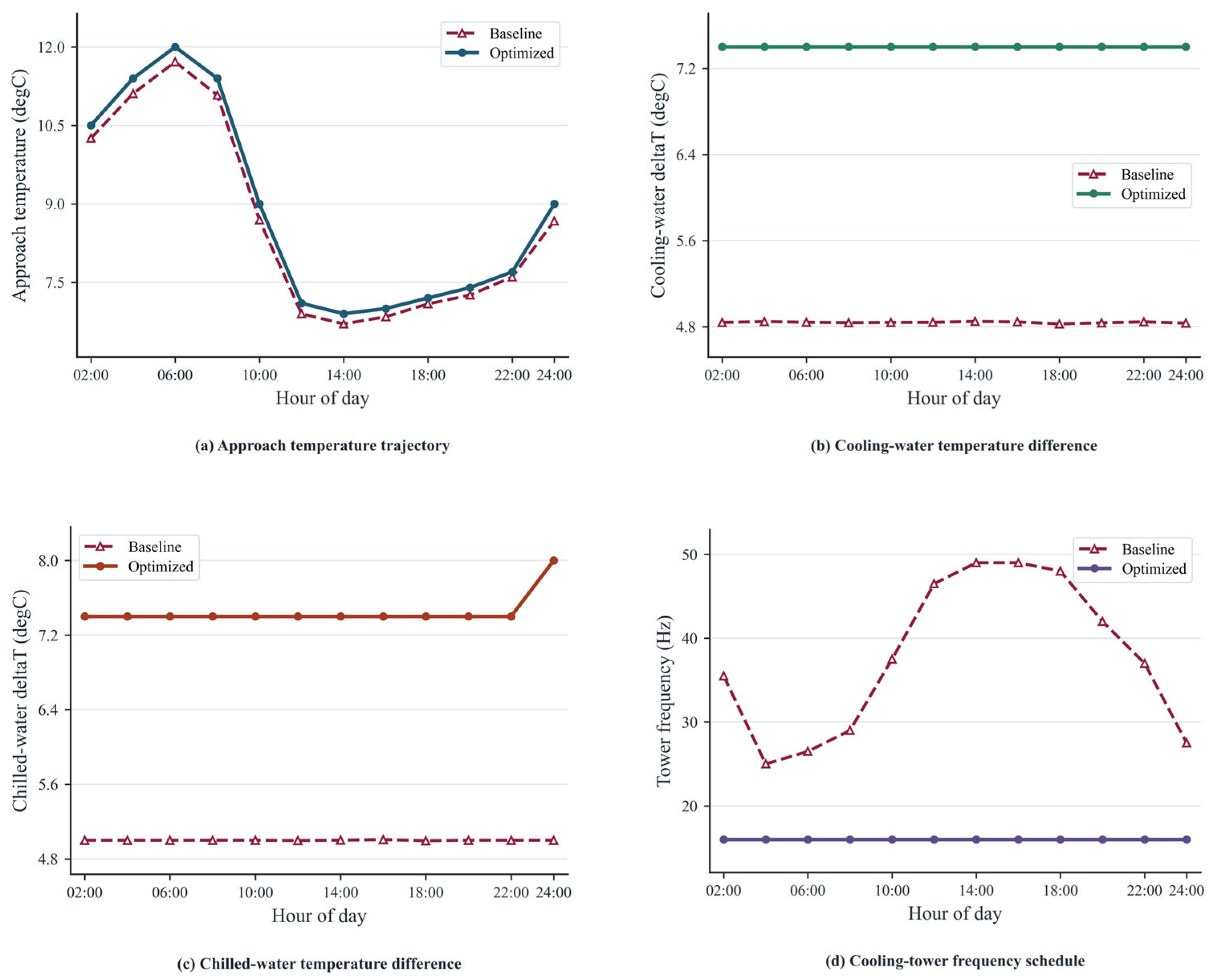
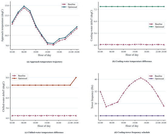
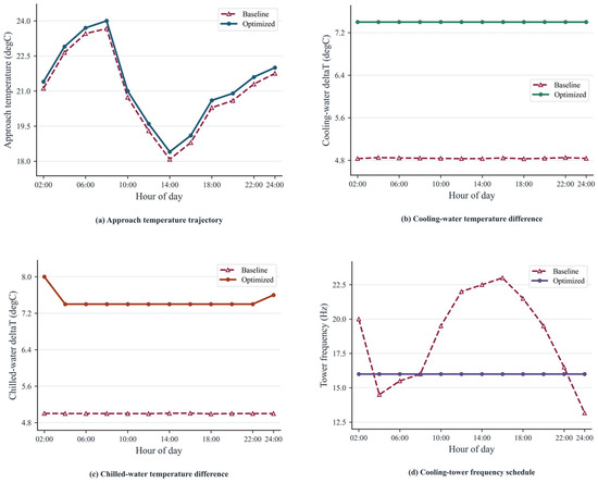
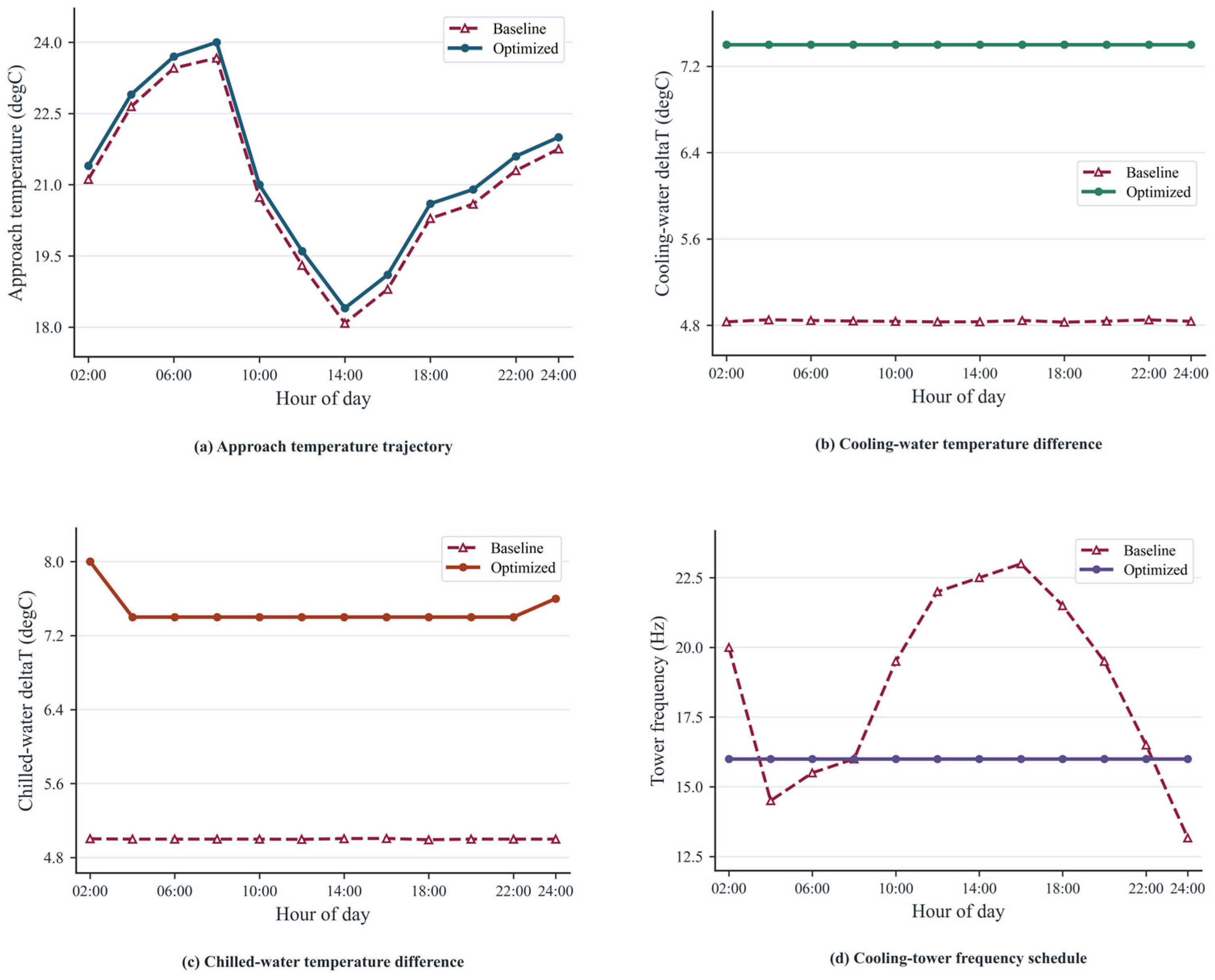
Figure 3 and Figure 4 show that the optimized spring schedule lowers auxiliary demand while holding the absolute cooling-water supply temperature close to the fitted support floor. The mean approach temperature changes only slightly from 8.66 to 8.88 °C, tower frequency drops from 37.71 to 16.00 Hz, cooling-water flow from 737.71 to 481.12 m³/h, and chilled-water flow from 649.18 to 435.91 m³/h.

Figure 3. Hourly operating-parameter trajectories for 21 March. After the cooling-water support correction, the optimized spring profile is characterized mainly by lower tower frequency and lower loop flow rates, while the absolute cooling-water supply temperature remains near the fitted floor.

Figure 4. Hourly total-power and COP comparison for 21 March. The optimized spring profile preserves positive whole-system benefit throughout the day without relying on unrealistic condenser overcooling.

Supplementary Table S2 provides the compact day summary corresponding to Figure 3 and Figure 4.

3.1.2. 31 July Representative-Day Profile

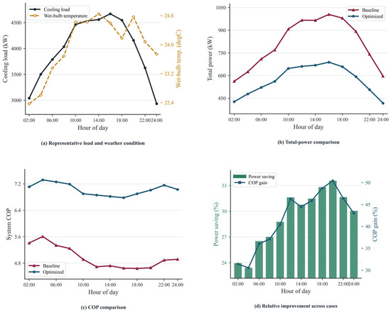
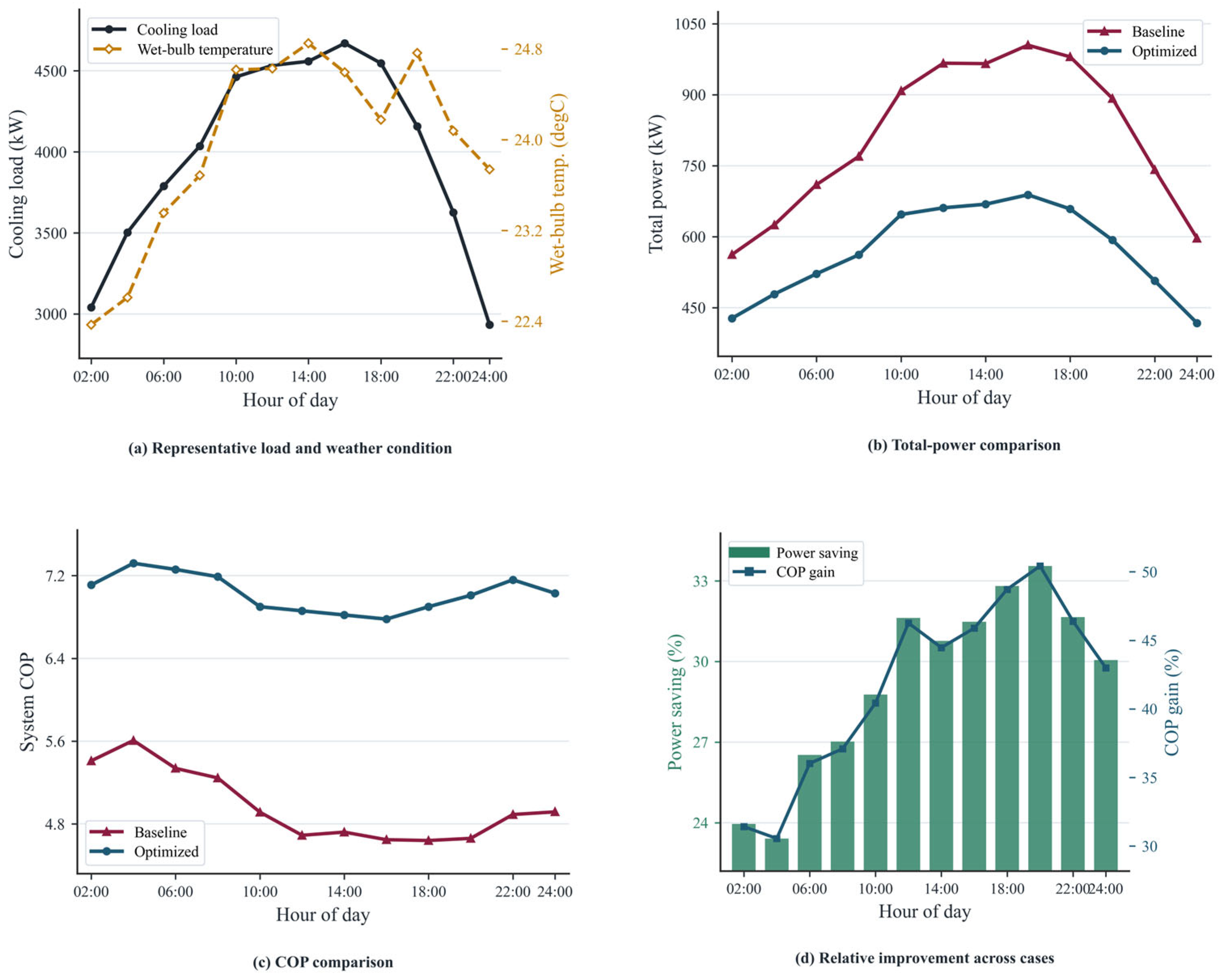
On 31 July, the cooling load varies from 2933.84 to 4669.61 kW, and the outdoor wet-bulb temperature remains the highest among the four representative days at 22.37 to 24.85 °C. Under this restrictive summer boundary, the mean total power falls from 810.17 to 569.12 kW while the mean COP rises from 4.9731 to 7.0283. Although the condenser-side burden is the most severe here, the corrected case chain still shows the largest average relative benefit in summer.

The summer trajectory is sharply shaped by condenser-side pressure. The daily load peak reaches 4669.61 kW at 16:00, while the hottest wet-bulb condition reaches 24.85 °C at 14:00. Even under this severe boundary, optimization still achieves a maximum power reduction of 33.55% at 20:00 and a maximum COP gain of 50.42% at 20:00.

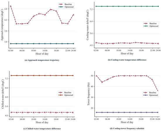
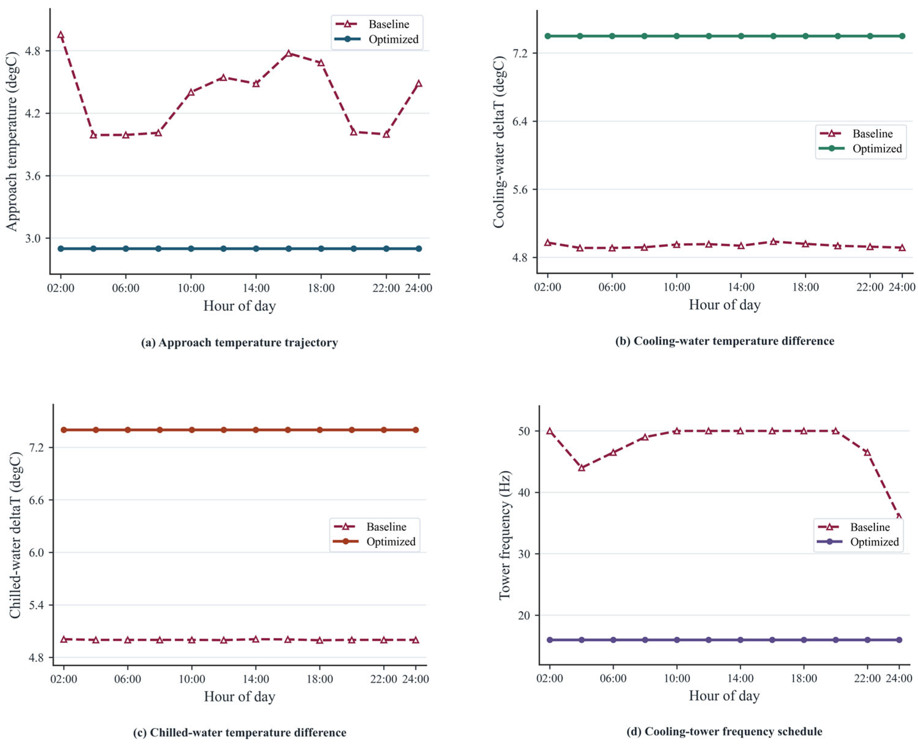
Figure 5 and Figure 6 make the summer mechanism visually explicit. By relieving condenser-side thermal stress, the coordinated strategy compresses the mean approach temperature from 4.36 to 2.90 °C and lowers tower frequency from 47.67 to 16.00 Hz. Cooling-water flow is reduced from 780.70 to 517.64 m³/h and chilled-water flow from 686.69 to 463.38 m³/h. At the component level, the mean chiller power changes by −16.20 kW, cooling-water pump power by −26.84 kW, chilled-water pump power by −22.82 kW, and cooling-tower power by −37.47 kW.

Figure 5. Hourly operating-parameter trajectories for 31 July. The summer case is the only representative day that actively compresses approach temperature to the lower bound, reflecting the strongest condenser-side pressure in the benchmark.

Figure 6. Hourly total-power and COP comparison for 31 July. Despite the harsh wet-bulb boundary, the optimized summer profile maintains the largest average relative gain across the four seasons.

Supplementary Table S3 provides the compact day summary corresponding to Figure 5 and Figure 6.

3.1.3. 15 October Representative-Day Profile

On 15 October, the cooling load varies from 2722.61 to 4461.76 kW, with an outdoor wet-bulb range of 5.37 to 10.91 °C. The baseline mean total power is 652.76 kW, and the optimized mean is 472.51 kW, while the mean COP increases from 5.8699 to 8.0450. This autumn case now sits very close to the spring pattern.

The autumn profile sits between the summer and winter extremes. The representative load crest reaches 4461.76 kW at 16:00, and the hottest wet-bulb condition reaches 10.91 °C at 16:00. A maximum power reduction of 31.75% is achieved at 20:00, whereas the weakest hour at 02:00 still yields 18.93% saving.

Figure 7 and Figure 8 show that the autumn gains emerge from synchronized multi-variable adjustment. The mean approach temperature changes only slightly from 11.43 to 11.66 °C, tower frequency falls from 31.25 to 16.00 Hz, and the cooling-water and chilled-water flow rates decline to 484.93 and 439.24 m³/h.

Figure 7. Hourly operating-parameter trajectories for 15 October. The autumn profile shows lower tower frequency and lower loop flow while the absolute cooling-water supply temperature remains close to the fitted support floor.

Figure 8. Hourly total-power and COP comparison for 15 October. Whole-system benefit remains positive across the full transition-season profile.

Supplementary Table S4 provides the compact day summary corresponding to Figure 7 and Figure 8.

3.1.4. 31 December Representative-Day Profile

On 31 December, the cooling load varies from 2566.06 to 4295.76 kW, and the outdoor wet-bulb temperature ranges from −3.71 to 1.88 °C. Under these favorable winter boundary conditions, the mean total power falls from 605.31 to 450.34 kW while the mean COP rises from 6.0503 to 8.0800. Winter, therefore, remains beneficial, but it no longer delivers the largest relative improvement because the baseline itself is already comparatively efficient.

The winter trajectory still shows consistent benefit throughout the day. The daily load peak reaches 4295.76 kW at 16:00, while the highest wet-bulb temperature reaches only 1.88 °C at 14:00. The strongest hourly power reduction reaches 29.69% at 20:00, and the maximum COP gain reaches 42.15% at 20:00.

Figure 9 and Figure 10 show that winter optimization is constrained less by condenser thermodynamics than by the support-aware cooling-water floor. The mean approach temperature shifts only from 20.98 to 21.27 °C because the optimized cooling-water supply temperature settles near 20.251 °C while wet-bulb temperatures remain close to 0 °C. Tower frequency decreases only from 18.64 to 16.00 Hz, whereas cooling-water and chilled-water flows fall from 711.64 to 464.07 m³/h and from 626.32 to 419.82 m³/h, respectively.

Figure 9. Hourly operating-parameter trajectories for 31 December, showing that the corrected winter solution settles near the fitted cooling-water support floor rather than exploiting unrealistically low condenser temperatures.

Figure 10. Hourly total-power and COP comparison for 31 December, showing positive winter gains with a smaller relative envelope than the summer case after the support-aware correction.

Supplementary Table S5 provides the compact day summary corresponding to Figure 9 and Figure 10.

Viewed together, the four representative days show a consistent but more conservative seasonal storyline. Summer now exhibits the largest average relative improvement, winter the smallest, and spring and autumn occupy an intermediate band. The common feature across spring, autumn, and winter is the convergence toward an optimized absolute cooling-water supply temperature of about 20.18–20.25 °C.

The hourly figures are embedded directly within Section 3.1.1, Section 3.1.2, Section 3.1.3 and Section 3.1.4 so that each seasonal argument can be read together with the corresponding visual evidence rather than deferred to the end of the results section.

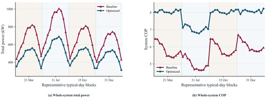
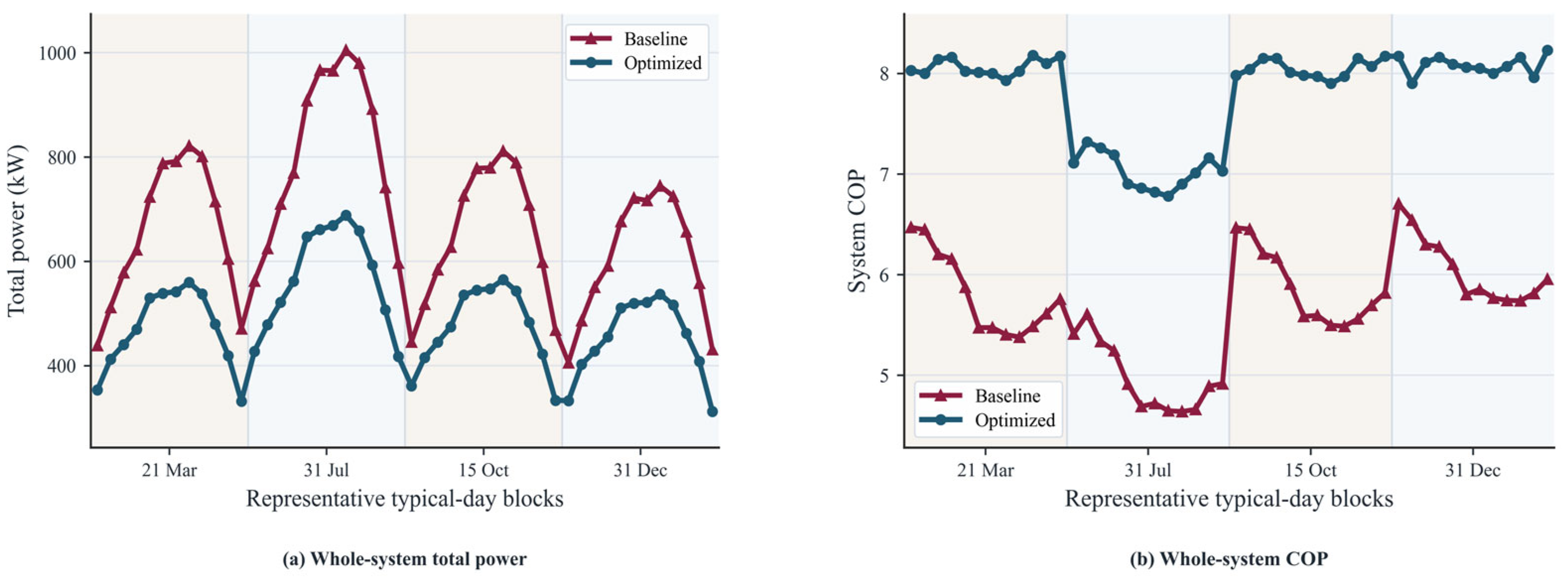
Taken together, the representative-day results can also be summarized compactly. Across the full case set, the baseline mean total power is 680.94 kW, and the optimized mean total power is 489.93 kW. The mean system COP increases from 5.6762 to 7.8042, corresponding to a mean improvement of 38.12%. Figure 11 summarizes the cross-seasonal total-power and COP comparison.

Figure 11. Cross-seasonal total-power and COP comparison across the four representative days. The optimized cases outperform the baseline in every season, with the largest average relative gain in summer and the smallest in winter after the fitted cooling-water support floor is enforced.

3.2. Peak and Off-Peak Comparison Across Seasons

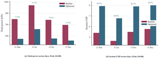
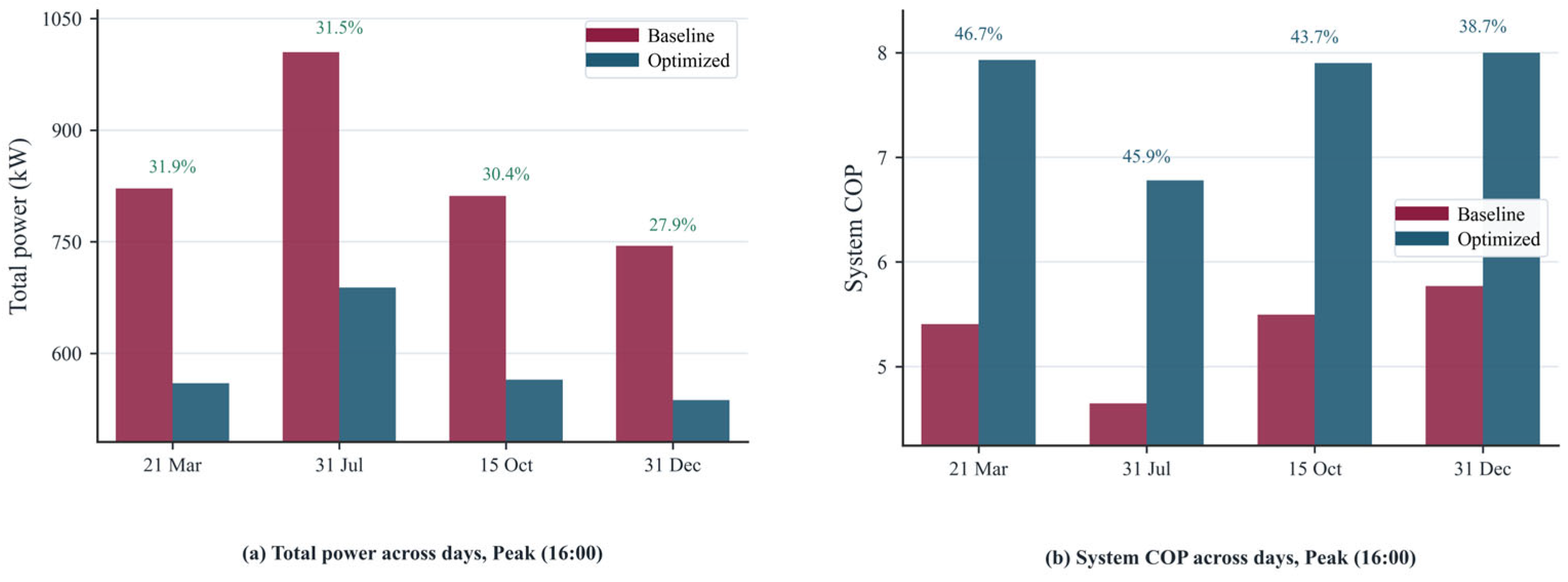
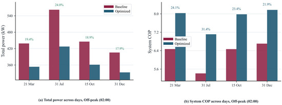
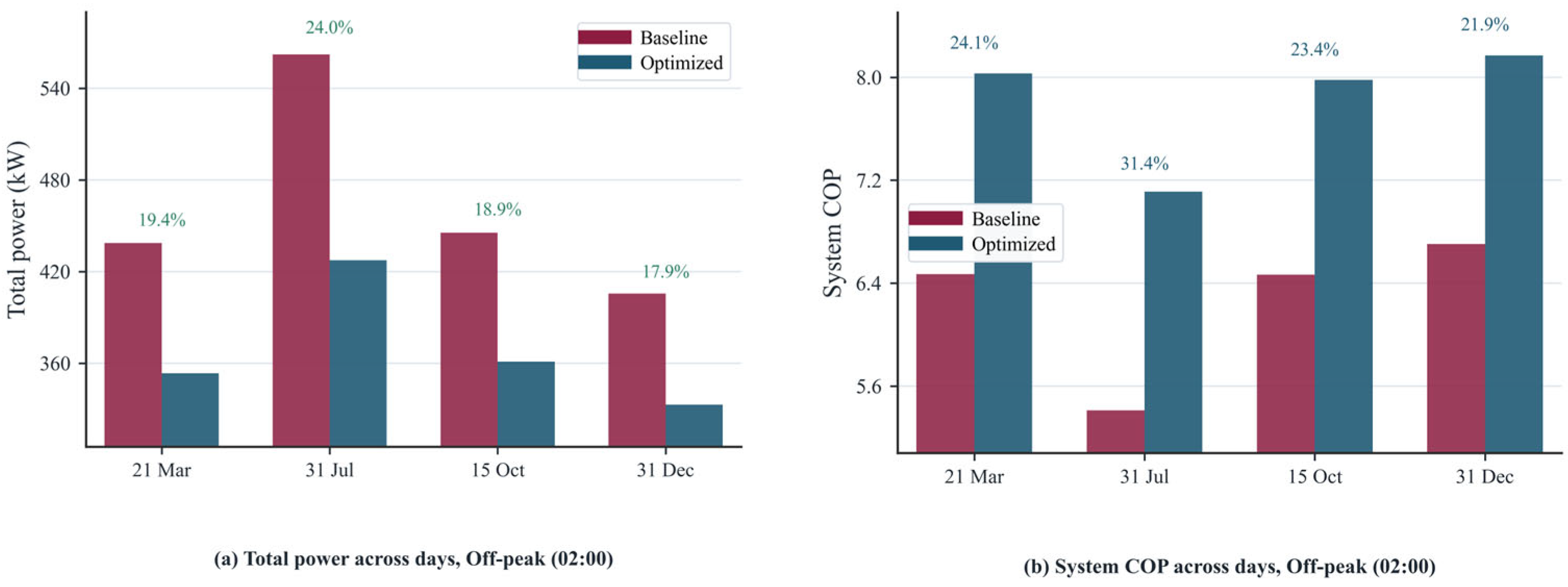
A cross-seasonal comparison at the representative 16:00 and 02:00 timestamps further clarifies the supervisory effect. Across the four 16:00 peak points, the mean power saving reaches 30.41%, and the mean COP improvement reaches 43.76%; across the four 02:00 off-peak points, the corresponding means are 20.06% and 25.21%. The strongest peak result occurs on 21 March, where power saving reaches 31.86% and COP improvement reaches 46.73%, whereas the weakest off-peak gain appears on 31 December, where power saving is 17.94%, and COP improvement is 21.86%.

These results show that optimization remains beneficial at both high and low load levels, but the ranking depends on the baseline condition rather than on a simple winter-dominant hierarchy. Peak-period gains cluster tightly across the four seasons, whereas off-peak gains narrow further because baseline power is lower and the remaining auxiliary headroom is smaller. Summer remains the most condenser-limited case, but it no longer systematically produces the weakest result after the support-aware correction.

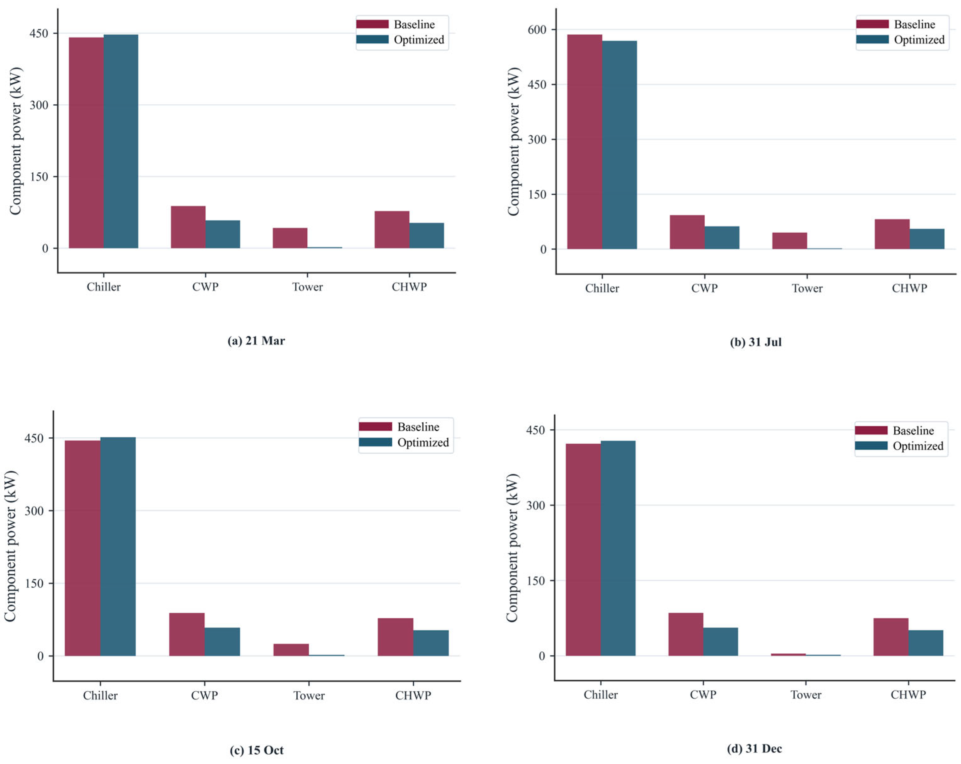
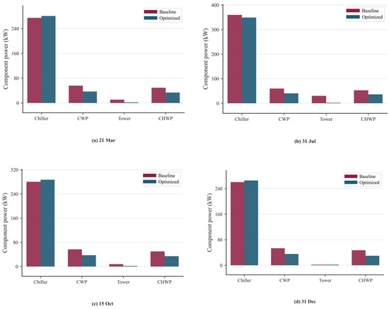
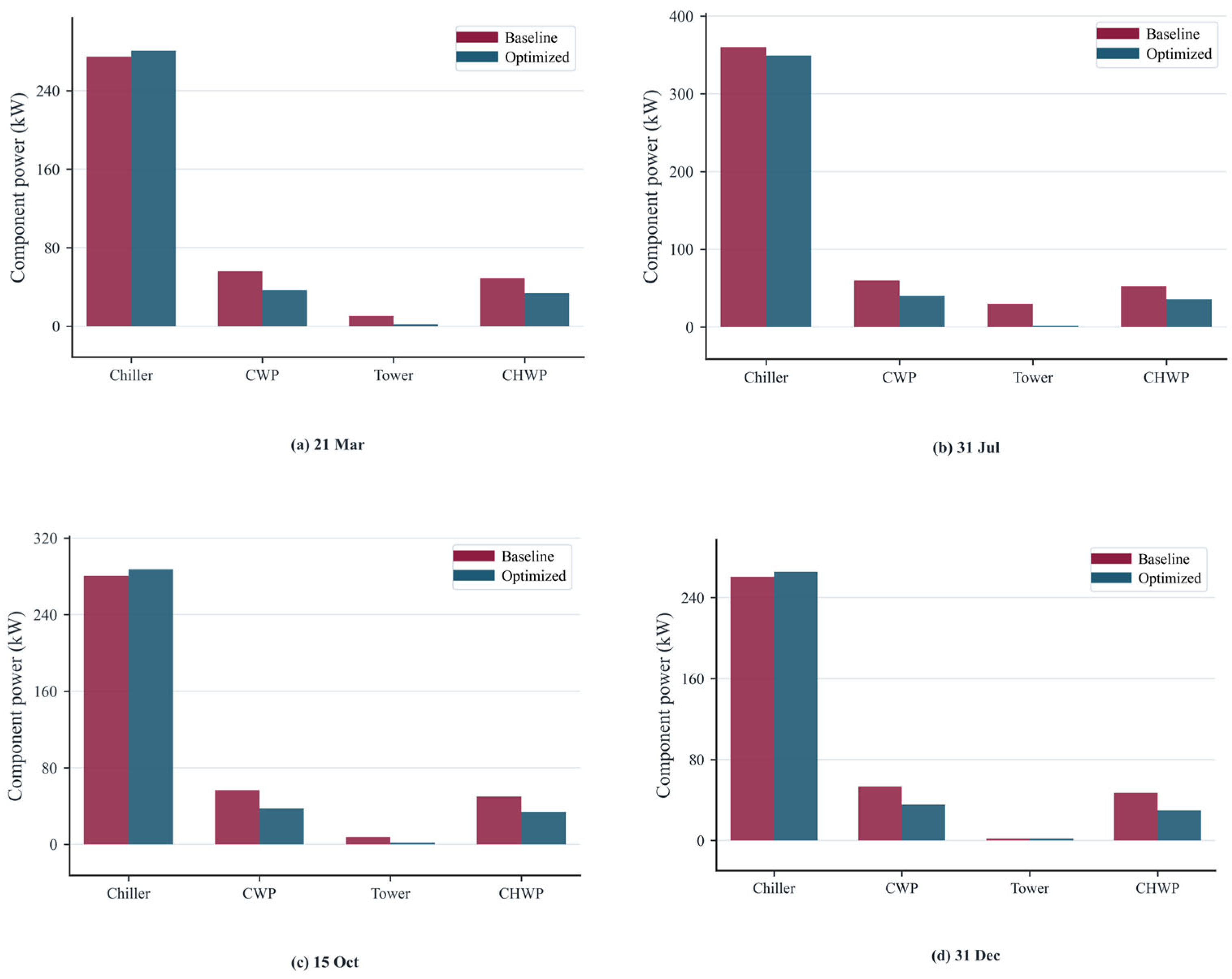
Component-level changes sharpen this corrected comparison. At the representative 16:00 peak on 31 July, cooling-tower, cooling-water pump, and chilled-water pump power decrease by −43.10, −30.57, and −26.20 kW, respectively, whereas chiller power decreases by −17.11 kW; the summer peak, therefore, remains auxiliary- and condenser-side dominated. At the strongest peak case on 21 March, the total saving is also assembled mainly by tower and pump relief (−40.22, −30.16, and −24.87 kW for tower, cooling-water pump, and chilled-water pump power), even though chiller power rises slightly by 6.16 kW. At the weakest off-peak case on 31 December, tower-side leverage is essentially exhausted (about 0.00 kW change), so the remaining gain comes primarily from pump reductions.

Supplementary Table S6 lists the detailed peak/off-peak values for the four representative days.

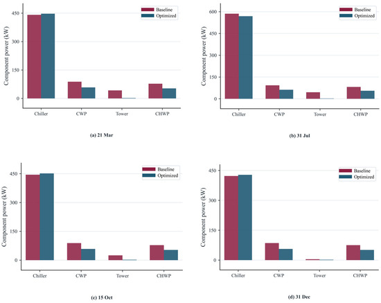
Figure 12 and Figure 13 directly support the component-level interpretation. Peak-period benefits are assembled mainly by auxiliary-side reductions rather than by uniform chiller unloading: at 21 March 16:00, tower and pump savings outweigh a slight chiller-power increase, whereas at 31 July 16:00 the condenser-side tower reduction is the single largest component. Under off-peak conditions, the weakest 31 December case occurs when the tower contribution is nearly exhausted, and the remaining benefit comes mainly from pump relief.

Figure 12. Peak-period component-power comparison across the four representative days. The largest peak savings are assembled mainly by auxiliary-side reductions, with summer dominated by condenser-side tower relief and spring delivering the strongest aggregate peak benefit after the support-aware correction.

Figure 13. Off-peak component-power comparison across the four representative days. Off-peak savings remain positive in all seasons, but winter retains the smallest residual headroom because the baseline is already efficient under favorable ambient conditions.

Figure 14 and Figure 15 translate the same comparison back to the system level. The representative peak benefits are tightly clustered, ranging from 27.87% to 31.86% in power savings, with the strongest value on 21 March. Under off-peak conditions, the gain range narrows to 17.94–23.96%, and the weakest case appears on 31 December because the favorable winter baseline leaves less room for relative improvement. Read together, these plots confirm that the supervisory strategy improves both peak and off-peak operation, but the ranking depends on the baseline condition rather than on a single fixed season label.

Figure 14. Peak-period total-power and COP comparison across the four representative days, showing positive peak-period benefits in all seasons and the strongest representative peak result on 21 March.

Figure 15. Off-peak total-power and COP comparison across the four representative days, showing positive off-peak benefits in all seasons, strongest on 31 July and weakest on 31 December.

3.3. Component Migration and Physical Interpretation

The cooling-tower power reduction should not be interpreted in isolation. On the representative summer day, tower power exhibits the largest mean percentage reduction (−95.17%), accompanied by the largest day-level chiller-power reduction (−16.20 kW), which is thermodynamically consistent with the severe condenser-side burden imposed by high wet-bulb temperature and high cooling demand. By contrast, on 31 December, the mean tower power change is only −0.69 kW and the mean chiller-power change is only −1.42 kW, while the dominant reductions occur in the cooling-water and chilled-water pumps (−25.30 and −21.08 kW). The corrected winter result is, therefore, no longer a large-chiller-saving case; it is primarily a transport-side relief case under an already favorable baseline.

This seasonal contrast makes the underlying physical point clearer. Optimization does not reduce every subsystem monotonically. Instead, it selectively redistributes thermal and hydraulic burden among chillers, pumps, and cooling towers. Under summer condenser stress, the main gain comes from aggressive auxiliary-side relief plus a moderate chiller improvement; under the milder spring, autumn, and winter cases, most of the benefit comes from reducing pump transport demand while keeping chiller power close to baseline.

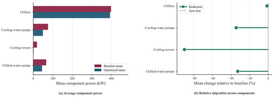
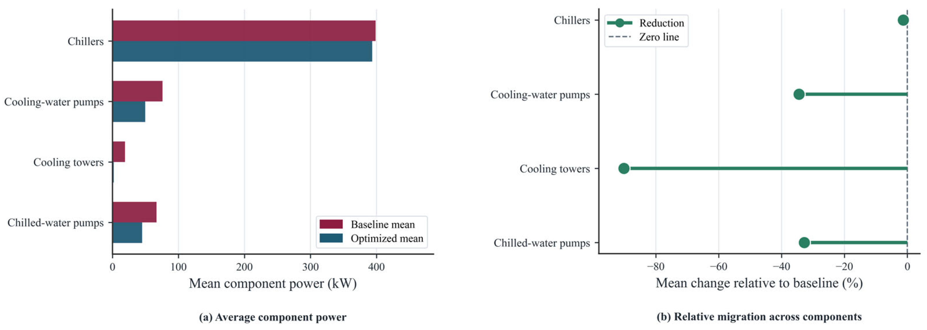
Across the full representative set, the mean chiller power falls from 398.53 to 393.38 kW, cooling-water pump power falls from 75.93 to 49.75 kW, cooling-tower power falls from 19.17 to 1.88 kW, and chilled-water pump power falls from 66.82 to 44.91 kW. Viewed together, this breakdown makes the physical interpretation more concrete: optimization is not uniformly suppressing every device. It is selectively reallocating effort among compressors, pumps, and towers to reach a lower whole-system power point under the same load-weather condition.

This interpretation is also why cooling-tower savings are discussed only through a system-total perspective. A very large reduction in tower or pump power is meaningful only if the accompanying chiller response does not erase the gain. The component table and figure are, therefore, intended as a diagnostic layer: they reveal where the modeled savings originate, whether one auxiliary-device reduction is being offset elsewhere, and why the final assessment of performance must still rest on total power and COP. The corresponding component-level averages are summarized in Table 3, and the aggregate migration pattern is visualized in Figure 16.

Table 3. Component-level average power migration between baseline and optimized cases.

Component	Baseline Mean (kW)	Optimized Mean (kW)	Mean Change (kW)	Mean Change (%)	Cases with Lower Optimized Power
Chillers	398.53	393.38	−5.15	−1.29	26/48
Cooling-water pumps	75.93	49.75	−26.18	−34.48	48/48
Cooling towers	19.17	1.88	−17.28	−90.17	43/48
Chilled-water pumps	66.82	44.91	−21.90	−32.78	48/48

Figure 16. Component-level power migration under optimized controls, illustrating that the final saving is assembled mainly through pump and cooling-tower relief, with chiller-power changes remaining secondary and season dependent.

3.4. Surrogate Model Accuracy and Uncertainty

Table 4 reports the MAPE, RMSE, and R2 for every fitted component model. The chiller-power surrogates remain within 1.7875–2.2030% MAPE, while the pump power models remain within 0.0982–0.1112% MAPE, indicating that the main power-consumption channels are captured with stable accuracy. Across the full model set, the numerically highest MAPE appears in the CT-3 fan-power fit at 16.3082%, yet this auxiliary power channel still retains a relatively small RMSE of 0.686667 kW and an R2 of 0.986955. By contrast, the most decision-relevant uncertainty lies in the cooling-tower heat-rejection models because they enter the heat-balance check directly; after replacing the old three-parameter formula with a second-order interaction surrogate, their MAPE is reduced to 0.4926–0.5378%, and R2 rises to 0.995206–0.998866. Because the cooling-tower heat-rejection model directly affects the feasibility screen, the optimization results should still be interpreted as simulation evidence with model-form uncertainty rather than as experimentally validated dispatch commands.

Table 4. (a). Fitted surrogate model descriptors, training basis, and sample counts used in the uncertainty discussion. (b). Fitted surrogate model accuracy metrics used in the uncertainty discussion.

(a)
Model	Inputs	Fitting Method	Samples
Chilled-water pump 1 power	Chilled-water flow1	Quadratic polynomial	8760
Chilled-water pump 2 power	Chilled-water flow2	Quadratic polynomial	8760
Chilled-water pump 3 power	Chilled-water flow3	Quadratic polynomial	8030
Chiller 1 power	Qe1, Cooling-water supply temperature, Chilled-water supply temperature	8-parameter nonlinear fit	43,796
Chiller 2 power	Qe2, Cooling-water supply temperature, Chilled-water supply temperature	8-parameter nonlinear fit	43,796
Chiller 3 power	Qe3, Cooling-water supply temperature, Chilled-water supply temperature	8-parameter nonlinear fit	39,785
Cooling pump 1 power	Cooling-water flow1	Quadratic polynomial	8760
Cooling pump 2 power	Cooling-water flow2	Quadratic polynomial	8760
Cooling pump 3 power	Cooling-water flow3	Quadratic polynomial	8030
Cooling tower 1 heat rejection	Cooling-water flow1, Cooling-tower frequency1, Cooling-water supply temperature, Outdoor wet-bulb temperature	Second-order interaction polynomial	8760
Cooling tower 1 fan power	Cooling-tower frequency1	Fourth-order polynomial	8760
Cooling tower 2 heat rejection	Cooling-water flow2, Cooling-tower frequency2, Cooling-water supply temperature, Outdoor wet-bulb temperature	Second-order interaction polynomial	8760
Cooling tower 2 fan power	Cooling-tower frequency2	Fourth-order polynomial	8760
Cooling tower 3 heat rejection	Cooling-water flow3, Cooling-tower frequency3, Cooling-water supply temperature, Outdoor wet-bulb temperature	Second-order interaction polynomial	8030
Cooling tower 3 fan power	Cooling-tower frequency3	Fourth-order polynomial	8030
(b)
Model	MAPE (%)	RMSE	R2
Chilled-water pump 1 power	0.1094	0.029296	0.999856
Chilled-water pump 2 power	0.1094	0.029293	0.999856
Chilled-water pump 3 power	0.1112	0.028765	0.999962
Chiller 1 power	2.2030	4.904666	0.962220
Chiller 2 power	2.2030	4.904666	0.962220
Chiller 3 power	1.7875	4.278413	0.973363
Cooling pump 1 power	0.0982	0.029661	0.999885
Cooling pump 2 power	0.0982	0.029658	0.999886
Cooling pump 3 power	0.0993	0.029005	0.999970
Cooling tower 1 heat rejection	0.5121	11.932910	0.995206
Cooling tower 1 fan power	1.3110	0.099172	0.999725
Cooling tower 2 heat rejection	0.4926	10.662587	0.996172
Cooling tower 2 fan power	1.3110	0.099172	0.999725
Cooling tower 3 heat rejection	0.5378	10.399467	0.998866
Cooling tower 3 fan power	16.3082	0.686667	0.986955

The remaining cooling-tower heat-rejection-model error is also physically understandable. Heat rejection depends on coupled variation in water flow, fan frequency, cooling-water return temperature, and outdoor wet-bulb temperature, so it is the most interaction-sensitive part of the surrogate stack. Even after the model-form upgrade, the corresponding RMSE still spans 10.399467 to 11.932910 kW, which means that this surrogate remains the principal constraint-side uncertainty whenever the optimized cases approach pump upper limits or tight heat-balance margins. By comparison, the tower fan models span 1.3110–16.3082% MAPE, and the elevated CT-3 fan percentage error is better understood as a low-load auxiliary-fit issue than as the dominant source of system-level energy uncertainty.

For this reason, uncertainty is not reduced here to a single headline accuracy number. The fit table also reports the sample count, fitting method, input columns, and input range so that the reader can distinguish a seemingly large percentage error on a low-power auxiliary channel from a decision-relevant constraint-side error in heat rejection. This distinction matters directly for interpretation: the largest percentage deviation and the most consequential uncertainty for optimization decisions are not necessarily the same thing, and the discussion, therefore, treats them separately instead of collapsing them into one scalar claim.

3.5. jDE Versus Grid Search and Constraint Diagnostics

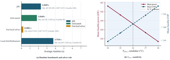
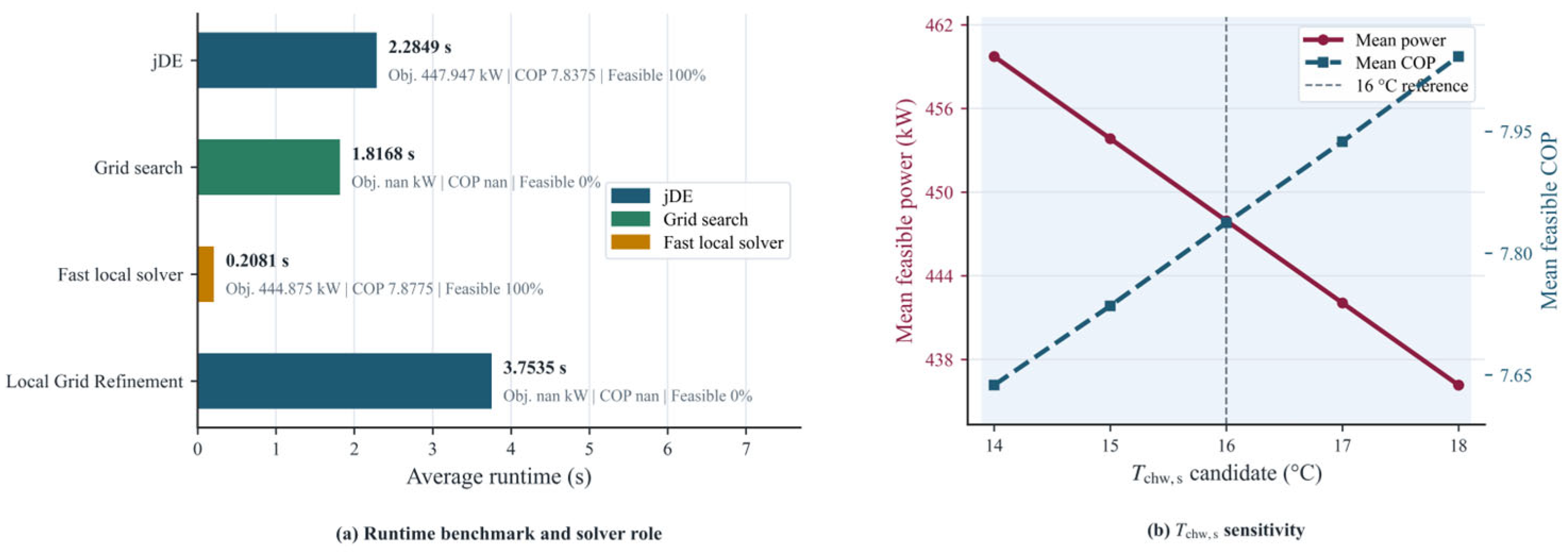
The runtime comparison is used here to separate solver roles rather than to declare a universal winner. On the representative benchmark, jDE requires about 2.2849 s on average and returns feasible solutions in 100.00% of cases. The fast local solver is much faster at 0.2081 s and is also feasible in 100.00% of cases, with a slightly lower mean objective (444.875 kW versus 447.947 kW for jDE). However, its behavior remains initialization-dependent and is, therefore, treated as an acceleration-oriented reference rather than as a general replacement for global search. By contrast, the current coarse grid search and deterministic local lattice return 0.00% feasible cases. In this corrected manuscript, they are retained only as transparency checks on discretization and neighborhood design, not as competing optimizers. The corresponding runtime, objective, and feasibility statistics are summarized in Table 5.

Table 5. (a). Runtime, objective, and COP summary for the exported optimization algorithms. (b). Feasible rate, search scope, and role definition for the exported optimization algorithms.

(a)
Algorithm	Runtime (s)	Mean Objective (kW)	Mean COP
jDE	2.2849	447.947	7.8375
Grid search	1.8168	NA	NA
Deterministic local lattice	3.7535	NA	NA
Fast local solver	0.2081	444.875	7.8775
(b)
Algorithm	Feasible Rate (%)	Search Scope	Role in Study
jDE	100.00	Global stochastic	Primary optimizer
Grid search	0.00	Coarse lattice	Deterministic cross-check
Deterministic local lattice	0.00	jDE-centered local lattice	Neighborhood cross-check
Fast local solver	100.00	Fast local multi-start	Acceleration-oriented reference

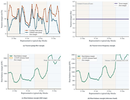
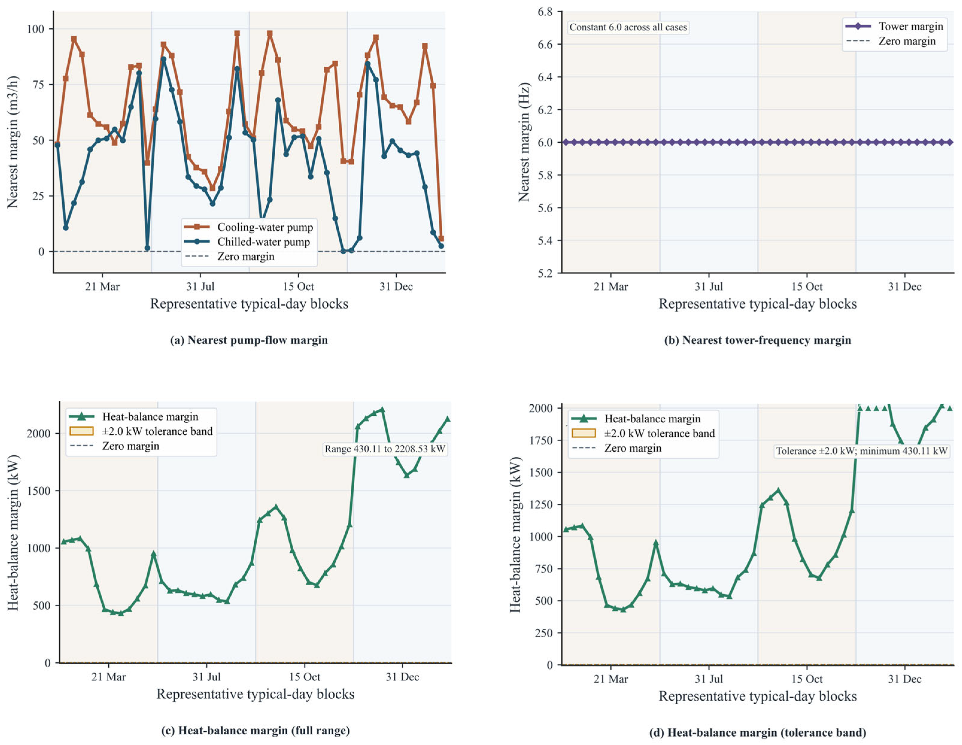
In Table 5, NA denotes not applicable because no feasible solution was obtained for the corresponding algorithm. The constraint analysis further shows that all 48 cases in the four-season representative batch remain within the configured operational envelope. The minimum upper-margin values are 5.7292 m3/h for cooling-water pumps and 0.1361 m3/h for chilled-water pumps, while the minimum cooling-tower frequency upper margin is 34.0 Hz and the lower margin remains a constant 6.0 Hz across all 48 cases. The heat-balance margin spans 430.1102 to 2208.5285 kW. Figure 17 visualizes the pump-flow margins, the tower-frequency headroom, and the heat-balance residual on both the full scale and within the configured ±2.0 kW tolerance band. Because any case violating these checks would be discarded before reporting, the positive headroom confirms that the corrected savings are not obtained by underserving the cooling load or stepping outside the configured operating envelope. Read together, these complementary views support the feasibility of the representative-case set, although broader annual validation and field-deployment evidence remain outside the present scope.

Figure 17. Constraint margin diagnostics under the configured operational limits. The corrected representative batch preserves positive pump and tower headroom, as well as positive heat-balance margins across all 48 cases.

The solver benchmark should, therefore, be read as a role differentiation rather than as an absolute league table. The fast local solver is attractive when a good initialization is already available, but local methods can still miss lower-power regions in a broader nonconvex supervisory problem. jDE remains the primary optimizer because it preserves global search behavior without manual lattice redesign. The infeasible grid-based checks are still useful diagnostically: they show how quickly feasibility can collapse when discretization or neighborhood design is misaligned with the true coupled feasible region.

3.6. Sensitivity, Actuator Variation, and Comparison with Related Studies

A chilled-water supply temperature sensitivity analysis over 14–18 °C is included to reassess the conventional 16 °C initial setting across the supported interval. The retrained chiller dataset contains approximately one year of hourly samples at each nominal setpoint: 8759 cases at 14 °C, 8759 at 15 °C, 8760 at 16 °C, 8759 at 17 °C, and 8759 at 18 °C. The fitted chilled-water supply support, therefore, spans approximately 14.0–18.0 °C. Each of the five candidate setpoints remains feasible in all four evaluated sensitivity cases. Over this range, the mean feasible power decreases from 459.735 kW at 14 °C to 436.160 kW at 18 °C, while the mean feasible COP rises from 7.6375 to 8.0425. Table 6 summarizes the fitted-range coverage labels and the mean feasible performance across the five candidate setpoints.

Table 6. (a). Chilled-water supply temperature sensitivity summary with fitted-range coverage labels. Part 1 of 2. (b). Chilled-water supply temperature sensitivity summary with fitted-range coverage labels. Part 2 of 2.

(a)
Tchw,s Candidate (°C)	In Fitted Range	Mean Power (kW)	Mean COP	Feasible Cases	Result Available	Evidence Level	Constraint Status
14	Yes	459.735	7.6375	4/4	Yes	Within fitted range	satisfied
15	Yes	453.843	7.7350	4/4	Yes	Within fitted range	satisfied
16	Yes	447.947	7.8375	4/4	Yes	Within fitted range	satisfied
17	Yes	442.055	7.9375	4/4	Yes	Within fitted range	satisfied
18	Yes	436.160	8.0425	4/4	Yes	Within fitted range	satisfied
(b)
Tchw,s Candidate (°C)				Manuscript Use
14				Quantitative
15				Quantitative
16				Quantitative
17				Quantitative
18				Quantitative

This analysis also clarifies where the quantitative evidence begins and ends. Because the chiller models were retrained with additional 14/15/17/18 °C hourly data, the full 14–18 °C interval can be discussed as an in-support quantitative sweep for the chiller-sensitive portion of the optimization. At the same time, the pump and tower models were not retrained on a separate 14–18 °C dataset, so the sensitivity results are better understood as a controlled supervisory comparison within the present surrogate stack rather than as standalone operating guidance. Figure 18 summarizes the runtime benchmark and chilled-water-supply-temperature sensitivity results.

Figure 18. Runtime comparison and chilled-water-supply-temperature sensitivity within the fitted support range. The sensitivity panel uses only the retrained 14–18 °C chiller domain and shows monotonically lower mean power at higher chilled-water supply temperatures within the evaluated cases.

Adjacent-period control-movement statistics provide a first indication of whether the pointwise optimum is dynamically reasonable. Across the full representative sequence, the maximum step changes are 9.6 °C for the approach temperature, 0.0 °C for the cooling-water temperature difference, 0.6 °C for the chilled-water temperature difference, and 0.0 Hz for the cooling-tower frequency. The large 9.6 °C excursion is driven mainly by transitions between seasonal representative days rather than by within-day oscillation; within a single day, the maximum approach step is 3.0 °C. The remaining channels are essentially flat because the corrected optimum repeatedly selects the same cooling-water and tower settings. Because those two channels collapse into degenerate zero-variation traces in the corrected batch, their diagnostics are summarized directly in the text rather than retained as a separate low-information figure. Read in this way, the revised results no longer support the earlier appearance of strong within-day overcontrolling; most of the visible excursion comes from concatenating different seasonal representative days. This substantially mitigates actuator-wear concerns for the representative scenarios, although explicit rate penalties, hysteresis rules, or smoothing constraints would still be advisable before any practical online deployment.

Accordingly, energy savings alone are not sufficient to establish implementability. The revised trajectories are markedly smoother within each representative day than the earlier draft suggested, which weakens the concern that pumps, fans, or valves would be driven by large, repeated oscillations. Even so, a pointwise steady-state optimum may still require temporal regularization before it can be translated into a continuous supervisory control policy with acceptable actuator behavior.

The mean COP improvement of 38.12% and mean power reduction of 27.34% reflect control-only optimization gains under a simulated baseline; no hardware retrofit is introduced in this study. The relatively large COP uplift is, therefore, baseline-sensitive rather than hardware-driven: in the reproduced baseline, fixed supervisory settings around the original 16 °C chilled-water supply logic and conservative condenser-side operation suppress efficiency in part of the benchmark, whereas the optimizer recovers part of that headroom by coordinating chillers, pumps, and towers within the fitted support. Placed against the cited literature, these values remain substantial but no longer implausibly extreme. Fan et al. [21] reported around 14.3% maximum energy saving for MPC-based optimization of a chiller plant with a water-side economizer, whereas Wang et al. [20] reported about 37% energy saving for a DRL-based broader building-HVAC benchmark. The present mean power reduction, therefore, sits above the closer single-plant supervisory benchmark and below the broader DRL benchmark. This position is consistent with a simulation-only plant-level study that coordinates multiple coupled subsystems under one fixed topology, and it should not be read as a universal field expectation for already well-tuned plants.

Table 7 compares the present study with representative optimization studies that are already cited in the manuscript. The comparison is used to distinguish the differences in plant scope, control leverage, objective definition, and validation basis when interpreting the reported energy-saving levels. In particular, several reference studies optimize a narrower subset of plant decisions, whereas the present benchmark coordinates chiller, pump, and tower actions together; this helps explain why the reported saving can exceed some narrower supervisory studies without implying direct superiority across heterogeneous setups.

Table 7. (a). Representative optimization studies, benchmark scope, and reported energy-performance gain. (b). Validation basis and positioning notes for the representative studies cited in the manuscript.

(a)
Study	Benchmark Scope	Reported Saving/Gain
Trautman et al. [9] (as cited in the Introduction)	Whole chilled-water system; MPC-style supervisory coordination	Approximately 10% energy saving
Wijaya et al. [7] (as cited in the Introduction)	Variable-frequency chilled-water-pump optimization	Approximately 12% energy saving
Deepika and Dhanya [24] (as cited in the Introduction)	Cloud-data center multi-objective predictive optimization	About 10% energy consumption reduction
Fan et al. [21] (Section 3.6 benchmark sentence)	MPC-based optimization of a chiller plant with a water-side economizer	Around 14.3% maximum energy saving
Wang et al. [20] (Section 3.6 benchmark sentence)	DRL-based benchmark for a broader building-HVAC supervisory problem	About 37% energy saving
Present study	Nanjing TRNSYS three-chiller water-side plant with jDE plus deterministic benchmark	Mean total-power saving 27.34%; mean COP improvement 38.12%
(b)
Study	Validation Basis	Key Note
Trautman et al. [9] (as cited in the Introduction)	Literature benchmark cited in the retained review chain	Whole-system reference, but the present manuscript reports constraint, runtime, and provenance evidence more explicitly.
Wijaya et al. [7] (as cited in the Introduction)	Component-focused optimization literature	Useful transport-side benchmark, but narrower than the present whole-plant scope.
Deepika and Dhanya [24] (as cited in the Introduction)	Predictive optimization benchmark with a different objective set	Relevant for objective design, but not directly comparable to the present single-objective plant benchmark.
Fan et al. [21] (Section 3.6 benchmark sentence)	Representative supervisory control benchmark used for discussion	A closer supervisory benchmark than broader building-HVAC control studies.
Wang et al. [20] (Section 3.6 benchmark sentence)	Broader HVAC-control literature rather than the same plant topology	Used only to position result magnitude while keeping topology and validation differences explicit.
Present study	48 reproduced simulation/optimization cases across four representative seasonal days	Control-only optimization with explicit fit metrics, source audit, constraint margins, sensitivity analysis, and control-movement discussion; no field validation claimed.

Supplementary Tables S7 and S8 provide additional detail for this comparison. Supplementary Table S7 extends the literature comparison, whereas Supplementary Table S8 summarizes the relationship among baseline simulation outputs, optimized reruns, model-training support, and configured constraints.

Taken together, the results define not only the magnitude of the simulation-based saving but also its support range, computational cost, constraint headroom, and control-smoothness implications.

4. Conclusions

This study developed a simulation-based plant-level optimization framework for a Nanjing data center chilled-water plant by combining TRNSYS operating scenarios, fitted surrogate component models, and a jDE search. Across 48 representative operating cases selected from four seasonal days, the corrected optimized operation reduces total power by 17.24–33.55%, relative to matched baseline values, with a mean saving of 27.34%, and increases system COP by 20.78–50.42%, with a mean improvement of 38.12%.

The central conclusion is that the reported benefit is genuinely system level. This saving is primarily achieved through the coordinated selective redistribution of compressor and auxiliary loads rather than through uniform reductions in every component. All reported gains are obtained while the representative cases remain inside the configured cooling-duty and heat-balance feasibility checks. After enforcing the fitted cooling-water support floor, the day-level relative gain is largest in summer and smallest in winter, while representative peak and off-peak rankings vary with the baseline condition; a blanket winter-best claim is, therefore, no longer supported.

This study also shows the methodological value of keeping the plant structure explicit during optimization. Because the objective is decomposed into component surrogates and then checked against configuration-level bounds, the analysis can explain not only how much power is saved, but also where the savings are created and under what conditions they remain feasible. From the solver perspective, jDE remains the primary global optimizer for the present continuous constrained problem, the fast local solver serves as an acceleration reference, and the infeasible grid-based checks function only as diagnostic benchmarks.

Model-fit statistics, runtime comparisons, chilled-water supply temperature sensitivity, and constraint margin diagnostics further define the evidential scope of the method. All 48 cases in the representative seasonal batch satisfy the configured constraint checks, with pump and fan headroom preserved, heat-balance margins remaining positive, and optimized cooling-water supply temperatures staying within 20.05–27.75 °C above the fitted floor of 19.9274 °C. These checks mean that the reported savings are not obtained by underserving the reproduced IT-side cooling load. Meanwhile, the retrained chiller models place the full 14–18 °C sensitivity sweep inside the fitted chilled-water supply domain.

These conclusions should, therefore, be read as simulation-based evidence for supervisory optimization potential rather than as measured field performance. Future work should extend validation with measured operating data and hardware-in-the-loop or physical test-platform experiments under sensor noise and actuator inertia, broaden training support beyond the current fitted chilled-water supply range, and introduce temporal smoothing or multi-objective formulations so that energy savings, control smoothness, and equipment actuation limits can be addressed within the same supervisory framework.

References

- Masanet, E.; Shehabi, A.; Lei, N.; Smith, S.; Koomey, J. Recalibrating Global Data Center Energy-Use Estimates. Science 2020, 367, 984–986. [Google Scholar] [CrossRef] [Scilit]
- Zhang, Q.; Meng, Z.; Hong, X.; Zhan, Y.; Liu, J.; Dong, J.; Bai, T.; Niu, J.; Deen, M.J. A Survey on Data Center Cooling Systems: Technology, Power Consumption Modeling and Control Strategy Optimization. J. Syst. Archit. 2021, 119, 102253. [Google Scholar] [CrossRef] [Scilit]
- Li, J.; Li, Z. Model-Based Optimization of Free Cooling Switchover Temperature and Cooling Tower Approach Temperature for Data Center Cooling System with Water-Side Economizer. Energy Build. 2020, 227, 110407. [Google Scholar] [CrossRef] [Scilit]
- Zhou, C.; Gao, D.; Rivalin, L.; Grier, A.; Ramirez, G.A.; Fabian, J. Simulator-Based Reinforcement Learning for Data Center Cooling Optimization. Engineering at Meta. 10 September 2024. Available online: https://engineering.fb.com/2024/09/10/data-center-engineering/simulator-based-reinforcement-learning-for-data-center-cooling-optimization/ (accessed on 22 March 2026).
- Lazic, N.; Lu, T.; Boutilier, C.; Ryu, M.K.; Wong, E.J.; Roy, B.; Imwalle, G. Data Center Cooling Using Model-Predictive Control. In Proceedings of the Thirty-Second Conference on Neural Information Processing Systems (NeurIPS 2018), Montreal, QC, Canada, 3–8 December 2018; pp. 3818–3827. [Google Scholar]
- Fang, Q.; Wang, J.; Zhu, H.; Gong, Q. Using Model Predictive Control in Data Centers for Dynamic Server Provisioning. IFAC Proc. Vol. 2014, 47, 9635–9642. [Google Scholar] [CrossRef] [Scilit]
- Kelvin Wijaya, T.; Sholahudin; Idrus Alhamid, M.; Saito, K.; Nasruddin, N. Dynamic Optimization of Chilled Water Pump Operation to Reduce HVAC Energy Consumption. Therm. Sci. Eng. Prog. 2022, 36, 101512. [Google Scholar] [CrossRef] [Scilit]
- Chang, Q.; Huang, Y.; Liu, K.; Xu, X.; Zhao, Y.; Pan, S. Optimization Control Strategies and Evaluation Metrics of Cooling Systems in Data Centers: A Review. Sustainability 2024, 16, 7222. [Google Scholar] [CrossRef] [Scilit]
- Trautman, N.; Razban, A.; Chen, J. Overall Chilled Water System Energy Consumption Modeling and Optimization. Appl. Energy 2021, 299, 117166. [Google Scholar] [CrossRef] [Scilit]
- Zhan, X.; Zhu, X.; Cheng, P.; Hu, X.; He, Z.; Geng, H.; Leng, J.; Zheng, H.; Liu, C.; Hong, T.; et al. Data Center Cooling System Optimization Using Offline Reinforcement Learning. In Proceedings of the Thirteenth International Conference on Learning Representations (ICLR 2025), Singapore, 24–28 April 2025; Available online: https://arxiv.org/abs/2501.15085 (accessed on 22 March 2026).
- Mughees, N.; Jaffery, M.H.; Mughees, A.; Ansari, E.A.; Mughees, A. Reinforcement Learning-Based Composite Differential Evolution for Integrated Demand Response Scheme in Industrial Microgrids. Appl. Energy 2023, 342, 121150. [Google Scholar] [CrossRef] [Scilit]
- Lin, J.; Lin, W.; Lin, W.; Liu, T.; Wang, J.; Jiang, H. Multi-Objective Cooling Control Optimization for Air-Liquid Cooled Data Centers Using TCN-BiGRU-Attention-Based Thermal Prediction Models. Build. Simul. 2024, 17, 2145–2161. [Google Scholar] [CrossRef] [Scilit]
- Peng, L.; Yuan, Z.; Dai, G.; Wang, M.; Tang, Z. Reinforcement Learning-Based Hybrid Differential Evolution for Global Optimization of Interplanetary Trajectory Design. Swarm Evol. Comput. 2023, 81, 101351. [Google Scholar] [CrossRef] [Scilit]
- Chen, Z.; Chen, Y.; Yang, C. Impacts of Large Chilled Water Temperature Difference on Thermal Comfort, Equipment Sizes, and Energy Saving Potential. J. Build. Eng. 2022, 49, 104069. [Google Scholar] [CrossRef] [Scilit]
- Wei, X.; Xu, G.; Kusiak, A. Modeling and Optimization of a Chiller Plant. Energy 2014, 73, 898–907. [Google Scholar] [CrossRef] [Scilit]
- Lin, J.; Lin, W.; Lin, W.; Wang, J.; Jiang, H. Thermal Prediction for Air-Cooled Data Center Using Data Driven-Based Model. Appl. Therm. Eng. 2022, 217, 119207. [Google Scholar] [CrossRef] [Scilit]
- Ogura, M.; Wan, J.; Kasahara, S. Model Predictive Control for Energy-Efficient Operations of Data Centers with Cold Aisle Containments. IFAC-PapersOnLine 2018, 51, 209–214. [Google Scholar] [CrossRef] [Scilit]
- Liao, J.; Xie, X.; Nemer, H.; Claridge, D.E.; Culp, C.H. A Simplified Methodology to Optimize the Cooling Tower Approach Temperature Control Schedule in a Cooling System. Energy Convers. Manag. 2019, 199, 111950. [Google Scholar] [CrossRef] [Scilit]
- Martinez-Garcia, F.; Badawy, G.; Kheradmandi, M.; Down, D.G. Adaptive Predictive Control of a Data Center Cooling Unit. Control Eng. Pract. 2021, 107, 104674. [Google Scholar] [CrossRef] [Scilit]
- Wang, H.; Chen, X.; Vital, N.; Duffy, E.; Razi, A. Energy Optimization for HVAC Systems in Multi-VAV Open Offices: A Deep Reinforcement Learning Approach. Appl. Energy 2024, 356, 122354. [Google Scholar] [CrossRef] [Scilit]
- Fan, C.; Zhou, X. Model-Based Predictive Control Optimization of Chiller Plants with Water-Side Economizer System. Energy Build. 2023, 278, 112633. [Google Scholar] [CrossRef] [Scilit]
- Chaerun Nisa, E.; Kuan, Y.-D. Comparative Assessment to Predict and Forecast Water-Cooled Chiller Power Consumption Using Machine Learning and Deep Learning Algorithms. Sustainability 2021, 13, 744. [Google Scholar] [CrossRef] [Scilit]
- Chen, X.; Tu, R.; Yang, X. Parameter Prediction Optimization of Data Center’s Heat Dissipation System Using Machine Learning Algorithms. Appl. Therm. Eng. 2023, 232, 121047. [Google Scholar] [CrossRef] [Scilit]
- Deepika, T.; Dhanya, N.M. Multi-Objective Prediction-Based Optimization of Power Consumption for Cloud Data Centers. Arab. J. Sci. Eng. 2023, 48, 1173–1191. [Google Scholar] [CrossRef] [Scilit]
- Zhao, J.; Chen, Z.; Li, H.; Liu, D. A Model Predictive Control for a Multi-Chiller System in Data Center Considering Whole System Energy Conservation. Energy Build. 2024, 324, 114919. [Google Scholar] [CrossRef] [Scilit]
- Yang, Y.; Bjørnskov, J.; Jradi, M. Optimizing HVAC Systems with Model Predictive Control: Integrating Ontology-Based Semantic Models for Energy Efficiency and Comfort. Front. Energy Res. 2025, 13, 1542107. [Google Scholar] [CrossRef] [Scilit]
- Hou, J.; Li, X.; Wan, H.; Sun, Q.; Dong, K.; Huang, G. Real-Time Optimal Control of HVAC Systems: Model Accuracy and Optimization Reward. J. Build. Eng. 2022, 50, 104159. [Google Scholar] [CrossRef] [Scilit]
- Liang, X.; Liu, Y.; Chen, S.; Li, X.; Jin, X.; Du, Z. Physics-Informed Neural Network for Chiller Plant Optimal Control with Structure-Type and Trend-Type Prior Knowledge. Appl. Energy 2025, 390, 125857. [Google Scholar] [CrossRef] [Scilit]
- Yang, S.; Yu, J.; Gao, Z.; Zhao, A. Energy-Saving Optimization of Air-Conditioning Water System Based on Data-Driven and Improved Parallel Artificial Immune System Algorithm. Energy Convers. Manag. 2023, 283, 116902. [Google Scholar] [CrossRef] [Scilit]
- Wang, L.; Lee, E.W.M.; Yuen, R.K.K.; Feng, W. Cooling Load Forecasting-Based Predictive Optimisation for Chiller Plants. Energy Build. 2019, 198, 261–274. [Google Scholar] [CrossRef] [Scilit]
- Jain, V.; Alleyne, A.G. Model-Based Optimization of Vapor Compression Refrigeration Cycle. Energy 2013, 58, 95–104. [Google Scholar] [CrossRef] [Scilit]
- Zhao, Y.; Xia, L.; Ma, Y.; Yu, J.; Zhang, M. Integrative Thermodynamic Optimization of a Vapor Compression Refrigeration System Based on Dynamic System Responses. Appl. Therm. Eng. 2018, 133, 496–505. [Google Scholar] [CrossRef] [Scilit]
- Ding, T.; Deng, K.; Yao, Y.; Li, C.; Gao, R. Proper Orthogonal Decomposition for Reduced Order Dynamic Modeling of Vapor Compression Systems. Int. J. Refrig. 2021, 132, 251–259. [Google Scholar] [CrossRef] [Scilit]
Disclaimer/Publisher’s Note: The statements, opinions and data contained in all publications are solely those of the individual author(s) and contributor(s) and not of MDPI and/or the editor(s). MDPI and/or the editor(s) disclaim responsibility for any injury to people or property resulting from any ideas, methods, instructions or products referred to in the content. |
© 2026 by the authors. Licensee MDPI, Basel, Switzerland. This article is an open access article distributed under the terms and conditions of the Creative Commons Attribution (CC BY) license.