


Abstract
To address voltage violation issues in active distribution networks, this paper proposes a reactive power optimal configuration method that considers the dynamic voltage regulation strategy of a unified power quality conditioner (UPQC). First, an adaptive network partitioning model based on reactive power–voltage modularity is developed. This model identifies high-sensitivity regions and determines preferred siting locations for UPQCs. Next, a voltage stability index is derived using a two-bus equivalent decoupled model. The classical holomorphic embedding method is then applied to track the variation in the voltage stability index, with respect to the embedding factor. Based on these results, weak buses are identified as key buses for evaluating the effectiveness of voltage control measures. Subsequently, a bi-level optimisation model that integrates planning and operation is formulated by incorporating the dynamic voltage regulation strategy of the UPQC. The model aims to minimise the equivalent annual total cost of the deployment scheme while reducing bus voltage deviations, thereby enabling proactive mitigation of voltage violations in active distribution networks. Finally, case studies conducted on an extended IEEE-33 bus power system and real-world distribution networks demonstrate that the proposed UPQC optimal configuration method effectively alleviates voltage violation problems.
1. Introduction
To address the energy crisis and environmental challenges, China is actively promoting its dual-carbon strategy to accelerate the low-carbon transition of its energy system. In this context, the large-scale integration of renewable energy sources, particularly photovoltaic and wind power, is transforming conventional distribution networks into active distribution networks dominated by distributed generation (DG) [1,2,3]. However, the stochastic, intermittent, and counter-peak characteristics of DG often lead to reverse power flows and voltage over-limit and under-limit problems. These issues threaten the secure and stable operation of distribution networks, especially under high DG penetration levels [4,5]. Statistics indicate that voltage violations are a direct or primary contributing factor in more than 60% of DG-related operational incidents [6]. Dynamic reactive power compensation is an effective approach for mitigating voltage over-limit and under-limit problems and for improving the operational reliability of distribution networks. However, its performance strongly depends on the siting and capacity of compensation devices, which also have a significant impact on investment costs [7,8,9]. Therefore, addressing the optimal reactive power planning problem for active distribution networks, which involves both investment and operational decisions, is of great importance.
Reactive power optimal configuration in distribution networks is inherently a mixed-integer, non-convex, and nonlinear programming problem. It is therefore NP-hard and difficult to solve using existing commercial or open-source optimisation tools [10]. To address this challenge, extensive research efforts have been reported. In Ref. [11], second-order cone relaxation (SOCR) was introduced to convexify non-convex power flow constraints. This approach reformulates the problem as a mixed-integer second-order cone programming (MISOCP) model, which can achieve globally optimal solutions while improving voltage profiles and reducing power losses. To overcome the limitations of using series or shunt compensation alone, Ref. [12] proposes an optimised reactive power strategy that combines both compensation types through a unified power quality conditioner (UPQC). The resulting model is solved using an enhanced particle swarm optimisation algorithm, which further mitigates voltage deviation and power losses. In Ref. [13], a multi-period reactive power dispatch model with multiple objectives was developed. This model improves computational efficiency while maintaining global optimality. To address voltage violations caused by DG uncertainty and forecasting limitations, bi-level optimisation frameworks that integrate planning and operation have been proposed. These frameworks enable coordinated reactive power configuration and voltage regulation through iterative upper- and lower level optimisation [14,15,16]. Despite their effectiveness, most of these methods rely on weighted-sum formulations to handle multiple objectives. As a result, the problem is effectively reduced to single-objective optimisation, which limits the ability to fully represent trade-offs among conflicting objectives.
With the increasing scale and complexity of distribution networks, rational network partitioning has become essential for improving operational management and optimisation efficiency. It also helps to reduce computational burden and planning complexity [17]. In Ref. [18], a multi-objective optimisation model was developed to minimise power losses, voltage deviation, and investment in reactive power compensation devices. The model was solved using an improved particle swarm optimisation algorithm, which produced alternative configuration schemes under different optimisation preferences. However, the lack of network partitioning caused the search space to expand rapidly as the network size increased, resulting in low computational efficiency. To address this issue, Ref. [19] adopted an affinity propagation algorithm. This approach enables shunt voltage optimisation within each partition and significantly reduces control time. In Ref. [20], sensitivity analysis combined with the voltage-drop mitigation characteristics of series capacitors was used to identify candidate installation lines and compensation ranges. This strategy effectively constrains the search space of a non-dominated sorting genetic algorithm (NSGA-II) and improves optimisation efficiency. Similarly, Ref. [21] employed a composite voltage stability margin index to identify weak buses as candidate siting locations for reactive power compensation. This approach achieved simultaneous improvements in voltage stability and computational performance.
Existing studies on reactive power optimisation have mainly focused on the dynamic voltage regulation characteristics of devices such as static var compensators (SVCs), static var generators (SVGs), and unified power flow controllers (UPFCs) [22]. In contrast, research on the optimal configuration of UPQCs, which combine series voltage regulation with shunt compensation, remains limited. Compared with conventional reactive power devices, UPQCs offer clear structural and functional advantages. The shunt converter, similar to an SVG, provides fast and continuous reactive power compensation. The series converter enables direct voltage regulation and rapid voltage support during disturbances [23]. By contrast, SVGs and SVCs provide only shunt compensation. Moreover, SVCs are further limited by discrete control and slower response times, while series capacitors lack dynamic regulation capability [24]. As a result, UPQCs demonstrate superior performance in jointly optimising reactive power configuration and voltage quality. This makes them particularly suitable for distribution networks with high penetration of DGs [25].
In summary, to address bidirectional voltage over-limit issues caused by high-penetration DG in active distribution networks, this paper builds on the existing research on reactive power optimisation. On this basis, the study is further extended through network partitioning, identification of voltage weak buses, and explicit characterisation of the operational behaviour of the UPQC. The main innovations and contributions of this paper are summarised as follows.
Firstly, an adaptive partitioning model based on a reactive power–voltage sensitivity modularity function is developed to characterise voltage coupling relationships among buses. This approach restricts the candidate deployment range of UPQCs’ locally strong coupling areas. As a result, the search space is effectively reduced, and computational efficiency is improved without sacrificing optimality. Secondly, the classical holomorphic embedding method is employed to identify voltage-weak buses in the system. These buses are selected as key targets for evaluating voltage regulation effectiveness. This enables more targeted reactive power optimisation and supports the prioritisation of improvements at buses that are prone to voltage over-limit conditions. Subsequently, a bi-level optimisation model that integrates planning and operation is established. At the upper level, NSGA-II is used to determine UPQC siting and capacity. At the lower level, the optimal power flow problem is formulated as a MISOCP and solved using CPLEX. This structure ensures coordination between planning decisions and operational states. Finally, the structural and control characteristics of UPQC, which combines series voltage regulation with shunt compensation, are fully considered and incorporated into the reactive power optimal configuration framework for active distribution networks. Validation on the extended IEEE-33 bus power system and real-world distribution networks demonstrates the effectiveness of the proposed method in mitigating voltage over-limit problems.
2. Network Partitioning and Identification of Voltage Weak Buses
2.1. Adaptive Partitioning Based on Reactive Power–Voltage Sensitivity
Reactive power–voltage sensitivity describes the change in voltage magnitude caused by a unit injection of reactive power at a bus. Buses with higher sensitivity exhibit stronger responses to reactive power regulation and therefore have a greater voltage control capability. By modelling the UPQC as a reactive power compensation device, reactive power–voltage sensitivity is used as the basis for defining distribution network partitioning criteria. This allows regions with a strong voltage regulation capability to be identified and the candidate siting range of UPQCs to be narrowed. The proposed approach applies a modularity function to automatically determine the partition structure without requiring a predefined number of regions. The modularity function provides a quantitative measure of community strength within the network. Accordingly, an adaptive partitioning model based on reactive power–voltage modularity is formulated as follows [26]:
where is the reactive power–voltage sensitivity-based modularity function, which characterises the strength of internal connections within a community. represents the reactive power–voltage weight of the edge connecting buses i and j, serving to characterise the strength of electrical coupling between buses. is the reactive power–voltage sensitivity matrix, obtained by inverting the power flow Jacobian matrix (Equations (A1)–(A5)), whose elements correspond to individual reactive power–voltage sensitivities. is the sum of reactive power–voltage weights of all edges that are incident to bus i. The function if buses i and j belong to the same partition and otherwise. Finally, denotes the total reactive power–voltage weight summed over all edges in the network.
For an N-bus distribution network, the network partitioning procedure based on reactive power–voltage sensitivity is summarised as follows:
Step 1: Initialise the partition by assigning each bus to an individual subregion and compute the reactive power–voltage modularity function , using (1).
Step 2: For a target bus i (or an equivalent virtual bus representing an existing subregion), randomly select another bus j to form a candidate subregion (i, j). The corresponding reactive power–voltage modularity function is then evaluated for this candidate. The variation in the reactive power–voltage partition modularity is subsequently computed for all feasible (i, j) combinations. The subpartition (i*, j*) that yields the maximum positive increment of is selected as the merging candidate for the current iteration. The two buses are then assigned to the same subpartition, and the reactive power–voltage modularity function is updated accordingly.
Step 3: Treat the newly formed subregion as an equivalent virtual bus, update the bus labels, and repeat Step 2 to obtain an updated partition.
Step 4: If no further bus mergers are possible, the reactive power–voltage modularity function is deemed to have reached its maximum. The corresponding partition is then output as the optimal solution.
To clearly illustrate the partitioning steps described above, a schematic diagram of the complete partitioning process for a simple four-bus system is shown in Figure A1.
2.2. Classical Holomorphic Embedding Weak Bus Identification Method
To address the reduced computational accuracy of conventional continuous power flow methods near voltage-critical operating conditions, which is caused by singular Jacobian matrices [21], this paper employs the classical holomorphic embedding method to identify voltage-weak buses. The identified buses are treated as key buses for evaluating voltage regulation effectiveness. This approach avoids the sensitivity of continuous power flow methods to the initial conditions and eliminates the singular Jacobian problem at voltage-critical operating points. As a result, the accuracy of voltage-weak bus identification is significantly improved.
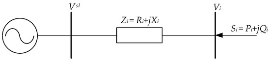
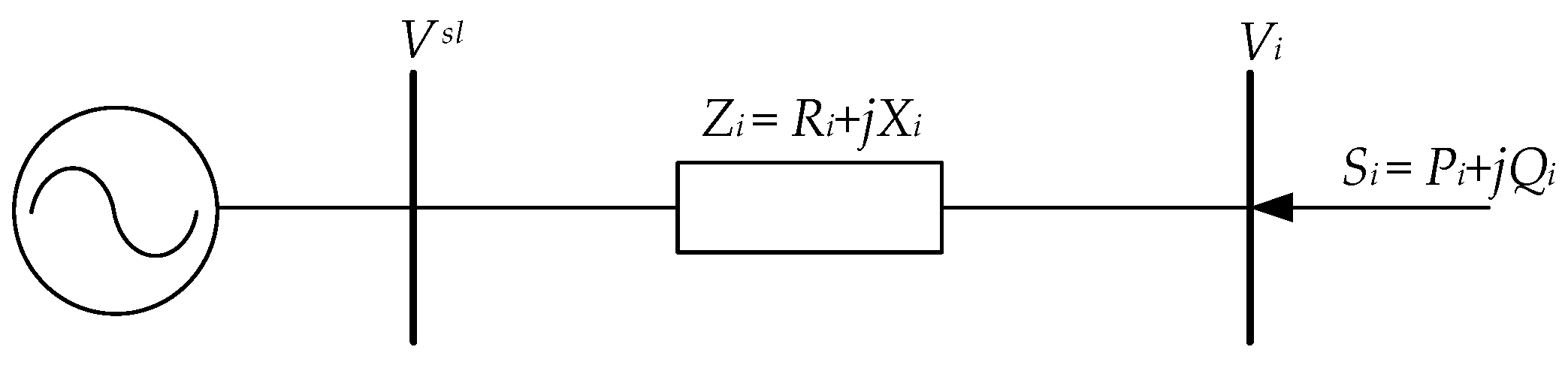
Referring to Ref. [27], the distribution network is decoupled by establishing two-bus virtual channels between each bus and the balancing bus, as illustrated in Figure 1.
Figure 1.
Two-bus virtual channel.
The power flow in the two-bus virtual channel is expressed by Equation (2):
where Zi is the impedance of the virtual channel; Si is the complex power injected at bus i; Vi is the voltage at bus i; and Vsl is the balancing bus voltage.
Based on Equation (2), introduce the normalised voltage Ui = Vi/Vsl and rearrange it as follows:
where μi is the complex-valued voltage stability index, expressed as follows:
Equation (3) is essentially a quadratic equation in one variable and can be solved using the quadratic formula:
where
In the formula, μR and μI are the real and imaginary parts of the voltage index.
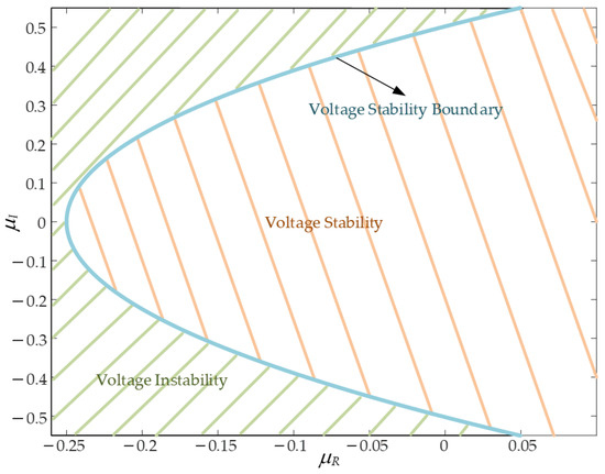
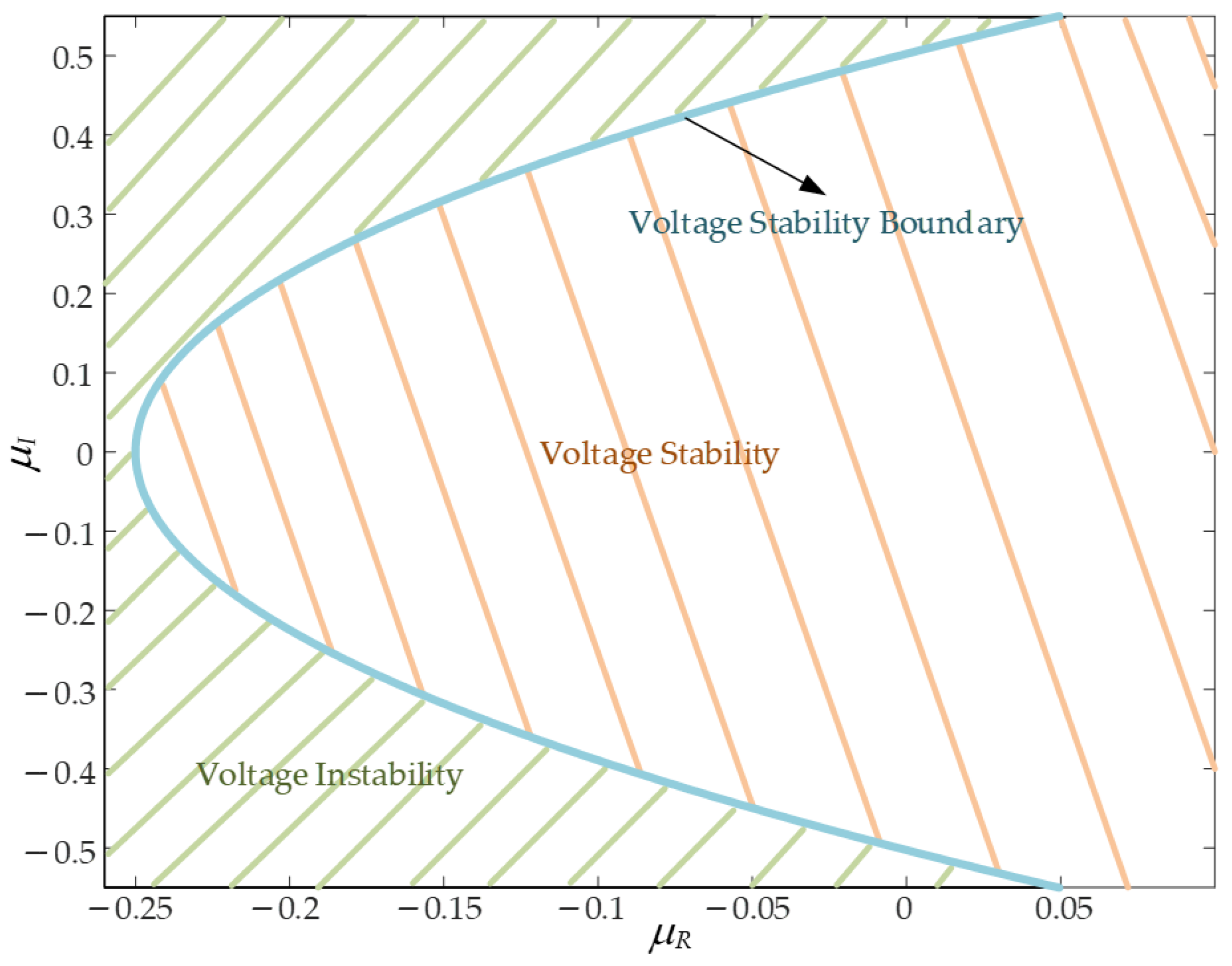
According to the criterion in Equation (6), a feasible solution set for the normalised bus voltage Ui in Equation (3) exists if and only if Δ > 0. In this case, the corresponding voltage index μi lies within the parabola defined by μR and μI. When Δ < 0, voltage collapse occurs, and μi exceeds the voltage stability boundary of the parabola. The critical condition Δ = 0 represents the voltage stability limit. This indicates that the system operating point has reached the saddle-node bifurcation threshold, with μi located on the parabola boundary. The voltage stability parabola of μi in the complex plane is illustrated in Figure 2.
Figure 2.
Parabolic boundary of voltage stability formed by μi in the complex plane.
By introducing the holomorphic embedding factor α, which represents the load level, Equation (3) can be reformulated as follows:
Moving μi(α) to the left-hand side of the equation:
Expanding Equation (8) into a Maclaurin series and equating the coefficients of the power series on both sides of the equation:
The analytical expression for the physical trajectory of the voltage stability index is as follows:
Once the analytical expression of the physical trajectory of the voltage stability index μi(α) with respect to the system load is obtained, the intersection points between μi(α) for all buses and the corresponding voltage stability parabola boundaries can be determined by simultaneously solving Equations (A10) and (9):
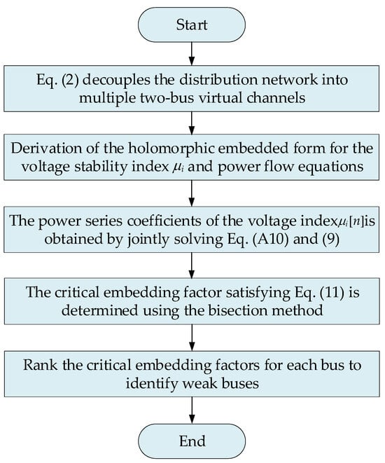
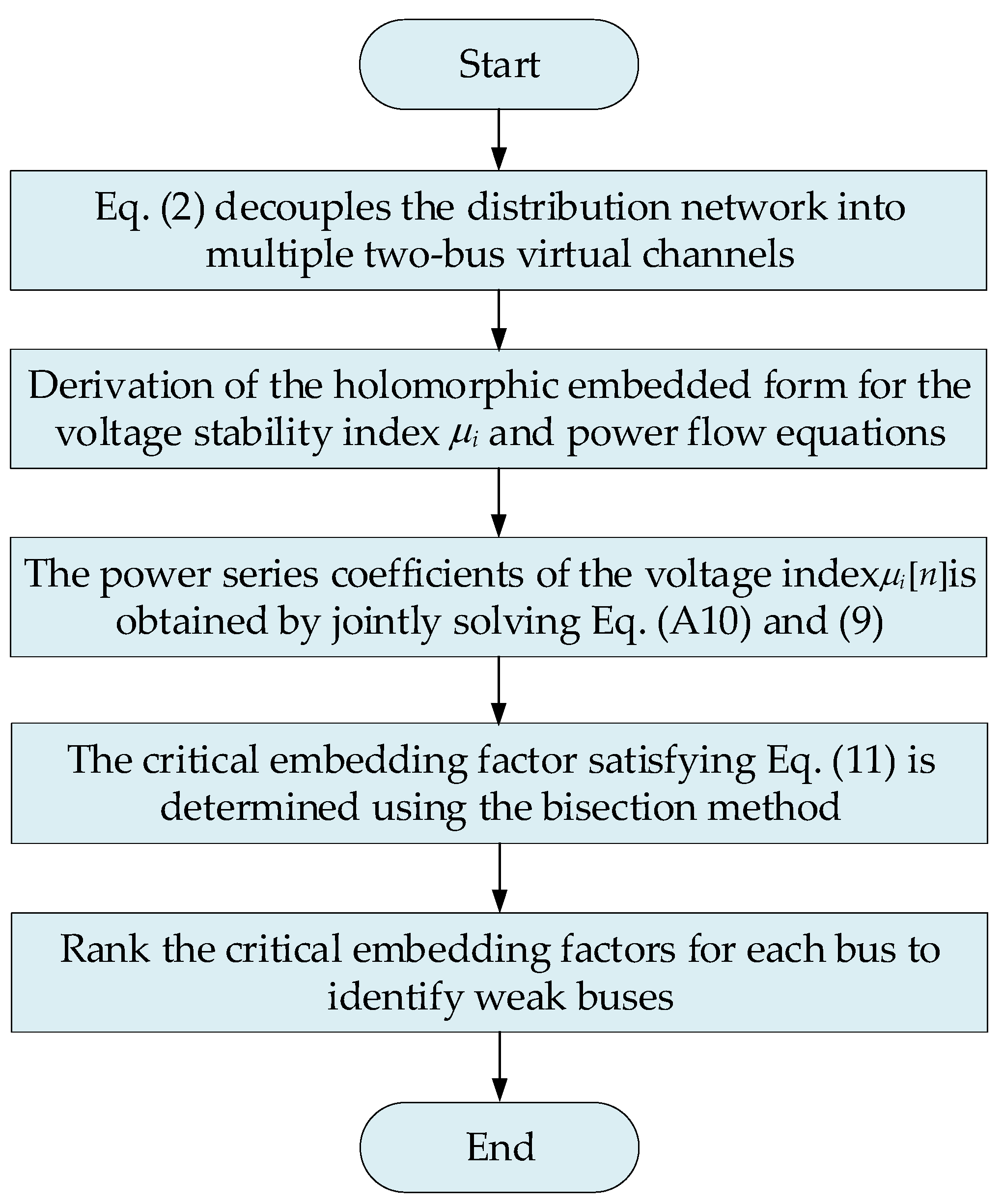
Equation (11) is a higher-order univariate equation with respect to α. To obtain its minimum positive real root, the bisection method is applied to solve for the smallest positive real root that satisfies Equation (11) [28], which corresponds to the critical embedding factor α. By comparing the values of α for all buses, their voltage weakness levels can be ranked. A smaller α value indicates that voltage collapse may occur under a smaller load increase. This implies poorer voltage stability and a higher instability risk for the corresponding bus. The procedure for identifying weak buses based on holomorphic embedding is illustrated in Figure 3.
Figure 3.
Flowchart of voltage weak buses identification.
3. Bi-Level UPQC Optimal Configuration Model
3.1. Bi-Level Optimal Configuration Model
Research on an optimal UPQC configuration method that integrates planning and operation aims to achieve effective voltage regulation while minimising operational costs. The bi-level optimal configuration model proposed in this paper incorporates dynamic voltage regulation strategies for the UPQC and is described as follows.
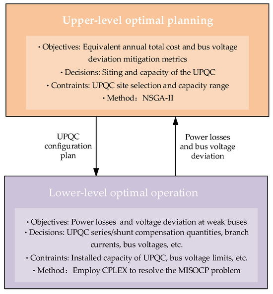
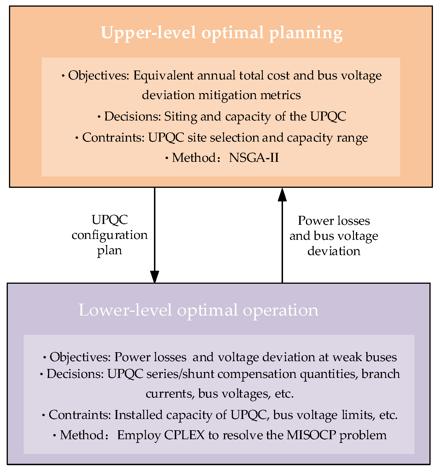
The upper level optimisation model adopts a multi-objective formulation. It minimises the equivalent annual total cost and bus voltage deviation metrics. The NSGA-II algorithm is used to determine the siting and capacity of the UPQC. The resulting configuration is then imposed as constraints on the lower level model. In the lower level model, based on the weak bus identification results in Section 2.2, the objective is to minimise voltage deviation and power losses over a typical day. The corresponding MISOCP problem is solved to obtain the optimal dispatch scheme under the dynamic voltage regulation strategy of the UPQC. The power losses and bus voltage deviations obtained at the lower level are fed back into the upper level objective function for evaluation. This enables the calculation of the equivalent annual total cost and voltage deviation mitigation metrics for the UPQC configuration scheme. The typical day scenario is modelled with an hourly resolution to capture the dynamic behaviour of load and DG output. The planning and operational levels are tightly coupled through this interaction, resulting in an optimised UPQC configuration that jointly considers the operational cost and voltage quality. The overall framework of the bi-level UPQC optimal configuration is illustrated in Figure 4.
Figure 4.
The framework for bi-level optimal configuration of UPQC.
3.2. Upper-Level Optimal Planning Model
The upper level optimisation establishes a multi-objective optimal planning model, minimising both the equivalent annual total cost and bus voltage deviation metrics. Given a fixed number of UPQCs to be installed, it determines the optimal siting and capacity allocation for these units.
3.2.1. Objective 1: Equivalent Annual Total Cost of Configuration Scheme C1
The total equivalent annual cost C1 of the UPQC configuration scheme comprises the equivalent annual investment cost CINV of equipment, the annual operation and maintenance cost COM, the decommissioning and disposal cost CDDC, and the distribution network operation cost CL. The relevant objective function may be expressed as follows [29]:
where,
In the formula, ICRF is the equivalent annual conversion coefficient for UPQC; nUPQC is the number of UPQCs installed; CUPQC is the installation cost per unit capacity of UPQC; is the installed capacity of the i-th UPQC; CLA, CT, and CE denote the labour costs for routine equipment maintenance, periodic testing costs, and fault repair costs, respectively; b and c are the residual value of scrapped assets and the proportion of disposal management costs relative to the initial investment, respectively, taken as 2% and 5% in this paper; r and T are the discount rate and service life of the UPQC; PLoss is the total power losses for a typical daily scenario; PG is the active power output of the generator; and λe and h are the electricity price and annual equivalent continuous operating days, respectively.
3.2.2. Objective 2: Bus Voltage Deviation Mitigation Metrics C2
To evaluate the effectiveness of bus voltage deviation mitigation, voltage deviation is defined as follows:
where ΔVi,t and Vi,t denote the voltage deviation and voltage magnitude of bus i at time t, respectively; ΔVi and Vi denote the corresponding voltage deviation and voltage magnitude of bus i without optimised configuration; and Vexp is the expected voltage value, taken as 1.0 p.u.
The bus voltage deviation mitigation metric is expressed as follows:
where cu is the penalty term per unit voltage deviation, with cu set at 1000 CNY/p.u. in this paper, and N is the total number of distribute network buses.
3.2.3. Constraints of the Upper Level Model
The upper level optimal planning model must satisfy constraints regarding the installed capacity, installation siting, and number of installations for the UPQC:
where is the installation siting of the i-th UPQC; Nbc represents the set of candidate installation buses for the UPQC; and QUPQC max is the upper-limit of the permissible installation capacity for the UPQC.
3.3. Lower Level Optimised Operational Model
The lower level optimisation formulates an operational model aimed at minimising power losses and voltage deviations at weak buses. Based on decision variables such as the series–shunt compensation settings of UPQC units under typical daily scenarios, the model determines the optimal dispatch scheme that satisfies both economic and operational safety requirements.
3.3.1. Objective: Power Losses and Voltage Deviations at Weak Buses
The lower level optimal operation aims to minimise power losses and voltage deviations at weak buses. To facilitate solution, both objectives are assigned identical weighting coefficients and are linearly combined into a single objective function:
where
In the formula, PLoss0,t and PLoss,t are the power losses before and after optimisation in the t-th time period, respectively; 24M is the size of the set Nim, which comprises the M weakest buses ranked by the weak index at each time period in a typical daily scenario, and M is set to five in this paper. The value of M is selected based on practical planning considerations to maintain focused voltage regulation and avoid overly dispersed control actions. Fi denotes the frequency with which the i-th weak bus appears in the set of weak buses; and are the squares of the weak bus voltages before and after optimisation, respectively; and are the deviations in the squares of the weak bus voltages before and after optimisation; i and j are the endpoint numbers of branch l; Bl is the set of branches; Nl denotes the set of branch endpoints; Iij,t denotes the branch current during the t-th time period; and rij denotes the branch resistance.
3.3.2. Constraints of the Lower Level Model
The optimal power flow model based on branch power flows is transformed into a MISOCP problem [30] and, combined with the dynamic voltage regulation strategy of the UPQC, the constraints for the lower level model can be established.
- (1)
- Equality constraints.
Let and ; the equality constraints may be expressed as follows:
where p and q are the active and reactive power injected at the bus; Pij and Qij are the active and reactive power of the branch; xij, gj, and bj denote the reactance, conductance, and admittance of the branch; N is the total number of buses; δ(j) is the set of terminal buses of branches originating from bus j; π(j) is the set of initial buses of branches terminating at bus j; Pload/Qload, PG/QG, Ppv/Qpv, and Pwind/Qwind are the active/reactive power outputs from loads, generators, photovoltaics, and wind turbines, respectively; and QUPQC,j represents the compensation quantity of the UPQC.
- (2)
- Inequality constraints.
Equation (22) represents the application of SOCR to the branch current equality constraints within the original branch power flow equations; Equations (23)–(25) define the upper and lower bounds for generator output, branch currents, and bus voltages, respectively.
3.3.3. UPQC Modelling
The UPQC adopts a back-to-back converter topology. The series converter is connected to the grid through a coupling transformer, while the shunt converter is directly connected to the bus. The device dynamically injects a compensating voltage via the series unit to correct line voltage drops. At the same time, the shunt unit regulates the injected reactive power at the bus to stabilise the voltage magnitude. The UPQC also integrates functions such as dynamic reactive power compensation and harmonic suppression. Together, these functions form a comprehensive control capability that addresses both voltage regulation requirements under DG integration and inherent grid power quality issues [31]. In developing the mathematical model of the UPQC, particular emphasis is placed on its dynamic voltage regulation strategy. The series compensation module is modelled as an on-load tap-changing transformer with dynamic regulation characteristics. This allows precise bus voltage control through real-time adjustment of the equivalent tap position. The shunt compensation module is represented using the dynamic model of an SVG, enabling continuous and smooth reactive power compensation [32]. This equivalent modelling approach, based on functional decoupling, effectively captures the coordinated interaction between the series and shunt compensation modules of the UPQC during dynamic voltage regulation.
- (1)
- Constraints for series compensation module.
The serial dynamic voltage compensation module must account for multi-period constraints, primarily encompassing adjacent adjustment increment limits, adjustment frequency limits, tap change indicator restrictions, voltage regulation range limitations, and transformation ratio range restrictions, as detailed below:
where is a 0–1 identifier storing the gear position information for the t-th time period; is a 0–1 identifier storing the gear increment/decrement information for the t-th time period; SRj denotes the maximum tap position; NUPQC represents the set of buses connected to the UPQC; indicates the maximum number of adjustable steps for the series compensation module, set to 10 in this paper; is the internal voltage value of the series compensation module, set to 1.0 p.u. in this paper; rj,t is the square of the adjustable ratio; and is the upper and lower limits of the adjustable ratio square.
At this point, the voltage squared at the UPQC access bus can be expressed as follows:
where rj,s is the adjustment increment between adjacent steps.
- (2)
- Constraints for shunt compensation module.
The UPQC shunt reactive power compensation module is represented as follows:
where and are the upper/lower limit of the UPQC’s shunt reactive power compensation capacity. Let to address bidirectional voltage overlimit issues in active distribution networks, and equals the installed capacity of the UPQC; is the shunt reactive power compensation capacity of the UPQC at the t-th time period.
3.3.4. Solution Method for Bi-Level Optimisation Models
The upper level planning model is formulated as a multi-objective optimisation problem, with objectives including the equivalent annual total cost of the UPQC configuration scheme and the effectiveness of voltage deviation mitigation. As these objectives are inherently conflicting, a set of compromise solutions is obtained through a global search process. Accordingly, the NSGA-II algorithm, which is well-known for its strong multi-objective search capability [33], is adopted to determine the optimal UPQC configuration schemes.
The lower level operational problem involves two performance metrics: total system power losses and voltage deviation at weak buses. In the bi-level framework, the upper level planning problem is solved using NSGA-II without assigning explicit weights to the objectives. In contrast, the lower level operational optimisation adopts a linear weighted-sum formulation with equal weights for power loss and voltage deviation. This setting avoids imposing an a priori preference on either objective during the operational optimisation process and is consistent with common practices in existing bi-level optimisation studies [34,35]. Owing to the highly constrained and nonlinear nature of the lower level model, the SOCR method is applied to linearise the problem, thereby improving the computational efficiency of solving the lower level operational optimisation model.
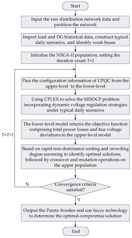
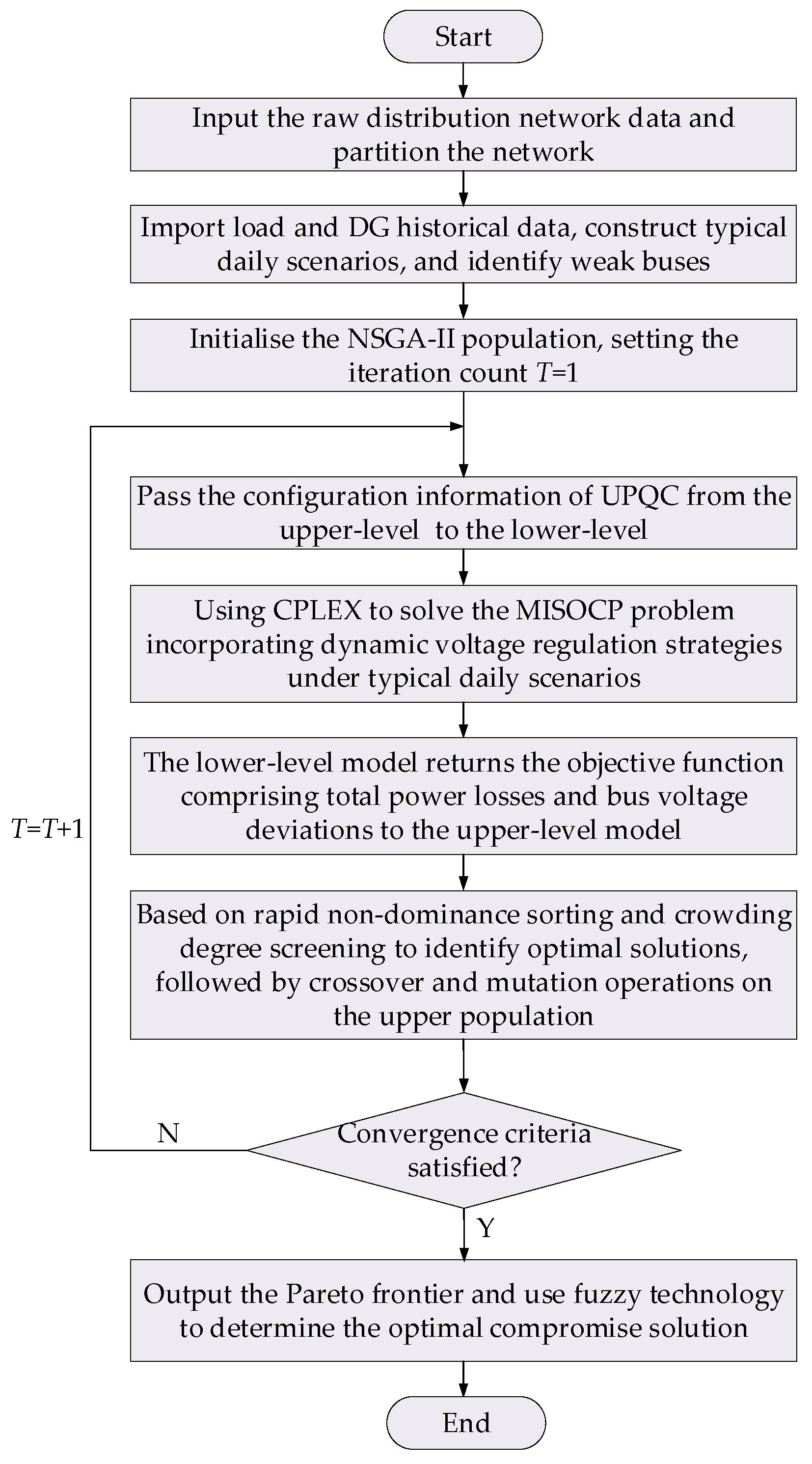
In the bi-level model, the upper level generates UPQC configuration schemes according to the optimisation objectives, and the resulting configurations are transmitted to the lower level as constraints. The lower level then computes the optimal operational scheme for typical daily scenarios under these constraints. The total system power losses and bus voltage deviations are fed back to the upper level objective function. During the solution process, the upper level applies the NSGA-II algorithm, while the lower level uses the CPLEX solver to solve the MISOCP problem. The two levels are optimised alternately until the convergence criterion is satisfied. Specifically, the process terminates when the difference between two consecutive iterations is less than 10−5 or when the maximum number of iterations is reached. The proposed model ultimately produces a Pareto frontier that balances the operational cost and voltage stability. Fuzzy decision-making technology [20] (see Appendix A.3 for details) is then employed to select the optimal compromise solution from the set of non-dominated solutions. The overall solution procedure of the bi-level optimal configuration model is illustrated in Figure 5.
Figure 5.
Solution process of the bi-level optimal configuration model.
4. Case Study
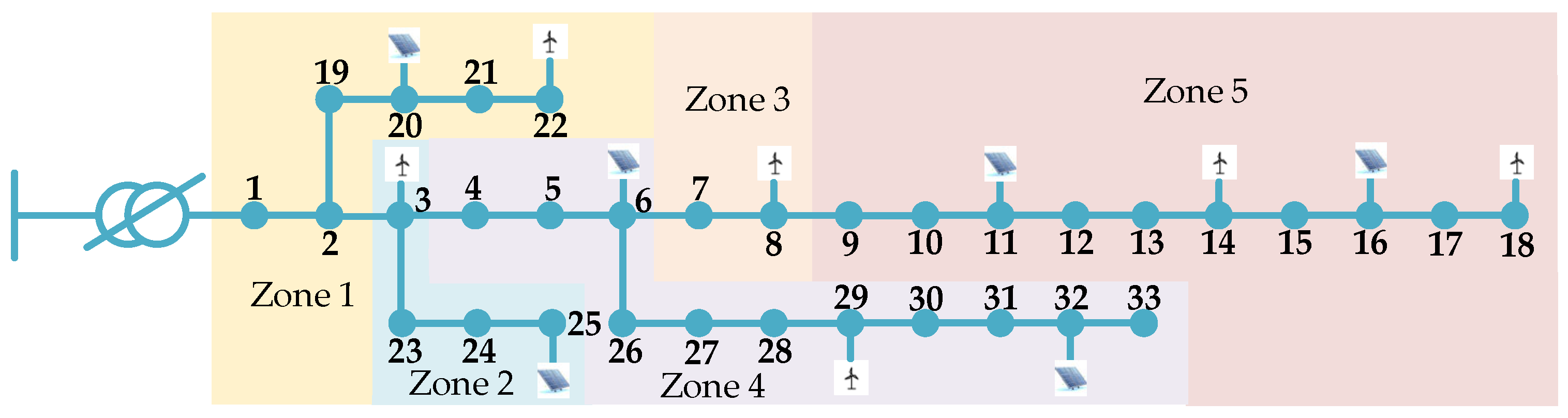
This paper demonstrates the effectiveness of the proposed UPQC optimal configuration method by using an extended IEEE-33 bus power system and real-world distribution networks (see Appendix B for details). The system operates at a reference voltage of 10 kV and a reference power of 10 MVA. While retaining the standard system topology and parameters, distributed photovoltaics with a capacity of 0.8 MW are deployed at buses 6, 11, 16, 20, 25, and 32, and wind turbines with a capacity of 0.5 MW are installed at buses 3, 8, 14, 18, 22, and 29. All DGs operate at a power factor of 0.8.
Furthermore, the original load curve is modified based on actual load fluctuation characteristics to simulate scenarios with high DG penetration. The number of UPQCs installed is set to one. The permissible installation capacity range of the shunt compensation module of a single UPQC is 0–5 MVar, while the voltage regulation range of the series compensation module is 0.95–1.05 p.u. The service life of the UPQC is assumed to be 20 years, with an installation cost of 400,000 CNY/MVar and a discount rate of 0.05. The annual maintenance cost is 7500 CNY per unit, the electricity tariff is 0.5 CNY/kWh, the number of equivalent operating days per year is 365, and the allowable bus voltage range is 0.95–1.05 p.u.
The upper level optimisation is performed using the NSGA-II algorithm, with a population size of 100, a maximum of 50 generations, and both crossover and mutation probabilities set to 0.8. The lower level optimisation is solved using the YALMIP/CPLEX solver, with the solution tolerance set to 10−4.
All computations are performed on a personal computer equipped with an Intel Core i5-9300H processor (2.40 GHz) and 32 GB of memory, using MATLAB R2022a.
4.1. Network Partitioning and Weak Bus Identification
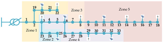
Based on the reactive power–voltage sensitivity partitioning method described in Section 2.1, the active distribution network can be divided into five zones. Zone 5 exhibits the highest reactive power–voltage sensitivity, followed by Zone 4, while Zone 1 exhibits the lowest sensitivity. The partition sensitivity metrics are presented in Table 1, and the extended IEEE-33 bus power system is illustrated in Figure 6.
Table 1.
Partition sensitivity index of the extend IEEE-33 bus power system.
Figure 6.
Extended IEEE-33 bus power system.
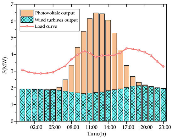
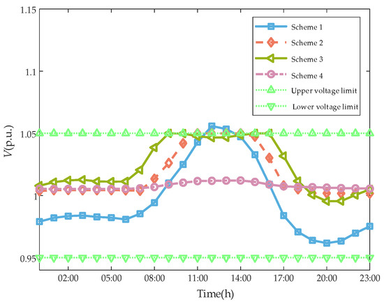
Based on actual load measurements and historical DG data from a specific region, representative daily source–load variation characteristics were extracted to construct typical output scenarios. First, load and DG measurement data with a 15 min resolution were collected over an entire year and subjected to data cleansing and statistical analysis. Subsequently, a time-aligned averaging method was employed to calculate point-by-point averages of the 15 min data at identical times across the year, directly generating a typical daily curve reflecting the overall annual operational pattern. This method avoids clustering, filtering, or deliberate exclusion of data points. Consequently, adverse operating conditions—such as peak loads and low DG outputs—are preserved as natural components of the historical dataset. Their statistical characteristics remain intact within the typical day curve, ensuring that the constructed scenarios encompass all plausible extreme conditions. Furthermore, averaging the annual data prevents any single extreme day from dominating the configuration outcome. This approach safeguards voltage regulation effectiveness while avoiding overly conservative configurations that could incur unnecessary investment costs. The resulting typical daily output curves for the extended IEEE-33 bus power system are presented as stacked bar charts in Figure 7, and the corresponding numerical data are provided in Table A5.
Figure 7.
Curve of load and DG output in a typical day scenario.
As shown in Figure 7, during the period from 09:00 to 16:00, the total output of DG consistently exceeds the load power, resulting in reverse power flow within the distribution network. Due to the influence of line impedance characteristics, this reverse power flow will cause voltage uplift at the DG connection bus and adjacent buses, posing a risk of voltage exceeding the upper limit.
Based on the classical holomorphic embedding method for weak bus identification proposed in Section 2.2, the weak buses for each hour within a typical day were analysed sequentially, according to the workflow shown in Figure 3. For each hour’s DG and load data, holomorphic embedding power flow calculations were performed, yielding a ranking of bus weakness for that specific time period. The top five buses from each hourly ranking were recorded. After completing the analysis for all 24 h, the recorded buses were aggregated. The frequency of occurrence for each bus across the 24 periods was then statistically determined, forming the final set of key weak buses used to evaluate voltage control effectiveness during typical day operations. The identification results are presented in Table 2.
Table 2.
Weak bus identification results of the extend IEEE-33 bus power system.
4.2. Validation of the Effectiveness of Reactive Power Configuration Schemes
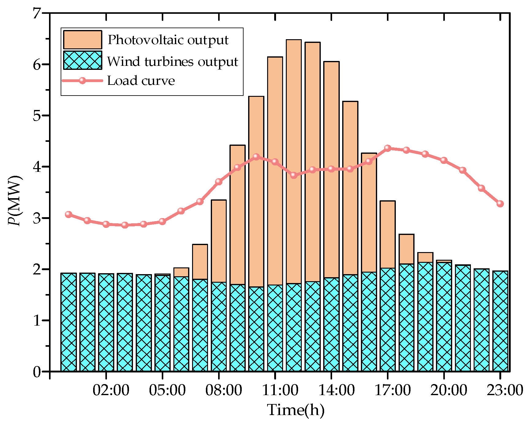
To validate the effectiveness of the proposed UPQC series-shunt coordinated voltage regulation strategy in enhancing voltage quality within active distribution networks, this study compares three implementation schemes. Scheme 1: No UPQC installation; Scheme 2: shunt compensation module only; Scheme 3: series compensation module only; and Scheme 4: concurrent deployment of both series and shunt compensation modules (UPQC installation). The candidate installation zone is Zone 5. In this comparison, the voltage deviation metric is calculated as the sum, over a 24 h typical day, of the absolute difference between each bus voltage and the slack bus reference voltage. The optimised configuration results for each scheme are presented in Table 3.
Table 3.
Comparison of reactive power optimised configuration results.
Table 3 indicates that although Scheme 2 and Scheme 4 share identical UPQC installation capacities, their differing installation locations and compensation modes yield distinct mitigation effects. The configuration of Scheme 2, positioned closer to the main grid, primarily reduces reactive power flow across the entire network. Consequently, it achieves a 35.43% reduction in power losses compared to Scheme 1. Scheme 4, situated nearer the end of the distribution network, focuses more on precise local voltage regulation. This results in a more pronounced improvement in voltage deviation, achieving a 48.46% reduction compared to Scheme 1. In contrast, Scheme 3 considers only series compensation. Although it provides a certain degree of voltage support, its overall performance is inferior to that of the full UPQC schemes. Compared with Scheme 1, Scheme 3 reduces power losses and voltage deviation by 24.80% and 15.84%, respectively, but its improvement remains limited due to the absence of shunt compensation. This outcome exemplifies the typical “power loss versus voltage” trade-off in reactive power and voltage management and provides clear decision-making guidance for planners prioritising either power loss reduction or voltage quality enhancement according to the operational objectives, with clear practical engineering significance.
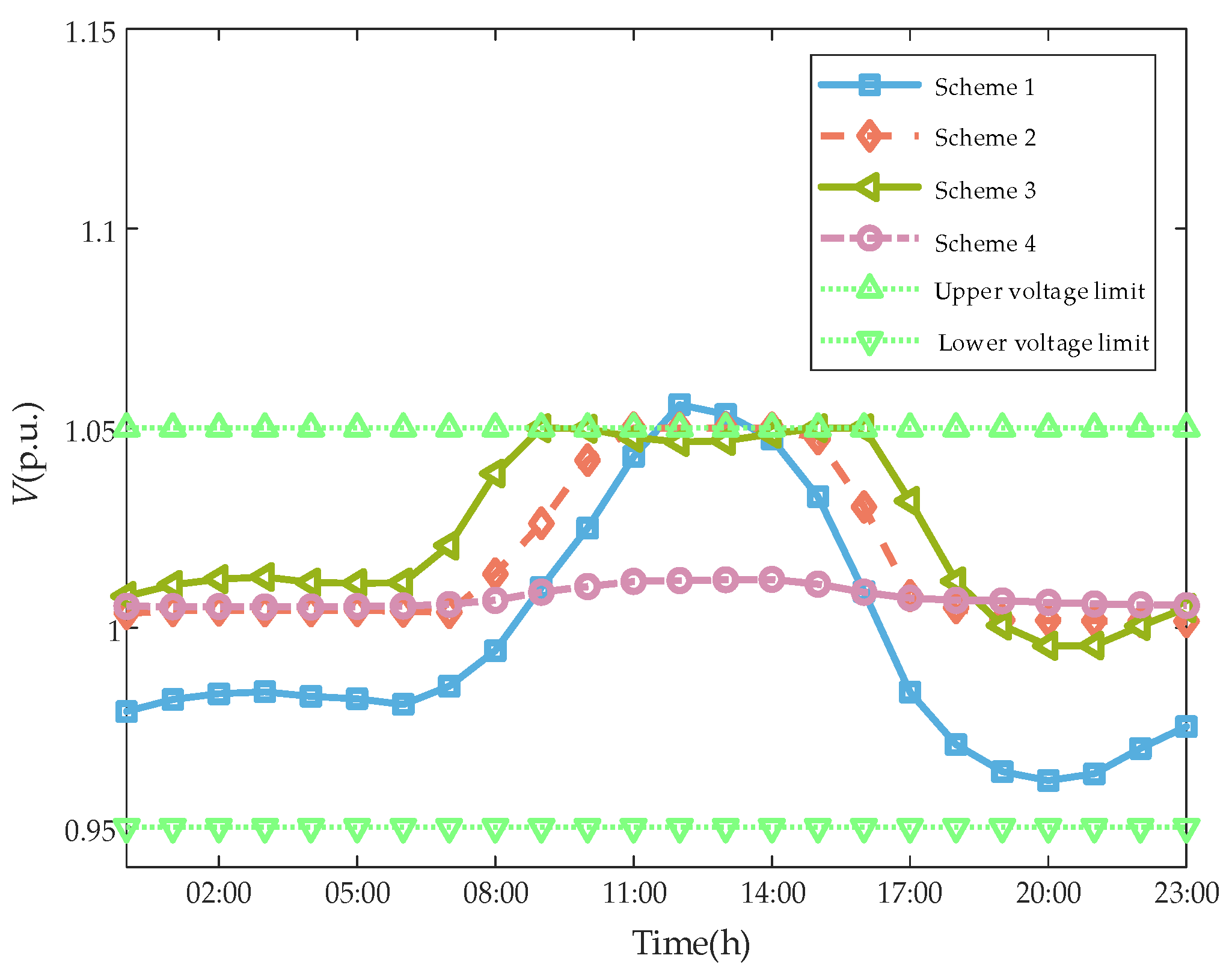
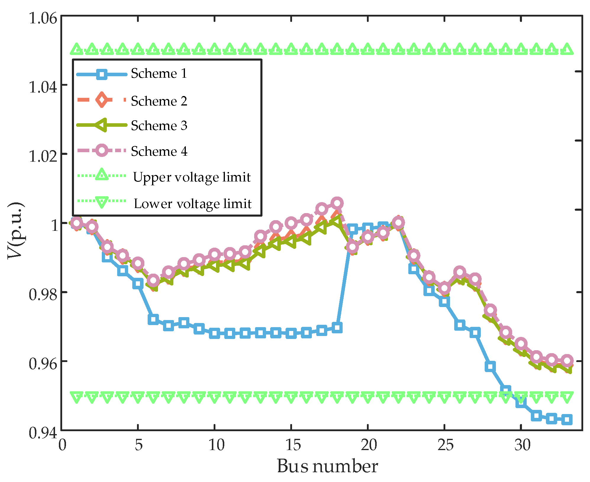
This paper focuses on mitigating bidirectional voltage violation issues caused by the integration of DGs into the grid, placing greater emphasis on enhancing voltage quality in distribution networks. Figure 8 further compares the voltages at terminal buses under different reactive power optimisation schemes to analyse the voltage regulation effectiveness of each approach.
Figure 8.
Voltage variation curve of Bus 18 in a typical daily scenario.
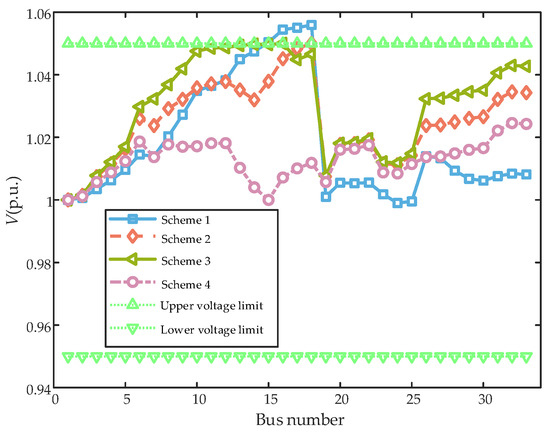
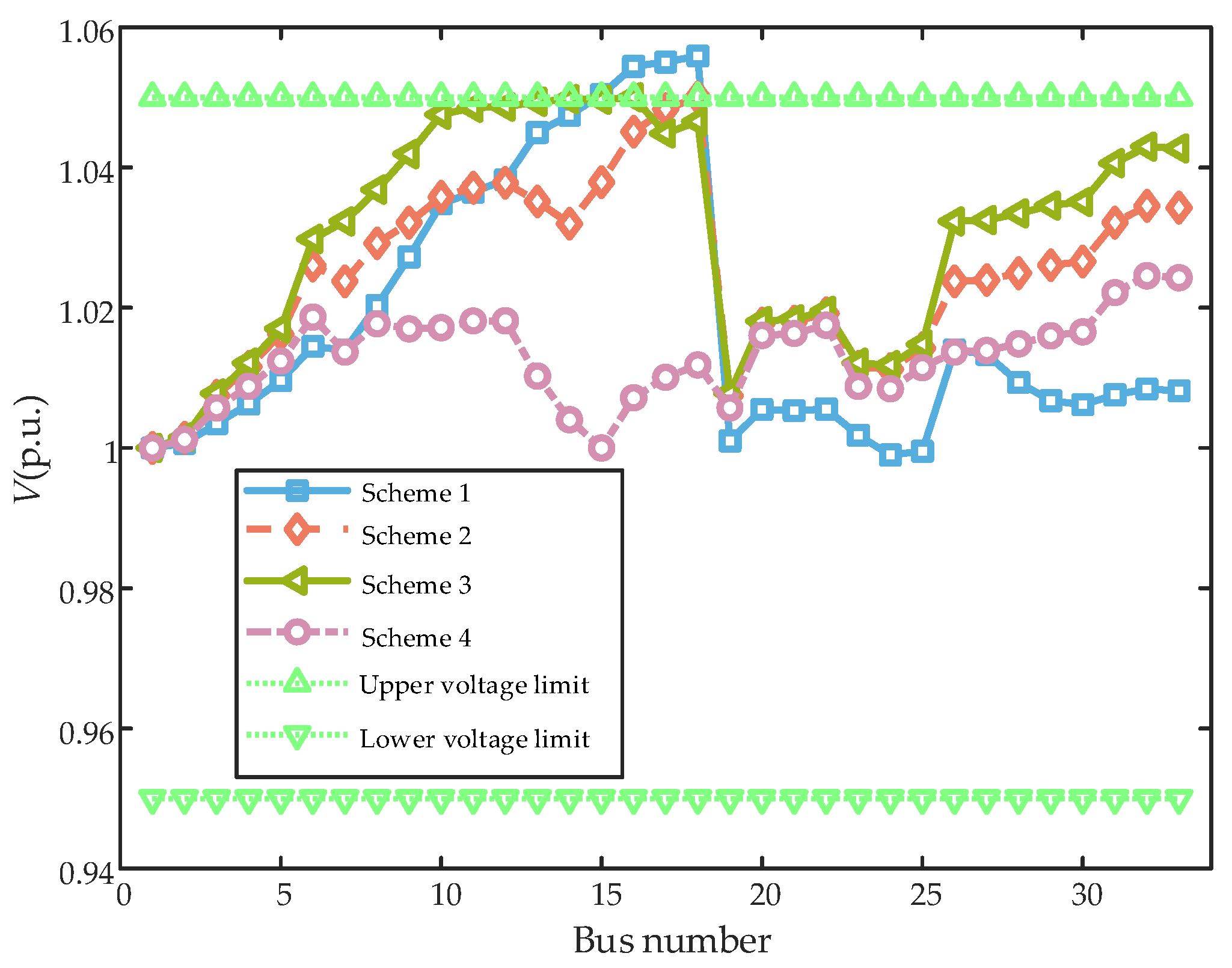
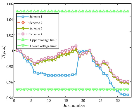
Figure 9 and Figure 10 illustrate voltage curves for different configuration schemes during two typical time periods. During the peak photovoltaic output period at 13:00, Scheme 4 achieved precise voltage control through the synergistic series-shunt compensation of the UPQC, effectively suppressing the voltage uplift caused by DG output backfeed. By contrast, Schemes 2 and 3, relying solely on shunt compensation modules during peak photovoltaic output, exhibit significant limitations in voltage control capability. Near buses 17 and 18, voltage persistently approaches the 1.05 p.u. limit, with an insufficient safety margin and substantial overall voltage deviation. During the low-load period at 22:00, Schemes 2, 3 and 4 effectively elevate voltage levels, mitigating the risk of voltage dips below the lower limit.
Figure 9.
Voltage curves under different reactive power compensation schemes at 13:00.
Figure 10.
Voltage curves under different reactive power compensation schemes at 22:00.
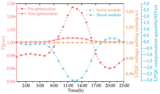
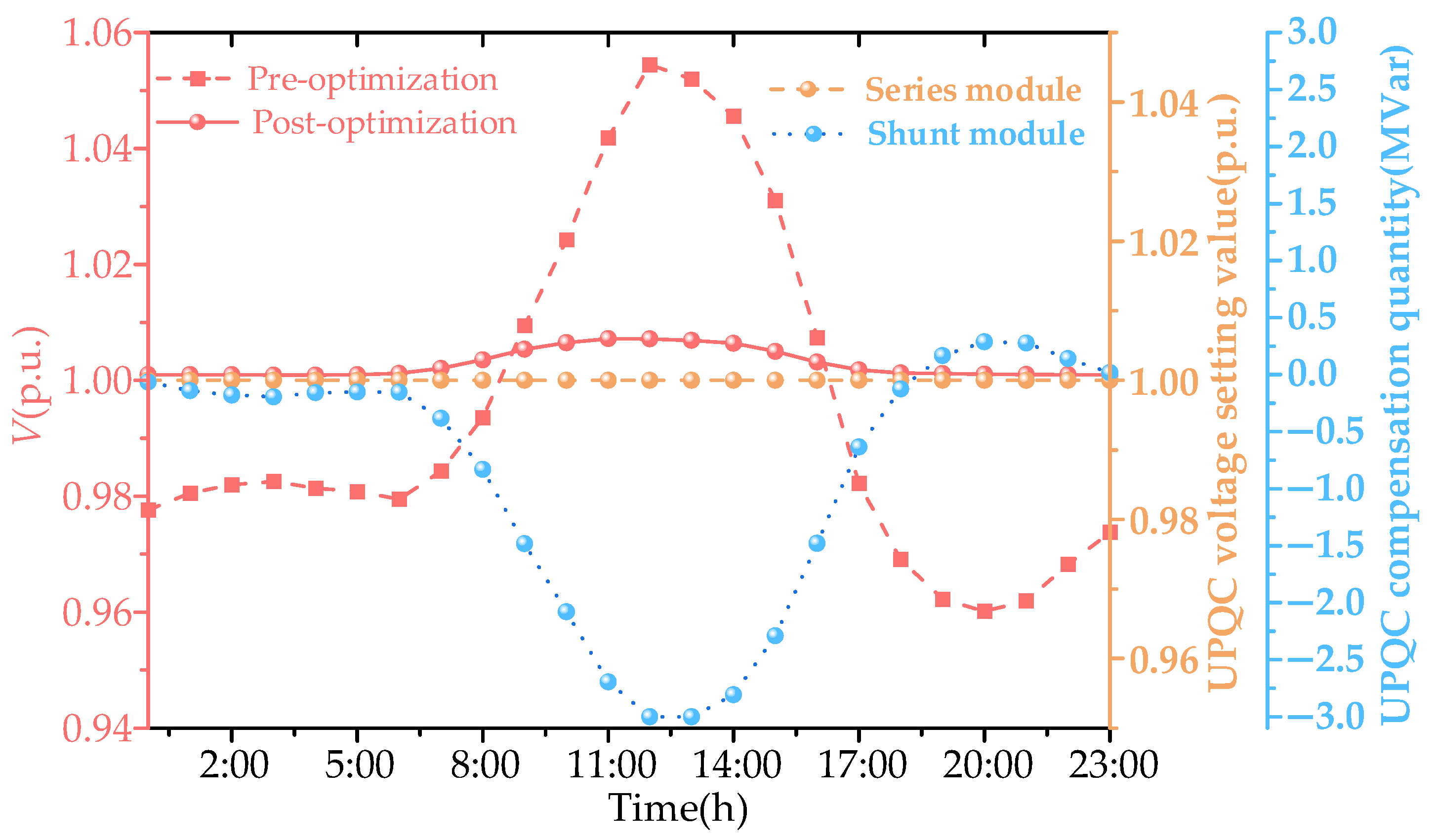
Taking the optimised configuration results of Scheme 4 as an example, this paper investigates the impact of the UPQC access Bus 15 on its adjacent Bus 16. Figure 11 illustrates the voltage fluctuation curve of Bus 16 before and after the UPQC optimisation, alongside the dynamic response of the UPQC’s series-shunt compensation modules.
Figure 11.
Dynamic voltage regulation operation status of UPQC.
Results indicate that the UPQC significantly mitigates voltage fluctuations. During peak photovoltaic output periods, the shunt compensation module dynamically adjusts to absorb the redundant reactive power from the grid, effectively suppressing voltage uplift at Bus 16. During night-time low-load periods, it dynamically releases reactive power to elevate voltage levels. The series compensation module, utilising an on-load tap-changing transformer with dynamic regulation capabilities, injected compensating voltage into the bus. This ensured that the voltage at the UPQC connection point remained consistently within the target deviation range. This dynamic voltage regulation strategy automatically adjusted reactive power injection and series voltage compensation, according to varying load and DG output conditions. It achieved sustained management of voltage deviations at weak buses, validating the rationality and effectiveness of the UPQC dynamic voltage regulation strategy.
4.3. Validation of the Bi-Level Optimisation Model
To validate the efficacy of the bi-level optimisation model, this paper conducts a comparative study with a single-level optimisation model. The following provides a brief introduction to the single-level optimisation model, comparing it with the bi-level optimisation model in terms of both the model itself and the solution methodology.
Regarding the models, the single-level optimisation model corresponds to the upper level within the bi-level optimisation model, while simultaneously incorporating the constraints associated with the operational characteristics of the UPQC from the lower level. This is specifically illustrated in Equations (12)–(16) and Equations (26)–(32).
Regarding the solution methodology, within the bi-level optimisation model, the decision variables for the NSGA-II algorithm encompass the siting and capacity of the UPQC. In contrast, the single-level optimisation model incorporates these decision variables while additionally introducing the selection of tap settings for the UPQC series compensation module. Beyond this distinction, both models employ identical methods for calculating power losses and bus voltage deviations in the case study. Furthermore, the parameter settings for the NSGA-II algorithm remain consistent across models, ensuring fairness and consistency in the comparative results.
The distribution network was optimally configured with UPQC using the following three models. Model 1: No UPQC configuration; Model 2: single-level optimised UPQC configuration; and Model 3: bi-level optimised UPQC configuration. The UPQC configuration results for each optimisation model are detailed in Table 4.
Table 4.
Comparison of optimal configuration results for different models.
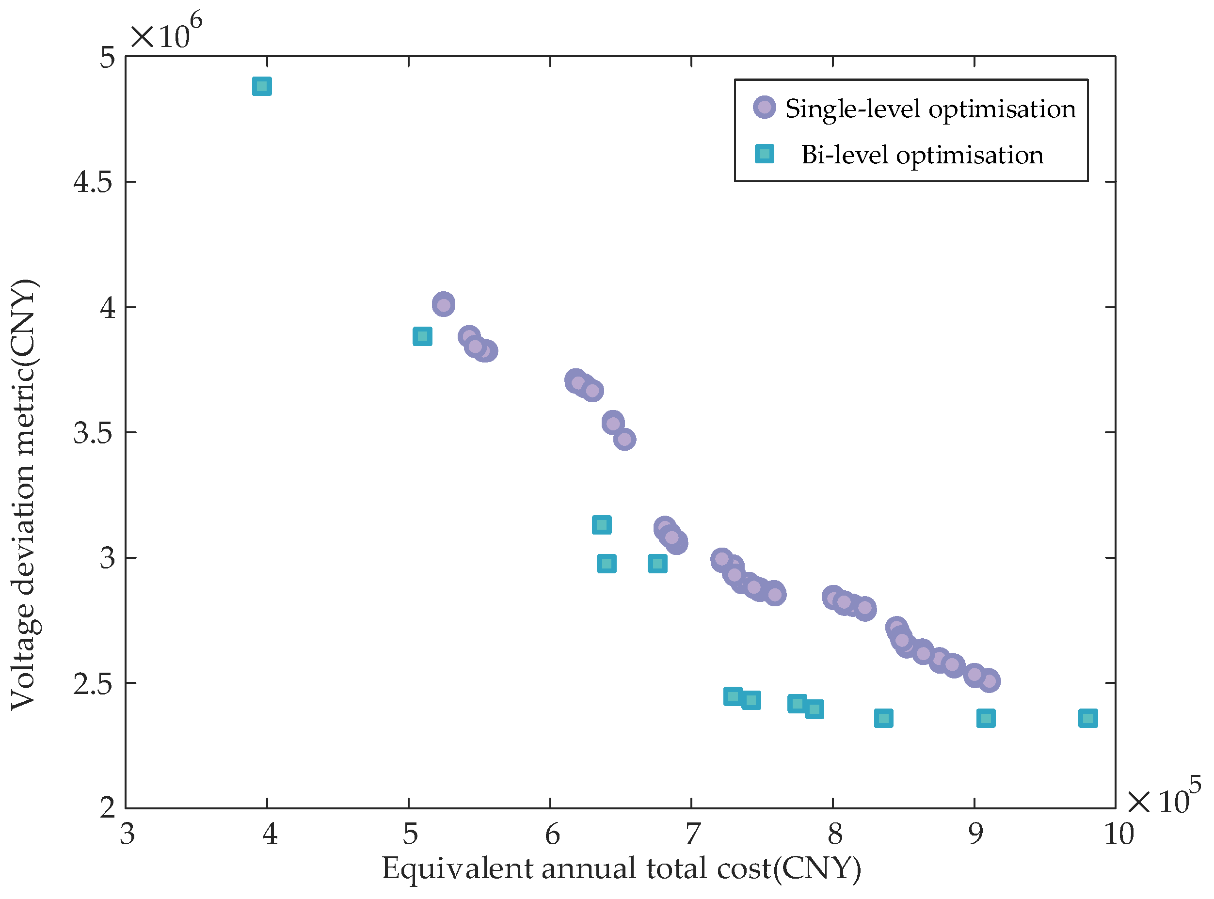
Model 2 reduced the power losses by 13.00% and bus voltage deviation by 41.97% compared to scenarios without UPQC reactive power compensation equipment. Building upon Model 2, Model 3 further decreased power losses by 1.81% and bus voltage deviation by 11.28%. This demonstrates that Model 3 outperforms Model 2 in reducing power losses and voltage deviation, particularly excelling in mitigating voltage deviation. Consequently, the effectiveness of the dual-layer optimisation model is validated.
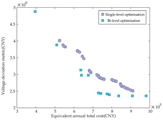
As shown in Figure 12, under identical parameter settings, the UPQC configuration scheme of the bi-level model outperforms the single-level model in both the total equivalent annual cost and voltage deviation metrics, exhibiting lower numerical values. Furthermore, the single-level model exhibits a greater number of scattered points compared to the bi-level model, indicating that the bi-level model converges earlier than its single-level counterpart. This further validates the effectiveness and superiority of the bi-level model. In addition, the well-distributed Pareto front, together with the observation that the number of non-dominated solutions stabilises well before the maximum number of NSGA-II generations, indicates that the algorithm achieves stable and consistent convergence.
Figure 12.
The Pareto frontiers of different models.
4.4. Impact of UPQC Connection Quantity on Distribution Network Planning Outcomes
In the preceding analysis, only a single UPQC was considered to clearly demonstrate the intrinsic voltage regulation capability of the device. To further investigate the impact of different numbers of UPQCs on distribution network voltage quality and operational costs, four comparative schemes were designed. By altering the number of UPQCs deployed (set to 0, 1, 2, and 3 units, respectively), simulations were conducted under typical daily scenarios for validation. The UPQC siting strategy adheres to the principle of ‘zonal independent compensation’: when configuring two units, the zones with the highest reactive power–voltage sensitivity (Zone 5) and the second-highest sensitivity (Zone 4) are selected. When configuring three units, an additional UPQC is deployed in the third-highest sensitivity zone (Zone 3). The optimised configuration results for different numbers of UPQCs are presented in the Table 5.
Table 5.
Configuration results for different UPQC connection quantities.
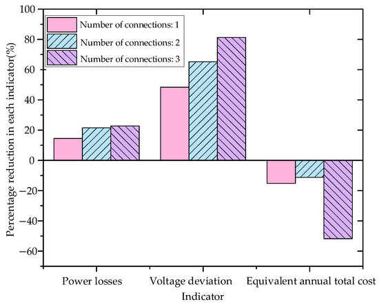
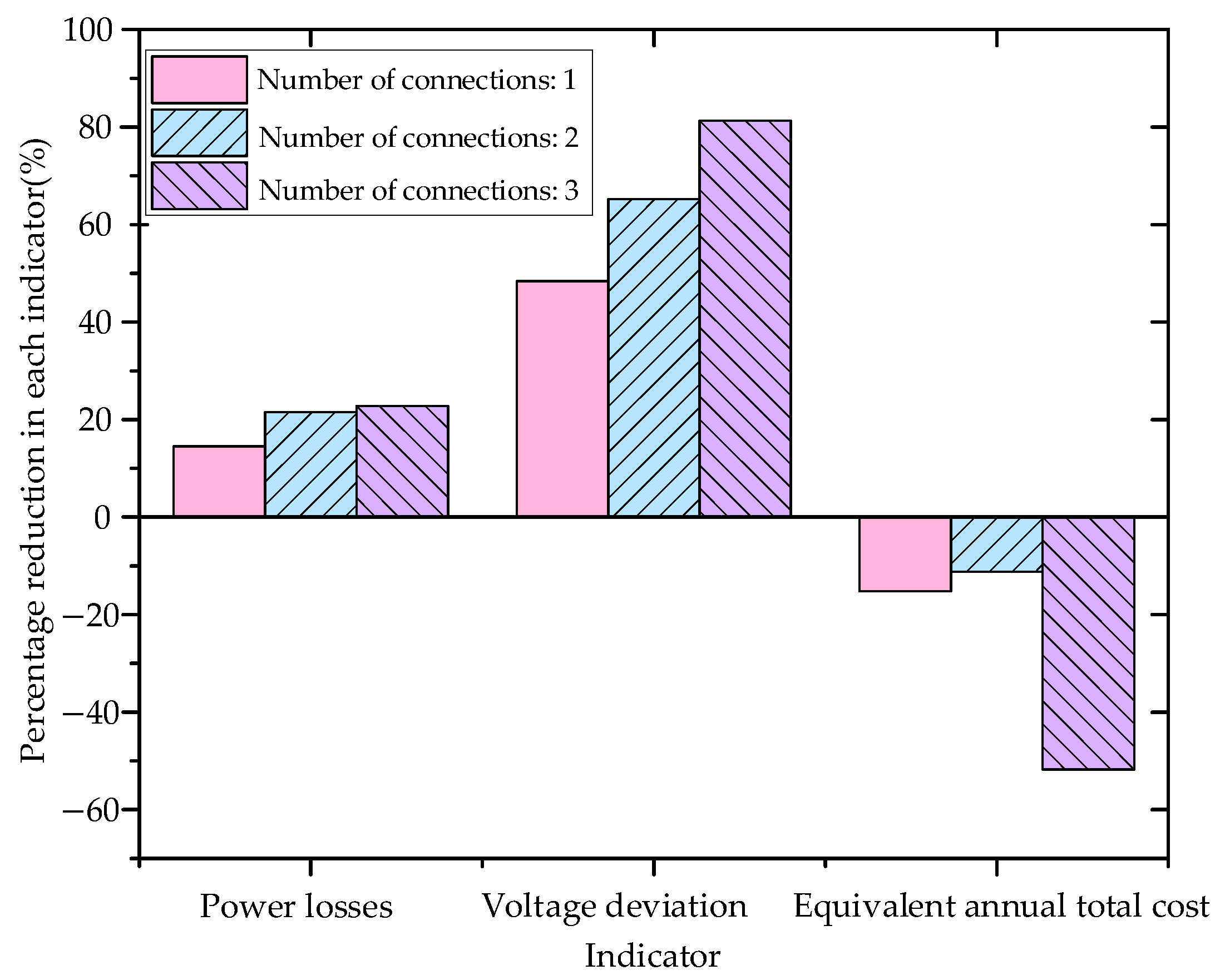
Using the planning scheme without UPQCs as the baseline for comparison, Figure 13 shows that both power losses and voltage deviations decrease gradually as the number of deployed UPQCs increases. This result confirms the effectiveness of UPQCs in improving the operational performance of distribution networks. Although the capital investment required for UPQCs is higher than the economic benefits gained from reduced power losses, the primary objective of this approach is to mitigate voltage over-limit problems caused by DG integration. This is achieved by optimising UPQC deployment to enhance the operational safety and stability of distribution networks.
Figure 13.
The impact of different numbers of UPQC accesses on distribution network planning.
In addition, the equivalent annual total cost exhibits a trend of first decreasing and then increasing as the number of UPQCs rises. During the initial deployment stage, a moderate increase in the number of UPQCs leads to a significant reduction in power losses, thereby lowering the equivalent annual total cost. However, once the number of UPQCs exceeds a critical level, further reductions in power losses become limited. As a result, the equivalent annual total cost increases sharply, due to the rising investment cost. Therefore, accurately identifying the critical configuration that minimises the incremental cost (such as the deployment of two UPQCs, as shown in Figure 13) is essential for improving the economic viability of the proposed configuration scheme.
5. Conclusions
To address voltage over-limit and under-limit issues caused by large-scale integration of DG into distribution networks, this paper proposes a bi-level optimal configuration method for the UPQC that integrates planning and operation. The proposed method is developed based on the dynamic voltage regulation strategy of the UPQC. Case studies validate the following conclusions:
(1) The proposed reactive power–voltage sensitivity-based partitioning method quantifies the coupling strength between buses and divides the distribution network into sub-regions with different sensitivity levels. This approach significantly narrows the candidate installation range for UPQC devices, thereby improving the accuracy and efficiency of site selection.
(2) The classical holomorphic embedding method is employed to identify voltage-weak buses, enabling accurate localisation of potential voltage instability areas. Voltage deviations at these weak buses are further used as key indicators for voltage quality management at the operational level. This strategy effectively enhances voltage stability in distribution networks.
(3) Compared with traditional single-level optimisation methods, the proposed bi-level optimisation framework integrates planning and operation. As a consequence, it achieves a better balance between operational security and overall network cost.
(4) By incorporating the dynamic voltage regulation strategy of the UPQC into the reactive power optimal configuration model, the proposed method effectively mitigates voltage over-limit and under-limit problems caused by high DG penetration. At the same time, system power losses are reduced.
Author Contributions
Conceptualisation, B.L. and Y.Z.; Methodology, B.L., X.W. and Y.Z.; Formal analysis, B.L., Y.H. and Z.Z.; Investigation, Y.H. and X.W.; Writing—original draft, B.L. and C.L. Visualisation, Y.Z.; Supervision, Y.Z. and C.L.; Writing—review and editing, Y.Z.; Project administration, Z.Z.; Funding acquisition, Z.Z. All authors have read and agreed to the published version of the manuscript.
Funding
This work was funded by the Science and Technology Project of State Grid Fujian Electric Power Co., Ltd. (No. 52136024000P).
Data Availability Statement
The raw data supporting the conclusions of this article will be made available by the authors upon request.
Conflicts of Interest
Authors Bin Lin, Yan Huang, and Xiangyu Wang were employed by the State Grid Longyan Power Supply Company of Fujian Electric Power Co., Ltd. Author Zhensong Zeng was employed by the Electric Power Research Institute, State Grid Fujian Electric Power Co., Ltd. The remaining authors declare that the research was conducted in the absence of any commercial or financial relationships that could be construed as a potential conflict of interest. The authors declare that this study received funding from the Science and Technology Project of State Grid Fujian Electric Power Co., Ltd. The funder was not involved in the study design, collection, analysis, interpretation of data, the writing of this article, or the decision to submit it for publication.
Abbreviations
The following abbreviations are used in this manuscript:
| UPQC | Unified power quality conditioner |
| DG | Distributed generation |
| MISOCP | Mixed-integer second-order cone programming |
| NSGA-II | Non-dominated sorting genetic algorithms |
| SVC | Static var compensator |
| SVG | Static var generator |
| SOCR | Second-order conic relaxation |
Appendix A
Appendix A.1. Jacobi Matrix Computation and Network Partitioning Diagram
For the i-th bus in the power system, the power balance equation is as follows:
where ΔPi, ΔQi, and Vi denote the active imbalance quantity, reactive imbalance quantity, and voltage magnitude at bus i, respectively; Gij, Bij, and θij represent the conductance, conductance matrix element, and voltage phase angle difference between buses i and j, respectively; Pi and Qi denote the active and reactive power injected at bus i, respectively; and n denotes the total number of buses in the system. All parameters except phase angle differences are normalised to unity.
The Linearising Equation (A2) yields the following:
where J denotes the Jacobian matrix of the power flow equations.
where H, N, M, and L denote the submatrices of J. For a distribution network comprising n buses (including one slack bus), the phase angle variables in the Jacobian matrix have a dimension of (n − 1), while the voltage magnitude variables correspond solely to the PQ buses. Let the number of PQ buses in the system be denoted as nPQ. The dimensions of the respective submatrices are then (n − 1) × (n − 1), (n − 1) × nPQ, nPQ × (n − 1), and nPQ × nPQ, respectively.
The expressions for the off-diagonal elements of each submatrix are as follows:
The expressions for the diagonal elements of each submatrix are as follows:
Following changes to the distribution network topology, the power flow calculation is first carried out under the new topology to determine the updated operated state of the system. Subsequently, the power flow Jacobian matrix is updated according to Equations (A4)–(A5), and a new reactive power–voltage sensitivity matrix is computed. As the Jacobian matrix excludes elements pertaining to slack bus, the slack bus is assigned to the partition with the closest electrical distance during the network partitioning process.
In Figure A1, the initial partition comprises four subpartitions: buses 1, 2, 3, and 4. The initial reactive-voltage modularity function is calculated using Equation (1).
Figure A1.
Schematic diagram of a four-bus power system partitioning.
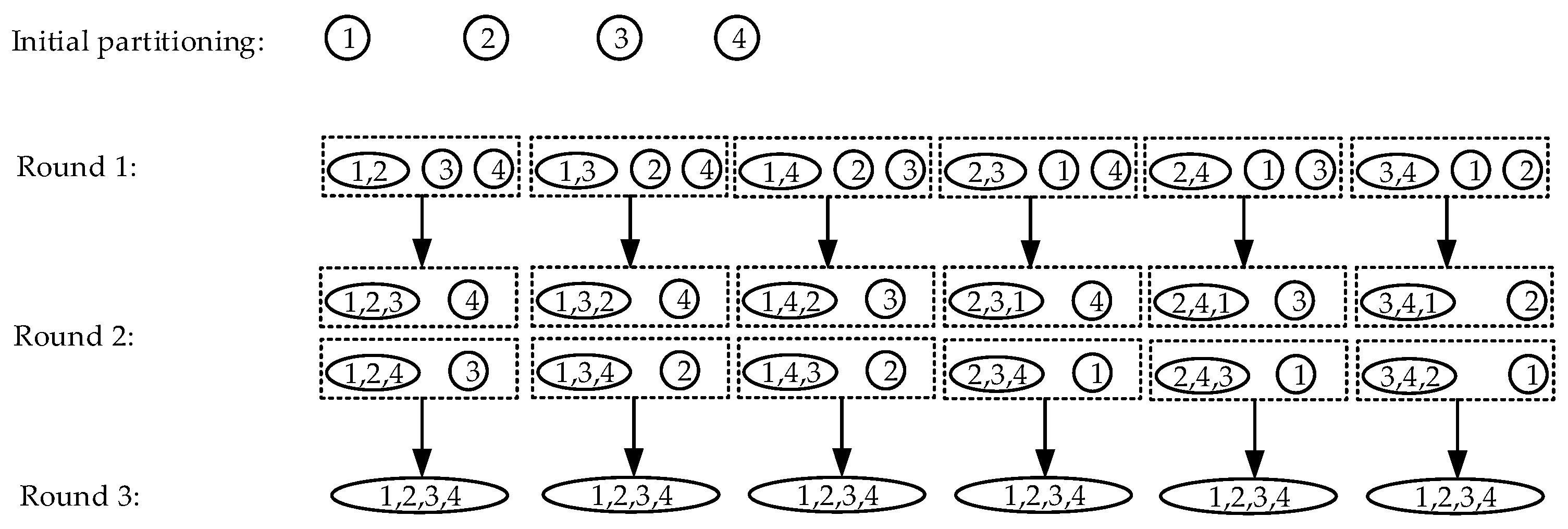
In the first round of partitioning, any two subpartitions, i and j, are randomly selected for merging to form candidate subpartition (i, j). The reactive-voltage modularity function is then computed for this candidate subpartition. Subsequently, the change in the modularity function for reactive-voltage partitioning is calculated for each (i, j) combination (six combinations in total). The subpartition (i*, j*) that yields the maximum positive value for is selected as the merger candidate for this iteration. The corresponding buses are formally assigned to the same subpartition and the reactive-voltage modularity function is updated accordingly.
For instance, if the candidate subdivision (1, 2) constitutes a partition satisfying , then (1, 2) shall be formally assigned to the same subdivision. In the second round of partitioning, for the three subpartitions (1, 2), 3, and 4, there are two possible combinations. If both combinations yield negative values for , this indicates that the first round of partitioning resulted in the optimal partition. Otherwise, the combination yielding the maximum positive value for is selected as the result of the second round of partitioning. For example, in the second round of partitioning, if the candidate subpartition (1, 2, 4) satisfies condition , then (1, 2, 4) is formally assigned to the same subpartition.
By the same token, in the third round of partitioning, the only remaining possible combinations are (1, 2, 3, 4). If is negative, then the optimal partition is the second-round result (1, 2, 4) and 3; otherwise, the optimal partition is (1, 2, 3, 4).
From the partitioning diagram of the four-bus system above, it can be observed that although the combination sequence between buses is randomised at each round, the algorithm traverses all possible combinations. Consequently, the partitioning outcome that maximises modularity is uniquely determined. Therefore, the optimal partitioning scheme obtained by the proposed adaptive reactive-voltage modularity partitioning model remains unaffected by the randomness that is inherent in the merging process.
Appendix A.2. Computational Process for Classical Holomorphic Embedding Power Flow
Appendix A.2.1. Fundamental Principles of Holomorphic Embedding
If the complex-variable function z(α) = u + jv, where α = x + jy, is differentiable everywhere within the domain D, and satisfies the Cauchy–Riemann Equation (A6), then z(α) is called holomorphic on D [36].
According to the concept of holomorphic embedding, the complex-variable function z(α) can be analytically expanded within its domain of convergence, as follows in the form of a Maclaurin series:
In the problem of solving the nonlinear equation f(z) = 0, substituting Equation (A7) enables the analytical reconstruction of the original equation:
Appendix A.2.2. Classical Holomorphic Embedding Power Flow Computational Model
The core concept of the holomorphic embedding approach to solving power flow lies in constructing nonlinear equations expanded in the complex domain as in Equation (A8). The classical holomorphic embedding power flow computational model is as follows:
where Si is the complex power at PQ bus; Pi represents the active power at PV bus; is the voltage setpoint amplitude at PV bus; is the voltage setpoint at the balancing bus, where slack denotes the balancing bus; Yij is the element in row i and column j of the bus admittance matrix; Vi denotes the voltage at bus i; α is the embedding factor characterising the load level; and ‘*’ denotes the conjugate operator.
Expanding the classical holomorphic embedding power flow model shown in Equation (A9) into a Maclaurin series, equating the coefficients of terms of the same order in the power series on both sides of the equation, and decomposing it into real and imaginary parts, ultimately transforms the power flow equation into a recursively solvable system of linear algebraic equations [37]:
where H is the highly sparse, stationary recursive relation matrix, which depends solely on network parameters and initial state values for recursion, thus requiring no updates during the recursive computation process; x[n] represents the nth-order power series coefficient vector to be determined; and b[n − 1] is the power series coefficient vector of an order no greater than n − 1, which is obtainable from the preceding recursive computation.
The specific expression for the recursive relationship matrix and the method for obtaining the initial values for the recursion are supplemented as follows:
where the superscripts PQ, PV, and slack are the sets of buses PQ, PV, and slack, respectively; [0] is the recursive initial value; the subscripts “re”and “im” denote the real and imaginary parts, respectively; and the meanings of the remaining variables are consistent with those in the main text.
The initial value calculation for classical holomorphic embedding is determined by setting zero injection at the PQ bus, ensuring that the PV bus operates without load and without active power generation, and adjusting reactive power injection at the PV bus to maintain constant voltage magnitude. This initial value may also be obtained by constructing the corresponding holomorphic embedding equations or using MATLAB’s MATPOWER toolbox.
Having obtained the initial value for the holomorphic embedding recurrence, the coefficients of the power series for each order of the state variable under investigation may be determined sequentially via the recurrence relation established by Equation (A12). This enables the explicit representation of the state variable as a power series, ultimately yielding its analytical expression:
where x is the vector of quantities to be determined, namely bus voltages and their reciprocals, reactive power at PV buses, and voltage stability indices, and M represents the order of iteration until convergence threshold is reached.
Upon obtaining the power series expression for the desired state variables, the power flow state variables at the base load level may be determined by directly substituting the target value α = 1 into Equation (A12). Subsequently, the obtained bus voltages are substituted into the power flow equations for verification. If the active power deviation at all buses falls below the threshold specified in Equation (A13), convergence is deemed to have been achieved and the recursion terminates. Otherwise, the solution proceeds to determine the coefficients of the next-order power series until the convergence criteria are satisfied.
where ΔPi is the active power deviation at bus I, and represents the convergence threshold, which is set to 10−6 in this paper.
Appendix A.3. The Selection Process of the Pareto Solution Set
First, the range of each objective value in the Pareto solution is normalised to eliminate the influence of units:
where fij is the j-th objective value for the i-th solution, and ε = 10−10 is employed to prevent zero-division errors.
Secondly, we calculate the information entropy of each objective and thereby derive its objective weight in the decision-making process:
where N is the number of solutions.
Subsequently, a weighted decision matrix is constructed using entropy weights. Each column of the normalised decision matrix Y is multiplied by its objective weight Wj = 1 − Ej, calculated from its information entropy E, thereby yielding the weighted matrix V, where Vij = WjYij.
Then, we calculate the Euclidean distances Sf and Sz from each solution to the ideal optimum and worst points, respectively, and construct a composite indicator:
where Ci simultaneously reflects the degree of proximity to the ideal point and distance from the worst point.
Finally, the solution with the smallest Ci is selected as the final configuration scheme, as it achieves the optimal trade-off among multiple objectives.
Appendix B
Appendix B.1. UPQC Optimal Configuration for a Real-World Distribution Networks
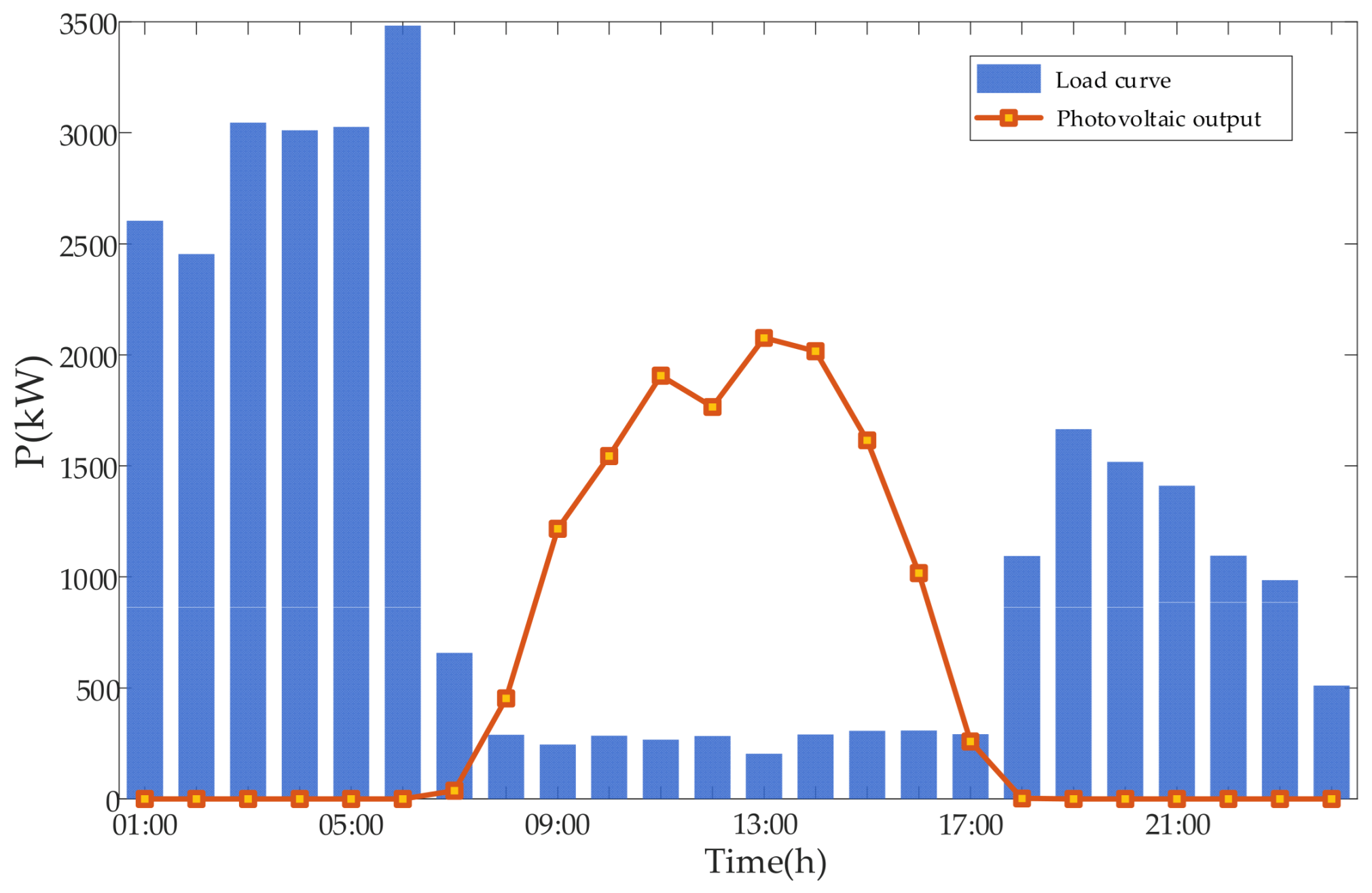
The 10 kV Tuji feeder located in Longyan City, Fujian Province, China, is selected as the study object. The effectiveness of the proposed UPQC optimal configuration method in mitigating voltage limit violations is evaluated based on this feeder. On 14 May 2024, which is considered a representative day, the region experienced favourable solar irradiance conditions. The total exported energy of the feeder reached 25,080.3 kW·h. As a result, the voltage compliance rate of low-voltage users was only 85.14%. As shown in Figure A2, the aggregated output of distributed photovoltaics exceeds the local load demand during most periods. Consequently, the feeder exhibits pronounced reverse power flow behaviour. The corresponding typical-day DG and load data for the Tuji feeder are provided in Table 2.
Figure A2.
Typical daily scenario for the Tuji feeder.
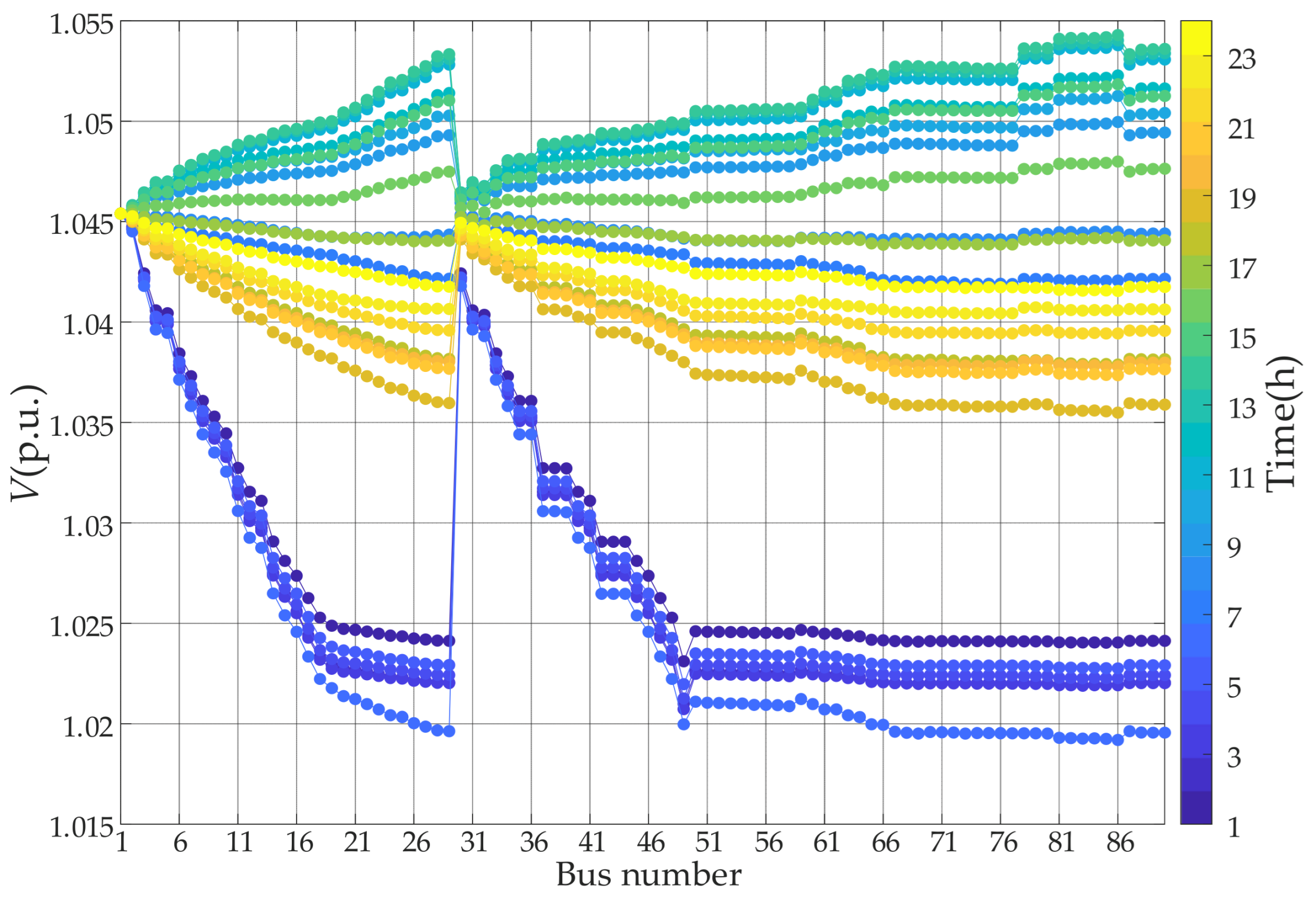
As illustrated in Figure A3, after the integration of distributed photovoltaics into the Tuji feeder, voltage levels exceed the upper limit of 1.05 p.u. during certain periods. This operating condition is unfavourable for the safe and stable operation of the distribution network. Therefore, it is necessary to mitigate the voltage violations through a rational configuration of UPQC.
Figure A3.
Voltage curve for a typical daily scenario at the Tuji feeder.
The topology of the Tuji feeder is shown in Figure A4. Based on the reactive power–voltage sensitivity partitioning results listed in Table A1, the feeder is divided into Zone 2 and Zone 1 in descending order of the sensitivity metric.
Figure A4.
Topology of the Tuji feeder.
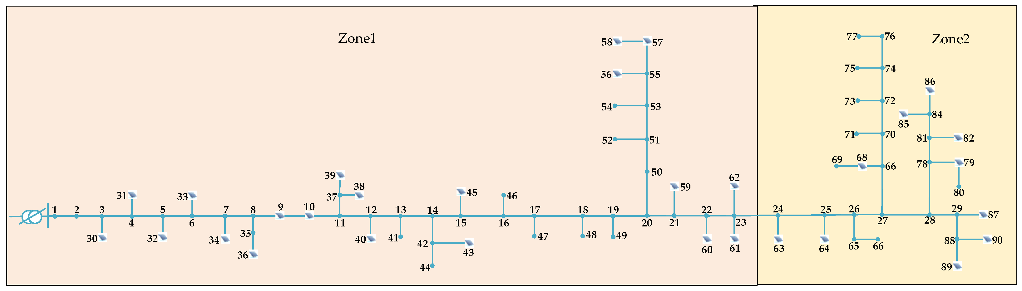
Table A1.
Partition sensitivity index of the Tuji feeder.
Subsequently, weak-bus identification is performed for the representative daily scenarios of the Tuji feeder. The corresponding results are presented in Table A2.
Table A2.
Results of weak bus identification in Tuji feeder.
The number of installed UPQC units was set to one to clearly demonstrate the intrinsic voltage regulation capability of a single device and to reflect the conservative deployment strategy that is typically adopted in practical distribution network planning. The allowable capacity range of the shunt compensation module of a single UPQC is specified as 0–1.0 MVar. The installation cost of UPQC is set as 1.3 CNY/Var for capacities below 200 kVar, 0.9 CNY/Var for capacities between 200 and 400 kVar, 0.55 CNY/Var for capacities between 400 and 500 kVar, and 0.4 CNY/Var for capacities exceeding 500 kVar. The discount rate is set to 0.05. The annual maintenance cost is assumed to be CNY 750 per unit. All remaining parameters are consistent with those of the extended IEEE-33 bus power system.
Zone 2, which exhibits the highest reactive power–voltage sensitivity, is selected as the candidate area for UPQC installation. The bi-level optimisation model is then solved to determine the installation location and capacity of the UPQC. The representative daily voltage profiles of the Tuji feeder after optimisation are illustrated in Figure A5. The corresponding optimal configuration results are summarised in Table A3.
Figure A5.
Optimised voltage curve for the Tuji feeder.
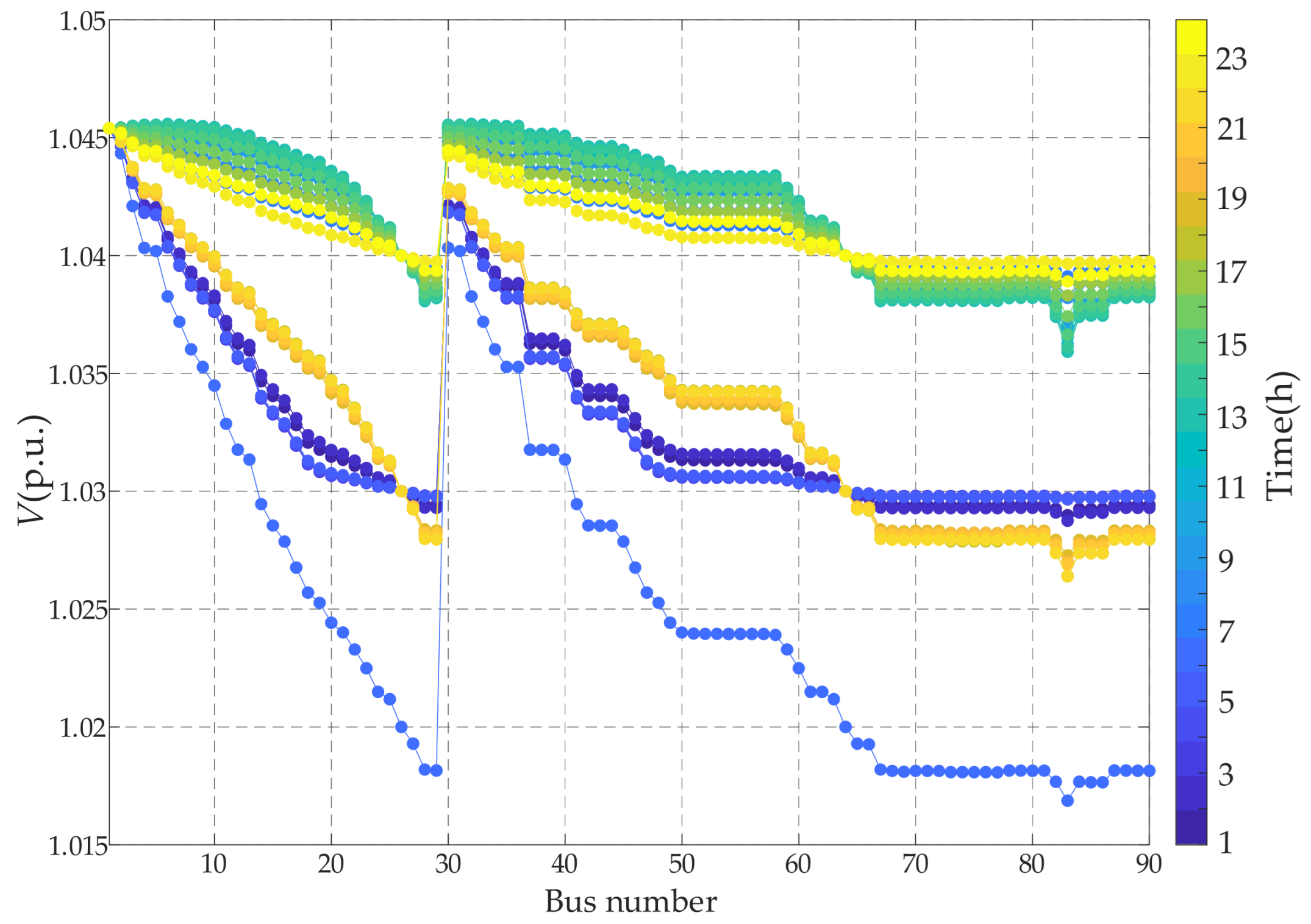
Table A3.
Optimised configuration results.
The simulation results indicate that installing a 100 kVar UPQC at Bus 26 of the Tuji feeder effectively mitigates the voltage limit violations caused by the integration of distributed photovoltaics. After optimisation, the voltages at all buses remain within the limit of 1.05 p.u. Moreover, the overall voltage deviation is reduced from 7.4176 p.u. to 6.9118 p.u., corresponding to a reduction of 6.82%. These results demonstrate a noticeable improvement in voltage quality across the system.
These results suggest that the proposed UPQC optimal configuration method is applicable to practical distribution feeders with high photovoltaic penetration. The method demonstrates the potential to mitigate voltage violations under real-world operating conditions, while requiring only a relatively small UPQC capacity.
Appendix B.2. Comparison of Computational Efficiency with and Without Network Partitioning
To compare the optimisation efficiency with and without network partitioning, the extended IEEE-33 bus power system used Zone 5, while the real-world distribution network used Zone 2 as candidate locations for a single UPQC, with both zones identified as the most sensitive. In contrast, without partitioning, all buses in the network were considered as potential candidate locations for the UPQC. Key buses for evaluating voltage regulation in the lower level model were selected based on the weak-bus identification results in Table 2 and Table A2. Simulation results showed that, even without partitioning, the UPQC was ultimately deployed in the region with the highest reactive power–voltage sensitivity, and the optimisation outcomes were identical in both cases. The computational time for solving the bi-level UPQC optimal configuration model was recorded using MATLAB’s tic–toc function. Table A4 presents the total computational time for the two scenarios.
Table A4.
Total runtime comparison.
The adoption of network partitioning reduced the solution search space, thereby improving optimisation efficiency by 24.8% in the extended IEEE-33 bus system and by 29.7% in the practical distribution network, compared with that without partitioning.
Appendix C
Table A5.
Data of DG–load power for the extended IEEE-33 bus power system on a typical day.
Table A6.
Data of DG–load power for the Tuji feeder on a typical day.
References
- Liu, J.; Sun, K.; Ding, Z.; Li, K.; Sun, Y. Multi-stage planning of distribution network with high penetration renewable energy considering reliability index. IEEE Trans. Ind. Appl. 2023, 60, 2344–2356. [Google Scholar] [CrossRef] [Scilit]
- Wu, R.; Liu, S. Robust Optimisation of Active Distribution Networks Considering Source-Side Uncertainty and Load-Side Demand Response. Energies 2025, 18, 3531. [Google Scholar]
- Ma, M.; Huang, H.; Song, X.; Peña-Mora, F.; Zhang, Z.; Chen, J. Optimal sizing and operations of shared energy storage systems in distribution networks: A bi-level programming approach. Appl. Energy 2022, 307, 118170. [Google Scholar] [CrossRef] [Scilit]
- Wang, Z.; Ge, L.; Ding, J.; Gu, W. Distributed Newton-based voltage control method for high-penetration PV generation cluster in active distribution networks. IET Renew. Power Gener. 2020, 14, 1904–1911. [Google Scholar] [CrossRef] [Scilit]
- Gao, X.; Zhang, J.; Sun, H.; Liang, Y.; Wei, L.; Yan, C.; Xie, Y. A Review of Voltage Control Studies on Low Voltage Distribution Networks Containing High Penetration Distributed Photovoltaics. Energies 2024, 17, 3058. [Google Scholar] [CrossRef] [Scilit]
- Tang, F.; Xie, J.; Liu, C.; Lin, Z.; Qi, J.; Liu, Z.; Deng, H. PV hosting capacity evaluation of distribution networks based on holomorphic embedding method. Power Syst. Technol. 2024, 48, 291–303. [Google Scholar]
- Feng, N.; Niu, T.; Yan, J.; Zhang, Y.; Feng, Y.; Lei, Y. Optimal Placement and Sizing of Reactive Power Compensation Devices in Power Grids with High Penetration of Distributed Generation. Processes 2025, 13, 2953. [Google Scholar] [CrossRef] [Scilit]
- Mao, X.; Zhu, W.; Wu, L.; Zhou, B. Optimal allocation of dynamic VAR sources using zoning-based distributed optimisation algorithm. Int. J. Electr. Power Energy Syst. 2019, 113, 952–962. [Google Scholar] [CrossRef] [Scilit]
- Gan, D.; Ling, H.; Mao, Z.; Gu, R.; Zhou, K.; Lin, K. A Network Partition-Based Optimal Reactive Power Allocation and Sizing Method in Active Distribution Network. Processes 2025, 13, 2524. [Google Scholar] [CrossRef] [Scilit]
- Xu, Z.; Tang, Z.; Chen, Y.; Liu, Y.; Gao, H.; Xu, X. Optimal robust allocation of distributed modular energy storage system in distribution networks for voltage regulation. Appl. Energy 2025, 388, 125625. [Google Scholar] [CrossRef] [Scilit]
- Gallego, L.; López-Lezama, J.; Gómez Carmona, O. A mixed-integer linear programming model for simultaneous optimal reconfiguration and optimal placement of capacitor banks in distribution networks. IEEE Access 2022, 10, 52655–52673. [Google Scholar] [CrossRef] [Scilit]
- Ganguly, S. Multi-Objective Planning for Reactive Power Compensation of Radial Distribution Networks with Unified Power Quality Conditioner Allocation Using Particle Swarm Optimisation. IEEE Trans. Power Syst. Publ. Power Eng. Soc. 2014, 29, 1801–1810. [Google Scholar] [CrossRef] [Scilit]
- Guo, Q.; Wu, J.; Mo, C.; Xu, H. A model for multi-objective coordination optimisation of voltage and reactive power in distribution networks based on mixed integer second-order cone programming. Proc. CSEE 2018, 38, 1385–1396. [Google Scholar]
- Guo, H.; Che, Y. Active Distribution Network Bi-Level Programming Model Based on Hybrid Whale Optimisation Algorithm. Sustainability 2025, 17, 8560. [Google Scholar] [CrossRef] [Scilit]
- Zhang, H.; Lin, S.; Liu, M. Robust Optimal Allocation of Reactive Power Compensation in Low Voltage Distribution Networks Considering Uncertainty of Photovoltaic Generation. Power Syst. Technol. 2016, 40, 3880–3888. [Google Scholar]
- Chen, X.; Zhang, X.; Yan, Q.; Li, Y. Spatio-Temporal Adaptive Voltage Coordination Control Strategy for Distribution Networks with High Photovoltaic Penetration. Energies 2025, 18, 2093. [Google Scholar] [CrossRef] [Scilit]
- Lin, S.; Wu, J.; Mo, C.; Wang, Z.; Guo, Q. Dynamic partition and optimisation method for reactive power of distribution networks with distributed generation based on second-order cone programming. Power Syst. Technol. 2018, 42, 238–246. [Google Scholar]
- Li, X.; Gao, J. Improved particle swarm optimisation algorithm for multi-objective reactive power optimisation of distribution network. Electr. Power Autom. Equip. 2019, 39, 106–111. [Google Scholar]
- Meng, L.; Yang, X.; Zhu, J.; Wang, X.; Meng, X. Network partition and distributed voltage coordination control strategy of active distribution network system considering photovoltaic uncertainty. Appl. Energy 2024, 362, 122846. [Google Scholar] [CrossRef] [Scilit]
- Zhou, X.; Wang, S.; Zhang, W.; Wang, J.; Qin, R.; Li, S. Multi-objective optimisation of fixed series compensation in distribution network. Power Syst. Prot. Control. 2017, 45, 115–122. [Google Scholar]
- Liu, Q.; Huang, J.; Wang, S. Compounding voltage weakness indicator and reactive power optimisation strategy oriented to it. Electr. Power Autom. Equip. 2024, 44, 147–152+159. [Google Scholar]
- Alhejji, A.; Ebeed, M.; Kamel, S.; Alyami, S. Optimal Power Flow Solution with An Embedded Center-node Unified Power Flow Controller Using An Adaptive Grasshopper Optimisation Algorithm. IEEE Access 2020, 8, 119020–119037. [Google Scholar] [CrossRef] [Scilit]
- Zhu, X.; Guo, Y.; Li, A.; Li, S.; Zhang, J.; Gu, B.; Deng, J. Two-stage robust optimisation of unified power quality conditioner (UPQC) siting and sizing in active distribution networks considering uncertainty of loads and renewable generators. Renew. Energy 2024, 224, 120197. [Google Scholar] [CrossRef] [Scilit]
- Wang, Y.; Zhong, Q.; Liu, Y.; Tu, C.; Zhang, H. Review and Prospects of Key Technologies for Power Quality Disturbance Mitigation in New Power System. Proc. CSEE 2025, 45, 8670–8691. [Google Scholar]
- Ray, P.; Ray, P.; Dash, S. Power quality enhancement and power flow analysis of a PV integrated UPQC system in a distribution network. IEEE Trans. Ind. Appl. 2021, 58, 201–211. [Google Scholar] [CrossRef] [Scilit]
- Xiao, C.; Zhao, B.; Zhou, J.; Li, P.; Ding, M. Network partition based cluster voltage control of high-penetration distributed photovoltaic systems in distribution networks. Autom. Electr. Power Syst. 2017, 41, 147–155. [Google Scholar]
- Liu, C.; Lai, Q.; Yao, L.; Xu, J.; Sun, Y. Power system decoupling model based on holomorphic embedding method: Weak bus identification. Proc. CSEE 2022, 42, 1736–1748. [Google Scholar]
- Liu, C.; Luo, Y.; Dong, X. Voltage stability margin evaluation algorithm based on holomorphic embedded and padé approximation zero-pole detection. Power Syst. Technol. 2024, 48, 3790–3800. [Google Scholar]
- He, S.; Shao, Z.; Zheng, W.; Chen, F.; Li, Y. Bi-level uncertain reactive power planning of distribution network considering SVG dynamic voltage regulation strategy. Power Syst. Technol. 2023, 47, 5158–5170. [Google Scholar]
- Gao, H.; Liu, J.; Shen, X.; Xu, R. Optimal power flow research in active distribution network and its application examples. Proc. CSEE 2017, 37, 1634–1645. [Google Scholar]
- Zhang, Z.; Nian, H.; Li, P.; Ma, Z. Voltage compensation capability analysis and improvement method for unified power quality conditioner with energy storage. Autom. Electr. Power Syst. 2022, 46, 151–159. [Google Scholar]
- Khadkikar, V. Enhancing Electric Power Quality Using UPQC: A Comprehensive Overview. IEEE Trans. Power Electron. 2012, 27, 2284–2297. [Google Scholar] [CrossRef] [Scilit]
- Haddadian, H.; Noroozian, R. Multi-microgrids approach for design and operation of future distribution networks based on novel technical indices. Appl. Energy 2017, 185, 650–663. [Google Scholar] [CrossRef] [Scilit]
- Yang, D.; Pan, G.; Zhang, J.; He, J.; Zhang, Y.; Xiao, C. Double-Layer Optimal Configuration of Wind–Solar-Storage for Multi-Microgrid with Electricity–Hydrogen Coupling. Processes 2025, 13, 3263. [Google Scholar] [CrossRef] [Scilit]
- Cai, M.; Zeng, T.; Zeng, L.; Zhou, X.; Huang, X. Optimised Two-Layer Configuration of SESS-CCHP System Considering Wind and Light Output Correlation and Load Sensitivity. Energies 2024, 17, 4638. [Google Scholar] [CrossRef] [Scilit]
- Shao, Z.; Li, Y.; Yan, X.; He, S.; Chen, F. Affine power flow algorithm for power system based on holomorphic embedding method. Proc. CSEE 2024, 44, 105–117. [Google Scholar]
- Rao, D.; Tylavsky, J.; Feng, Y. Estimating the saddle-node bifurcation point of static power systems using the holomorphic embedding method. Int. J. Electr. Power Energy Syst. 2017, 84, 1–12. [Google Scholar] [CrossRef] [Scilit]

Disclaimer/Publisher’s Note: The statements, opinions and data contained in all publications are solely those of the individual author(s) and contributor(s) and not of MDPI and/or the editor(s). MDPI and/or the editor(s) disclaim responsibility for any injury to people or property resulting from any ideas, methods, instructions or products referred to in the content. |
© 2026 by the authors. Licensee MDPI, Basel, Switzerland. This article is an open access article distributed under the terms and conditions of the Creative Commons Attribution (CC BY) license.