


Abstract
Previous studies have applied particle swarm optimization to coupled offshore wind farm layout and cable design and used geometry-guided genetic search to preserve spatial configurations during crossover. Transferring a successful relocation between layouts requires reassessing its wake and cable effects in the receiving layout. We propose cross-swarm recombination particle swarm optimization (CSRPSO) for offshore layouts with embedded capacity-constrained routing under a levelized cost of energy (LCOE) objective. Two swarms use wake interactions and cable connections to guide turbine relocations. Successful relocations are reconstructed in the other swarm’s personal-best layouts and compared with candidates generated from current layouts using complete LCOE evaluations. Six algorithms were compared across eight wind-farm cases over 30 repetitions per case, using matched seeds and initial populations, populations of 30 and 15,000 complete evaluations including initialization. CSRPSO achieved the lowest mean and median LCOE in every case, reducing mean LCOE by 0.041–0.697% versus adaptive replacement strategy-incorporated genetic learning particle swarm optimization (AGPSO), the closest baseline. At 10,000 evaluations, one-third below budget, its mean LCOE was below AGPSO’s final mean in every case. Mean annual energy production exceeded AGPSO’s in all eight cases, and mean cable expenditure was lower in six.
1. Introduction
Wind speed and direction influence turbine energy output through their effects on the incident flow and wake exposure [1]. For a given layout, the turbine power curve converts the resulting effective wind speed into power output. The joint occurrence frequencies of wind speed and direction weight these outputs in the annual energy calculation (Section 2.2) [2].
The International Energy Agency estimated a global offshore wind technical generation potential exceeding 420,000 TWh per year. That 2019 assessment highlighted high-quality offshore wind resources and reported capacity factors of 40–50% for new offshore projects, exceeding those of onshore wind [3]. Gigawatt-scale offshore wind developments also affect power-system adequacy, which concerns the availability of sufficient generation capacity to meet demand at a specified reliability level. Capacity credit quantifies their contribution to adequacy and can be expressed as a share of installed capacity; its assessment uses time-aligned hourly generation and demand data [4]. The IEA’s 2019 assessment found that the high capacity factors and seasonality of offshore wind allow 30% or more of its capacity to be counted towards reliability requirements, a higher share than for onshore wind and solar PV, reducing the need for other dispatchable capacity [3]. The present study does not evaluate capacity credit or system adequacy; it addresses the farm-level layout and cable design that determine how much energy a given installed capacity delivers and at what cost.
The economic use of offshore wind depends on balancing lifetime energy production against turbine, foundation, electrical, installation, and operating costs [5]. Climate-related changes in wind conditions also influence lifetime energy estimates for turbines operating over several decades. Nicolosi and Tina evaluated a single turbine at three offshore locations south of Sicily and projected reduced annual production at two locations [6]. Layout and cable design contribute to this balance: spreading turbines can reduce wake losses while increasing collection-system expenditure [7,8].
Aerodynamic and electrical interactions respond differently to a relocation. Site geometry, spacing, and wind conditions constrain energy capture, while capacity-constrained collection networks determine connection costs [9]. Topology and substation location shape routing [10]; wind-dependent losses can affect cable cross-section selection [11]; and downstream turbine counts determine required capacity [12]. With turbine and substation locations fixed, binary integer programming has jointly selected collection-network topology and cable types under a life-cycle cost objective [13]. Consequently, even with fixed turbine count and substation location, moving one turbine can change wake exposure, feeder membership, and cable type.
Joint-design methods connect these decisions in several ways. Reviews have summarized offshore layout and electrical-system design methods [14], and the TOPFARM framework optimizes layouts for lifetime profit using multi-fidelity models of energy production, wake-induced fatigue, and electrical-grid and foundation costs [15]. Bilevel multiobjective optimization assigns cabling to a subordinate problem [16], while hybrid evolutionary search uses mixed-integer programming to optimize the network for each candidate layout [17]. Integrated formulations include mixed-integer linear programming with branch-and-cut [18], a mixed-integer quadratically constrained model with bilevel decomposition [19], and a quota Steiner tree model incorporating wake interference [20]. These approaches assess complete designs. Sharing a partial relocation between designs introduces a further problem: its source-layout benefit need not persist after the surrounding turbines and network change.
Particle swarm optimization (PSO) has been applied to turbine placement in large-scale offshore wind farms [1] and to offshore layouts whose electrical infrastructure, annual energy production, and cost are evaluated under a levelized cost of energy (LCOE) criterion [2]. Zhang et al. used enhanced PSO in a bilevel framework for non-uniform offshore turbine layouts and cable routing under a refined LCOE objective [21]. Qi et al. combined Voronoi-based connection candidates, adaptive PSO, and local search to minimize cable capital and power-loss costs for heterogeneous offshore wind farms with fixed turbine positions [22]. Lei et al. combined genetic learning with adaptive replacement of the worst-performing turbine to improve wind-farm energy conversion efficiency [23]. For coupled layout and cable design, spatially informed search offers useful relocation operators. Joint turbine and cable moves expose their economic consequences during search [7]. Geometry-guided genetic search preserves spatial configurations through sector-based crossover and uses capacity-constrained routing [24]. Geometry-guided multiobjective search combines variation with balance-aware selection between energy production and capital expenditure [25]. For a fixed turbine count, transferring selected sites additionally requires receiver-specific removals and spacing checks.
Other wind-farm optimizers share information through different representations. Turbine-level differential evolution represents a complete layout by its population [26]; discrete differential evolution exchanges information between fitness-stratified populations [27]; reinforcement-learning-based PSO adapts parameters from an experience pool [28]; and incremental surrogate-assisted differential evolution updates a Kriging model of complete-layout LCOE [29]. A multi-team comparison of eight gradient-based, gradient-free, and hybrid methods on a common layout problem found similar performance when each method was applied by experienced users with the same objective function [30]. In the occupancy representation considered here, the shared object is a feasible exchange of selected sites. Its application depends on which donor targets the receiver already occupies and which existing sites can be removed.
PSO links movement to personal and social learning [31]. Comprehensive learning selects dimension-specific personal-best exemplars [32], and heterogeneous comprehensive learning separates exemplar sources for exploration and exploitation [33]. Dimension-group elite learning coordinates random variable groups [34], whereas variable interaction graphs infer dependencies from particle movements [35]. In layout and cable design, wind-dependent wake relationships and the decoded collection network supply two physical groupings. They define complementary exchange neighborhoods while retaining a common complete-layout objective.
The receiving context determines the value of an inherited exchange. Cooperative PSO evaluates components within a complete context vector assembled from subpopulation solutions [36]. Here, each particle already represents a complete layout. Its frozen personal best provides the context for reconstructing successful donor targets, while its current position generates a native candidate. Preserving targets already present, adapting removals to the receiver, and comparing the two fully evaluated candidates make reuse conditional on the receiver’s balance between cost and energy. Section 3.3 details this comparison.
This construction also determines what PSO should remember. Physical grouping, feasibility checks, and candidate competition can alter the intended move. Memory based on the selected occupancy displacement therefore carries the executed trajectory into subsequent learning, while separate best-so-far archives retain evaluated improvements, as described in Section 3.4.
Here, we develop cross-swarm recombination particle swarm optimization (CSRPSO), a PSO variant for offshore layout design with embedded capacity-constrained routing. The design retains PSO’s personal-best and social learning [31], while replacing direct continuous position updates with feasible site exchanges that preserve turbine count and spacing. We use cross-swarm recombination to reuse successful exchanges while reassessing their wake and cable effects in the receiving layout. Successful exchanges from the other swarm are reconstructed in the receiving particle’s frozen personal-best layout and compared with current-position native search using complete LCOE evaluation. Motion memory then records the selected occupancy displacement. The contributions are:
- (i)
- Receiver-specific cross-swarm recombination. A successful native exchange supplies targets and associated donor removals. Targets are reconstructed in the receiver’s frozen personal best, retaining those already occupied and matching missing targets to receiver-specific removals. The reconstruction competes with current-position native search after complete economic evaluation.
- (ii)
- Physical exchange construction. Wake and feeder neighborhoods organize the native exchanges shared between swarms. Matched removals and insertions preserve turbine count, and spacing checks preserve admissibility. A uniform single-exchange fallback supplies a nonzero native proposal whenever an admissible pair exists.
- (iii)
- Executed-displacement memory. The selected occupancy change updates motion memory; both evaluated candidates update best-so-far archives. For zero initial memory and inertia in , memory has a componentwise unit bound and occupancy-consistent signs, while archive values are nonincreasing.
The remainder of this paper is organized as follows. Section 2 formulates the coupled layout and cable design problem. Section 3 details CSRPSO. Section 4, Section 5 and Section 6 present the experimental protocol, results, and discussion and conclusions, respectively. The appendices establish the analytical properties of CSRPSO (Appendix A) and compare performance at smaller evaluation budgets (Appendix B).
2. Problem Formulation
2.1. Site Inputs and Feasible Layouts
Let denote the prescribed site domain after exclusion zones have been removed. Let be candidate turbine coordinates in metres, M the prescribed turbine count, a fixed offshore substation, and the required spacing. Candidate occupancy is represented by , with selected set .
Define
The wind input is a discrete joint distribution over directions and free-stream speeds , satisfying and . The case-specific candidate domains and wind distributions are specified in Section 4.1.
2.2. Wake and Energy Evaluation
Jensen’s report provides a foundational engineering model of expanding turbine wakes [37]. The reference evaluator uses centre-point wake coverage and multiplicative velocity factors. For direction , rotate each coordinate by . For source turbine i and receiving turbine j, define downstream separation and cross-stream separation . Angles are supplied in radians. For rotor radius R, thrust coefficient , and wake expansion coefficient k, define
The implemented reference values are and . Effective speed and annual energy production (AEP) are evaluated as
Here P is the supplied power curve, evaluated by cubic-spline interpolation within the interval bounded by its cut-in and cut-out speeds and set to zero outside that interval. Power in kilowatts gives AEP in kilowatt-hours per year. Equation (2) also defines the wake swarm’s directed adjacency, so neighborhoods are constructed without a separate aerodynamic surrogate.
2.3. Embedded Capacity-Constrained Routing
The deterministic routing map sorts selected turbines counterclockwise about from the positive x-axis over . Angle ties are broken by squared distance to , then x and y, in ascending order. From the first turbine, consecutive groups contain turbines, except possibly the last. Each group’s Euclidean minimum spanning tree connects to the substation through its nearest turbine. Removing the substation identifies the feeder groups used for learning. This project-specific decoder is a Sweep-based construction of the type studied by Cazzaro et al. [12].
Orient the network away from the substation. For each edge e, let be the number of downstream turbines and its length. Given strictly increasing cable capacities , expressed in turbine counts, and the corresponding prices per metre , the decoder assigns
Turbine occupancies are the search variables. Both swarms use the same decoder for objective evaluation; the collection swarm additionally derives its exchange neighborhoods from the current decoded network. Every full evaluation reconstructs the network.
The Sweep construction, which originated in vehicle routing, where customers are grouped by polar angle before each group is routed [38], was chosen for three reasons. First, the layout search requires a routing step in every complete evaluation, and the 1440 runs reported here performed 21.6 million such evaluations. For each baseline, the total wall time of its 240 runs was less than 2 ms per complete evaluation, a figure that also includes the search operations (Section 5.5); a mixed-integer routing model would instead require a solver call in every evaluation. Second, the decoder is deterministic, so repeated evaluations of a layout return the same objective value, as assumed by the archive analysis in Appendix A. Third, it always returns a capacity-feasible radial network whose feeders define the collection swarm’s neighborhoods. The decoded network is therefore a consistent cost model for comparing layouts rather than an optimal cable design. Optimization-based routing methods [13,18] can find lower-cost networks for a given layout and can be applied to the selected layouts after the search; another tree-structured router could also replace the decoder within CSRPSO, with its feeders defining the collection neighborhoods.
2.4. Integrated Economic Objective
Let Y be project lifetime and r the discount rate. With a stationary annual wind distribution, discounted energy is
In the reference cost calculation, all turbine specifications, sea depth, export-cable length, and substation inputs are fixed within each case. The layout-dependent cost can then be written as
Here includes turbine, foundation, installation, substation, project-management, decommissioning, and discounted operation and maintenance costs, together with their fixed additional-cost terms, in euros. The evaluator uses , , and ; the last value accounts for the cable-linked additional-cost term. Case-specific values of are specified in Section 4.1. CSRPSO requires finite positive objective values and uses the same F for both swarms.
Equation (6) follows the discounted cash-flow definition of LCOE as the ratio of discounted lifetime costs to discounted lifetime energy [39,40]. Investment costs are incurred at the start of operation, annual operation and maintenance costs are discounted over the project lifetime, and the annual energy yield is constant. Detailed techno-economic tools additionally resolve replacement costs, degradation, component lifetimes, and time-varying production. These items are not modelled here because the compared layouts share the same turbines, substation, and lifetime. Layout-independent cash flows, such as turbine replacements or financing costs, change only , whereas a degradation or availability factor applied equally to all layouts scales and leaves percentage differences in F unchanged. Section 5.1 re-evaluates the final layouts under alternative cost assumptions.
3. Cross-Swarm Recombination Particle Swarm Optimization
CSRPSO builds on personal-best and social learning in PSO [31] and on cooperation between swarms [36]. The contribution developed here is receiver-specific recombination of successful turbine exchanges between two swarms that each maintain complete layouts. Wake and feeder relationships define the native exchanges, while the receiver’s frozen personal best supplies the reconstruction context. Eligible reconstructions compete with native candidates generated from current layouts through complete LCOE evaluation under Equation (6); motion memory records the selected occupancy displacement.
3.1. Particle State and Learning Intent
CSRPSO maintains an even number of particles in two fixed, equally sized swarms: the wake swarm and the collection swarm . Their exchanges use wake and feeder relationships, respectively. Each particle stores a feasible occupancy vector , motion memory , and personal best . Here t counts updates of particle i. The current position supports continued exploration, the personal best retains the particle’s best evaluated configuration, and the swarm best supplies social guidance within that swarm. A global archive determines the returned solution. After evaluating the shared feasible initial population, randomly partition the particles into the two swarms and initialize motion memory to zero. The default coefficients are and .
Set-based PSO establishes a precedent for redesigning positions and movement operators in discrete domains [41]. Xu et al. use differences between binary feature subsets to identify activation and deactivation positions in bee-colony search [42]. CSRPSO retains real-valued site preferences and converts them into fixed-count exchanges. Before updating a particle, freeze its personal best, its swarm best, and the other swarm’s available exchange record. This keeps the learning references, reconstruction context, and benchmark for recording successful exchanges fixed while the new candidates are evaluated. The learning intent is
where , , and the components of are sampled independently from . The intent layout is
The operator selects the M largest scores, so the intended insertions and removals have equal cardinality. Ties favor currently occupied positions and then ascending candidate indices, retaining existing occupancy when the scores give no preference for a change. The intent specifies preferred sites; the following exchange construction determines which changes can be executed together under the spacing constraints.
3.2. Native Exchanges and Feasible Single-Exchange Fallback
The intent identifies a destination set but does not assign destinations to the turbines being removed. Let and . Pair with through a bijection minimizing total squared distance. This geometric correspondence gives each removal one insertion, allowing physical groups to select complete relocations while retaining turbine count. Source indices are ordered increasingly; equal-cost matchings are resolved lexicographically by target indices. A native block is
Write for the occupancy vector of .
Two grouping rules connect these relocations to the physical model. For a wake particle, sample with probability . For each seed , group it with proposed removals satisfying or . This includes its direct upstream and downstream interactions among the proposed removals. The sampled direction determines the neighborhood; complete AEP evaluation still uses the full wind distribution in Equation (3). For a collection particle, group the seed with proposed removals in its current feeder, identified by removing the substation from the decoded network. Before relocation, these positions share a collection branch whose subsequent connections and loading are recomputed during full evaluation.
Enumerate the distinct seed-generated blocks, retain those whose complete layouts satisfy , and select uniformly among them. Deduplication prevents a block from receiving extra sampling weight merely because several seeds generate it. Reject an infeasible block as a whole, preserving the complete set of paired changes as the unit tested. If there is no feasible block, the provisional native candidate is S.
A repeated intent or rejected physical blocks can leave the layout unchanged even when a feasible single relocation exists. The fallback checks this remaining opportunity directly. Whenever native construction leaves the layout unchanged, form
where denotes the occupancy vector of a set H. If is nonempty, sample one pair uniformly and set ; otherwise retain . The fallback can use targets outside the original intent and requires no accumulated stagnation count. The native candidate undergoes one full evaluation in every update.
A nonzero native exchange is recorded as successful when , using the frozen personal-best value. The exchange must therefore advance the source particle’s best attained objective, rather than merely improve on a poorer current position. Each swarm stores its latest successful native exchange, including the correspondence between removals and insertions and the source coordinates. Successful exchanges can originate from either a physical block or the single-exchange fallback. Recording only native exchanges preserves the link between a shared operation and its directly evaluated source candidate; recombination outcomes update the solution archives described below.
3.3. Personal-Best Recombination and Candidate Competition
The key step introduced here is receiver-specific reconstruction of a successful exchange from the other swarm in the receiving particle’s frozen personal-best layout. Donor targets already present are retained, while receiver-specific removals are selected for the missing targets. A feasible reconstruction that introduces at least one previously missing donor target competes with the native candidate generated from the receiver’s current position after complete LCOE evaluation. This tests the transferred operation in the receiving layout, where its wake and cable effects are recomputed.
Let be the receiving particle’s frozen personal-best layout. Recombination uses the other swarm’s latest successful native exchange available at the start of this update. Let be the donor’s complete target set, and let identify the recorded donor removal paired with target a. Targets already in P remain satisfied. Define the missing targets and the removable set . Match the source coordinates associated with to distinct positions in H:
The assignment aligns relinquished donor sites with removable recipient sites, while H protects donor targets already present in P. Rows follow ascending missing-target indices, and equal-cost assignments use the lexicographically smallest removal-index sequence. The recombined layout is
Write for the occupancy vector of . Because , enough removable positions exist. This construction retains every donor target in . The complete recombined layout is checked for spacing feasibility and, if feasible and budget remains, receives full wake and routing evaluation.
Define when a donor record exists, , and the resulting feasible recombination has been evaluated within the budget; otherwise set . Candidate selection is
If , then : the donor has introduced no missing target. This unchanged personal best is still fully evaluated when budget permits, but excludes it from position competition. This qualification prevents a return to the unchanged personal best from displacing the native proposal solely because of its previously attained objective value. Nonzero recombination is defined relative to P; the selected layout can still coincide with the particle’s old current position.
Write , , , and , where the superscripts label the native and recombined candidates, respectively. Their economic comparison satisfies
For and , recombination wins exactly when . A gain in discounted energy can justify added lifetime cost below this threshold; an energy reduction requires a cost saving large enough to compensate at the native candidate’s LCOE. With equal energy, lower cost determines the winner. The identity compares the complete candidates, each evaluated in its own layout context.
3.4. Executed-Displacement Memory and Best-So-Far Archives
Physical grouping, feasibility checks, and candidate competition can change the movement suggested by Equation (7). To carry executed changes into subsequent learning, update motion memory after selection from the displacement actually taken:
The displacement includes the entire transition from the old current layout to the selected candidate. When recombination wins, this includes changes associated with its personal-best background as well as its donor targets. If the selected layout equals the old current layout, memory decays by . The next learning intent therefore uses a damped record of occupied-site changes that actually occurred.
Let contain the native candidate and the recombined candidate if it was evaluated. The personal-best update satisfies
Algorithm 1 summarizes the complete procedure. The swarm archive considers the same evaluated candidates, and the global archive is updated at every full evaluation. Archives replace stored layouts only on strict improvement, processing the native candidate before the recombination. Both candidates contribute to the archives independently of position selection. Finally, publish a successful native exchange using the frozen personal-best benchmark.
3.5. Evaluation Accounting and Procedure
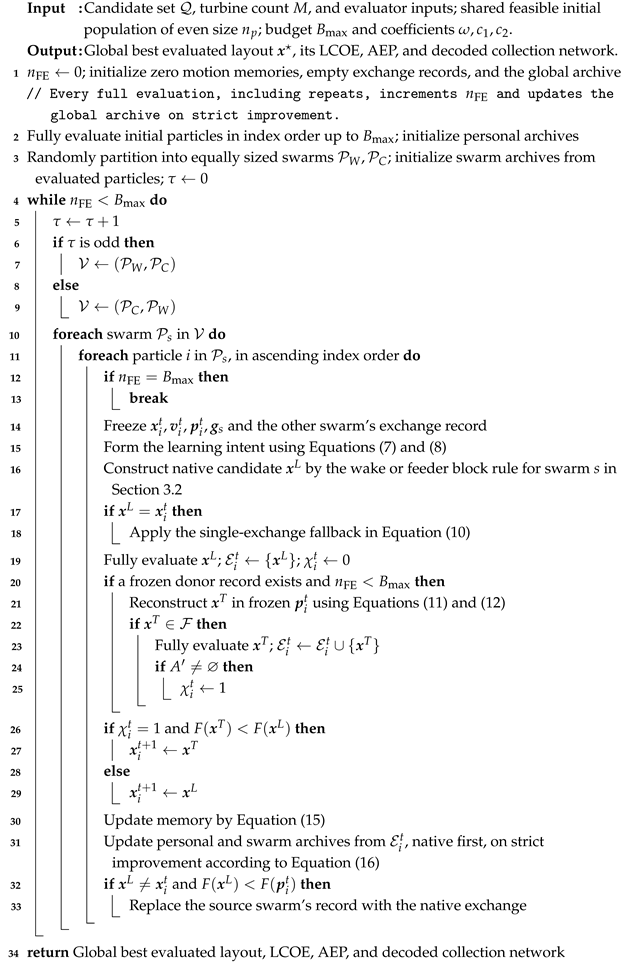
A particle update evaluates one native candidate and may evaluate one recombination. The sole stopping criterion is a budget of complete evaluations, each reconstructing the collection network and computing wake-affected energy and cost. Initialization, both candidate sources, and repeated layouts consume this budget. If only one evaluation remains, it is assigned to the native candidate.
For , let be the number of particle updates and the number of evaluated recombinations. At budget exhaustion,
Equation (17) follows because each post-initialization update uses one or two evaluations, and ensures finite termination. If , the best evaluated initial layout is returned. When , the sole feasible layout is repeatedly evaluated until budget exhaustion. The analytical properties of CSRPSO and their proofs are provided in Appendix A.
Apart from objective evaluations, one particle update requires the following operations. Computing the learning intent and selecting the M largest scores costs . Let m denote the number of intended removals. The minimum-distance pairing of removals and insertions is an assignment problem solved in time, and its lexicographic tie-breaking solves at most further assignments of at most this size. Wake grouping evaluates the indicator in Equation (2) for pairs, collection grouping labels the feeders of the decoded network in time, and checking the spacing of at most m distinct blocks costs . The fallback examines all pairs of unoccupied and occupied sites, and recombination solves one further assignment, with the same tie-breaking, of at most M rows and columns. By comparison, one complete evaluation costs for the wake calculation over A directions and for routing. The search operations therefore grow faster than the evaluation cost when many sites change in one update; Section 5.5 reports the measured wall time.
| Algorithm 1: CSRPSO under a complete-evaluation budget |
 |
4. Experimental Protocol
4.1. Case Inputs and Evaluation Settings
Eight offshore wind-farm cases were evaluated. Figure 1 brings together their site boundaries and wind distributions. Geometry was expressed in metres. Each site boundary was constructed from the supplied turbine coordinates using a boundary shrink factor of 0.3.
Figure 1.
Wind distributions and site boundaries for the eight benchmark cases. Each heatmap shows joint occurrence probabilities in four rows for wind-speed centres and 12 columns for directions. Angles increase clockwise from north: N, E, S, and W correspond to , , , and , respectively. The 48 probabilities sum to 100% for each site, and all heatmaps share a linear color scale from 0% to 15%. The right-hand square shows the site boundary as a dashed outline. Boundaries are scaled independently to comparable visual extents, preserving their shapes and north-up orientation.
All cases used the same power curve for a 4.2 MW turbine with a rotor diameter of 117 m and a hub height of 91.5 m. The cut-in and cut-out speeds were 3 and 25 m/s, respectively. The wind distribution comprised 12 directions at intervals and four speed centres at 5.75, 11.25, 16.75, and 22.25 m/s. Direction angles were converted to radians for evaluation. Seven cases used their supplied joint-frequency tables. For London Array, directional Weibull densities were evaluated at the four speed centres, normalized within each direction, and weighted by the corresponding directional frequencies. The resulting 48-state probabilities summed to one in every case.
Figure 1 pairs the joint wind-state probabilities with the site boundaries. Summing the four speed states within each direction gives the directional marginal. At Zhuhai-Guishan, the direction accounts for 25.52% of occurrence probability, and its 11.25 m/s state accounts for 14.18% of total probability. Shanghai-Lingang has a lower peak directional probability: its most frequent direction, , accounts for 13.12%. The directional marginals govern wake-neighborhood sampling, whereas all 48 joint states enter the AEP evaluation in Equation (3).
Every algorithm used the wake and economic models in Section 2 and the same Sweep routing decoder. The 33 kV collection system used 150, 400, and 800 mm2 cables, priced at 192, 321, and 506 EUR/m, respectively. Their capacities were 5, 8, and 11 turbines at a power factor of 0.95. Sea depth and export-cable length were fixed at 7 m and 0 m, respectively, for these benchmark cases. Project lifetime, discount rate, and the cable-linked cost coefficient followed Section 2.4.
The substation was fixed at the arithmetic mean of the supplied turbine coordinates. This common reference location keeps substation placement outside the comparison of layout search methods; Section 5.3 examines how the comparative results depend on it. A fixed Poisson-disc candidate set was used for each case throughout the comparison. The minimum turbine spacing was 351 m, equal to three rotor diameters, and all distinct candidates satisfied this spacing. Thus, every subset of M candidates satisfied Equation (1), and all six algorithms searched the same admissible site combinations within each case.
Table 1 specifies the turbine count, candidate count, occupancy fraction, and fixed lifetime cost used in each case. Together with the common cable prices and Equations (5) and (6), these costs determine LCOE from a layout’s AEP and collection expenditure. Candidate occupancy ranges from 25.7% at Shanghai-Lingang to 77.2% at Prinses Amalia. The latter has only 18 unoccupied sites, bounding the number of donor targets that can be absent from a receiving personal best; London Array has 352. Section 6 analyzes how candidate occupancy constrains feasible exchanges and receiver-specific reconstruction.
Table 1.
Case parameters. M is the turbine count and N the number of fixed candidate sites. is the layout-independent lifetime cost in Equation (6), including discounted operation and maintenance.
4.2. Algorithms and Evaluation Budget
CSRPSO was compared with the self-adaptive optimal fractional-order guided differential evolution algorithm (SaOFGDE) [43], binary particle swarm optimization (BPSO) [44], AGPSO [23], the dynamic opposite learning-enhanced sparrow search algorithm (DOLSSA) [45], and the teaching-learning-based optimization algorithm with reinforcement learning to adjust phase selection (RLPS-TLBO) [46]. BPSO is displayed as PSO in the figures and tables. For the fixed-cardinality layout representation, the BPSO baseline selects the M candidate sites with the largest velocity components at each position update, thereby preserving turbine count. Each algorithm had 30 independent runs per case, with a population of 30 layouts. Every run terminated after exactly 15,000 complete objective evaluations. Initialization, repeated layouts, opposition candidates, and both native and recombined CSRPSO candidates consumed this common budget. The number of completed generations therefore depended on the evaluations used by each algorithm. Table 2 reports the resulting LCOE comparisons.
Table 2.
LCOE in EUR/kWh under sweep routing: mean and parenthesized sample standard deviation of each run’s best-LCOE solution over 30 runs per algorithm; bold marks the lowest mean per farm. W/T/L counts farms where CSRPSO is significantly better, not significantly different, or significantly worse than the column’s algorithm, marked +, =, and −, respectively. Comparisons use two-sided Wilcoxon signed-rank tests on 30 run pairs per farm at significance level 0.05; direction follows the signed rank sums. Mean ranks compare case-wise mean LCOE across eight farms; lower is better.
Each initial layout selected M distinct sites uniformly without replacement. All six algorithms received the same initial population within each case and repetition, and their random-number generators were reset to the same seed before optimization. Candidate coordinates, wind probabilities, turbine specifications, and evaluator settings remained fixed across algorithms and repetitions.
CSRPSO divided its 30 particles into two swarms of 15 and used and . BPSO used the same inertia and learning coefficients. AGPSO used a learning coefficient of 1.5, a stagnation threshold of seven updates, mutation probability 0.01, and tournament size six. SaOFGDE used best and worst subsets of three individuals, fractional order 0.995, and history weight 0.05; its scale factor was drawn uniformly from , with adaptive selection between crossover-rate intervals and . DOLSSA allocated six discoverers, 21 companions, and three sentinels, with a branch threshold of 0.8. RLPS-TLBO used a Q-learning rate of 0.1, discount factor 0.9, and actions with unit softmax temperature.
The experiments used MATLAB R2025b on a Windows 11 computer with an Intel Core i7-11700 2.5 GHz CPU and 32 GB of RAM. Independent optimization runs were scheduled in parallel under a configured limit of five workers. Wall time was measured separately for each optimizer call, including optimizer initialization, complete evaluations, search-state updates, and progress callbacks at 3000-evaluation intervals. Timing excluded input loading, shared initial-population construction, parallel-pool startup, and subsequent best-layout verification, result export, and plotting. Section 5.5 reports the resulting wall times.
4.3. Performance Measures and Statistical Comparisons
Each run contributed its lowest evaluated LCOE and the AEP, collection-cable cost, and cable lengths of that same layout. Final performance was summarized by the arithmetic mean and sample standard deviation over the 30 runs. Convergence curves used the pointwise mean of best-so-far LCOE at equal evaluation counts, with bands of one sample standard deviation. For the layout comparison, the 30 runs for each algorithm and farm were ordered by final LCOE and then by run index, and the 16th-ranked run was selected as the upper-median representative. Each panel uses that observed run’s saved layout and cable network.
Within each farm, each comparison between CSRPSO and a baseline used 30 run pairs matched by repetition number, seed, and initial population. A two-sided Wilcoxon signed-rank test assessed paired LCOE differences at a significance level of 0.05, using MATLAB’s tie-adjusted normal approximation. After excluding numerically zero differences, absolute differences were ranked with average ranks for ties. Let and be the sums of these ranks for positive and negative CSRPSO-minus-baseline differences, respectively. At , indicated a CSRPSO win and a loss; otherwise the outcome was no significant difference. W/T/L counts aggregate wins, no significant differences, and losses across the eight farms. Separately, mean ranks and the Friedman test used the eight farms as blocks and the six algorithms’ mean LCOE values per block, assigning lower ranks to lower LCOE and average ranks to ties. Effect sizes complement these tests. For each paired comparison, the matched-pairs rank-biserial correlation [47] summarizes the balance of the signed ranks and ranges from to 1. Positive values favor CSRPSO, and when it has the lower LCOE in every non-tied pair. We also report the standardized mean difference , where subscripts C and B denote CSRPSO and the baseline, respectively, and and s are the mean and sample standard deviation of the 30 run-level LCOE values. Positive also favors CSRPSO. For the Friedman test, Kendall’s coefficient of concordance [48], with farms and algorithms, measures agreement in the algorithm rankings across farms.
5. Results
The 1440 runs assess the consistency of CSRPSO’s final LCOE advantage, the evaluation budget required to obtain it, and the engineering changes underlying that advantage.
5.1. Final LCOE and Run-to-Run Variation
CSRPSO achieved the lowest mean LCOE on all eight cases in Table 2, with AGPSO consistently providing the closest competing mean. Figure 2 summarizes these comparisons as the percentage reduction in mean LCOE achieved by CSRPSO relative to each baseline. Against SaOFGDE, PSO, DOLSSA, and RLPS-TLBO, the reductions ranged from 0.753% to 3.663%.
Figure 2.
Percentage reduction in mean LCOE achieved by CSRPSO relative to each baseline, calculated as 100 times the difference between the baseline and CSRPSO means divided by the baseline mean. Means are taken over the 30 runs reported in Table 2, and the color scale is logarithmic. All 40 differences were significant in two-sided Wilcoxon signed-rank tests at the 0.05 level.
Relative to AGPSO, mean LCOE reductions ranged from 0.041% at Prinses Amalia to 0.697% at London Array. Multiplying each mean LCOE difference by the discounted lifetime energy of the CSRPSO layouts gives the corresponding reduction in present-value lifetime cost for the same energy delivery. This reduction ranged from 0.35 million EUR at Prinses Amalia to 17.2 million EUR at London Array, or 0.04–0.72% of , with an equivalent annual amount of 0.025–1.22 million EUR at the 5% discount rate over the 25-year project lifetime. Re-evaluating the final layouts with or cable costs changed by , or with discount rates of 3% and 8%, left CSRPSO with the lowest mean LCOE on all eight farms and mean reductions of 0.041–0.698% relative to AGPSO. This re-evaluation keeps the optimized layouts fixed and does not predict the layouts that re-optimization under each alternative would produce. At Prinses Amalia, 61 of 79 candidates were occupied, leaving 18 unoccupied sites per layout; see Table 1. CSRPSO and AGPSO reached the same best observed LCOE of 0.055678879 EUR/kWh. CSRPSO obtained lower LCOE in 20 of the 30 matched runs, with four ties and six losses.
The paired LCOE tests gave CSRPSO an 8/0/0 win/tie/loss result against each baseline, as summarized in Table 2. Across the 40 comparisons, two-sided signed-rank p-values ranged from to . The Friedman test of case-wise mean LCOE rankings gave with five degrees of freedom and . The rank-biserial correlation was 1.00 in all 32 comparisons with SaOFGDE, PSO, DOLSSA, and RLPS-TLBO, and 0.46–1.00 relative to AGPSO, with the smallest value at Zhuhai-Guishan. Relative to AGPSO, ranged from 0.61 at Prinses Amalia to 4.88 at London Array. The 0.041% mean LCOE reduction at Prinses Amalia thus corresponded to a difference of 0.61 pooled run-to-run standard deviations. Relative to the other four baselines, ranged from 4.37 to 28.90. Kendall’s coefficient of concordance was , indicating high agreement in the algorithm rankings across the eight farms.
The distributional advantage extended beyond the means, as shown in Figure 3. CSRPSO’s first quartile, median, and third quartile were all below AGPSO’s in every case, with lower LCOE in 19–30 matched runs per farm. At London Array, CSRPSO’s worst result, 0.0524787 EUR/kWh, remained below AGPSO’s best result, 0.0525359 EUR/kWh. The two 30-run samples were completely separated despite CSRPSO having a 4.3% larger standard deviation than AGPSO.
Figure 3.
Final best-LCOE distributions in EUR/kWh from 30 independent runs per algorithm and farm. Boxes span the interquartile range (IQR), with median lines; whiskers reach the furthest observations within 1.5 IQR of the box. Open circles mark observations beyond the whiskers. Lower values are better.
CSRPSO also had the smallest standard deviation on six farms. AGPSO was least variable at Egmond aan Zee, and RLPS-TLBO at London Array. At Nysted, CSRPSO’s standard deviation was 56.1% below AGPSO’s, although AGPSO retained the better individual run.
5.2. Search Convergence
CSRPSO had the lowest mean best-so-far LCOE on all eight cases by 7500 evaluations, as shown in Figure 4. At 10,000 evaluations, its mean in every case was below AGPSO’s mean at 15,000 evaluations. It therefore attained a lower mean LCOE with one-third fewer complete evaluations than the closest baseline used for its final result. This comparison charges initialization, native search, and recombination to the same evaluation budget defined in Section 3.5.
Figure 4.
Mean best-so-far LCOE in EUR/kWh over 30 independent runs per algorithm and farm. Shaded bands indicate one sample standard deviation. The horizontal axis counts complete objective evaluations, including initialization and every evaluated candidate.
The contribution of late search differed across farms. Measured from the end of initialization at 30 evaluations, the second half of the budget supplied 24.7% of London’s total mean-LCOE decrease. The corresponding share was 2.3–7.0% across the other seven farms. After 10,000 evaluations, mean LCOE decreased by a further 0.563% at London Array and 0.022% at Prinses Amalia. All 30 London runs also improved during the final 3000 evaluations. The 10,000-evaluation comparison identifies earlier attainment of the baseline’s final quality; the London trajectory shows continued gains from the remaining budget.
To examine other budgets, Table A1 in Appendix B applies the paired comparisons of Section 4.3 to the best-so-far LCOE recorded at 1500, 3000, 5000, 7500, 10,000, and 15,000 evaluations of the same runs. From 5000 evaluations onward, CSRPSO had the lowest mean LCOE on all eight farms and significant advantages over every baseline on every farm. At 3000 evaluations, it had the lowest mean on seven farms; at London Array, PSO had a lower mean, but the difference was not significant. At 1500 evaluations, one-tenth of the budget, PSO was significantly better on the five farms with the most candidate sites, whereas CSRPSO remained significantly better than each of the other four baselines on at least seven farms. For the implemented top-M BPSO baseline, best-so-far LCOE was unchanged between 1500 and 15,000 evaluations in all 240 runs, showing an early plateau. Budgets above 15,000 evaluations were not tested; the continued improvement of all 30 London Array runs during the final 3000 evaluations motivates examining larger budgets for this largest case.
5.3. Energy Production and Collection-System Design
Figure 5 compares energy capture and cable expenditure for the same lowest-LCOE solution from each run. CSRPSO had the highest mean AEP on all eight farms, exceeding AGPSO by 0.039–0.697%, and lower mean cable expenditure on six. The two cable-cost increases occurred at Shanghai-Lingang and Sheringham Shoal.
Figure 5.
AEP and cable costs of each run’s lowest-LCOE layout over 30 independent runs. Left: mean AEP in GWh/year. Right: stacked mean costs of 150, 400, and 800 mm2 cables in million EUR; endpoints and labels give total-cost means. Error bars indicate one sample standard deviation for AEP and total cost. Algorithms appear in the same order, with CSRPSO first; axis ranges vary by farm.
The lifetime-cost weighting explains these two trade-offs between energy and cost relative to AGPSO. In Equation (6), LCOE has an AEP elasticity of at fixed cable expenditure. Its elasticity with respect to cable expenditure at fixed AEP is . Averaged over runs within each case, this cable-dependent share was only 1.05–2.14% for CSRPSO and AGPSO. At Shanghai-Lingang, 1.307% higher mean cable expenditure raised mean lifetime cost by just 0.0246%, alongside 0.304% higher AEP and 0.278% lower mean LCOE. At Sheringham Shoal, the corresponding changes were in cable expenditure, in lifetime cost, in AEP, and in mean LCOE. In both cases, the percentage increase in mean AEP exceeded that in mean lifetime cost.
Conductor allocation also changed the relationship between network length and expenditure. At Egmond aan Zee, CSRPSO’s mean cable length was 24.790 km, versus 24.636 km for AGPSO. Mean cable expenditure was lower, at 6.3438 versus 6.3512 million EUR. Reducing the 400 mm2 length by 0.338 km saved 0.1084 million EUR, exceeding the combined 0.1009 million EUR increase in the other two classes. Capacity-dependent conductor assignment therefore allowed a longer network to cost less under Equation (4).
The source of cable savings relative to AGPSO differed between farms, as shown in Figure 5. At London Array, 800 mm2 cables represented 57.13% of CSRPSO’s mean expenditure, yet the saving came from the 400 mm2 class. Its 0.3119 million EUR reduction outweighed a combined increase of 0.1992 million EUR in the other classes, yielding a net saving of 0.1127 million EUR. At Rødsand II, the net saving was larger, 0.2551 million EUR or 1.408%, and was led by a 0.2805 million EUR reduction in 800 mm2 cables. Figure 6 shows representative complete designs from the run at the upper median LCOE rank for each algorithm and farm.
Figure 6.
Representative layouts from the run at the upper median LCOE rank (16th of 30) for each algorithm and farm. Rows show algorithms, with CSRPSO first, and columns show farms. Layouts within each column share the same spatial scale. Labels give LCOE in EUR/kWh. Black circles denote turbines and red squares substations; cable colors and line styles distinguish 150, 400, and 800 mm2 cross-sections.
Because the substation location strongly affects cable costs, the final layouts of all runs were re-evaluated with the substation displaced from the arithmetic mean by one quarter of the candidate-area extent in each of the four axis directions, with AEP and layout-independent costs unchanged. These displacements increased the mean cable cost of the CSRPSO layouts by 2.6–20.6%. CSRPSO nevertheless retained the lowest mean LCOE on all eight farms for every displacement, with mean reductions of 0.030–0.688% relative to AGPSO and lower LCOE in 18–30 of the 30 matched runs per farm. Two-sided signed-rank tests at the 0.05 level remained significant in 39 or 40 of the 40 comparisons for each displacement; the exceptions were the comparisons with AGPSO at Zhuhai-Guishan under three displacements, with –. These layouts were optimized for the reference location, so the re-evaluation measures the robustness of the comparison rather than the layouts that joint substation optimization would produce.
5.4. Spatial Layouts and Cable-Route Outcomes
Under the common boundary, fixed substation, and Sweep decoder, the selected sites determine both energy capture and the capacity-dependent network.
At London Array, CSRPSO’s representative layout increased AEP from 3296.336 to 3319.419 GWh/year and reduced cable expenditure from 47.4922 to 47.0288 million EUR relative to AGPSO’s representative layout. Total cable length fell from 141.234 to 138.814 km. The 400 mm2 length decreased by 3.044 km, while the 800 mm2 length increased by 1.254 km. The 0.9770 million EUR saving in 400 mm2 cables exceeded the 0.6346 million EUR increase in 800 mm2 cables. Together with 0.700% higher AEP, the 0.976% reduction in cable expenditure yielded 0.716% lower LCOE. This representative design therefore combines improved energy capture with a net saving from conductor allocation.
At Egmond aan Zee, the representative layouts shared 24 of 36 turbine sites. CSRPSO increased AEP by 0.332%, while cable expenditure and network length increased by 13.214% and 5.677%, respectively. The additional 0.7794 million EUR in cable expenditure was dominated by 800 mm2 cables, whose cost increased by 0.7069 million EUR. Under the common lifetime-cost model, total lifetime cost increased by only 0.171%, below the energy gain, so LCOE decreased by 0.160%. This is an energy-led improvement in which the additional collection investment is justified by the associated energy yield.
The representative Shanghai-Lingang layouts show why cable length alone is insufficient to explain collection cost. CSRPSO’s network was 1.854% shorter, but cable expenditure was 2.135% higher. Its 150 mm2 length decreased by 3.042 km, whereas the 400 and 800 mm2 lengths increased by 1.331 and 0.856 km. This shift toward higher-priced cross-sections outweighed the saving in 150 mm2 cables. With 0.277% higher AEP and only 0.039% higher total lifetime cost, the layout nevertheless achieved 0.238% lower LCOE. These representative designs link the economic differences to energy capture and capacity-dependent conductor allocation, consistent with Equation (14).
5.5. Computational Cost
Table 3 reports the mean wall time per run. Each time covers the whole optimizer call, including the 15,000 complete evaluations common to all algorithms; evaluations and search operations were not timed separately. CSRPSO required 1.16–1.68 times the wall time of AGPSO on seven farms. At London Array, the largest case with 175 turbines and 527 candidate sites, its mean run took 252.5 s compared with 58.3 s for AGPSO, a ratio of 4.33. Across all runs, the mean wall time per complete evaluation was 4.0 ms for CSRPSO and 1.7–1.9 ms for the baselines. The additional time remains within minutes per run, but its growth at London Array is consistent with the complexity terms in Section 3.5 that increase faster than the evaluation cost.
Table 3.
Mean wall time per run in seconds over 30 runs, each with 15,000 complete evaluations. The last row gives the mean wall time per complete evaluation over all farms in milliseconds.
5.6. Ablation Study
Four variants were compared with CSRPSO to examine recombination, motion memory, and exchange grouping. w/o recombination omitted personal-best reconstruction and evaluated only the native candidate at each particle update. Intended displacement updated memory using the displacement toward the intended occupancy instead of the executed displacement. w/o memory reset memory to zero after each update, removing the inertial term from the learning intent. Random blocks preserved the seed and size of each wake or feeder block but selected its other members uniformly from the removable turbines.
The comparison covered eight farms with 30 paired runs per farm and a population size of 30. Run k of each variant shared the saved seed, initial population, candidate pool, wind inputs, and sweep-routing setting of CSRPSO run k. Each run supplied its best-so-far LCOE at the selected comparison endpoint. Within each farm, two-sided Wilcoxon signed-rank tests used MATLAB’s tie-adjusted normal approximation at significance level 0.05, excluding numerically zero differences and determining the direction from the signed rank sums. W/T/L counts denote farms where CSRPSO was significantly better, not significantly different, or significantly worse. Mean ranks and the Friedman test used the eight farms as blocks, with the five configurations’ mean LCOE values in each block.
Table 4 compares endpoint LCOE. CSRPSO attained the lowest mean on seven farms and a mean rank of 1.12. The w/o recombination variant had the lowest mean at Prinses Amalia, 0.005% below CSRPSO, but the paired difference was not significant (). The Friedman test detected differences among the five configurations (, four degrees of freedom, ).
Table 4.
LCOE in EUR/kWh at the selected comparison endpoints under sweep routing: mean and parenthesized sample standard deviation over 30 paired runs per farm; bold marks the lowest mean per farm. Marks +, =, and − indicate that CSRPSO is significantly better than, not significantly different from, or significantly worse than the column’s variant (two-sided Wilcoxon signed-rank tests, significance level 0.05). Mean ranks compare case-wise mean LCOE across eight farms; lower is better.
CSRPSO significantly outperformed both intended displacement and w/o memory on all eight farms (W/T/L of 8/0/0 for each). These two contrasts support retaining motion history and updating it from the displacement selected after grouping and candidate competition (Section 3.4). The memory therefore carries changes adopted in complete layouts into subsequent learning.
Against random blocks, CSRPSO achieved a W/T/L result of 7/1/0; Egmond aan Zee was the only farm without a significant difference (). Because this variant preserves each block’s seed and size, the comparison favors using wake and feeder relationships to select its members. Physical grouping thus organizes proposed relocations around directed wake interactions or shared collection branches (Section 3.2).
Against w/o recombination, the result was 4/4/0, with significant differences at Shanghai-Lingang, Sheringham Shoal, Rødsand II, and London Array. The w/o recombination variant was the closest variant to CSRPSO in mean rank (1.88). This pattern supports interpreting cross-swarm reuse as an additional refinement of native search whose observed benefit varies across farms. Its role is to reassess successful exchanges in a receiving personal-best layout, allowing experience from the other physical neighborhood to improve the receiving design through complete economic evaluation (Section 3.3).
The largest relative increase in mean LCOE over CSRPSO occurred at London Array for every variant: 0.322% for w/o recombination, 2.163% for intended displacement, 1.078% for w/o memory, and 1.075% for random blocks, using CSRPSO’s mean as the denominator. Figure 7 shows the paired-run distributions underlying Table 4.
Figure 7.
Best-so-far LCOE distributions in EUR/kWh at the selected comparison endpoints, from 30 paired runs per farm. Boxes span the interquartile range (IQR), with median lines; whiskers reach the furthest observations within 1.5 IQR of the box. Open circles mark observations beyond the whiskers. Lower values are better.
Figure 8 shows the mean best-so-far LCOE trajectories after mapping each run’s convergence history to a common normalized evaluation index ending at 15,000. Each mean curve ends at the corresponding mean in Table 4; the enlarged main panels and full-range insets show the later and overall search trajectories, respectively.
Figure 8.
Mean best-so-far LCOE in EUR/kWh over 30 paired runs per farm. Main panels enlarge normalized indices 5000–15,000 on linear vertical axes; insets show the full 0–15,000 mean trajectories, with dotted vertical lines marking index 5000. Shaded bands in the main panels indicate one sample standard deviation.
6. Discussion and Conclusions
Joint offshore design makes the value of a turbine relocation dependent on the surrounding layout and the collection network. CSRPSO addresses this dependence by treating successful spatial changes as reusable proposals whose value is reassessed in the receiving design. Wake and feeder relationships provide complementary ways to organize search, while complete LCOE evaluation supplies a common selection criterion. Cooperation concerns the construction of candidate changes; the economic decision remains attached to a complete design. This distinction allows physically different search neighborhoods to share experience while accounting for the coupled energy and network consequences of each proposal.
The role of PSO memory follows from this form of cooperation. Reconstruction and candidate competition intervene between an intended move and the layout actually adopted. Recording the selected occupancy displacement keeps subsequent learning tied to the executed trajectory. Under the stated conditions, Appendix A establishes feasibility, bounded and occupancy-consistent memory, and monotone best-so-far values. An accepted recombination thus enters the particle’s subsequent learning through the displacement it actually produces.
The contrast between Prinses Amalia and London Array helps explain why the benefit differs across cases (Table 1, Table 2 and Table 4). At Prinses Amalia, 61 of 79 candidates are occupied, leaving only 18 unoccupied sites per layout. This bounds the number of missing donor targets that reconstruction can introduce. CSRPSO and AGPSO attained the same best observed LCOE, while CSRPSO achieved a 0.041% lower mean and lower first quartile, median, and third quartile. The gain therefore appears in repeated-run quality around a common best observed value. The nonsignificant recombination contrast at this farm () is consistent with limited additional scope for receiver-specific refinement in this high-occupancy case.
London Array has 175 turbines and 527 candidates, leaving 352 unoccupied sites per layout. Here, the two 30-run LCOE ranges were completely separated, and CSRPSO’s mean was 0.697% below AGPSO’s (Figure 3). The decrease from 7500 to 15,000 evaluations accounted for 24.7% of CSRPSO’s total mean-LCOE decrease from the end of initialization at 30 evaluations to 15,000 evaluations, compared with 2.3–7.0% on the other seven farms (Figure 4). All four ablation variants also incurred their largest relative increases in mean LCOE at London Array (Table 4). These observations support an interpretation of sustained refinement among more alternative layouts: the London gain combines better attained economic quality across runs with continued late-search progress. The case contrast thus connects the benefit to both the availability of new relocation targets and the extent to which further search improves complete designs.
Candidate occupancy constrains the feasible exchanges. Under the pairwise-spaced candidate sets used here, the single-turbine exchange neighborhood contains members, while receiver reconstruction can introduce at most missing donor targets (Section 3.3). At full occupancy, , only one layout is feasible and all methods returning it under the common evaluator obtain the same LCOE, so none can have a strict advantage at this endpoint. With M fixed, increasing N lowers occupancy and provides more relocation targets; the economic value of a reconstruction is still determined by Equation (14). The significant paired advantages of CSRPSO over all five baselines held across the observed occupancy range of 25.7–77.2% (Table 1 and Table 2). Because geometry and wind conditions also vary across the eight cases, these results do not isolate an independent occupancy effect. Rankings at other occupancy fractions require budget-matched comparisons using candidate sets at those fractions.
For developers and operators, the practical value of these differences lies in their cost scale and consistency rather than in statistical significance alone. Because offshore projects are capital intensive, the mean LCOE reductions relative to AGPSO correspond to present-value cost reductions of 0.35–17.2 million EUR for the same energy delivery. The advantage was also consistent across runs: the quartiles of CSRPSO’s final LCOE were below those of AGPSO on every farm, and CSRPSO had the smallest standard deviation on six farms, which reduces the risk that a single optimization run returns a comparatively poor design. CSRPSO uses the same candidate sites, evaluator, and evaluation budget as the baselines, so it can replace the search component of an existing layout design workflow without additional modelling inputs. These benefits refer to the modelled LCOE; the selected layouts would still need verification with higher-fidelity wake and electrical models before investment decisions.
The engineering results show why the economic gains do not require uniform reductions in cable expenditure. CSRPSO attained the highest mean AEP on every farm, alongside different collection-cost outcomes; see Figure 5 and Figure 6. The adopted lifetime-cost model gives AEP changes greater proportional influence on LCOE than cable-cost changes. The observed improvements include simultaneous energy and cost gains, energy gains that justify additional cable investment, and savings from changes in conductor allocation. Network length alone misses the load-dependent prices attached to individual branches; the largest expenditure class likewise need not supply the largest saving. Economically preferable designs must therefore be judged by their combined energy production and collection expenditure. Under the fixed-candidate and capacity-constrained Sweep formulation studied here, CSRPSO provides a cooperative search for such complete designs, combining physical exchange structure, contextual economic evaluation, and learning from executed motion.
The wake model is the main simplification of the aerodynamic evaluation. The top-hat Jensen model with centre-point coverage and multiplicative velocity factors does not resolve the radial velocity-deficit profile or partial rotor overlap, whereas Gaussian models represent the radial profile [49], and reviews of wake loss models compare these representations [50]. CSRPSO interacts with the wake model in two places. Candidate selection uses only complete LCOE values, so another wake model can replace Equations (2) and (3) without changing the search operators. The wake swarm uses the indicator in Equation (2) to define directed adjacency; with a continuous deficit model, a threshold on the pairwise velocity deficit could serve the same role. Changing deficit profiles or interaction thresholds can alter wake adjacency and the value of individual relocations, so the size of the advantage reported here may change. Confirming the comparison under a higher-fidelity wake model would require repeating the optimization runs with that model.
The eight cases contain 34 to 175 turbines, whereas future offshore projects may contain several hundred or more. Within this range, the largest case, London Array, showed the largest mean reduction relative to AGPSO, but also the largest increase in wall time, from 58.3 s for AGPSO to 252.5 s for CSRPSO per run (Table 3). This growth is consistent with the complexity analysis in Section 3.5: one complete evaluation scales as , whereas the matching and spacing operations of CSRPSO grow with both the number of intended removals m and the turbine count M. Farms with several hundred to thousands of turbines would therefore require three adaptations. The number of sites changed in one update can be bounded so that the matching cost remains small; spacing checks and wake grouping can be restricted to spatial neighbours, because only nearby candidates violate the spacing limit and wake deficits decay with distance; and the wake calculation within each evaluation can be parallelized across wind directions. A larger farm also enlarges the search space, so the evaluation budget needed for a comparable improvement would have to be established experimentally. These adaptations have not been tested here, and the present results support conclusions only for farms of up to 175 turbines.
A multi-objective extension could retain the occupancy representation, receiver-specific reconstruction, and executed-displacement memory while revising the evaluation and selection of complete designs. Environmental siting restrictions could enter through candidate filtering and additional feasibility checks. Cable-failure and repair scenarios on the decoded network could yield expected unserved energy as a reliability objective. Alternative joint wind distributions could define a common scenario set for all candidate layouts, allowing expected LCOE and expected annual energy shortfall below a prescribed target to be evaluated separately. Personal, swarm, and global archives would retain nondominated designs. Members selected to maintain diversity would supply personal and swarm guidance, with one personal-archive member frozen as the reconstruction context. Dominance and diversity criteria would replace scalar LCOE improvement in candidate competition and archive updating (Equations (13) and (16)), and would also determine which native exchanges are recorded as successful. Equation (14) would still describe the cost–energy balance within each scenario; selection among complete designs would account for the full objective vector.
Author Contributions
Conceptualization, H.Z.; methodology, Z.X., B.Z. and L.Y.; software, Z.X., B.Z. and L.Y.; writing—original draft preparation, Z.X.; writing—review and editing, Z.X., B.Z., L.Y., F.Y. and H.Z.; supervision, H.Z. All authors have read and agreed to the published version of the manuscript.
Funding
This work was supported by the Natural Science Foundation of the Jiangsu Higher Education Institutions of China (Grant No. 23KJA520001), the Jiangsu Provincial University Key Laboratory of Intelligent Multi-source Information Processing and Security, and the Changzhou Sci&Tech Program (Grant No. CJ20250089).
Data Availability Statement
The original data presented in the study are openly available in the CSRPSO-data repository on GitHub at: https://github.com/zbh0528/CSRPSO-data (accessed on 1 November 2026).
Conflicts of Interest
The authors declare no conflict of interest. The funding agencies did not participate in the study design, data collection or analysis, interpretation of the findings, manuscript preparation, or the decision to publish this work.
Appendix A. Analytical Properties
The analysis assumes deterministic finite evaluations, feasible initialization, fixed turbine count, and the stated spacing checks.
Proposition A1
(Cardinality, target retention, and admissibility). Every selected layout remains in . A recombination constructed by Equation (12) contains the donor’s complete target set before the final spacing check.
Proof.
For a physical native block, , , and , hence . A fallback exchange removes one site and inserts a different site, and an unchanged candidate preserves M. For recombination, and , with equal cardinalities. Thus ; targets already in P cannot be removed, and all missing targets are inserted, giving . All candidate coordinates belong to . Native and recombined candidates are selected only after the complete spacing check, and the retained personal best is itself a previously evaluated feasible layout. Induction over particle updates and archive updates proves feasibility. □
Proposition A2
(Uniform nonzero fallback proposals). When fallback is invoked and , each pair in is selected with probability , and the native candidate satisfies and .
Proof.
For an unoccupied candidate a, count its spacing conflicts with S. If there are no conflicts, any can be removed. If there is exactly one conflict, only that conflicting turbine can be removed. Two or more conflicts cannot be eliminated by one removal. The implementation enumerates exactly these admissible pairs and samples one uniformly. Every pair inserts a previously unoccupied site and removes one occupied site, so the native candidate is nonzero and feasible. This property concerns the native proposal before candidate competition. □
Proposition A3
(Balanced, occupancy-consistent motion memory). For and , Equation (15) satisfies, for every update t,
Proof.
For , expanding the recurrence gives
The bracketed vector is a convex combination of binary occupancy vectors: its weights are nonnegative and sum to one. Each component lies in , which proves the sign and unit bounds after subtraction from . Every vector in the combination has component sum M, so the memory has zero component sum. The assertions at follow from zero initialization. □
Equation (A2) identifies memory as current occupancy minus a decaying weighted history. Its inertial contribution to Equation (7) supports occupied sites and opposes vacant sites, with magnitude at most per component; personal- and swarm-best terms provide the remaining preferences.
Proposition A4
(Candidate competition and monotone archives). Equation (13) gives . For , recombination is selected if and only if . Personal, swarm, and global best-so-far objective values are nonincreasing.
Proof.
An ineligible recombination leaves the native candidate selected. An eligible recombination replaces it only for strictly lower LCOE, giving the first assertion. Equation (14), with , proves the equivalence for eligible recombinations. Equation (16) retains the minimum over the frozen personal best and all evaluated candidates. Swarm and global archives apply the same strict-improvement rule over their respective evaluated sets; deterministic evaluation preserves these recorded objective values on repeated visits. □
The selected candidate can be worse than the previous current layout, allowing exploration while the archives retain evaluated gains.
Appendix B. Comparisons at Smaller Evaluation Budgets
Table A1 reports the comparisons summarized in Section 5.2. For each budget, the best-so-far LCOE of every run was taken from its recorded history, and the tests and ranks follow Section 4.3. These are checkpoints from runs configured for 15,000 evaluations rather than independently reconfigured shorter-budget runs, which would change SaOFGDE’s history-activation threshold and DOLSSA’s discoverer update.
Table A1.
Comparisons of best-so-far LCOE at smaller evaluation budgets over the same 30 runs per algorithm and farm. Lowest mean counts the farms on which CSRPSO had the lowest mean LCOE, and Mean rank is its mean rank among the six algorithms. Each W/T/L entry counts farms where CSRPSO is significantly better than, not significantly different from, or significantly worse than the column’s algorithm, using two-sided Wilcoxon signed-rank tests at the 0.05 level.
References
- Hou, P.; Hu, W.; Soltani, M.; Chen, Z. Optimized Placement of Wind Turbines in Large-Scale Offshore Wind Farm Using Particle Swarm Optimization Algorithm. IEEE Trans. Sustain. Energy 2015, 6, 1272–1282. [Google Scholar] [CrossRef] [Scilit]
- Pillai, A.C.; Chick, J.; Johanning, L.; Khorasanchi, M. Offshore wind farm layout optimization using particle swarm optimization. J. Ocean Eng. Mar. Energy 2018, 4, 73–88. [Google Scholar] [CrossRef] [Scilit]
- International Energy Agency. Offshore Wind Outlook 2019; Technical Report; International Energy Agency: Paris, France, 2019. [Google Scholar]
- Keane, A.; Milligan, M.; Dent, C.J.; Hasche, B.; D’Annunzio, C.; Dragoon, K.; Holttinen, H.; Samaan, N.; Söder, L.; O’Malley, M. Capacity Value of Wind Power. IEEE Trans. Power Syst. 2011, 26, 564–572. [Google Scholar] [CrossRef] [Scilit]
- International Renewable Energy Agency. Renewable Power Generation Costs in 2024; Technical Report; International Renewable Energy Agency: Abu Dhabi, United Arab Emirates, 2025. [Google Scholar]
- Nicolosi, C.F.; Tina, G.M. Impacts of Climate Change on the Wind Power Potential of an Offshore Wind Turbine: Three Case Studies from Sicily. In Proceedings of the 2025 AEIT International Annual Conference (AEIT); IEEE: Piscataway, NJ, USA, 2025; pp. 1–6. [Google Scholar] [CrossRef] [Scilit]
- Cazzaro, D.; Koza, D.F.; Pisinger, D. Combined layout and cable optimization of offshore wind farms. Eur. J. Oper. Res. 2023, 311, 301–315. [Google Scholar] [CrossRef] [Scilit]
- Rodrigues, S.; Restrepo, C.; Katsouris, G.; Teixeira Pinto, R.; Soleimanzadeh, M.; Bosman, P.; Bauer, P. A Multi-Objective Optimization Framework for Offshore Wind Farm Layouts and Electric Infrastructures. Energies 2016, 9, 216. [Google Scholar] [CrossRef] [Scilit]
- Pérez-Rúa, J.A.; Cutululis, N.A. A framework for simultaneous design of wind turbines and cable layout in offshore wind. Wind Energy Sci. 2022, 7, 925–942. [Google Scholar] [CrossRef] [Scilit]
- Gong, X.; Kuenzel, S.; Pal, B.C. Optimal Wind Farm Cabling. IEEE Trans. Sustain. Energy 2018, 9, 1126–1136. [Google Scholar] [CrossRef] [Scilit]
- Jin, R.; Hou, P.; Yang, G.; Qi, Y.; Chen, C.; Chen, Z. Cable routing optimization for offshore wind power plants via wind scenarios considering power loss cost model. Appl. Energy 2019, 254, 113719. [Google Scholar] [CrossRef] [Scilit]
- Cazzaro, D.; Fischetti, M.; Fischetti, M. Heuristic algorithms for the Wind Farm Cable Routing problem. Appl. Energy 2020, 278, 115617. [Google Scholar] [CrossRef] [Scilit]
- Shin, S.H.; Song, W.C.; Bae, I.S. Binary Integer Programming-Based Integrated Optimization of Offshore Wind Farm Inter-Array Systems. Energies 2026, 19, 2654. [Google Scholar] [CrossRef] [Scilit]
- Hou, P.; Zhu, J.; Ma, K.; Yang, G.; Hu, W.; Chen, Z. A review of offshore wind farm layout optimization and electrical system design methods. J. Mod. Power Syst. Clean Energy 2019, 7, 975–986. [Google Scholar] [CrossRef] [Scilit]
- Réthoré, P.E.; Fuglsang, P.; Larsen, G.C.; Buhl, T.; Larsen, T.J.; Madsen, H.A. TOPFARM: Multi-fidelity optimization of wind farms. Wind Energy 2014, 17, 1797–1816. [Google Scholar] [CrossRef] [Scilit]
- Tao, S.; Xu, Q.; Feijóo, A.; Zheng, G. Joint Optimization of Wind Turbine Micrositing and Cabling in an Offshore Wind Farm. IEEE Trans. Smart Grid 2021, 12, 834–844. [Google Scholar] [CrossRef] [Scilit]
- He, J.; Ge, M.; Duvnjak Žarković, S.; Li, Z.; Hilber, P. A novel integrated optimization method of micrositing and cable routing for offshore wind farms. Energy 2024, 306, 132443. [Google Scholar] [CrossRef] [Scilit]
- Fischetti, M.; Fischetti, M. Integrated Layout and Cable Routing in Wind Farm Optimal Design. Manag. Sci. 2023, 69, 2147–2164. [Google Scholar] [CrossRef] [Scilit]
- Hu, J.; Xu, J.; Meng, W.; Yang, Q.; Grossmann, I.E. Integrated optimization of layout and cable routing for wind farms: From MINLP to MIQCP formulation and bilevel decomposition method. Comput. Chem. Eng. 2026, 214, 109814. [Google Scholar] [CrossRef] [Scilit]
- Pedersen, J.; Lindner, N.; Rehfeldt, D.; Koch, T. Integrated wind farm design: Optimizing turbine placement and cable routing with wake effects. OR Spectrum 2026. Online First. [Google Scholar] [CrossRef] [Scilit]
- Zhang, D.; Liu, Z.; Liang, Y.; Li, C.; Zhang, J.; Hu, G. Bilevel optimization of non-uniform offshore wind farm layout and cable routing for the refined LCOE using an enhanced PSO. Ocean Eng. 2024, 299, 117244. [Google Scholar] [CrossRef] [Scilit]
- Qi, Y.; Hou, P.; Liu, G.; Jin, R.; Yang, Z.; Yang, G.; Dong, Z. Cable Connection Optimization for Heterogeneous Offshore Wind Farms via a Voronoi Diagram Based Adaptive Particle Swarm Optimization with Local Search. Energies 2021, 14, 644. [Google Scholar] [CrossRef] [Scilit]
- Lei, Z.; Gao, S.; Wang, Y.; Yu, Y.; Guo, L. An adaptive replacement strategy-incorporated particle swarm optimizer for wind farm layout optimization. Energy Convers. Manag. 2022, 269, 116174. [Google Scholar] [CrossRef] [Scilit]
- Zhang, B.; Shao, Y.; Lei, Z.; Zhang, C.; Wang, Y.; Gao, S. A geometry-guided genetic algorithm for integrated offshore wind farm layout and electrical cable routing optimization. Appl. Energy 2026, 415, 127895. [Google Scholar] [CrossRef] [Scilit]
- Wang, Z.; Ding, L.; Wang, X.; Zhang, B. A balance-aware geometric multi-objective evolutionary algorithm for offshore wind farm layout optimization with capacity dependent cable cost evaluation. Energy 2026, 360, 141798. [Google Scholar] [CrossRef] [Scilit]
- Wang, Y.; Liu, H.; Long, H.; Zhang, Z.; Yang, S. Differential Evolution With a New Encoding Mechanism for Optimizing Wind Farm Layout. IEEE Trans. Ind. Inform. 2018, 14, 1040–1054. [Google Scholar] [CrossRef] [Scilit]
- Li, J.; Zhang, Z.; Zheng, T.; Tang, J.; Lei, Z.; Gao, S. Discrete bi-population differential evolution for optimizing complex wind farm layouts in diverse terrains. Energy 2025, 335, 137885. [Google Scholar] [CrossRef] [Scilit]
- Zhang, Z.; Li, J.; Lei, Z.; Zhu, Q.; Cheng, J.; Gao, S. Reinforcement learning-based particle swarm optimization for wind farm layout problems. Energy 2024, 313, 134050. [Google Scholar] [CrossRef] [Scilit]
- Zhang, B.; Shao, Y.; Xu, Z.; Lei, Z.; Luo, X.; Cheng, J.; Gao, S. An Incremental Surrogate-Assisted Differential Evolution for Offshore Wind Farm Layout Optimization. IEEE Trans. Syst. Man Cybern. Syst. 2026. Early Access. [Google Scholar] [CrossRef] [Scilit]
- Thomas, J.J.; Baker, N.F.; Malisani, P.; Quaeghebeur, E.; Sanchez Perez-Moreno, S.; Jasa, J.; Bay, C.; Tilli, F.; Bieniek, D.; Robinson, N.; et al. A comparison of eight optimization methods applied to a wind farm layout optimization problem. Wind Energy Sci. 2023, 8, 865–891. [Google Scholar] [CrossRef] [Scilit]
- Kennedy, J.; Eberhart, R. Particle Swarm Optimization. In Proceedings of the ICNN’95—International Conference on Neural Networks; IEEE: Piscataway, NJ, USA, 1995; Volume 4, pp. 1942–1948. [Google Scholar] [CrossRef] [Scilit]
- Liang, J.J.; Qin, A.K.; Suganthan, P.N.; Baskar, S. Comprehensive Learning Particle Swarm Optimizer for Global Optimization of Multimodal Functions. IEEE Trans. Evol. Comput. 2006, 10, 281–295. [Google Scholar] [CrossRef] [Scilit]
- Lynn, N.; Suganthan, P.N. Heterogeneous Comprehensive Learning Particle Swarm Optimization with Enhanced Exploration and Exploitation. Swarm Evol. Comput. 2015, 24, 11–24. [Google Scholar] [CrossRef] [Scilit]
- Yang, Q.; Zhang, K.X.; Gao, X.D.; Xu, D.D.; Lu, Z.Y.; Jeon, S.W.; Zhang, J. A Dimension Group-Based Comprehensive Elite Learning Swarm Optimizer for Large-Scale Optimization. Mathematics 2022, 10, 1072. [Google Scholar] [CrossRef] [Scilit]
- Czworkowski, C.; Sheppard, J.W. Using Variable Interaction Graphs to Improve Particle Swarm Optimization. In Proceedings of the Genetic and Evolutionary Computation Conference Companion; ACM: New York, NY, USA, 2025; pp. 479–482. [Google Scholar] [CrossRef] [Scilit]
- van den Bergh, F.; Engelbrecht, A.P. A Cooperative Approach to Particle Swarm Optimization. IEEE Trans. Evol. Comput. 2004, 8, 225–239. [Google Scholar] [CrossRef] [Scilit]
- Jensen, N.O. A Note on Wind Generator Interaction; Technical Report Risø-M-2411; Risø National Laboratory: Roskilde, Denmark, 1983. [Google Scholar]
- Gillett, B.E.; Miller, L.R. A Heuristic Algorithm for the Vehicle-Dispatch Problem. Oper. Res. 1974, 22, 340–349. [Google Scholar] [CrossRef] [Scilit]
- Aldersey-Williams, J.; Rubert, T. Levelised cost of energy—A theoretical justification and critical assessment. Energy Policy 2019, 124, 169–179. [Google Scholar] [CrossRef] [Scilit]
- Johnston, B.; Foley, A.; Doran, J.; Littler, T. Levelised cost of energy, A challenge for offshore wind. Renew. Energy 2020, 160, 876–885. [Google Scholar] [CrossRef] [Scilit]
- Chen, W.N.; Zhang, J.; Chung, H.S.H.; Zhong, W.L.; Wu, W.G.; Shi, Y.H. A Novel Set-Based Particle Swarm Optimization Method for Discrete Optimization Problems. IEEE Trans. Evol. Comput. 2010, 14, 278–300. [Google Scholar] [CrossRef] [Scilit]
- Xu, Z.; Zhang, B.; Yu, J.; Yang, L.; Yuan, F.; Gao, S. An Improved Artificial Bee Colony Algorithm with Differential Analysis and Deduplication for Feature Selection. Int. J. Comput. Intell. Syst. 2026, 19, 6. [Google Scholar] [CrossRef] [Scilit]
- Zhang, Y.; Zhang, Z.; Zhong, R.; Yu, J.; Houssein, E.H.; Zhao, J.; Gao, Z. Under complex wind scenarios: Considering large-scale wind turbines in wind farm layout optimization via self-adaptive optimal fractional-order guided differential evolution. Energy 2025, 323, 135866. [Google Scholar] [CrossRef] [Scilit]
- Kennedy, J.; Eberhart, R.C. A discrete binary version of the particle swarm algorithm. In Proceedings of the 1997 IEEE International Conference on Systems, Man, and Cybernetics. Computational Cybernetics and Simulation; IEEE: Piscataway, NJ, USA, 1997; Volume 5, pp. 4104–4108. [Google Scholar] [CrossRef] [Scilit]
- Zhu, Y.; Guo, Y.; Hu, T.; Wu, C.; Zhang, L. Wind Farm Layout Optimization Based on Dynamic Opposite Learning-Enhanced Sparrow Search Algorithm. Int. J. Energy Res. 2024, 2024, 4322211. [Google Scholar] [CrossRef] [Scilit]
- Yu, X.; Zhang, W. A teaching-learning-based optimization algorithm with reinforcement learning to address wind farm layout optimization problem. Appl. Soft Comput. 2024, 151, 111135. [Google Scholar] [CrossRef] [Scilit]
- Kerby, D.S. The Simple Difference Formula: An Approach to Teaching Nonparametric Correlation. Compr. Psychol. 2014, 3, 11.IT.3.1. [Google Scholar] [CrossRef] [Scilit]
- Kendall, M.G.; Babington Smith, B. The Problem of m Rankings. Ann. Math. Stat. 1939, 10, 275–287. [Google Scholar] [CrossRef] [Scilit]
- Bastankhah, M.; Porté-Agel, F. A new analytical model for wind-turbine wakes. Renew. Energy 2014, 70, 116–123. [Google Scholar] [CrossRef] [Scilit]
- Archer, C.L.; Vasel-Be-Hagh, A.; Yan, C.; Wu, S.; Pan, Y.; Brodie, J.F.; Maguire, A.E. Review and evaluation of wake loss models for wind energy applications. Appl. Energy 2018, 226, 1187–1207. [Google Scholar] [CrossRef] [Scilit]
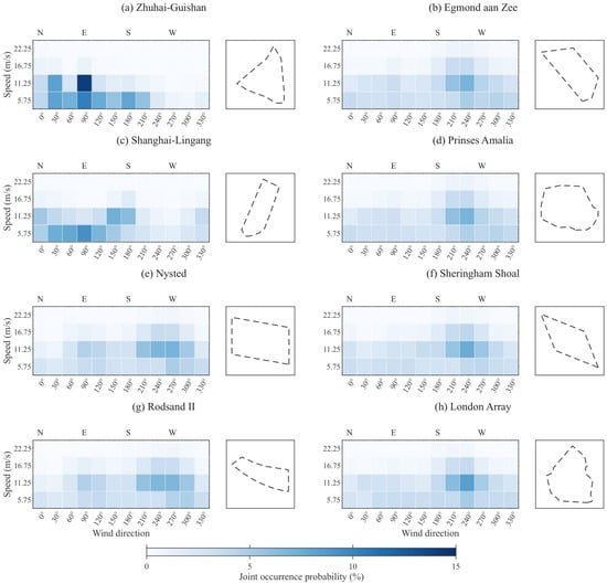
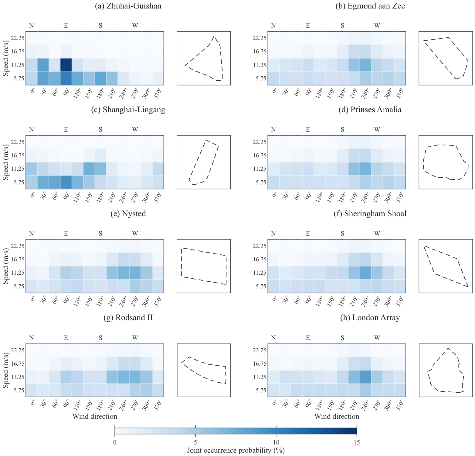
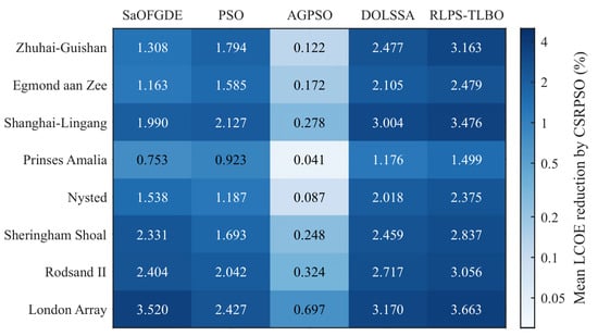
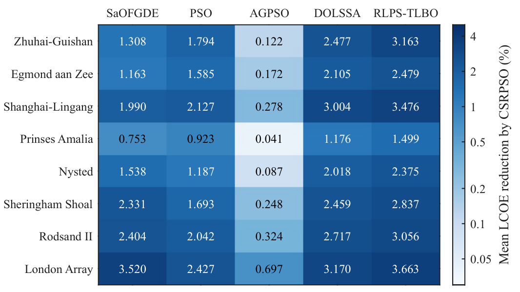
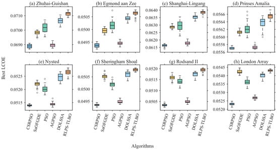
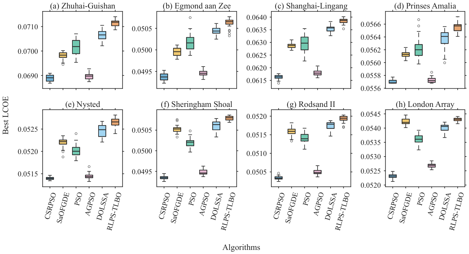
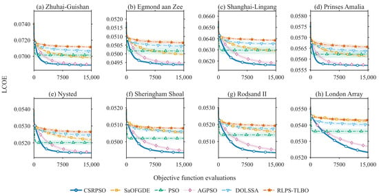
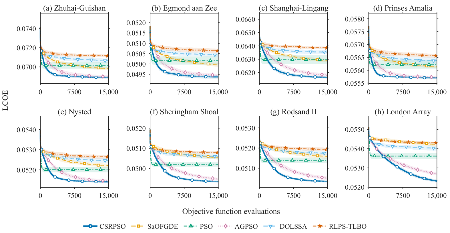
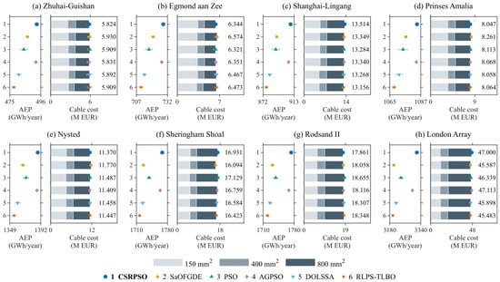
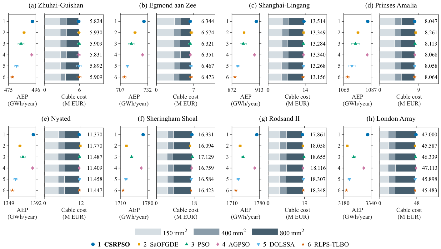
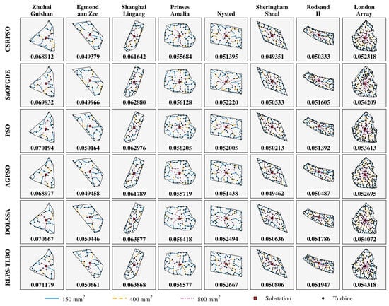
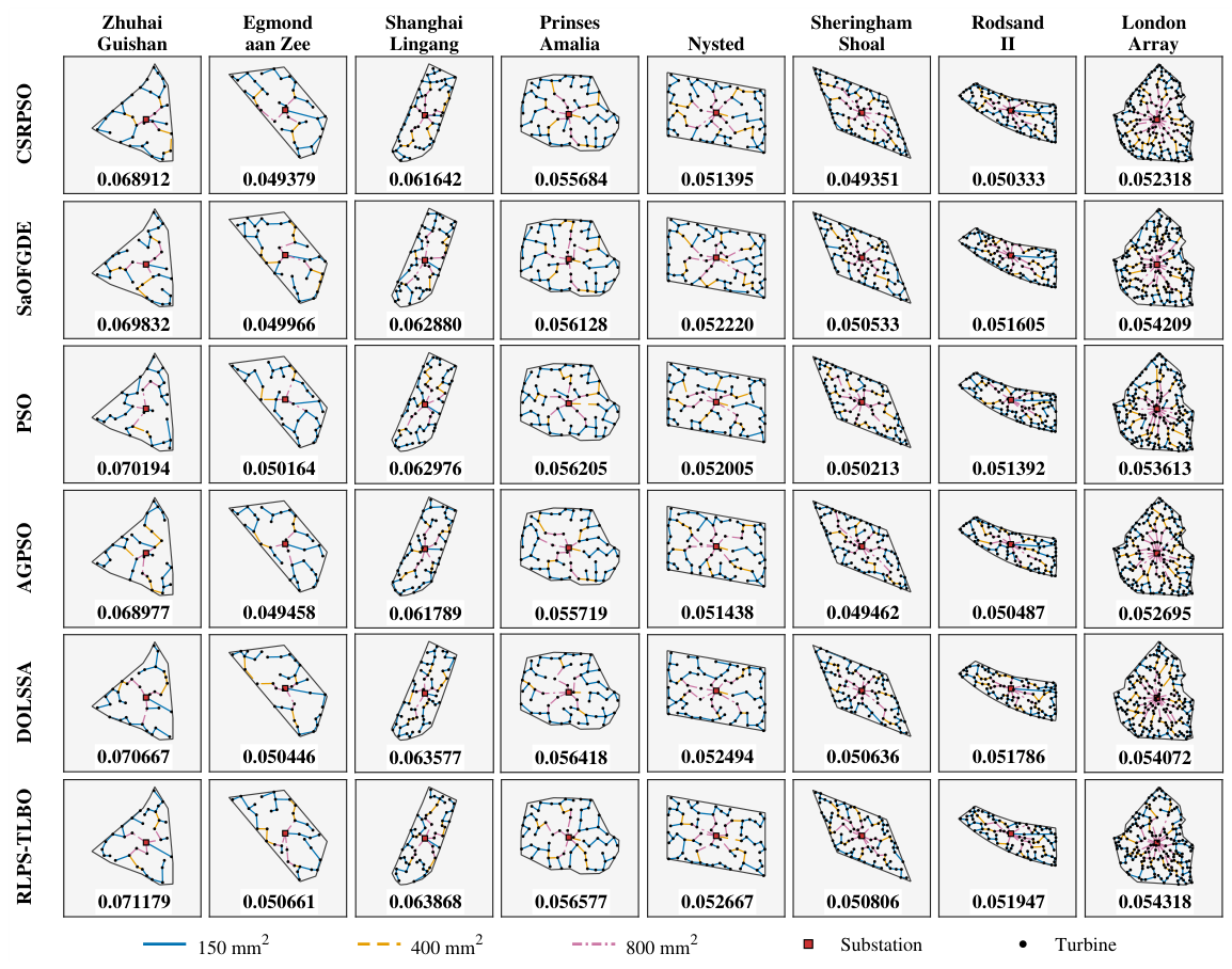
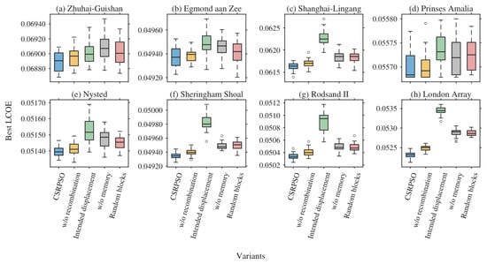
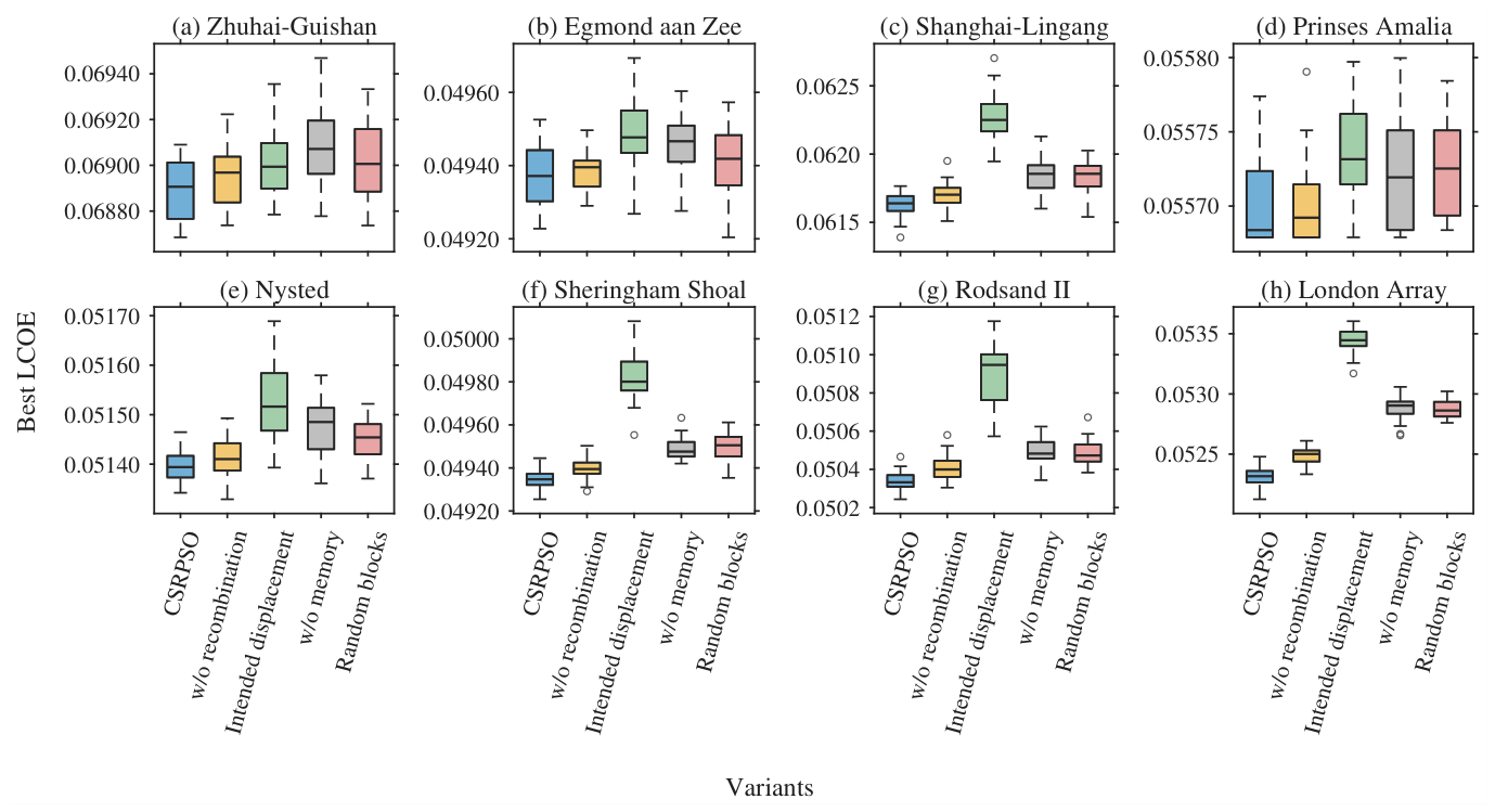
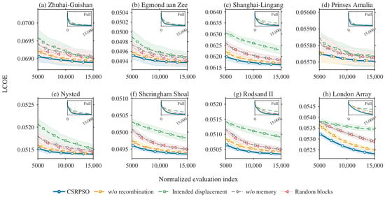
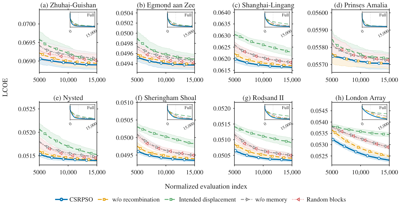

Disclaimer/Publisher’s Note: The statements, opinions and data contained in all publications are solely those of the individual author(s) and contributor(s) and not of MDPI and/or the editor(s). MDPI and/or the editor(s) disclaim responsibility for any injury to people or property resulting from any ideas, methods, instructions or products referred to in the content. |
© 2026 by the authors. Licensee MDPI, Basel, Switzerland. This article is an open access article distributed under the terms and conditions of the Creative Commons Attribution (CC BY) license.