


Abstract
When pumped storage participates in a joint energy and frequency regulation market, competitors’ cost parameters and bidding strategies are not fully observable. The plant must also coordinate pumping and generation schedules across periods and allocate limited capacity between the two markets. The resulting high-dimensional continuous action space and strong physical constraints make bidding optimization under incomplete information sample-inefficient and difficult to converge. This paper therefore proposes a pumped storage bidding strategy that incorporates prior information from forecast electricity prices. First, a directed graph neural network price forecasting model driven by multi-scenario clustering is developed. Historical price data are clustered to decouple operating scenarios, and the directed dependencies between price and its drivers, together with multi-scale temporal features, are learned separately for each scenario to improve day-ahead price forecasting accuracy. Second, the forecast prices are converted into a pumping/generation state prior and a bidding price benchmark prior, thereby constraining the bidding action space. Finally, Bayesian multi-agent reinforcement learning is used to solve the bidding and clearing model. The case study results show that the proposed forecasting model improves the coefficient of determination (R2) from 0.787 to 0.868. Compared with bidding strategies that consider only a single prior, the proposed strategy increases the net revenue of pumped hydro storage by 18.3%.
1. Introduction
Pumped storage hydropower (PSH) combines technological maturity, reliable operation, and large-scale regulation capability, making it a key flexibility resource for the secure operation of modern power systems [1,2]. As electricity spot markets and ancillary service markets continue to develop in China, pumped storage plants have gained an institutional basis for participating independently in coordinated bidding across multiple markets. However, the temporal coupling between pumping and generation and the interaction among revenue streams make their bidding decisions more complex than those of conventional generating units.
When a pumped storage plant participates in the joint day-ahead energy and frequency regulation markets, it must jointly determine its pumping, idle, and generating states; its energy market price quantity offers; and its regulation capacity and mileage offers. Clearing outcomes across these markets are coupled and jointly determine the plant’s final profit [3,4]. Because private information such as competitors’ cost parameters and bidding strategies cannot be fully observed, market clearing outcomes are uncertain and strategy-dependent. Conventional optimization models based on complete-information assumptions therefore cannot accurately represent strategic interactions among market participants. Developing rational bidding decisions from information available before the day-ahead market is thus a critical issue for the market-oriented operation of pumped storage.
Existing research on pumped storage bidding can be divided into two broad categories. The first considers electricity price uncertainty and applies stochastic programming to optimize pumping and generation schedules and bidding strategies by generating price scenarios and maximizing expected profit [5,6,7]. Robust and distributionally robust optimization further use distributional information to obtain decisions that remain effective under extreme-price scenarios [8,9,10]. Although widely applied, these approaches essentially treat the pumped storage plant as a price taker whose bids do not affect market clearing and therefore cannot represent strategic interaction with competitors. Another category uses bilevel optimization or game theoretic models that incorporate bidding decisions and market clearing, and it solves them with metaheuristic algorithms such as PSO and SNMO [11,12,13]. These methods have potential for nonconvex optimization problems and offer useful approaches to pumped hydro storage bidding. However, they typically assume complete information, treating competitors’ private information, such as cost parameters and bidding preferences, as known. In actual markets with incomplete information, the optimality and feasibility of the resulting decisions remain uncertain.
Under incomplete information, reinforcement learning has been introduced into generation company bidding. Studies [14,15,16] applied deep deterministic policy gradient methods to bidding decisions in incomplete information markets. However, the variance of policy gradient estimates tends to increase as the number of agents grows, which may lead to an unstable learning environment and consequently hinder convergence. To further characterize strategic interactions among multiple market participants, studies [17,18,19] adopted multi-agent reinforcement learning algorithms under the centralized training with a decentralized execution framework to simulate the bidding process of generation companies. Such approaches can effectively capture the strategic coupling and dynamic game relationships among competing generation companies. Nevertheless, as the number of market participants increases and their strategies are continuously updated, deterministic policy gradient methods have difficulty in explicitly characterizing the uncertainty in value estimation arising from limited samples, fluctuations in market returns, and changes in competitors’ strategies. This may result in the accumulation of value estimation errors, thereby further impairing the convergence efficiency and training stability of bidding strategies.
To address uncertainty in value estimation, Bayesian reinforcement learning and distributional reinforcement learning have recently provided new approaches to uncertainty modeling. Reference [20] quantified epistemic uncertainty in value estimation by constructing posterior distributions over model parameters, thereby improving exploration efficiency in reinforcement learning. Reference [21] investigated the estimation of epistemic and aleatoric uncertainties in distributional reinforcement learning, providing a basis for probabilistic value representation. Furthermore, Reference [22] proposed a Bayesian multi-agent reinforcement learning method based on distributional value estimation, in which Gaussian priors and Bayesian linear regression were employed to update the posterior distributions of value function parameters, thereby improving the robustness and learning efficiency of multi-agent reinforcement learning. However, these existing methods do not directly address the multi-period operational constraints, cross-market capacity allocation, and coupled bidding decisions associated with pumped storage hydropower participating in joint energy and frequency regulation markets under incomplete information. Therefore, integrating electricity price forecasting priors with Bayesian multi-agent reinforcement learning provides a promising approach to developing bidding strategies for pumped storage hydropower in joint markets.
When competitors’ cost parameters and bids are unavailable, electricity price forecasting can help pumped storage identify price trends, peak and valley periods, and potential arbitrage intervals. Existing forecasting methods include statistical and machine learning approaches. Traditional autoregressive and autoregressive integrated moving average models forecast prices from historical temporal patterns [23,24]. Actual prices, however, are jointly affected by supply, demand, renewable generation, and other factors and are strongly nonlinear, which limits conventional statistical models. Long short-term memory and gated recurrent unit networks have therefore been widely used to capture nonlinear temporal dependence [25,26], but they focus mainly on temporal features and describe complex directional dependencies among price-related variables inadequately. Graph neural networks address this limitation by propagating multi-variate information over graph structures. Reference [27] constructed a multi-dimensional graph model that combines graph attention, multi-head temporal attention, and multi-scale convolution to extract dynamic spatiotemporal dependence. Spatio-Temporal Graph Neural Network (STGNN) [28] and GCN-LSTM [29] further combine graph convolution with recurrent networks. Reference [30] proposed the Multi-variate Time Series Graph Neural Network (MTGNN), which employs adaptive graph learning to capture directed dependencies among variables and integrates graph convolution with temporal convolution for multi-variate time series forecasting. These methods have improved the representation of nonlinear temporal features and multi-variate spatial dependence, but most use a single static graph and cannot adapt to changes in price-driving mechanisms across operating conditions.
To address the challenge that electricity price forecasts cannot be directly converted into operational and bidding decisions for pumped storage plants participating in the joint energy and frequency regulation market under incomplete information, this paper establishes a decision-making framework of “scenario forecasting–dual prior construction–joint market bidding”. The main contributions are summarized as follows:
- (1)
- Methodological innovation. A dual prior construction method tailored for the joint bidding of pumped storage plants is proposed, which overcomes the limitation of existing studies that treat electricity price forecasting and bidding decision-making separately. By integrating the forecasting model based on electricity price scenario clustering and directed graph neural networks with the BMARL-based bidding decision framework, price forecasting information is enabled to guide the bidding decisions of pumped storage plants.
- (2)
- Application innovation. For the scenario where pumped storage plants simultaneously participate in the energy and frequency regulation markets, a bidding and joint clearing model is developed that considers the inter-temporal coupling between pumping and generation, energy storage capacity constraints, and the competition between energy output and frequency regulation capacity. Under the condition that the competitors’ cost functions and bidding strategies are not fully observable, Bayesian multi-agent reinforcement learning is adopted to solve the multi-agent bidding problem. This provides an implementation approach for pumped storage plants to formulate joint market strategies using pre-bidding information.
- (3)
- Performance improvement. Case studies show that the proposed scenario-aware electricity price forecasting model increases the coefficient of determination R2 from 0.787 of the baseline model to 0.868. Compared with strategies using only the operating state prior or only the reference bid prior, adopting both priors improves the net revenue of pumped storage plants by 18.3%, enhancing the overall market profit of the pumped storage facility.
2. Price Prior-Driven Bidding Framework for Pumped Storage
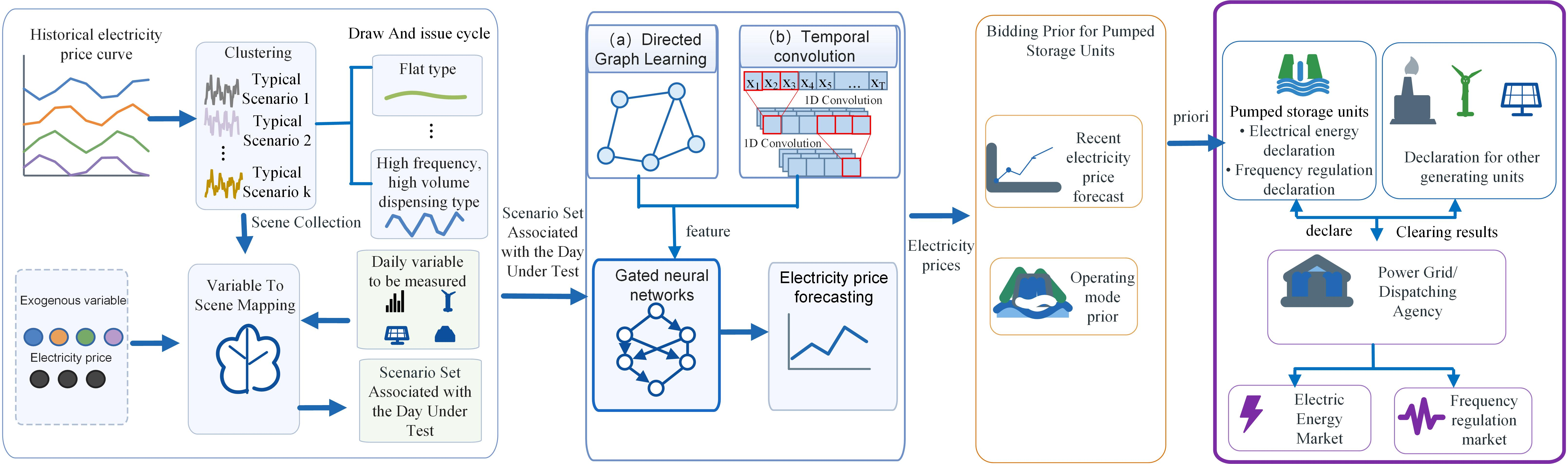
When competitors’ costs and bidding strategies cannot be fully observed, accurate day-ahead price forecasts provide an important basis for PSH bidding. The proposed bidding decision-making framework for PSH participating in the joint market under incomplete information is illustrated in Figure 1.
Figure 1.
Overall framework of price priordriven bidding for pumped storage.
- (1)
- Scenario-clustering directed graph neural network for price forecasting. Historical price curves are first clustered into typical operating scenarios, and a pumping generation cycle prior is established for each scenario. Historical daily load, wind output, photovoltaic output, and fuel prices are then used to train a CatBoost scenario classifier that maps exogenous variables to typical price shapes. Observable target day features are matched to a scenario to form an operating condition specific sample subset. Compared with global training, the decoupled subsets allow the model to learn scenario-specific directed dependence among variables. Multi-scale temporal convolutions extract features at several time granularities, and a gated graph neural network produces the price forecast. This structure suppresses learning noise caused by cross-scenario heterogeneity and improves forecast accuracy.
- (2)
- Construction of bidding priors. The price forecast is converted into two priors used by the bidding model. The operating state prior uses the pumping generation cycle pattern of the target day scenario to define candidate pumping and generating windows; forecast prices within those windows determine the state and specific operating periods, and therefore the direction of energy purchases or sales. The reference price prior uses the forecast price as the baseline purchase or sale offer, narrowing the search space from the full price range to a neighborhood around the baseline.
- (3)
- Joint market bidding and clearing. At the upper level, each participant submits bids to maximize its own profit. The PSH determines its energy market strategy from the bidding priors and submits regulation offers based on opportunity cost; other participants bid according to their costs and operating constraints. At the lower level, the system operator minimizes operating cost through joint energy regulation clearing. The resulting joint market game is solved using BMARL.
3. Day-Ahead Electricity Price Forecasting Using a Scenario-Clustering Directed Graph Neural Network
Considering the differences in the number of peak and valley periods and the dependency relationships among variables under different electricity price scenarios, a scenario-clustering-based directed graph neural network prediction method (MSC-DGNN) is proposed.
3.1. Scenario Clustering Based on Electricity Price Shapes
We use the k-Shape algorithm, which is robust to temporal shifts, so that scenario labels preserve the positions, durations, and spreads of peaks and valleys. A pumping generation cycle pattern is then defined for each scenario.
Assume D historical daily samples, each containing T price periods. The price curve for historical day d is
The k-Shape algorithm is used for clustering, and the number of clusters K is selected using the within-cluster shape loss and average silhouette coefficient. The scenario label for historical day d is defined as
where cd is the scenario label of historical day d; is its normalized price curve; qk is the centroid curve of typical scenario k; and SBD(·) is the shape-based distance used by k-Shape.
The date index set for a typical price scenario k is
Ik = {cd = k∣d ∈ {1, 2, …, D}}
Local extremum detection is applied to each scenario centroid. If scenario k contains Mk peak–valley pairs, its pumping generation cycle pattern is
3.2. Identification of the Target Day Scenario
A CatBoost classifier is trained on historical exogenous features to map exogenous variables to typical price shapes and identify the scenario of the target day.
The exogenous variable vector for historical day d is
where Ld, Wd, and Sd are the load, wind power output, and photovoltaic output on day d, respectively, and Fd is the fuel price. Each historical exogenous vector and the price curve carrying the corresponding scenario label constitute a CatBoost training sample.
ud = [Ld,Wd,Sd,Fd]
The target day exogenous feature vector u0 is input into the trained CatBoost classifier, yielding the probability of matching each typical scenario:
where u0 is the target day exogenous variable vector; fC(⋅) is the CatBoost scenario classifier with parameters θC; and is the output probability vector, where π0,k = P(c0 = k∣u0) is the probability that the target day u0 belongs to scenario k given its exogenous features.
The target day scenario is selected using the maximum predicted probability:
After the target scenario is identified, the sample set corresponding to its historical date indices is extracted:
where is the target scenario sample set; is the set of historical days in the target scenario; di is the date index of its i historical day; and is the exogenous variable matrix for historical day di.
3.3. Directed Dependency Learning and Temporal Feature Extraction
To mitigate the interference of cross-scenario sample heterogeneity with feature learning for the target day scenario, directed graph learning and multi-scale temporal convolution are performed within samples belonging to the target scenario. These two modules are used to learn, respectively, the dependency relationships between electricity prices and their influencing factors from the variable relation dimension and the temporal features from the time dimension.
3.3.1. Directed Dependency Learning
For the target scenario dataset , variables are represented as graph nodes. Price and its drivers are mapped to the node set V = {X1, X2, …, XN}.
To represent scenario-dependent dependency structures, a weighted adjacency matrix W(s) is learned separately for each scenario s. Let D denote the space of directed acyclic graphs (DAGs) over N nodes. The objective is to learn ∈ D that fits the joint distribution ℙ(X) within the scenario.
Writing the weighted adjacency matrix by columns as W = [w1∣w2∣ … ∣wN], the structural equation for variable j is
The weighted adjacency matrix is learned by minimizing a least-squares loss with regularization:
where λ is the sparsity regularization coefficient; the Frobenius norm measures the SEM fitting error; and G(W) is the node graph induced by W. For any W ∈ ℝN×N, a binary adjacency matrix A(W) ∈ {0,1}N×N is constructed, where [A(W)]ij = 1 if wij ≠ 0 and [A(W)]ij = 0 otherwise, thereby obtaining the directed graph G(W). Accordingly, the directed graph G(W) induced by W can be obtained.
After the weighted directed graph for each scenario is obtained, it is incorporated into the gated graph neural network as the structural basis for message passing.
3.3.2. Multi-Scale Temporal Convolution
The directed graph represents dependency topology among variables but not temporal evolution. Load and renewable output affect prices mainly through short-term changes in supply and demand, whereas fuel costs act over longer time scales. Convolution kernels with different lengths and dilation rates are therefore used to extract features at multiple temporal scales.
Dilated convolution enlarges the receptive field without substantially increasing computational cost and can therefore capture temporal dependence more effectively. For a one-dimensional sequence T(X ∈ ℝT) of length T and a convolution kernel L(f1×L ∈ ℝL), the dilated convolution is defined as
where δL is the dilation factor controlling the sampling interval and receptive field. Convolution along the temporal dimension of each variable node sequence extracts local fluctuations, short-term trends, and longer-term dependencies.
For each input sequence, multi-scale convolutions with kernel lengths L2,L3,L6,L7 are applied, and their outputs are concatenated. The multi-scale temporal feature of variable node i is
where L2,L3,L6,L7 are convolution kernel lengths and concat(⋅) denotes concatenation. Let denote the temporal feature matrix. It is used as an input to the graph neural network so that temporal dependence and cross-variable structural dependence are modeled jointly.
3.4. Graph Neural Network Electricity Price Forecasting
Given the learned directed dependency graph G(W) and node temporal features , a gated graph neural network (Gated GNN) integrates variable relationships with temporal features to forecast prices.
Let ei,j denote a directed edge from node vi to node vj. The recurrent message-passing process of the Gated GNN is
where i is a variable node; is its temporal feature extracted by multi-scale convolution; is the initial state before graph propagation; is its hidden state in the preceding layer; is the vector of directed edge weights; and is the message aggregated at node i from other variables.
Equation (13) concatenates the multi-scale temporal feature of each node with a zero vector to construct the initial hidden state. Equation (14) applies the directed adjacency matrix to aggregate hidden states from the preceding layer, yielding the structural information received by node i. Equation (15) then uses the aggregated message as the current input and the preceding layer state as the historical state to update the node representation through a GRU.
The forecast electricity price for target day period t is
where is the transpose of the output layer weight vector, hp,t is the hidden layer state, and bo is the bias of the linear output transformation.
3.5. Pumping and Generating State Selection from Forecast Prices
Given the target day electricity price forecast , the operating state of the pumped storage plant in each period is determined using the quantile method:
where Qτ(⋅) denotes the quantile operator; τL and τH are the lower and upper quantile levels, respectively; and θL and θH are the corresponding forecast price thresholds. Accordingly, the pumped storage operating state is determined as:
4. Bidding and Clearing Model for Pumped Storage in Joint Energy and Regulation Markets
The day-ahead price forecast and the pumping generation operating states are used as prior knowledge for bidding. On this basis, we formulate a bidding and clearing model for PSH participation in the joint energy and frequency regulation markets.
4.1. Pumped Storage Bidding Strategy
4.1.1. Objective Function
The PSH bidding strategy maximizes the plant’s profit:
where T is the number of periods in the scheduling horizon; λE,t, λF,t, λmile,t are the cleared day-ahead energy price, regulation capacity price, and regulation mileage price at time t, respectively; are the cleared generation, pumping consumption, upward regulation capacity, and downward regulation capacity; and αmile is the mileage-to-capacity ratio.
Using the forecast electricity price as a reference, the pumping bid and generating offer in the energy market are expressed as
where β and χ are the pumping and generating bid coefficients, respectively, and where and denote the pumping and generation bids of the pumped storage hydropower unit in the energy market at time t. The opportunity cost of reserving capacity for frequency regulation is calculated as follows:
where denotes the expected opportunity cost of pumped storage hydropower calculated based on the forecasted electricity price. and represent the energy market profits of pumped storage hydropower without and with reserved frequency regulation capacity; and denote the upward and downward frequency regulation capacities reserved at time t, respectively.
4.1.2. Constraints
4.2. Bidding Strategies of Thermal, Wind, and Photovoltaic Units
Thermal and renewable generating units maximize their own profits. Their bidding objective is
where G is the set of conventional generating units; are the energy and regulation market revenues at time t; is the awarded energy; and C is the generation cost. Parameters a,b, and c are fuel cost coefficients for thermal units and maintenance cost coefficients for wind and photovoltaic units. Because wind and photovoltaic units do not provide regulation service, their regulation market revenue is zero.
Cg(P) = agP2 + bgP + cg
4.3. Frequency Regulation Ancillary Service Market
When PSH participates in joint markets, reserving frequency regulation capacity reduces the power available for the energy market, while regulation mileage reflects the value of the regulation service delivered. To examine how these two sources of value affect strategic bidding, this paper constructs a joint market simulation based on the capacity–mileage dual pricing mechanism of the PJM frequency regulation market.
Because spot markets are at different stages of development across China, this paper assumes a mature market in which PSH participate as independent entities in the energy and ancillary services markets and earn revenue through competition. The specific market mechanism is based on the PJM market. Each participant submits a capacity price and a mileage price, and the market operator adjusts the offers using the regulation performance score.
where αmile is the mileage-to-capacity ratio; fs is the regulation performance score; and and are the unadjusted capacity and mileage offers, respectively. Superscript b denotes a submitted offer before adjustment; fs,j is unit j’s regulation performance score; and αmile,j is its mileage-to-capacity ratio. The resulting and are the offer coefficients used in (35).
4.4. Joint Energy Regulation Market Clearing
The joint clearing model minimizes total system expenditure on energy and regulation services:
where G is the set of conventional generating units and g ∈ G indexes a unit. , , and are the cleared energy quantities of unit g, wind generation, and photovoltaic generation, respectively. and are the PSH generating output and pumping consumption. The symbols , πw,t, πs,t, and denote the corresponding energy offer prices, whereas is the pumping purchase bid. , , , and are the cleared upward and downward regulation capacities of conventional units and PSH. The corresponding and terms are their capacity and mileage offer prices after the adjustments defined in Equations (34) and (35).
The clearing model is subject to the following constraints.
- (1)
- Power Balance Constraintwhere is the system demand in period t. This constraint balances scheduled energy quantities; reserved regulation capacity is not counted as scheduled energy output or consumption.
- (2)
- Transmission Flow Constraintswhere k is the set of market participants connected to node k; is the net awarded market power of participant i at time t; is the demand at node k; Gl−k is the power transfer distribution factor from a unit net injection at node k to branch l; is the branch’s maximum allowable transfer; and are the Lagrange multipliers of the maximum reverse and forward flow constraints.
- (3)
- Unit Output and Ramping Constraintswhere and denote the upward and downward ramping limits, respectively.
Regulation Capacity Constraint
The nodal marginal price of each generator can be derived from the joint clearing solution as
where λi is the Lagrange multiplier of the power balance constraint.
5. BMARL-Based Solution for the Bidding Strategy
5.1. BMARL Algorithm Model
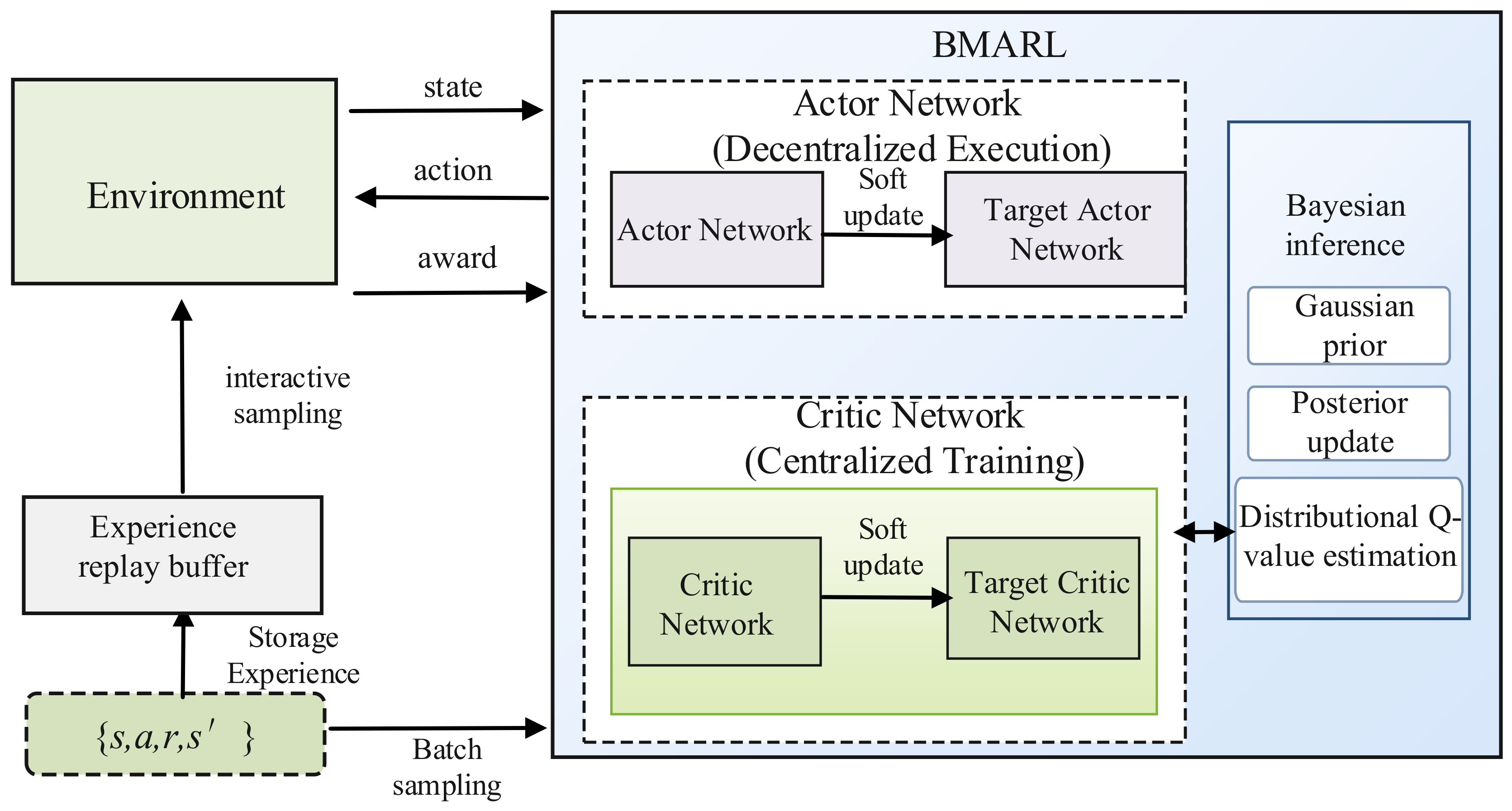
BMARL learns bidding decisions through repeated interaction between market participants and the market environment. Under incomplete information, it uses a Bayesian distribution to estimate uncertainty in the value function and maximum entropy optimization to improve exploration, overcoming the limitations of conventional methods when competitors’ information is unavailable. The model and solution procedure are described below.
- (1)
- Centralized Training and Decentralized Execution
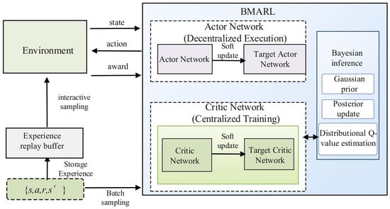
BMARL adopts a Centralized Training and Decentralized Execution (CTDE) framework. During centralized training, the Critic networks use the joint observations and actions of all market participants to learn the interactions among their bidding strategies. During decentralized execution, each agent’s Actor network generates bids using only the local market information available to that agent, enabling bidding decisions under incomplete information.
Let there be N agents in the market. The joint observation and joint action at time t are defined as follows: respectively, they are o = (o1,⋯,oN) and a = (a1,⋯,aN). To capture interactions among agents, an information integrator is introduced into the centralized Critic network to encode the joint observations and actions through feature mapping. The global feature representation for agent i is given by:
where reps and repsa denote the state feature mapping function and the joint state–action feature mapping function, respectively. Their outputs have the same dimensionality.
During policy execution, agent i generates a bidding action from its local observation oi using a stochastic Actor network parameterized ai.
- (2)
- Bayesian Distributional Value Estimation
To mitigate errors arising from deterministic value estimation, BMARL introduces Bayesian linear parameters into the final layer of the Critic network, where the posterior distribution is used to characterize the uncertainty in action value estimates. The action value function of agent i is:
where wi denotes the Bayesian linear weights in the final layer of agent i’s Critic, and Q is its action value function. The vectors o and a represent the joint observations and joint actions of all market participants, respectively. To represent uncertainty in the value function parameters, the final layer weights are assumed to follow a Gaussian distribution wi~(0,σ2I).
A batch of B interaction samples is drawn from the experience replay buffer to construct the feature matrix Fi and the temporal difference target vector yi:
Thus, the Bayesian update of the Critic’s final layer parameter vector becomes a standard Bayesian linear regression problem. The posterior covariance matrix and posterior mean are given by, respectively:
Consequently, after conditioning on the sampled transitions H, the posterior distribution of the final critic layer parameters of agent i is
p(wi∣H) = (μi,Σi)
At the beginning of each training episode, a parameter vector is sampled from the posterior to construct the current critic, whereas the target critic uses the posterior mean. As experience accumulates, posterior covariance contracts gradually, so exploration is stronger during early training and the bidding policy becomes progressively more stable later in training.
- (3)
- Maximum Entropy Policy Evaluation and Network Updates
To prevent premature convergence of bidding policies, BMARL adds entropy regularization to policy evaluation. Agent i samples the next action from the target policy:
where γ is the discount factor and α is the entropy regularization coefficient. The target critic’s posterior mean evaluates the next action, while the entropy term maintains exploration in the continuous action space.
Using the temporal difference targets, the Critic’s feature extraction network is updated by minimizing the value loss:
The Actor network is updated by minimizing the entropy regularized policy loss:
Here, the action value is provided by the Bayesian Critic, so uncertainty in the value estimate is incorporated into the policy update. To improve training stability, target Actor and Critic networks are introduced, and their parameters are updated by soft updates:
where τ is the target network soft update coefficient.
By combining Bayesian value estimation with maximum entropy policy optimization, BMARL coordinates bidding revenue and policy exploration under incomplete market information, improving the training stability of continuous bidding decisions.
5.2. Model Solution
The bidding and market clearing models are solved using BMARL, where each market participant is modeled as an agent. The state information consists of the forecasted electricity price, prior information on pumping/generating states, and the bids of other participants; the agents’ bidding decisions are defined as actions; the market clearing results, including cleared quantities and prices, are used as environmental feedback; and the net profit of each participant is taken as the reward. The BMARL-based solution process is shown in Figure 2.
Figure 2.
Model solution process.
5.2.1. State Space
The state space S consists of the local observations of all agents and represents historical market information and the current operating condition:
where is the electricity price forecast produced by the MSC-DGNN model; Dt−1, Dt are the system loads in the previous and current periods, respectively; are the clearing price and awarded energy quantity in the previous period, respectively; and Vt is the reservoir storage of the pumped storage plant.
5.2.2. Action Space
The action space ai is the continuous price quantity decision of each agent and is defined as
where is agent i’s energy market offer price for the next period. For the pumped storage unit, this offer is adjusted based on the electricity price forecast produced by MSC-DGNN. is the energy quantity offered by agent i; , and are agent i’s regulation capacity offer price, offered regulation capacity, and regulation mileage offer price, respectively.
5.2.3. Reward
The reward ri of agent i is the net profit it earns by participating in the joint energy and regulation market.
The specific steps of the BMARL algorithm are provided in Appendix A.
6. Case Study
6.1. Parameter Settings
Historical market data for a region from 1 January 2019 to 31 December 2023 are used. Each day contains 24 periods, and the features for each period include electricity price, load, coal price, wind generation, and photovoltaic generation. The historical market data from 2019 to 2023 are divided chronologically into training, validation, and test sets at a 6:2:2 ratio. All data preprocessing is performed after the split. In particular, k-Shape clustering, feature selection, and directed graph construction use only the training set. The validation set is used to select hyperparameters and adjust training, while the test set is reserved for independent evaluation of forecasting performance and is not used to update any model parameters. Simulations are implemented in Python 3.8 using PyCharm 2.0.1. MAE, RMSE, MAPE, and R2 are used to evaluate price forecasting; the corresponding evaluation metrics are defined in Equations (A1)–(A5) in the Appendix B.
The parameters of the generating units in the system are provided in Appendix C Table A1, while the load demand and renewable energy generation forecasts for the test day are shown in Appendix C Figure A1. The relevant parameters of the BMARL algorithm are listed in Appendix D Table A2.
6.2. Results and Discussion
6.2.1. Scenario Clustering and Feature Contribution Analysis
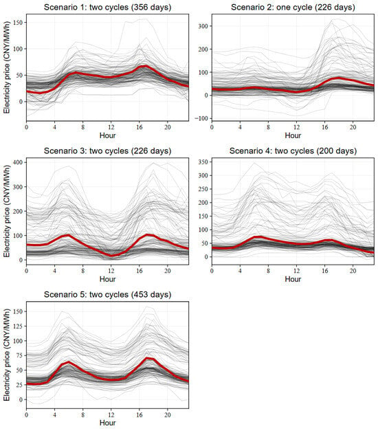
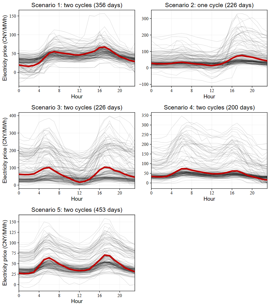
Figure 3 shows five typical day-ahead electricity price scenarios obtained by k-Shape clustering. The gray lines represent individual historical daily electricity price curves within each scenario, while the red line represents the corresponding cluster centroid obtained by k-Shape clustering. Scenarios 1, 3, 4, and 5 each contain two valley-to-peak intervals and can therefore support two pumping generation cycles. Nevertheless, their peak and valley positions, relative spreads between the two cycles, and durations differ, indicating that scenarios with the same number of cycles do not necessarily provide identical operating conditions or arbitrage opportunities. In Scenario 2, the main price spread is concentrated in a single valley-to-peak interval, corresponding to one pumping generation cycle.
Figure 3.
Clustering results for historical electricity price curves.
A scenario-specific pumping generation cycle prior is therefore constructed. In addition to the number of cycles, the prior retains the location, duration, and spread structure of peaks and valleys, thereby supporting subsequent operating state decisions. Scenario partitioning also provides decoupled sample subsets for price forecasting.
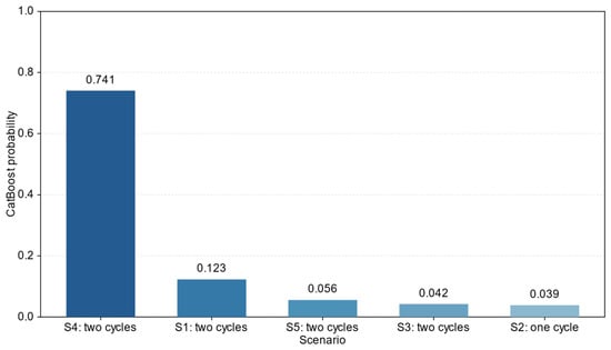
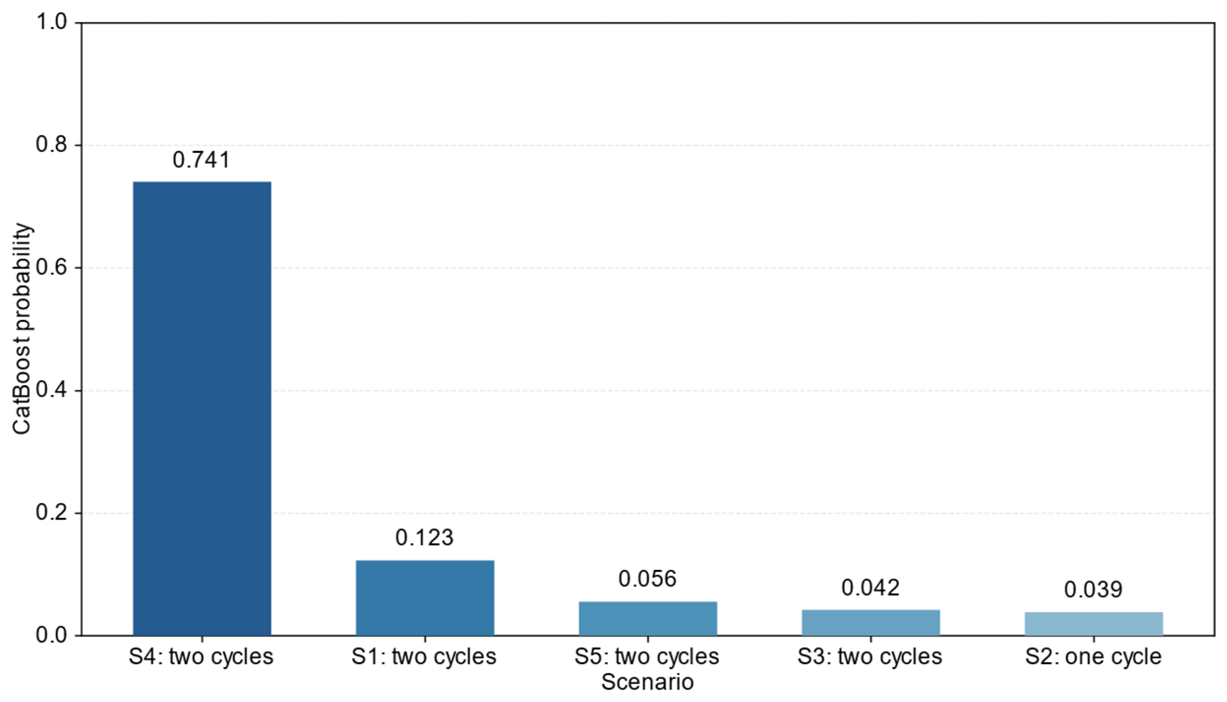
Figure 4 shows the probabilities predicted by the CatBoost model for the target day’s price scenarios using exogenous forecast information available before the day-ahead market. The predicted probability of Scenario 4 is 0.741, substantially higher than the alternatives; the target day is therefore assigned to Scenario 4 under the maximum probability criterion, and the corresponding training samples are selected for electricity price forecasting.
Figure 4.
Scenario matching for the target day.
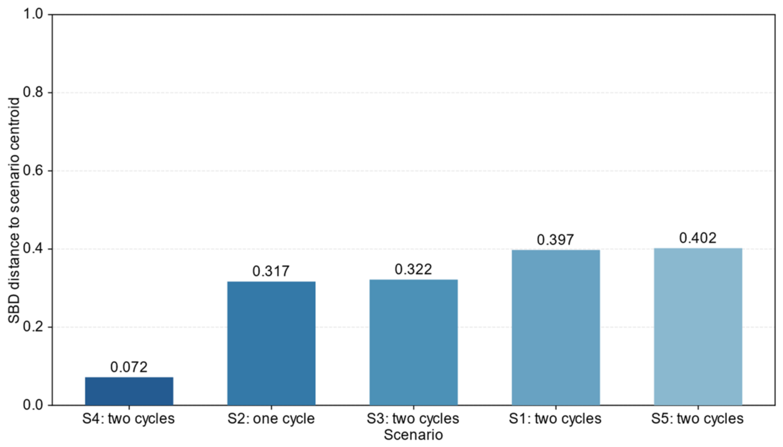
Figure 5 further shows the k-Shape distances between the target day’s actual electricity prices and the centroids of the typical scenarios. These distances are calculated only after the actual prices become available. They serve to validate the day-ahead scenario classification retrospectively and are not used for scenario selection, network parameter updates, or generation of the pumping and generation state prior. This separation of advance scenario prediction from retrospective price pattern validation prevents the target day’s actual prices from entering the day-ahead forecasting process.
Figure 5.
k-Shape distances from the actual target day price curve to each scenario centroid.
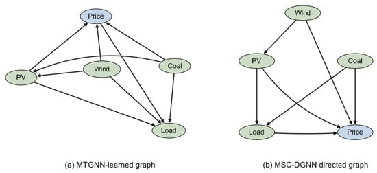
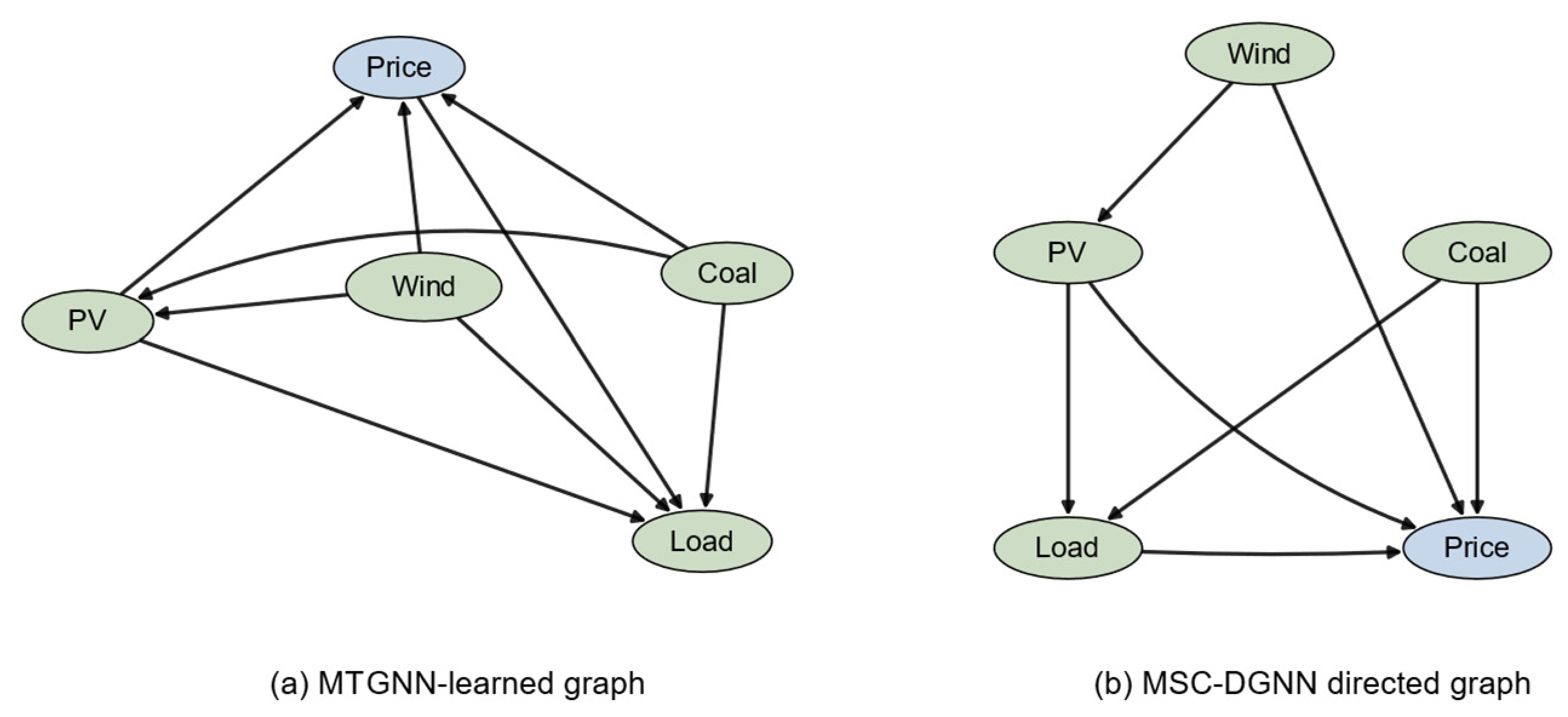
Figure 6 compares the variable correlation structures learned by MSC-DGNN and MTGNN. Unlike MTGNN, which constructs variable relationships mainly based on node feature similarity, MSC-DGNN adopts directed graph structure learning to explicitly characterize the directional dependencies between electricity price and variables such as wind power output, photovoltaic output, load, and coal price. It can be observed that multiple directed edges point to the electricity price node, indicating that the model identifies statistical correlations between several exogenous variables and electricity price during electricity price forecasting. These directed relationships reflect the feature dependency structure learned by the model. By introducing a directed and sparse graph structure, MSC-DGNN constrains the information propagation paths among variables and provides a more targeted feature aggregation architecture for graph neural networks, so as to improve electricity price forecasting performance.
Figure 6.
Directed dependency graphs learned by MSC-DGNN and MTGNN.
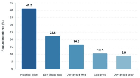
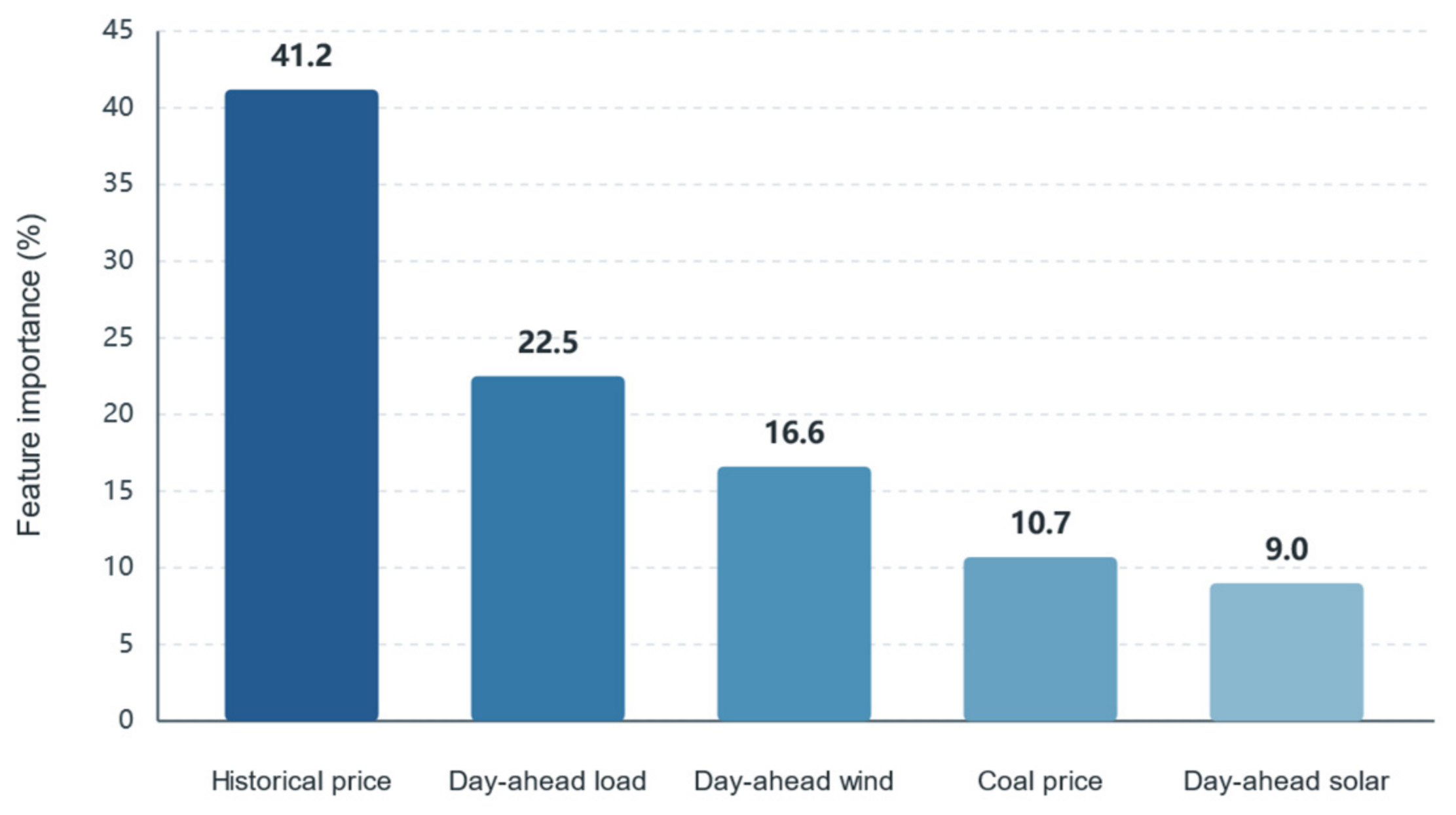
Figure 7 presents the feature importance analysis used to quantify the contribution of each input variable to the day-ahead electricity price forecasts produced by MSC-DGNN. Historical price and load account for 41.2% and 22.5%, respectively, indicating strong dependence on load and prices from comparable scenarios. Wind and photovoltaic forecasts contribute 16.6% and 9.0%, showing that renewable output affects price through net load and the supply demand balance. Coal price contributes 10.7%, reflecting its indirect effect through the marginal costs of thermal generation. These results are consistent with electricity price formation and support the selected MSC-DGNN inputs.
Figure 7.
Feature importance for electricity price forecasting.
6.2.2. Electricity Price Forecasting Results
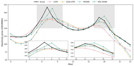
MSC-DGNN is compared with LSTM, GCN-LSTM, and MTGNN. LSTM extracts temporal dependence from the price series; GCN-LSTM jointly models multi-variate relations and temporal features through graph convolution and recurrence; and MTGNN identifies inter-variable associations through adaptive graph learning. To ensure a fair comparison, LSTM, GCN-LSTM, MTGNN, and MSC-DGNN use the same chronological data split and evaluation metrics. When forecasting the target day, each model uses only information available before its forecast is issued.
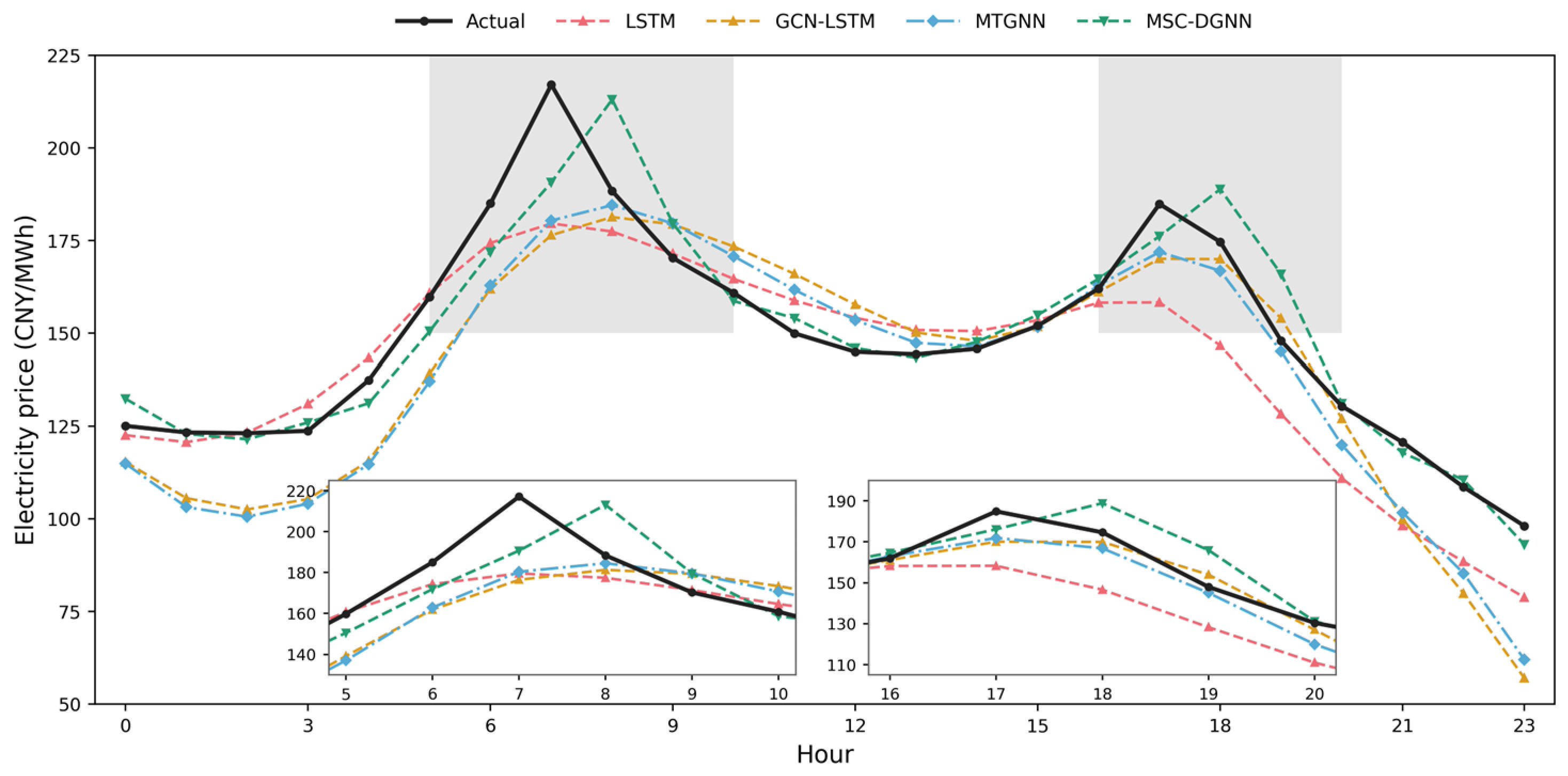
Figure 8.
Dayahead electricity price forecasting results.
Table 1.
Forecasting error metrics for different models.
As shown in Figure 8, all four forecasts reproduce the overall trend of the actual price curve, but MSC-DGNN is consistently closest to the observations. LSTM exhibits comparatively large deviations during the morning peak at 08:00–10:00 and the evening period at 21:00–23:00, while GCN-LSTM and MTGNN show clear errors during the morning peak.
Table 1 shows that MSC-DGNN outperforms all benchmark models for every metric. Relative to the second-best MTGNN model, MSC-DGNN reduces MAE from 14.060 to 6.993, RMSE from 15.192 to 10.073, and MAPE from 10.182% to 4.277%, while increasing R2 from 0.787 to 0.868. These results demonstrate the higher forecasting accuracy of MSC-DGNN.
The improvement arises because MSC-DGNN constructs a scenario-specific training subset for each typical price pattern. The model can therefore learn variable dependencies and temporal features from internally consistent samples while avoiding cross-scenario interference, which is particularly beneficial during peak price periods.
To evaluate the reproducibility and training stability of the forecasting models, each model was independently retrained three times using different random seeds. Specifically, one month of data in 2023 was selected as the test set, while the remaining data were chronologically divided into training and validation sets. The results are reported in Table 2.
Table 2.
Electricity price forecasting performance of different models over three independent runs.
As shown in Table 2, MSC-DGNN consistently achieves the best forecasting performance in terms of all four evaluation metrics across the three independent runs. The standard deviations of MSC-DGNN are 0.299 for MAE, 0.371 for RMSE, and 0.012 for R2, indicating relatively limited variation in these evaluation metrics across independent training runs. Although some variability remains in MAPE, MSC-DGNN maintains a substantially lower mean MAPE than the baseline models. These results suggest that the forecasting improvement is not attributable solely to a particular model initialization and that MSC-DGNN achieves relatively stable predictive performance under repeated training.
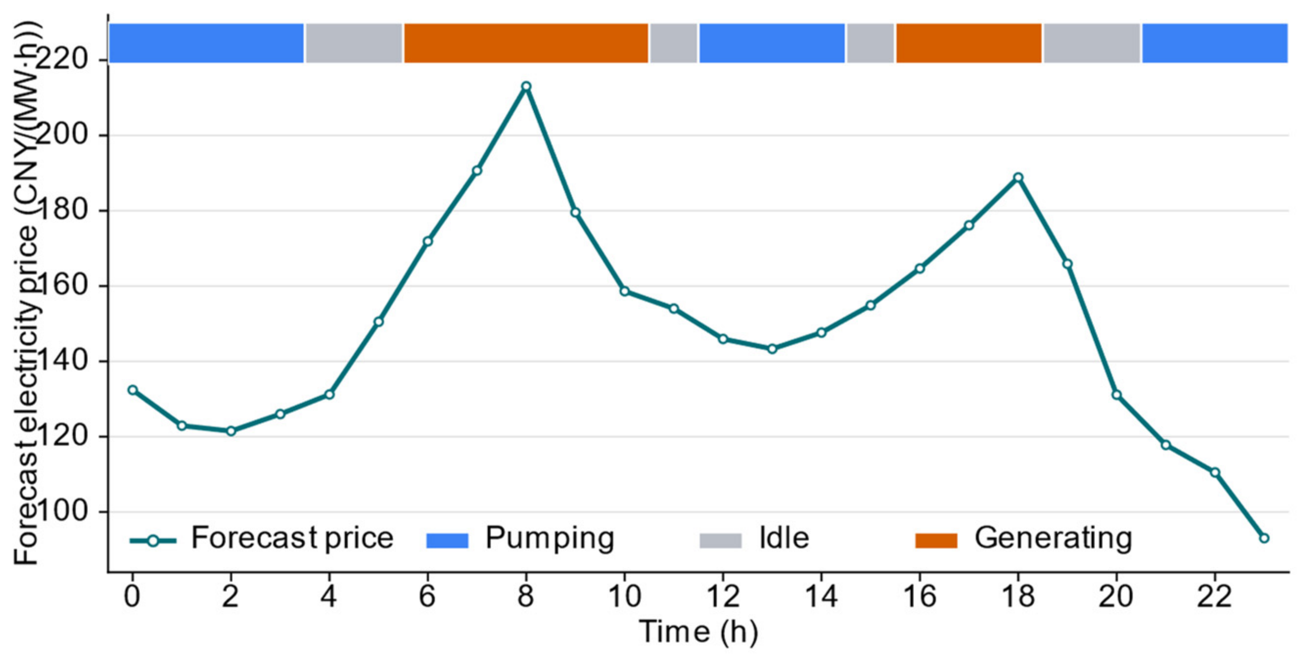
6.2.3. Selection of Pumping and Generating States
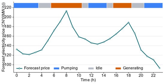
The target day is identified as Scenario 4, which contains two pumping generation cycles. Figure 9 presents the pumping and generating states determined within the candidate operating windows based on the forecast electricity prices. The target day has two pronounced high-price windows, with a higher midday peak than the evening peak. Generating priors are assigned to 06:00–10:00 and 16:00–18:00 to capture high-price revenues, while pumping priors are assigned to low-price periods including 00:00–03:00, 12:00–14:00, and 21:00–23:00.
Figure 9.
Selected pumping and generating states.
6.2.4. Algorithm Performance
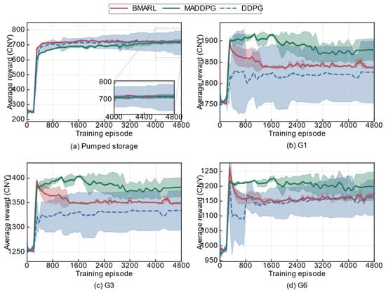
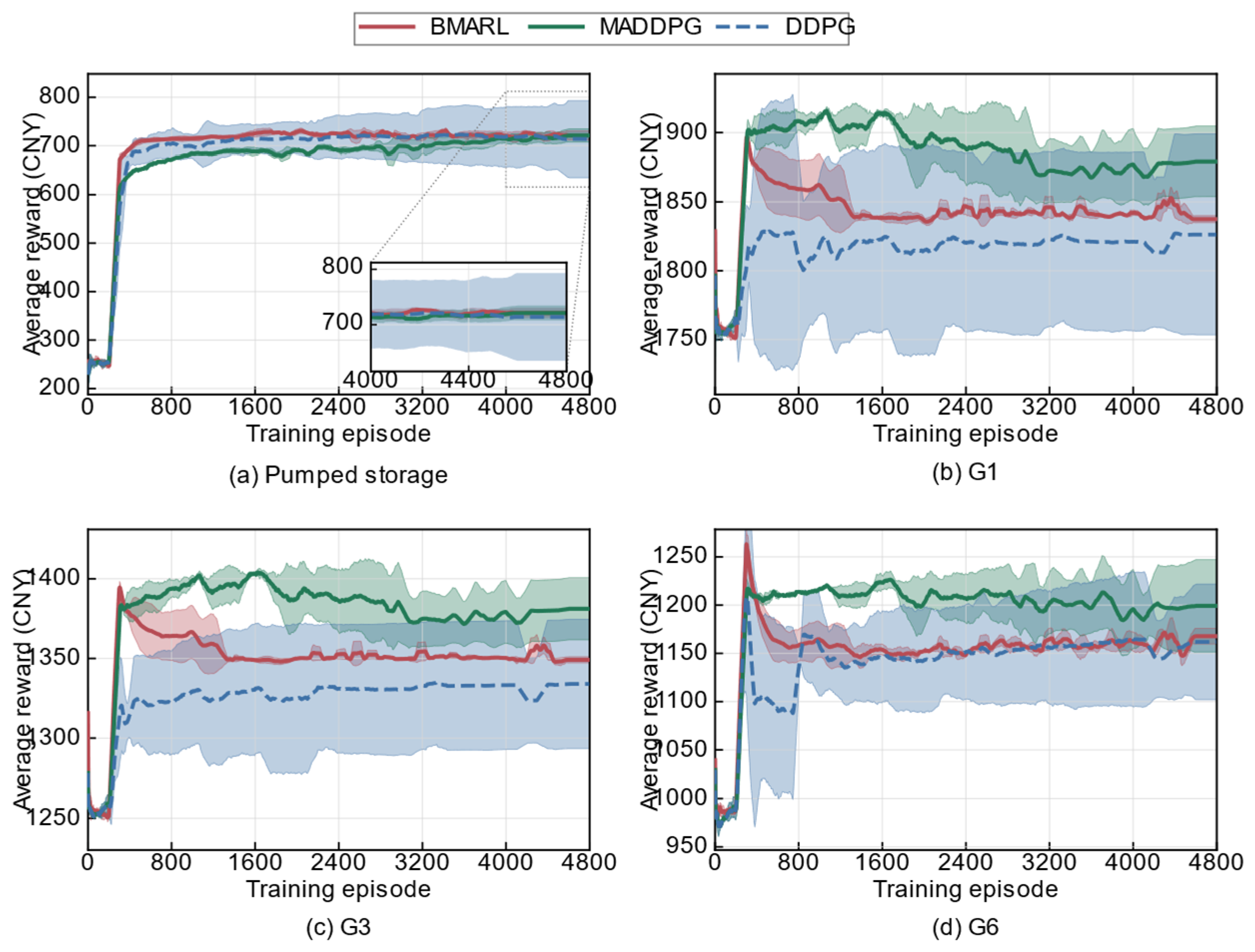
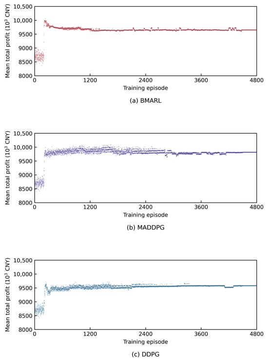
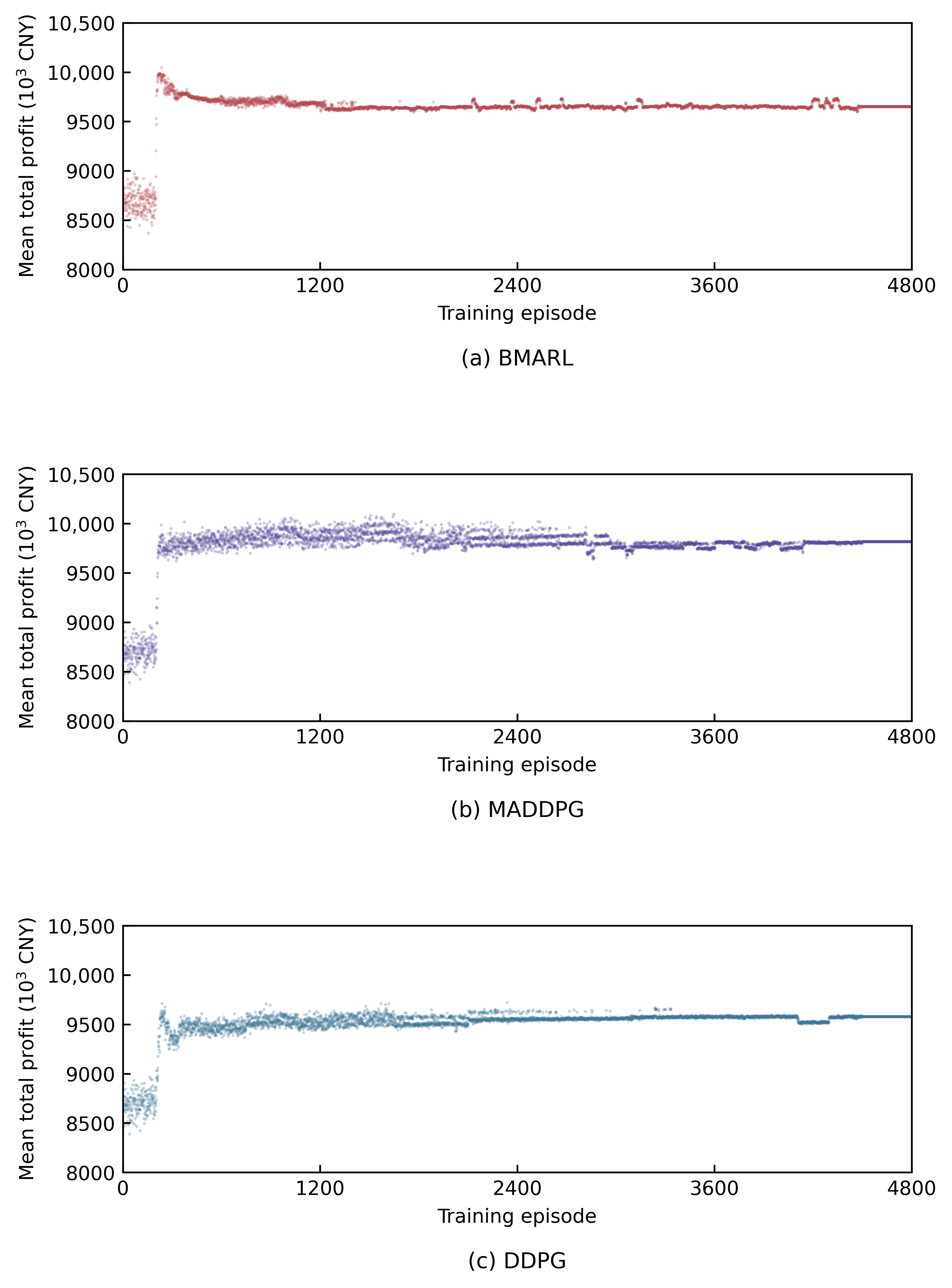
To evaluate the performance of BMARL, comparative experiments are conducted against DDPG and MADDPG under identical model hyperparameters. Each algorithm is independently executed five times, and sliding average rewards are used to evaluate convergence behavior and training stability. Figure 10 presents the episodic reward curves of representative market participants, while Figure 11 illustrates the evolution of the total market profit during training.
Figure 10.
Convergence of episodic rewards for representative market participants under different algorithms.
Figure 11.
Curve of total revenue iteration times variation.
BMARL, MADDPG, and DDPG are compared in terms of reward level, convergence speed, and training stability. Figure 10a–d presents episodic rewards for the pumped storage plant and thermal units G1, G3, and G6. Solid curves represent mean rewards over repeated experiments, and shaded bands indicate variability.
DDPG models each decision-maker as a single agent. When multiple participants update their policies simultaneously, the resulting environment is strongly non-stationary and the reward curves fluctuate considerably. Units G3 and G6 reach stable states only after approximately 1564 and 826 episodes, respectively, and the pumped storage plant’s final mean reward is approximately 713.91.
By introducing the joint states and actions of all participants into a centralized critic, MADDPG represents strategic interactions more fully. The representative thermal units achieve higher final rewards, but the pumped storage policy requires substantially more episodes to become stable. Thus, although a deterministic centralized value function can increase the profit of some participants, its estimates still fluctuate under the combined effects of intertemporal pumped storage constraints and simultaneous policy changes.
BMARL achieves a better balance among reward, convergence speed, and stability. Units G1, G3, and G6 stabilize after 253, 263, and 258 episodes, respectively, requiring approximately 11.6–13.2% fewer training episodes than MADDPG. Pumped storage converges after approximately 420 episodes. Its final BMARL reward is 721.13, exceeding the DDPG result. Overall, BMARL achieves the highest rewards with fewer training episodes and substantially lower reward variability.
Figure 11 further compares the evolution of the total market profit over training episodes under the three algorithms. As shown in Figure 11a, BMARL achieves a rapid increase in total profit during the initial training stage and subsequently maintains a relatively stable level with limited fluctuations. In contrast, MADDPG exhibits more pronounced profit fluctuations during the early and intermediate training stages. DDPG shows a slower adjustment process and eventually converges to a lower profit level. These results indicate that BMARL achieves a favorable balance between convergence efficiency and training stability. Combined with the individual reward curves of market participants in Figure 10, the results further suggest that Bayesian value estimation and entropy-regularized policy optimization help mitigate the training instability caused by simultaneous policy updates among multiple agents under incomplete information. By incorporating uncertainty into value estimation, BMARL enables market participants to learn relatively stable bidding strategies more efficiently, thereby improving the convergence performance of the multi-agent bidding process.
6.2.5. Comparison of Bidding Strategies
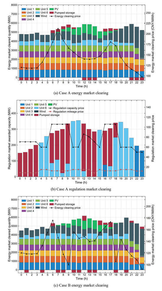
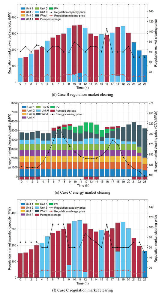
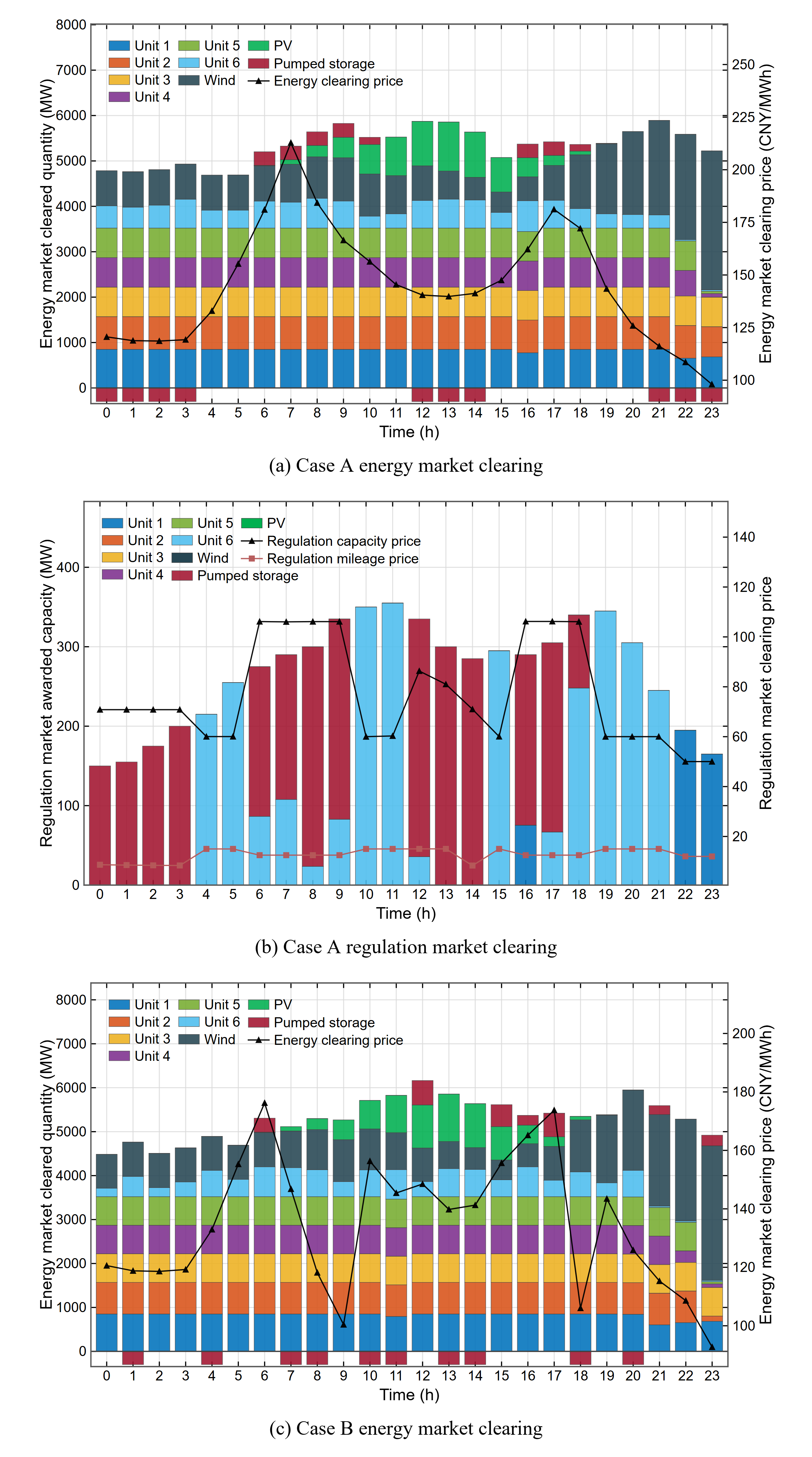
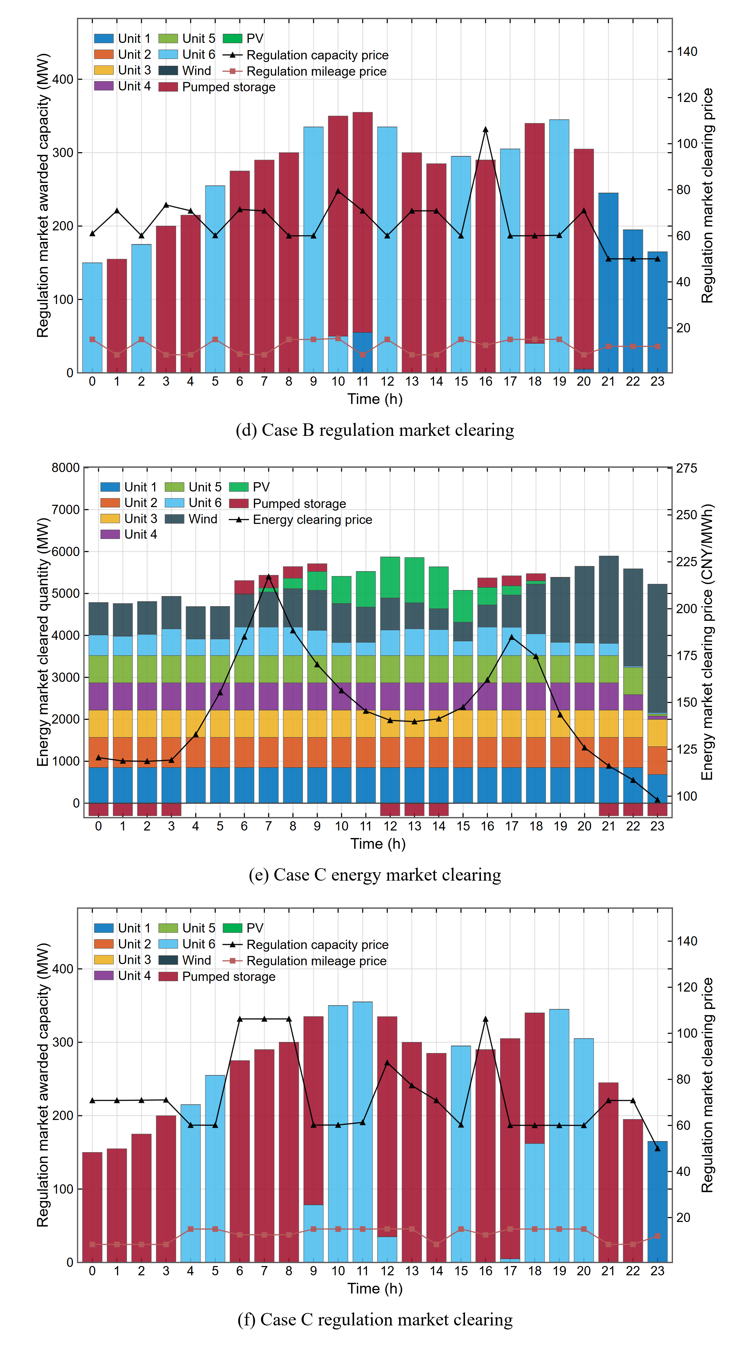
Three cases are defined to quantify the effects of the price and operating state priors. Case A uses only the pumping generation state prior and no forecast price benchmark. Case B uses the forecast price benchmark but no operating state prior. Case C, representing the proposed method, uses both the forecast price benchmark and state selection.
Figure 12a,c,e show the energy market clearing results. In Cases A and C, pumped storage concentrates pumping in low-price periods and generation in the morning and evening high-price periods, broadly matching the price shape of price pattern Scenario 4. In Case B, operating periods are more dispersed and some adjacent periods switch operating modes. Cases A and C use the operating state prior to select modes consistent with the typical pumping generation pattern of the matched scenario, thereby reducing switches that conflict with peak–valley price intervals. Case B relies only on the forecast price and lacks this intra-day operating guidance. The awarded energy quantities also differ between Cases A and C because, once the operating state is fixed, the forecast price benchmark further adjusts period-specific bids.
Figure 12.
Market clearing results under the three bidding cases.
Figure 12b,d,f show the regulation market results. Pumped storage is awarded regulation capacity in more periods under Case C than under Cases A and B. Energy output and regulation capacity share the same physical unit capacity, and a single prior provides only limited coordination between the two markets. By combining the forecast price benchmark with the operating state prior, Case C assesses the economic value of energy participation in each period while identifying capacity available for regulation, enabling coordinated energy and regulation offers.
Table 3 compares revenues across the three cases. Case C does not simply maximize energy market revenue; it allocates capacity across the joint market. Although its generation revenue is lower than those of Cases A and B, assigning part of the available capacity to more profitable regulation service raises net revenue to CNY 730,500, above both alternatives. The forecast price prior provides a day-ahead price benchmark for each period, enabling the plant to compare pumping and generating spreads, estimate the opportunity cost of regulation capacity, and formulate bids that balance revenues from both markets.
Table 3.
Pumped storage revenues under the three bidding cases.
6.2.6. Sensitivity Analysis of the Reference Price Prior
The accuracy of day-ahead price information affects bidding decisions and market outcomes. To examine the sensitivity of the proposed bidding strategy to errors in its reference price prior, Gaussian noise was added to the S4 reference price sequence. The standard deviation of the added noise was set to 10%, 20%, 30%, and 40% of the baseline price forecast residual standard deviation; the unperturbed sequence served as the benchmark. The trained BMARL policy, operating state prior, and market clearing parameters were held fixed. Table 4 reports the resulting changes in pumped storage profit and total market profit.
Table 4.
Sensitivity analysis results of electricity price forecasting error.
As the perturbation increased, mean pumped storage profit declined from CNY 722.09 thousand in the benchmark case to CNY 702.07 thousand at the 40% level, a decrease of 2.77%. Changes at the 10% and 20% levels were small, whereas the decline became more pronounced at the 30% and 40% levels. Mean total market profit also decreased slightly. These exploratory results indicate that the fixed S4 policy tolerates small deviations in the reference price prior, while larger deviations reduce pumped storage profit.
7. Conclusions
This study addresses pumped storage bidding in joint energy regulation markets under incomplete information. A scenario-clustering price forecasting model is developed, and BMARL is used to solve the bidding and joint clearing model. The principal conclusions are as follows.
(1) The proposed forecasting-to-bidding mechanism converts day-ahead price forecasts into pumping, idle, and generating states and a reference price prior, thereby incorporating forecast information directly into bidding decisions. It aligns pumping and generation schedules with peak–valley market price patterns and effectively reduces uneconomic electricity purchases and sales.
(2) This paper proposes an electricity price forecasting model for pumped storage plants that integrates multi-scenario clustering and directed graph structure learning. By partitioning historical electricity price samples into different scenarios, the model reduces the interference of data heterogeneity across diverse price patterns. Within each scenario, it learns directional statistical dependencies and multi-scale temporal features between electricity prices and their influencing factors, improving the capability to capture peak–valley variations of electricity prices on the target day and thereby enhancing the accuracy of day-ahead electricity price forecasting.
(3) The BMARL-based game model effectively characterizes uncertainty in value function estimation caused by incomplete information and changes in competitors’ strategies. In the case study, BMARL reduces the number of training episodes required for convergence by approximately 18.3% relative to the benchmark models and increases pumped storage profit under incomplete information.
It should be noted that several limitations exist in this paper. First, the CatBoost scenario classifier is evaluated primarily on historical operating conditions. Its reliability under ambiguous scenario assignments, rare price patterns, and out-of-distribution exogenous inputs, such as those associated with extreme weather, remains uncertain. Future work should examine how classification errors and low-confidence predictions affect the resulting pumping and generating state priors and bidding outcomes. Second, the present model uses fixed pumping and generating efficiency parameters and does not explicitly account for hydraulic head variation or the wear caused by frequent mode switching. Head-dependent efficiency and switching cost parameters should be incorporated to assess their effects on physical feasibility and bidding profitability. Third, the regulation performance score is treated as fixed. Sensitivity tests with varying and stochastic scores are needed to determine whether the allocation of capacity between the energy and regulation markets remains stable. Fourth, the bidding strategy is evaluated on one test system without systematically varying renewable generation penetration and variability across nodes. Further experiments under multiple renewable penetration levels and output scenarios are required to assess the robustness of BMARL convergence and pumped storage revenue. These extensions will help establish the conditions under which the proposed strategy remains effective.
Author Contributions
Writing—original draft, M.L.; validation, M.L.; methodology, M.L.; software, M.L.; formal analysis, M.L.; Data curation, J.G; conceptualization, J.G; visualization, J.G. All authors have read and agreed to the published version of the manuscript.
Funding
This research received no external funding.
Institutional Review Board Statement
Not applicable.
Informed Consent Statement
Not applicable.
Data Availability Statement
The data presented in this study are available from the corresponding author upon reasonable request.
Conflicts of Interest
The authors declare no conflicts of interest.
Appendix A. BMARL Algorithm Implementation Procedure
The specific steps of the BMARL algorithm are as follows:
- (1)
- Initialize the Actor and Critic networks and their corresponding target networks for each agent. Initialize the experience replay buffer, specify the Gaussian prior distribution of the Bayesian parameters in the final layer of the Critic network, and set the maximum number of training iterations.
- (2)
- Each agent generates a bidding action through its Actor network based on its current local observation and determines the corresponding bidding strategy by incorporating the electricity price forecasting prior and operating state prior.
- (3)
- Input the bidding actions of all agents into the joint market clearing model to obtain the market clearing results. Calculate the reward of each agent based on its net profit and obtain the next state.
- (4)
- Store the current state, bidding action, reward, and next state as a transition in the experience replay buffer.
- (5)
- When the number of samples in the experience replay buffer satisfies the training requirements, randomly sample a batch of experiences from the buffer and perform the following operations:
- ①
- Construct the feature matrix and temporal difference target using the sampled experiences, and update the posterior distribution of the Bayesian parameters in the final layer of the Critic network through Bayesian linear regression.
- ②
- Sample parameters from the posterior distribution to update the current Critic network and construct the target Critic network using the posterior mean.
- ③
- Generate the next-state actions using the target Actor networks and calculate the temporal difference targets by incorporating the maximum entropy regularization term.
- ④
- Update the Critic network by minimizing the value loss function and update the Actor network by minimizing the maximum entropy policy loss function.
- ⑤
- Update the target Actor and Critic networks using the soft update mechanism.
- (6)
- Repeat Steps (2)–(5). Each agent continuously interacts with the joint market environment to update its bidding strategy and Critic network parameters.
- (7)
- Terminate the training when the maximum number of iterations is reached or the convergence criterion is satisfied and output the optimal bidding strategies of all agents.
Appendix B. Electricity Price Forecasting Metrics
Historical data are normalized to remove differences in scale:
where x is the original series, x* is the normalized series, and xmax and xmin are the maximum and minimum values, respectively.
Forecasting performance is evaluated using MAE, RMSE, MAPE, and R2. The metrics are calculated as follows:
where yi and are the actual and forecast prices, respectively, at target day time point i; is the mean day-ahead price over all target day time points; and N is the number of forecast points.
Appendix C. Generator Parameters, Demand, and Renewable Generation Forecasts
Figure A1.
Forecasts of load, wind generation, and photovoltaic generation.
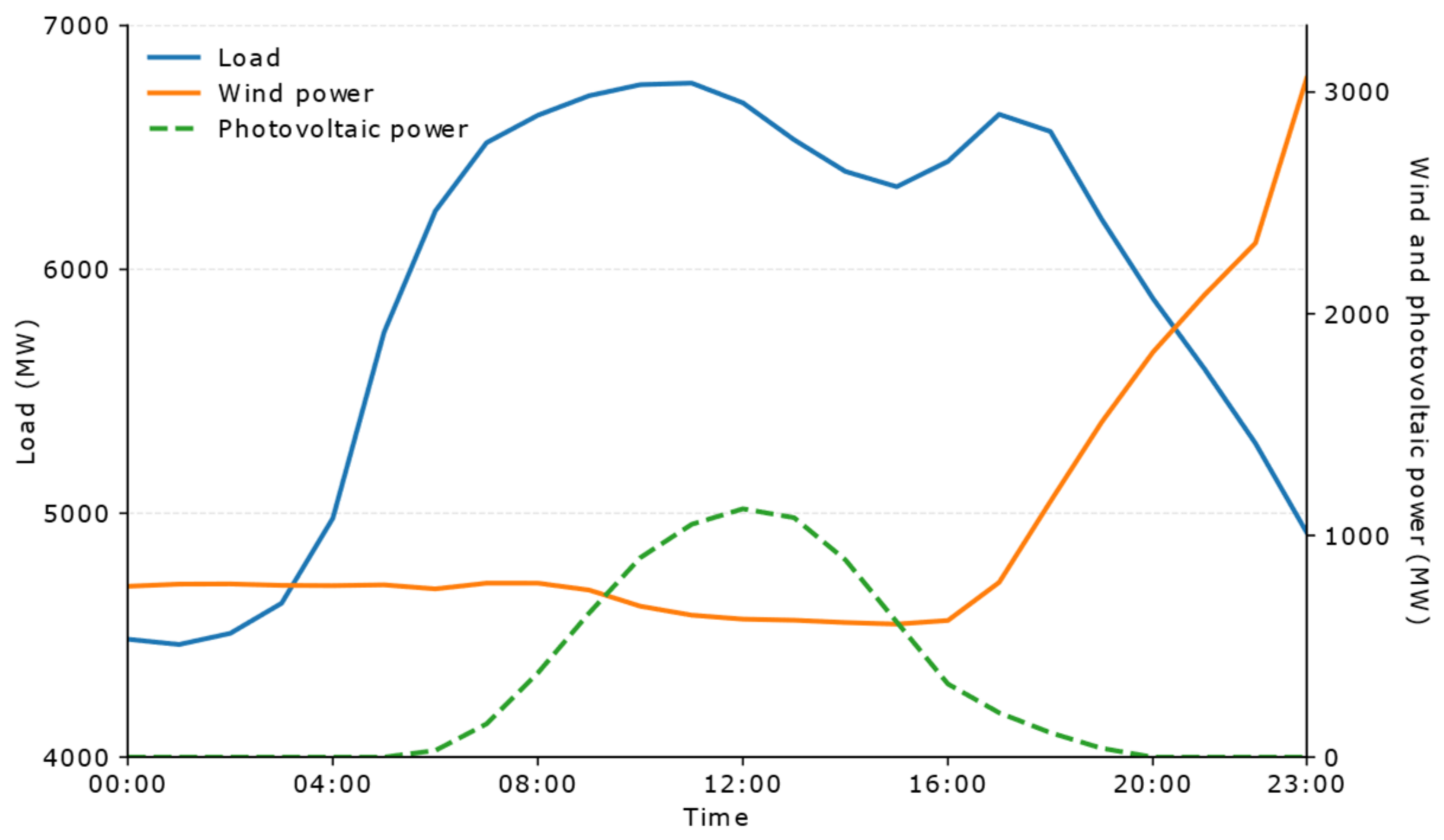
Table A1.
Generator parameters.
Appendix D. Network Architecture and Algorithm Hyperparameters
Table A2.
Network architecture and hyperparameters of the reinforcementlearning methods.
References
- Liu, D.; Yang, Y.; Huang, H.; Zhong, H. An overview and outlook of the operation and control of large-scale pumped hydro storages in modern power systems. Proc. CSEE 2025, 45, 80–98. [Google Scholar] [CrossRef]
- Wen, J.; Zhou, B.; Wei, L. Preliminary study on an energy storage grid for the future power system in China. Power Syst. Prot. Control 2022, 50, 1–10. [Google Scholar] [CrossRef]
- National Development and Reform Commission. Opinions on Further Improving the Price Formation Mechanism for Pumped Storage; NDRC Price [2021] No. 633. 30 April 2021. Available online: https://www.ndrc.gov.cn/xxgk/zcfb/tz/202105/t20210507_1279341.html (accessed on 13 October 2026).
- National Energy Administration. Medium- and Long-Term Development Plan for Pumped Storage (2021–2035). 17 September 2021. Available online: https://zfxxgk.nea.gov.cn/2021-09/17/c_1310193456.htm (accessed on 13 October 2026).
- Ding, H.; Xin, C.; Li, M.; Li, Y.; Zeng, M.; Chen, J.; Zhang, X. Bidding strategies of pumped storage power stations considering electricity spot-market risk. Electr. Power Constr. 2024, 45, 150–158. [Google Scholar] [CrossRef]
- Liu, F.; Che, Y.; Tian, X.; Decao, X.; Huijie, Z.; Zhiyi, L. Optimal operation strategy of pumped-storage hydropower stations considering electricity-market participation risk. Water Resour. Hydropower Eng. 2022, 53, 94–104. [Google Scholar] [CrossRef]
- Liu, J.; Li, L.; Wu, M.; Chen, H.; Chen, H. A two-stage optimal operation strategy for distributed pumped-storage power plants and renewable generation jointly participating in the spot market. Zhejiang Electr. Power 2023, 42, 50–58. [Google Scholar] [CrossRef]
- Lv, W.; Zhao, H.; Han, Y.; Hu, D.; Peng, X. Hierarchical optimal scheduling for pumped storage to enhance system flexibility under supply-demand uncertainty. Trans. China Electrotech. Soc. 2025, 40, 6984–6999. [Google Scholar] [CrossRef]
- Jukic, D.K.; Kugi, A.; Kemmetmuller, W. Optimal operation of pumped-storage power plants with fixed- and variable-speed generators in multiple electricity markets considering overload operation. J. Energy Storage 2024, 88, 111601. [Google Scholar] [CrossRef] [Scilit]
- Pan, L.; Xu, X.; Hu, L.W. Distributionally robust economic scheduling of a hybrid hydro/solar/pumped-storage system considering bilateral-contract flexible decomposition and day-ahead market bidding. J. Clean. Prod. 2023, 428, 139344. [Google Scholar] [CrossRef] [Scilit]
- Huang, L.; Liu, J.; Liu, Y. Capacity allocation strategies for pumped-storage plants that complement renewable energy sources and participate independently in multilevel markets. Power Syst. Technol. 2024, 48, 4948–4957. [Google Scholar]
- Tang, L.; Cai, Y.; Tang, X.; Cao, Y.; Tan, Y. Bi-level optimization strategy considering pumped-storage participation in ancillary services and capacity trading. Power Syst. Technol. 2025, 49, 1469–1478. [Google Scholar]
- Eltamaly, A.M.; Almutairi, Z.A. A novel star-nosed mole optimization algorithm applied for MPPT of PV systems. Sci. Rep. 2025, 15, 17807. [Google Scholar] [CrossRef] [Scilit]
- Liang, Y.; Guo, C.; Ding, Z.; Hua, H. Agent-based modeling in electricity markets using a deep deterministic policy gradient algorithm. IEEE Trans. Power Syst. 2020, 35, 4180–4192. [Google Scholar] [CrossRef] [Scilit]
- Zhao, P.; Wu, J.; Wang, Y.; Zhang, H. Optimal operation strategy of a microgrid based on deep reinforcement learning. Electr. Power Autom. Equip. 2022, 42, 9–16. [Google Scholar] [CrossRef]
- Xu, D.; Hu, X.; Hu, F.; Cha, Y.; Zhang, C.; Yu, Y.; Zhao, Y. Strategic bidding of price-quantity pairs in electricity markets based on deep reinforcement learning. Power Syst. Technol. 2024, 48, 3278–3286. [Google Scholar]
- Du, Y.; Li, F.; Zandi, H.; Xue, Y. Approximating Nash equilibrium in day-ahead electricity-market bidding with multi-agent deep reinforcement learning. J. Mod. Power Syst. Clean Energy 2021, 9, 534–544. [Google Scholar] [CrossRef] [Scilit]
- Yuan, J.; Yang, M.; Liu, N.; Zhang, C.; Huang, S. Bidding strategy of generation companies based on a multi-agent deep deterministic policy-gradient algorithm under incomplete information. Power Syst. Technol. 2022, 46, 4832–4844. [Google Scholar]
- Peng, C.; Yi, T.; Sun, H.; Chen, S. Equilibrium bidding strategies of generators in an electricity-carbon coupled market based on multi-agent deep deterministic policy gradients. Power Syst. Technol. 2023, 47, 4229–4236. [Google Scholar] [CrossRef]
- Schmitt, S.; Shawe-Taylor, J.; Van Hasselt, H. Exploration via Epistemic Value Estimation. Proc. AAAI Conf. Artif. Intell. 2023, 37, 9742–9751. [Google Scholar] [CrossRef] [Scilit]
- Liu, Q.; Li, Y.; Chen, S.; Lin, K.; Shi, X.; Lou, Y. Distributional reinforcement learning with epistemic and aleatoric uncertainty estimation. Inf. Sci. 2023, 644, 16. [Google Scholar] [CrossRef] [Scilit]
- Du, X.; Chen, H.; Wang, C.; Xing, Y.; Yang, J.; Yu, P.S.; Chang, Y.; He, L. Robust multi-agent reinforcement learning via Bayesian distributional value estimation. Pattern Recognit. 2024, 145, 11. [Google Scholar] [CrossRef] [Scilit]
- Jan, F.; Iftikhar, H.; Tahir, M.; Khan, M. Forecasting day-ahead electric-power prices with functional data analysis. Front. Energy Res. 2025, 13, 1477248. [Google Scholar] [CrossRef] [Scilit]
- Gu, K.; Jia, L. Temporal convolutional network-based short-term load forecasting model. In Proceedings of the 2020 Chinese Control and Decision Conference; IEEE: New York, NY, USA, 2020. [Google Scholar] [CrossRef] [Scilit]
- Ji, X.; Zeng, R.; Zhang, Y.; Song, F.; Sun, P.; Zhao, G. CNN-LSTM short-term electricity-price forecasting based on an attention mechanism. Power Syst. Prot. Control 2022, 50, 125–132. [Google Scholar] [CrossRef]
- Nafea, A.A.; Alawi, O.A.; Doost, Z.H.; AlAni, M.; Ahmadullah, A.B.; Deo, R.C.; Yaseen, Z.M. Electricity load and price forecasting in Spain: A hybrid deep-learning framework leveraging temporal and seasonal dynamics. Expert Syst. Appl. 2026, 299, 130123. [Google Scholar] [CrossRef] [Scilit]
- Meng, A.; Zhu, J.; Yan, B.; Yin, H. Day-ahead electricity-price prediction in multiple price zones based on a multi-view fusion spatiotemporal graph neural network. Appl. Energy 2024, 369, 123553. [Google Scholar] [CrossRef] [Scilit]
- Yang, Y.; Guo, J.; Li, Y.; Zhou, J. Forecasting day-ahead electricity prices with spatial dependence. Int. J. Forecast. 2024, 40, 1255–1270. [Google Scholar] [CrossRef] [Scilit]
- Jung, B.W.; Lee, D.S.; Son, S.Y. Distribution-system nodal-voltage forecasting based on GCN-LSTM. IEEE Access 2026, 14, 50270–50281. [Google Scholar]
- Wu, Z.; Pan, S.; Long, G.; Jiang, J.; Chang, X.; Zhang, C. Connecting the Dots: Multivariate Time Series Forecasting with Graph Neural Networks. In Proceedings of the 26th ACM SIGKDD International Conference on Knowledge Discovery and Data Mining; ACM: New York, NY, USA, 2020. [Google Scholar] [CrossRef] [Scilit]

Disclaimer/Publisher’s Note: The statements, opinions and data contained in all publications are solely those of the individual author(s) and contributor(s) and not of MDPI and/or the editor(s). MDPI and/or the editor(s) disclaim responsibility for any injury to people or property resulting from any ideas, methods, instructions or products referred to in the content. |
© 2026 by the authors. Licensee MDPI, Basel, Switzerland. This article is an open access article distributed under the terms and conditions of the Creative Commons Attribution (CC BY) license.