Short-Term Electricity Load Forecasting via CNN-KAN Heterogeneous Feature Mapping with Recursive Smoothing Soft B-Spline Basis Enhancement

Abstract

Electricity load forecasting is essential for the optimal operation of smart grids and effective energy scheduling. However, increasing uncertainties caused by complex power system operations, renewable energy integration, and changes in user behavior have made load series more nonstationary and nonlinear. Traditional forecasting methods and existing deep learning models still have limitations in modeling such complex nonlinear relationships. To improve the nonlinear representation capability of short-term load forecasting models, this paper proposes a CNN-KAN framework based on heterogeneous feature mapping. The proposed method first employs a convolutional neural network to extract local temporal dependency features from multivariate historical load sequences. A Kolmogorov–Arnold Network is then used to perform adaptive nonlinear function mapping. In addition, a recursive smoothing soft B-spline basis mapping mechanism is introduced to improve the continuity and adaptability of the basis representation in KAN. Experiments are conducted on the Tetouan City electricity load dataset under two forecasting scenarios, namely Quads and Combined. The model is evaluated using MSE, RMSE, MAE, $R^2$, and MAPE. Experimental results show that CNN-KAN achieves stable forecasting performance in both scenarios. The $R^2$ values exceed 0.99, while the MAPE values remain below 1%. The proposed model demonstrates competitive overall forecasting performance compared with the Decision Tree, LSTM, TCN, and Informer baselines across the two forecasting scenarios. These results demonstrate the effectiveness of the proposed CNN-KAN heterogeneous feature mapping framework for short-term electricity load forecasting.

1. Introduction

Electricity load forecasting is essential for the optimal operation of smart grids, energy scheduling, and electricity market decision making. With the large-scale integration of renewable energy, changes in user electricity consumption behavior, and increasing complexity of power system operations, electricity load series have become increasingly nonstationary, stochastic, and nonlinear. These characteristics pose greater challenges to short-term load forecasting. Accurate prediction of short-term load variations can improve power system operation and support generation planning, demand response management, and optimal energy resource allocation [1,2,3,4].

Recent studies have further highlighted the practical and economic implications of load forecasting errors. In a study of a real residential building, the daily mean absolute percentage error was approximately 12%, and the peak power cost increased by 20.2% compared with the ideal case of perfect forecasting, although no significant differences in total operating costs were observed among the tested scheduling cases [5]. Similarly, Rabie et al. investigated the financial implications of load forecasting errors in the Japanese electricity market under different regional demand and market price conditions, demonstrating that the economic consequences varied considerably across operating scenarios [6]. These findings indicate that forecasting errors can affect specific operating costs and that their financial implications depend on the characteristics of the power system and electricity market.

Therefore, effectively modeling the complex relationships between historical load data and external environmental factors has become an important research topic in intelligent power systems. In particular, forecasting models require sufficient nonlinear representation capability to capture complex load variations.

Early studies on electricity load forecasting mainly relied on statistical methods [7], such as the autoregressive moving average (ARMA) model [8] and the autoregressive integrated moving average (ARIMA) model [9]. These methods have simple structures and good interpretability. They can provide satisfactory forecasting results for relatively stable load series. However, they usually rely on predefined statistical assumptions and linear relationships. Their forecasting capability may therefore be limited when dealing with nonlinear variations, interactions among multiple influencing factors, and complex dynamic patterns in practical power systems. Machine learning methods were subsequently introduced into electricity load forecasting. These methods learn the mapping between input variables and load variations in a data-driven manner. Representative approaches include artificial neural networks (ANNs) [10] and support vector machines (SVMs) [11], which have improved forecasting performance to some extent. However, these methods generally rely on manually designed features. Their capability to automatically extract useful representations from high-dimensional, multivariate, and complex time-series data remains limited. As a result, they may not fully capture the complex nonlinear relationships underlying electricity load variations.

With the development of deep learning, neural network-based data-driven methods have become an important research direction for electricity load forecasting [12]. Compared with traditional methods, deep learning models can automatically learn latent feature representations through multilayer network structures. This reduces their dependence on manual feature engineering and provides stronger modeling capability for complex time-series forecasting tasks. Convolutional neural networks (CNNs) can capture local temporal patterns in multivariate load sequences through local receptive fields and parameter sharing. They have therefore been widely applied to short-term electricity load forecasting [13]. Recurrent neural networks (RNNs) [14] and their variant, long short-term memory (LSTM) networks [15], use recurrent structures to model temporal dependencies. They have shown good performance in load sequences with long-term dependencies. Attention-based Transformer models have also been used to capture global dependencies in complex time series. However, existing deep learning models commonly employ predefined activation functions for nonlinear transformations. Such feature transformations have limited adaptability. There is still room to improve their capability to represent complex nonlinear relationships and dynamic variations in electricity load data.

In recent years, the Kolmogorov–Arnold Network (KAN) has emerged as a new neural network architecture for modeling complex nonlinear relationships [16]. Unlike conventional neural networks that combine learnable weights with fixed activation functions, KAN employs learnable univariate function mappings instead of fixed activation functions in conventional neurons. This design provides greater flexibility for approximating complex nonlinear functional relationships. Its spline-based parameterization further enhances the capability to model continuous functional relationships. KAN has therefore shown promising potential for scientific computing and complex prediction tasks. However, directly applying the original KAN to short-term electricity load forecasting still presents challenges [17]. Electricity load series exhibit local fluctuations and dynamic variations. Effective extraction of local relationships between historical loads and external factors is therefore necessary. In addition, the basis representation of the original KAN relies on predefined spline basis partitions. Its local continuity and feature adaptability may affect the modeling of complex time-series data. Therefore, further research is needed to combine deep temporal feature extraction with an enhanced nonlinear function representation mechanism for short-term electricity load forecasting.

To address these issues, this paper proposes a short-term electricity load forecasting method based on CNN-KAN heterogeneous feature mapping. A recursive smoothing soft B-spline basis mapping mechanism is introduced into the KAN module to enhance the representation of complex nonlinear load variations. The proposed method first employs a CNN to extract local temporal dependency features from multivariate historical load sequences. The enhanced KAN module then performs adaptive nonlinear feature mapping. In this way, the framework integrates local pattern extraction with nonlinear feature reconstruction. The main contributions of this work are summarized as follows:

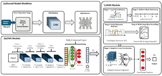
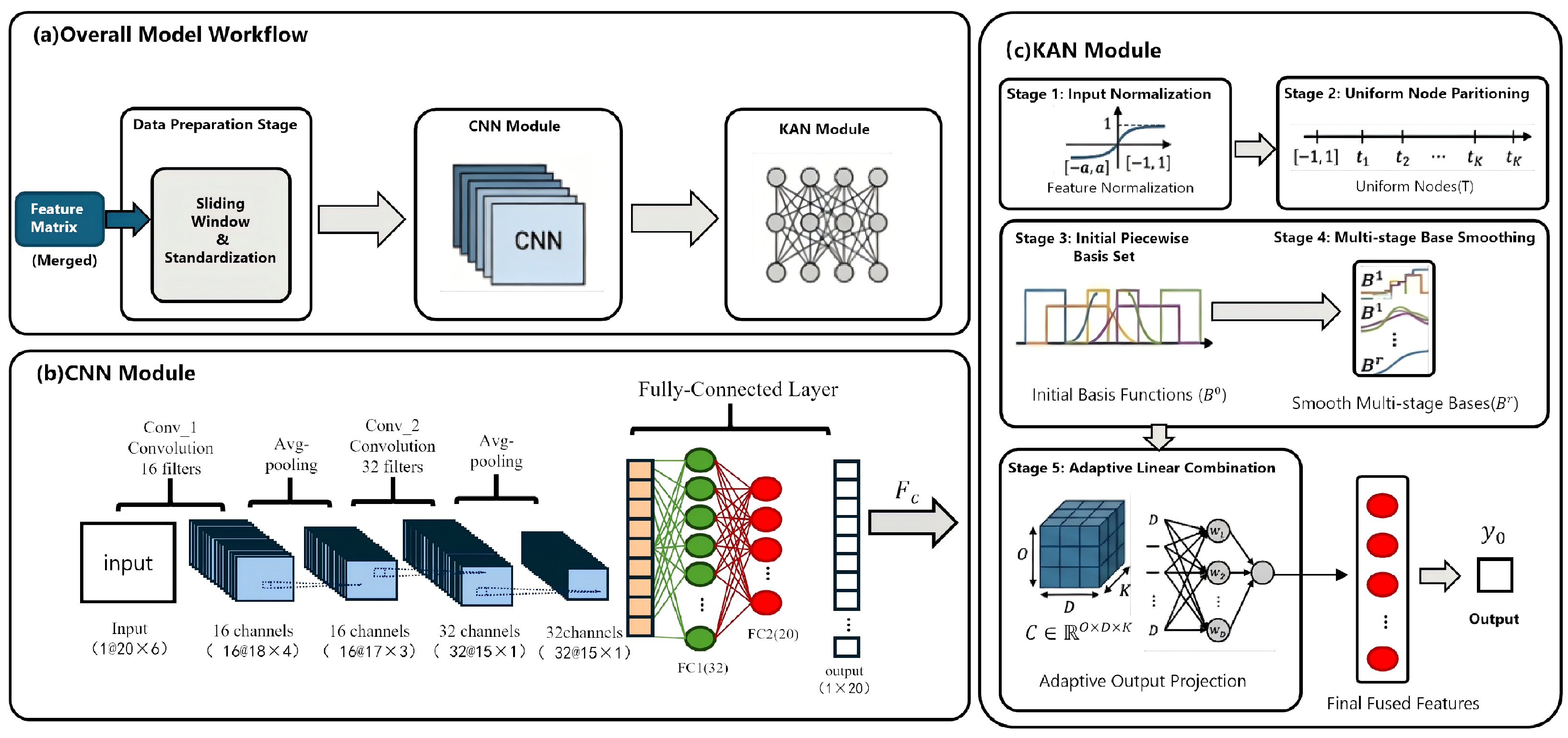
• A CNN-KAN heterogeneous feature mapping framework is proposed, as illustrated in Figure 1. It integrates the local temporal feature extraction capability of CNN with the learnable nonlinear function representation capability of KAN. This framework enables joint modeling of complex short-term electricity load variation patterns.
  

  Figure 1. CNN-KAN heterogeneous feature mapping framework.
• A recursive smoothing soft B-spline basis mapping mechanism is proposed. It constructs continuous soft interval responses and applies a recursive neighborhood smoothing strategy. This mechanism improves the continuity and feature adaptability of the KAN basis representation, thereby enhancing the representation of complex nonlinear load relationships.
• Two forecasting scenarios, Quads and Combined, are constructed using the Tetouan City electricity load data. The effectiveness of the proposed method is evaluated using multiple performance metrics, comparisons with baseline models, and parameter sensitivity analysis.

2. Related Works

2.1. Traditional and Machine Learning-Based Load Forecasting Methods

Early studies on short-term electricity load forecasting mainly relied on statistical models, such as autoregressive moving average (ARMA) [8] and autoregressive integrated moving average (ARIMA) [9], which estimate future load values based on historical patterns and statistical assumptions. These methods have advantages in terms of simplicity and interpretability, and they have achieved satisfactory performance for relatively stable load series. However, due to their reliance on predefined assumptions and limited nonlinear representation capability, statistical models may struggle to capture complex load variations caused by multiple influencing factors, such as weather conditions, user behaviors, and system dynamics.

To overcome the limitations of statistical approaches, machine learning methods have been increasingly applied to electricity load forecasting. Models such as artificial neural networks (ANNs) [10], support vector machines (SVMs) [11], and ensemble learning methods [18,19,20] learn nonlinear relationships between input variables and load values in a data-driven manner, thereby improving prediction performance compared with traditional statistical approaches. Nevertheless, these methods generally depend on manually designed features and have limited capability in automatically extracting hierarchical representations from high-dimensional multivariate time-series data. Therefore, further research has focused on deep learning-based forecasting approaches, which can automatically learn complex temporal patterns from raw data.

2.2. Deep Learning-Based Load Forecasting Methods

With the rapid development of deep learning, neural network-based methods have become widely used in short-term electricity load forecasting due to their powerful feature learning capability. Compared with traditional machine learning methods, deep learning models can automatically extract hierarchical representations from raw load sequences and effectively model complex nonlinear relationships between input variables and electricity demand.

Convolutional neural networks (CNNs) have been introduced into load forecasting tasks due to their ability to capture local temporal patterns through convolution operations. By constructing multiple convolutional layers, CNN-based models can extract short-term fluctuation characteristics and correlations among multivariate load-related variables, thereby improving forecasting performance. Several studies have demonstrated the effectiveness of CNN-based architectures in short-term load forecasting tasks [21,22].

Recurrent neural networks (RNNs) and their variants, especially long short-term memory networks (LSTMs), have also been extensively investigated for load forecasting because of their capability to model temporal dependencies. LSTM-based approaches can alleviate the gradient vanishing problem of conventional RNNs and capture long-range dependencies in load sequences [23]. Furthermore, hybrid CNN-LSTM models have been developed by combining CNN-based feature extraction with LSTM-based temporal modeling, achieving improved performance by jointly exploiting local patterns and sequential dependencies [24].

Despite the effectiveness of existing deep learning models, most approaches still rely on predefined activation functions to perform nonlinear transformations. Such fixed nonlinear mappings may limit the adaptability of models when dealing with highly complex load variations and dynamic interactions among multiple influencing factors. Therefore, more flexible nonlinear representation mechanisms are required to further enhance the modeling capability of short-term electricity load forecasting models.

2.3. Kolmogorov–Arnold Networks and Nonlinear Representation Learning

Recently, Kolmogorov–Arnold Networks (KANs) have attracted increasing attention as an alternative neural network architecture for nonlinear representation learning. Inspired by the Kolmogorov–Arnold representation theorem, KAN replaces fixed activation functions in conventional neural networks with learnable univariate function mappings on network edges, providing a more flexible mechanism for modeling complex nonlinear relationships. In the original KAN framework, spline functions are employed to parameterize learnable functions, enabling adaptive nonlinear approximation and improving model interpretability compared with traditional multilayer perceptron architectures [16].

Due to these advantages, KAN-based methods have been explored in various scientific and engineering applications, including function approximation, scientific machine learning, and physics-informed modeling [25,26]. These studies demonstrate the potential of learnable function representations for capturing complex nonlinear relationships. However, most existing KAN-related studies mainly focus on low-dimensional regression or scientific computing problems, while their applications to multivariate time-series forecasting tasks remain relatively limited.

For short-term electricity load forecasting, directly applying the original KAN architecture may not fully exploit the local temporal patterns contained in historical load sequences. Moreover, the spline-based function representation used in KAN requires effective basis construction to maintain smooth nonlinear transformations when dealing with complex dynamic data. Therefore, integrating KAN with dedicated temporal feature extraction mechanisms and enhancing the adaptability of spline-based representations are important directions for improving KAN-based forecasting models.

3. Method

3.1. Data Preprocessing and Sliding Window Construction

To capture the temporal dependencies in electricity load data and construct samples for model training, a sliding window strategy is applied to the original time series. The sliding window process is illustrated in the left part of Figure 1a. The original multivariate electricity load sequence is represented as

$$X=\{x_1,x_2,\dots ,x_t,\dots ,x_T\},x_t\in {\mathbb{R}}^F$$

(1)

where $x_t$ denotes the electricity load and its associated features at time step t, and F denotes the number of input features.

For the original time series, a sliding window with length L and step size s is used to construct input samples. The i-th sample after window reconstruction is expressed as

$$X_i=[x_i,x_{i+1},\cdots ,x_{i+L-1}]$$

(2)

The corresponding forecasting target is defined as

$$Y_i=y_{i+L}$$

(3)

Here, $X_i\in {\mathbb{R}}^{L\times F}$ represents the multivariate historical feature sequence containing L consecutive time steps. F denotes the feature set associated with multiple types of information, including historical electricity load, temperature, humidity, wind speed, and other influencing factors. $Y_i$ is the electricity load at the next time step after the end of the input window and serves as the target value to be predicted.

The sliding window moves along the time axis with a step size of s. In this way, the original time-series data are transformed into a supervised learning dataset:

$$\mathcal{D}={\left\{(X_i,Y_i)\right\}}_{i=1}^N$$

(4)

It should be noted that the meteorological variables included in the input features are used to capture their statistical associations with electricity load variations for predictive purposes. Although factors such as temperature, humidity, and wind speed may be associated with changes in electricity demand, the relationships learned by the proposed model do not necessarily represent causal effects. Electricity load is also influenced by other factors, including time-dependent consumption patterns, human activities, and operational conditions. Therefore, this study focuses on short-term electricity load forecasting based on historical observations rather than causal inference. In the context of climate change, changes in meteorological conditions may alter electricity consumption patterns and affect the generalizability of forecasting models. However, assessing the causal impacts of climate change on electricity demand is beyond the scope of this study.

3.2. Multivariate Load Feature Extraction with CNN

The proposed model employs a 2D CNN to extract local patterns from multivariate electricity load data. The architecture of the CNN module is illustrated in Figure 1b. The input data are represented as a single-channel tensor and processed by two convolution-pooling units. The first convolutional layer scans the input sequence using a set of convolution kernels to extract local patterns from the original data. The second convolutional layer increases the number of channels to obtain higher-level feature representations. No padding is used in either convolutional layer. This setting avoids introducing artificial values at the boundaries and ensures that convolution operations are performed only on the original input data.

A hierarchical pooling strategy is adopted to balance feature preservation and computational efficiency. Average pooling is used after the first convolutional layer with a predefined kernel size and a relatively small stride. This operation smooths local variations during downsampling while retaining useful information from the load sequence. A smaller pooling kernel is used in the second pooling stage to further adjust the feature representation while limiting excessive dimensionality reduction.

The resulting multidimensional feature maps are then flattened into a one-dimensional feature vector and processed by two fully connected layers to obtain higher-level representations. An activation function is applied to each fully connected layer to enhance nonlinear representation capability. Specifically, LeakyReLU is used to facilitate gradient propagation. Unlike ReLU, LeakyReLU retains a small nonzero slope for negative inputs. This property allows gradients to propagate through the negative region and reduces the risk of inactive neurons. The LeakyReLU function is defined as

$$\mathrm{LeakyReLU}\left(x\right)=\left\{\begin{array}{cc}x,\hfill & x\ge 0\hfill \\ 0.01x,\hfill & x<0\hfill \end{array}\right.$$

(5)

To improve the flexibility of the network architecture, the input dimension of the fully connected layer is determined dynamically according to the size of the feature maps produced by the convolution and pooling operations. This avoids manually redefining the fully connected layer when the sliding window length or the number of input features changes. The output dimensions are calculated as follows:

$$\begin{array}{cc}\hfill H_{out}& =(W-K_1+1)-P_1+1-K_2+1\hfill \\ \hfill W_{out}& =(F-K_1+1)-P_1+1-K_2+1\hfill \end{array}$$

(6)

Here, $H_{out}$ and $W_{out}$ denote the height and width of the final CNN feature maps, respectively. W denotes the sliding window length, and F is the number of features at each time step. $K_1$ and $K_2$ denote the kernel sizes of the first and second convolutional layers, respectively. $P_1$ denotes the kernel size of the first pooling operation used for downsampling.

During forward propagation, the input samples are first expanded along the channel dimension. Convolution, pooling, and activation operations are then applied sequentially to extract local representations from the multivariate load data. The resulting feature maps are flattened to obtain a feature representation suitable for the subsequent KAN module. The CNN output is expressed as

$$F_c=[f_1,f_2,\cdots ,f_D]$$

(7)

where D denotes the dimension of the feature vector generated by the CNN module.

3.3. KAN Nonlinear Enhancement via Recursive Smoothing Soft B-Spline Basis Mapping

For short-term electricity load forecasting, CNNs can capture local dependency patterns across consecutive time steps and multiple influencing factors through local receptive fields. However, their feature transformations mainly rely on predefined activation functions. This may limit their ability to represent complex and nonstationary nonlinear relationships in load variations. To further enhance the modeling capability for complex load patterns, a KAN module is introduced after the CNN feature extraction module. Based on the concept of local B-spline basis representation, a recursive smoothing soft B-spline basis mapping mechanism is developed. This mechanism first constructs local basis responses using continuously differentiable soft interval functions. Recursive neighborhood smoothing is then applied to establish relationships between adjacent basis functions. Finally, learnable coefficients are used to perform adaptive nonlinear mapping from the basis function space to the output space.

As illustrated in Figure 1c, the proposed module consists of five stages: feature normalization, uniform knot construction, soft spline basis expansion, recursive neighborhood smoothing, and adaptive output mapping. Instead of using discrete interval indicator functions, the proposed method constructs soft interval responses with continuous transitions using sigmoid functions. This allows the basis representation to vary smoothly near adjacent knot regions. The responses of neighboring basis functions are then progressively integrated through recursive smoothing. This process strengthens the interactions between adjacent local regions. It should be noted that this recursive procedure is not the standard order recursion of B-splines. Instead, it is a neighborhood smoothing strategy specifically designed for KAN feature mapping. Its purpose is to reduce abrupt changes near basis boundaries while preserving local response characteristics.

First, the feature vector $F_c$ generated by the CNN module is normalized using the hyperbolic tangent function:

$$\widehat{f_d}=\tanh \left(f_d\right),d=1,2,\dots ,D$$

(8)

This operation maps the CNN output features to the interval $[-1,1]$, which is consistent with the domain of the spline knots defined in the subsequent stage.

Next, K uniformly spaced knots are constructed in the normalized feature space:

$$T=\{t_1,t_2,\cdots ,t_K\},-1=t_1<\cdots <t_K=1$$

(9)

To avoid abrupt changes at knot boundaries caused by conventional zero-order interval indicator functions, a sigmoid-based soft B-spline basis response is constructed for the i-th knot interval:

$$B_i^{\left(0\right)}\left(x\right)=\sigma \left({\displaystyle \frac{\alpha (x-t_i)}{t_{i+1}-t_i+\epsilon }}\right)\sigma \left({\displaystyle \frac{\alpha (t_{i+1}-x)}{t_{i+1}-t_i+\epsilon }}\right)$$

Here, $\sigma (·)$ denotes the sigmoid function, $\alpha$ controls the steepness of the transition near the interval boundaries, and $\epsilon$ is a small positive constant introduced to prevent division by zero during interval normalization. Both parameters are predefined constants rather than learnable parameters. They are specified before training and remain fixed throughout the experiments. Compared with a hard interval indicator function, the proposed soft basis function provides a continuous response near knot boundaries, thereby yielding a smoother local feature representation for subsequent nonlinear mapping.

For an input feature ${\widehat{f}}_d$, its initial soft spline basis representation is expressed as

$$B^{\left(0\right)}\left(\widehat{f_d}\right)=[B_1^{\left(0\right)}\left(\widehat{f_d}\right),B_2^{\left(0\right)}\left(\widehat{f_d}\right),\cdots ,B_K^{\left(0\right)}\left(\widehat{f_d}\right)]$$

(10)

After obtaining the initial local basis responses, a recursive neighborhood smoothing strategy is applied to strengthen the relationships between adjacent knot regions. The r-th smoothing operation is defined as

$$B_i^{\left(r\right)}\left(x\right)={\displaystyle \frac{B_i^{(r-1)}\left(x\right)+B_{i+1}^{(r-1)}\left(x\right)}{2}},r=1,\cdots ,R.$$

(11)

Here, R denotes the number of recursive smoothing operations. At each recursion step, the local responses of two adjacent basis functions are averaged. This operation progressively establishes neighborhood relationships among initially localized basis regions. After multiple recursive smoothing operations, the resulting basis functions retain their responses to local input regions while providing smoother transitions between adjacent knots. This representation provides a flexible basis for modeling complex nonlinear load variations.

After recursive smoothing, let $K^{\prime }$ denote the number of effective basis functions. A learnable coefficient tensor is introduced to perform adaptive mapping from the basis function space to the output space:

$$C\in R^{O\times D\times K^{\prime }}$$

(12)

Here, D and O denote the input and output feature dimensions, respectively, and $K^{\prime }$ denotes the number of effective basis functions after recursive smoothing. For the o output feature, the mapping is expressed as

$$y_o={\displaystyle \sum _{d=1}^D}{\displaystyle \sum _{k=1}^{K^{\prime }}}{c}_{odk}{B}_k\left({\widehat{f}}_d\right)+b_o$$

(13)

Here, $c_{odk}$ denotes the learnable coefficient associated with the k-th basis function of the d-th input feature for the o output feature, and $b_o$ denotes the corresponding bias term. During end-to-end training, the coefficients and biases are optimized according to the load forecasting objective. Thus, the KAN module maps the CNN feature representation to the target load space through a learnable nonlinear transformation.

3.4. Loss Function

After feature extraction and nonlinear mapping, the output of the model is used to obtain the final electricity load prediction. The predicted value is expressed as

$$\widehat{y_i}=f(X_i;\mathsf{\Theta })$$

(14)

where $X_i$ denotes the input feature sequence, $f(·;\mathsf{\Theta }))$ represents the proposed CNN-KAN forecasting model with model parameters $\mathsf{\Theta }$, and $\widehat{y_i}$ denotes the predicted electricity load.

To optimize the model parameters, MSE is adopted as the loss function:

$${\mathcal{L}}_{\mathrm{MSE}}={\displaystyle \frac{1}{N}}{\displaystyle \sum _{i=1}^N}{(y_i-{\widehat{y}}_i)}^2$$

(15)

where N denotes the number of training samples, $y_i$ is the actual electricity load of the i-th sample, and ${\widehat{y}}_i$ is the corresponding predicted value.

4. Results

4.1. Experimental Settings and Evaluation Metrics

All experiments were conducted on a computer running Ubuntu 24.04 with Python 3.9. PyTorch 2.4.1 and torchvision 0.19.1 were used for model implementation and training, with CUDA 12.1 enabled for GPU acceleration. The hardware platform was equipped with an NVIDIA GeForce RTX 3090 GPU.

To ensure the reliability of the experimental evaluation, all samples are divided in chronological order without random splitting. The first 90% of the samples are used as the development set, while the remaining 10% are used as the test set. The development set is further divided chronologically, with 90% used for training and 10% used for validation. This strategy preserves the temporal order of the load data and prevents future information from entering the model training process.

Before model training, the input features and target load values are standardized. The mean and standard deviation are calculated using only the training set. The same statistical parameters are then applied to the validation and test sets. This ensures that information from the validation and test sets is not introduced during data preprocessing.

The model is trained using the Adam optimizer. The maximum number of training epochs is set to 400. During training, the model performance is evaluated on the validation set after each epoch, and the model parameters corresponding to the lowest validation loss are saved. An early stopping strategy with a patience of 50 epochs is adopted. If the validation loss does not improve for 50 consecutive epochs, the training process is terminated. After training, the model parameters corresponding to the best validation performance are reloaded and used for the final evaluation on the test set.

To comprehensively evaluate the forecasting performance of the proposed model, five commonly used regression metrics are adopted: mean squared error (MSE), root mean squared error (RMSE), mean absolute error (MAE), coefficient of determination ($R^2$), and mean absolute percentage error (MAPE). These metrics evaluate prediction errors from different perspectives and are defined as follows:

$$\begin{array}{cc}\hfill \mathrm{MSE}=& {\displaystyle \frac{1}{n}}{\displaystyle \sum _{i=1}^n}{(y_i-{\widehat{y}}_i)}^2\hfill \end{array}$$

(16)

$$\begin{array}{cc}\hfill \mathrm{RMSE}=& \sqrt{{\displaystyle \frac{1}{N}}\sum _{i=1}^N{(y_i-{\widehat{y}}_i)}^2}\hfill \end{array}$$

(17)

$$\begin{array}{cc}\hfill \mathrm{MAE}=& {\displaystyle \frac{1}{N}}{\displaystyle \sum _{i=1}^N}|y_i-{\widehat{y}}_i|\hfill \end{array}$$

(18)

$$\begin{array}{cc}\hfill R^2=& 1-{\displaystyle \frac{{\sum }_{i=1}^n{(y_i-{\widehat{y}}_i)}^2}{{\sum }_{i=1}^n{(y_i-\overline{y})}^2}}\hfill \end{array}$$

(19)

$$\begin{array}{cc}\hfill \mathrm{MAPE}=& {\displaystyle \frac{100\%}{N}}{\displaystyle \sum _{i=1}^N}\left|{\displaystyle \frac{y_i-{\widehat{y}}_i}{y_i}}\right|\hfill \end{array}$$

(20)

where N denotes the number of samples, $y_i$ is the actual electricity load of the i-th sample, ${\widehat{y}}_i$ is the corresponding predicted value, and $\overline{y}$ denotes the mean of the actual load values. Lower values of MSE, RMSE, MAE, and MAPE indicate smaller forecasting errors, while an $R^2$ value closer to 1 indicates a better fit between the predicted and actual values.

4.2. Dataset and Forecasting Scenarios

The experiments are conducted using the publicly available Tetouan City electricity load dataset [27]. The dataset contains electricity consumption and meteorological data collected in Tetouan City from 1 January to 30 December 2017, at 10-min intervals, with a total of 52,417 observations. The meteorological variables include Temperature, Humidity, Wind Speed, General Diffuse Flows, and Diffuse Flows. In addition, the dataset provides electricity load data for three different zones.

To evaluate the forecasting performance of the proposed model under different load aggregation scales, two forecasting scenarios, namely Quads and Combined, are constructed. In the Quads scenario, the electricity load of a single region is used as the forecasting target. In the Combined scenario, the electricity loads of the three regions are aggregated to construct the target load series. These two scenarios represent different load aggregation scales and are used to evaluate the adaptability of the proposed model under different load characteristics.

For both forecasting scenarios, the model input consists of the historical target load and five environmental variables: Temperature, Humidity, Wind Speed, General Diffuse Flows, and Diffuse Flows. Therefore, each time step contains six input features. After sliding window construction, the input sample can be represented as

$$X_i\in {\mathbb{R}}^{L\times 6}$$

(21)

where L denotes the sliding window length. This input representation enables the model to jointly capture local temporal patterns in historical load data and their relationships with multiple environmental factors.

4.3. Prediction Performance of CNN-KAN

To evaluate the forecasting performance of CNN-KAN, experiments are conducted under the Quads and Combined scenarios. The model performance is analyzed from multiple perspectives, including training and validation loss, evaluation metrics during training, predicted and actual load values, and prediction error metrics.

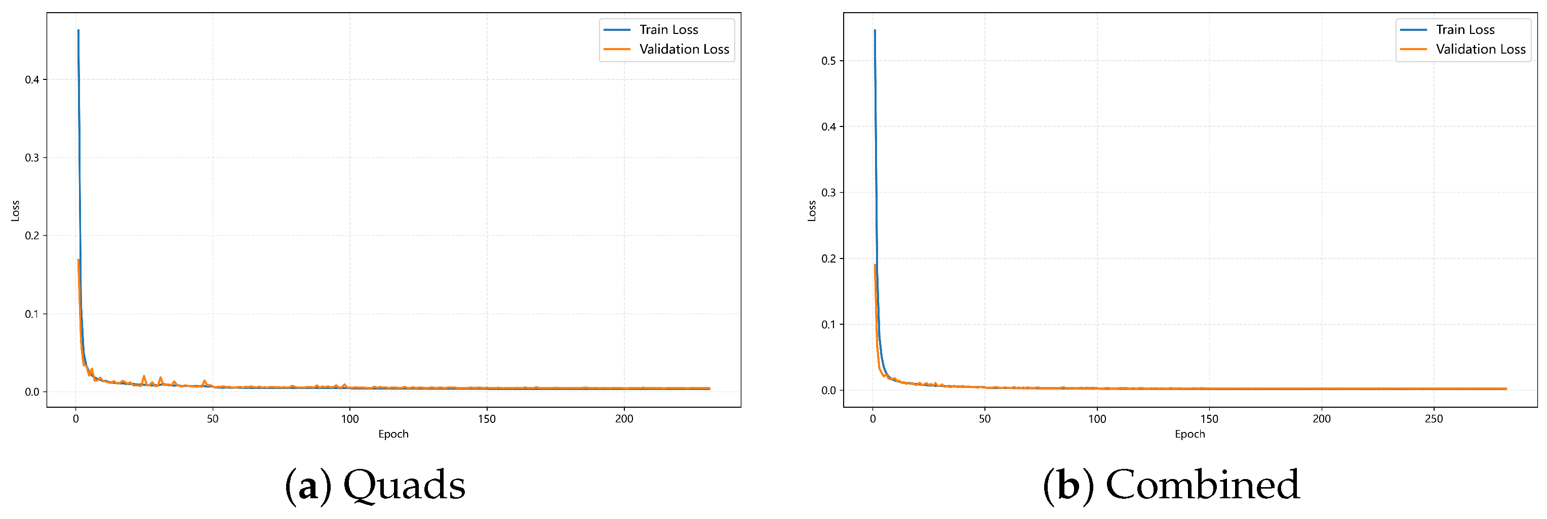
Figure 2 shows the changes in training and validation loss during model training. In both forecasting scenarios, the loss decreases rapidly during the early training stage and then gradually stabilizes as the number of epochs increases. The training and validation loss curves exhibit similar trends, with no obvious separation between them. These results indicate that the optimization process is stable under the current experimental settings.

Figure 2. Training and validation loss of CNN-KAN.

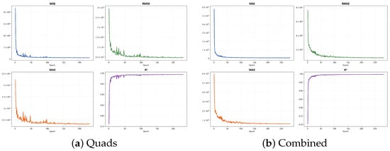
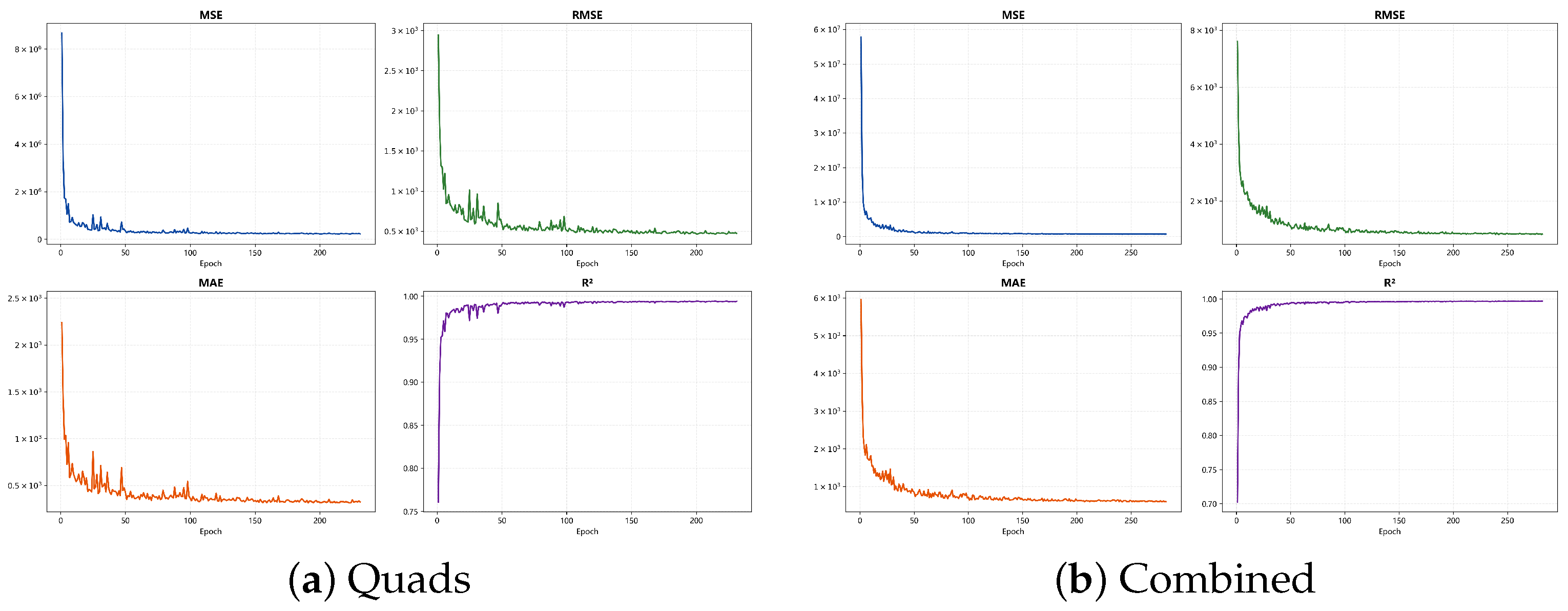
Figure 3 shows the changes in the evaluation metrics calculated on the validation set during training. As training progresses, MSE, RMSE, MAE, and MAPE gradually decrease and then stabilize, while $R^2$ gradually increases and approaches a stable level. Similar trends are observed in both the Quads and Combined scenarios. The evolution of these metrics is consistent with the loss curves in Figure 2, indicating that the model gradually converges during training.

Figure 3. Changes in validation metrics during CNN-KAN training.

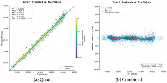
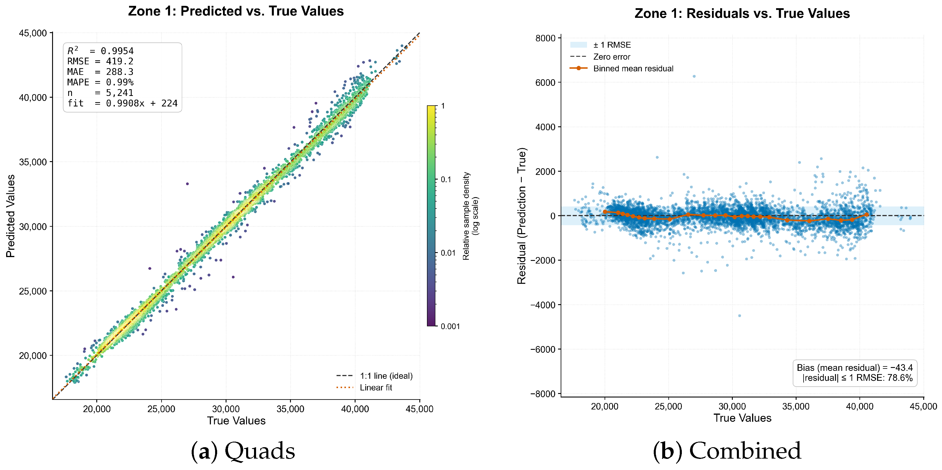
Figure 4 presents the scatter distribution of predicted versus actual electricity loads and the corresponding residuals for Zone 1. In the left panel, the scatter points are closely concentrated around the 1:1 reference line. The linear regression equation is $\widehat{y}=0.9908x+224$, with an $R^2$ of 0.9954, an RMSE of 419.2, an MAE of 288.3, and a MAPE of 0.99% across 5241 test samples. The regression slope is close to 1, and the intercept is relatively small, indicating good agreement between predicted and actual values. In the right panel, the residuals fluctuate around the zero-error line, while the binned mean residual curve remains close to zero across the load range. The mean residual is −43.4, suggesting limited overall bias. Approximately 78.6% of the samples have residuals within $\pm 1$ RMSE, indicating a relatively concentrated error distribution. A small number of outliers occur primarily in the high-load region, potentially reflecting abrupt load fluctuations or limited sample coverage in this range.

Figure 4. Scatter plots of predicted and actual load values of Zone 1.

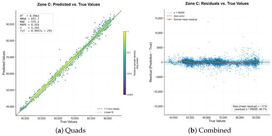
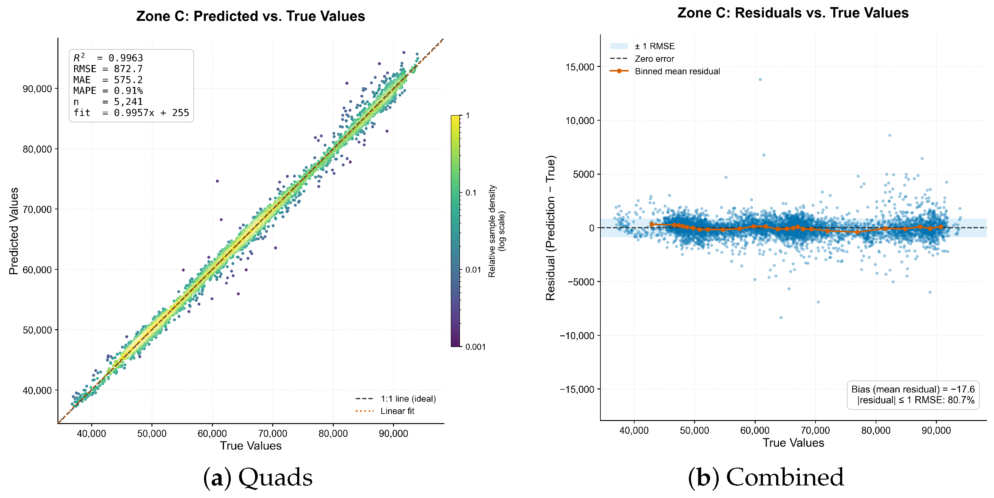
Figure 5 illustrates the corresponding results for Zone C. The scatter points are similarly concentrated around the 1:1 reference line, and the linear regression equation is $\widehat{y}=0.9957x+255$. The model achieves an $R^2$ of 0.9963, an RMSE of 872.7, an MAE of 575.2, and a MAPE of 0.91% across 5241 test samples. The regression slope is also close to 1, indicating strong agreement between predicted and actual loads. The residuals fluctuate around zero, and the binned mean residual curve remains close to the zero-error line across most of the load range. The mean residual is −17.6, indicating limited overall bias. Approximately 80.7% of the samples have residuals within $\pm 1$ RMSE, suggesting a relatively concentrated residual distribution. A small number of outliers appear around load levels of 60,000 and 80,000, potentially associated with abrupt load fluctuations or isolated variations in the observations.

Figure 5. Scatter plots of predicted and actual load values of Zone c.

Overall, Figure 4 and Figure 5 demonstrate that the model achieves high forecasting accuracy and limited overall bias in both zones. Although Zone C has substantially higher load levels and larger absolute errors, its MAPE is lower than that of Zone 1 (0.91% versus 0.99%), indicating slightly better relative forecasting accuracy. Moreover, the proportion of residuals within $\pm 1$ RMSE is slightly higher for Zone C than for Zone 1. These findings suggest that the model maintains consistent predictive performance across the two zones despite differences in their load magnitudes, although a small number of larger errors remain in the high-load regions.

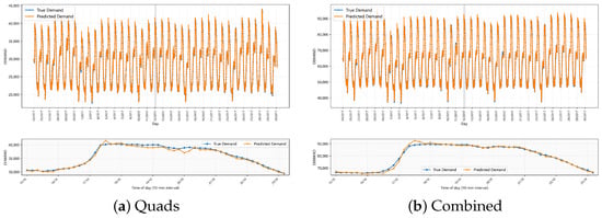
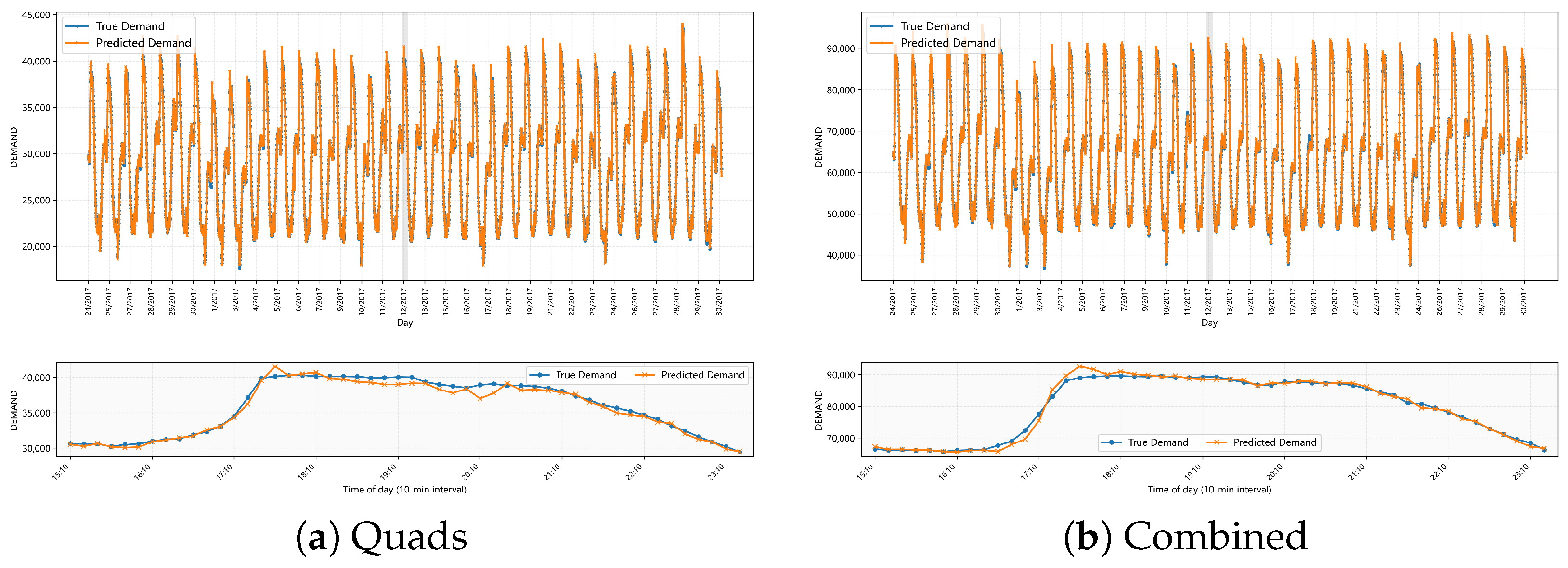
Figure 6 illustrates the actual and predicted electricity load curves under the Quads and Combined scenarios. The enlarged peak segments provide a closer view of the prediction behavior during abrupt load variations, allowing potential discrepancies between the predicted and actual load values to be examined in greater detail. As shown in the zoomed subplots, both models can generally capture the overall fluctuation trend of electricity load. However, noticeable deviations emerge at peak values, especially during sharp load drops.

Figure 6. Comparison of actual and predicted loads on the test set.

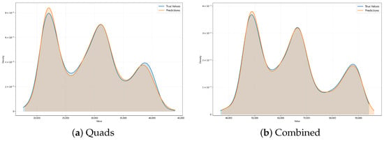
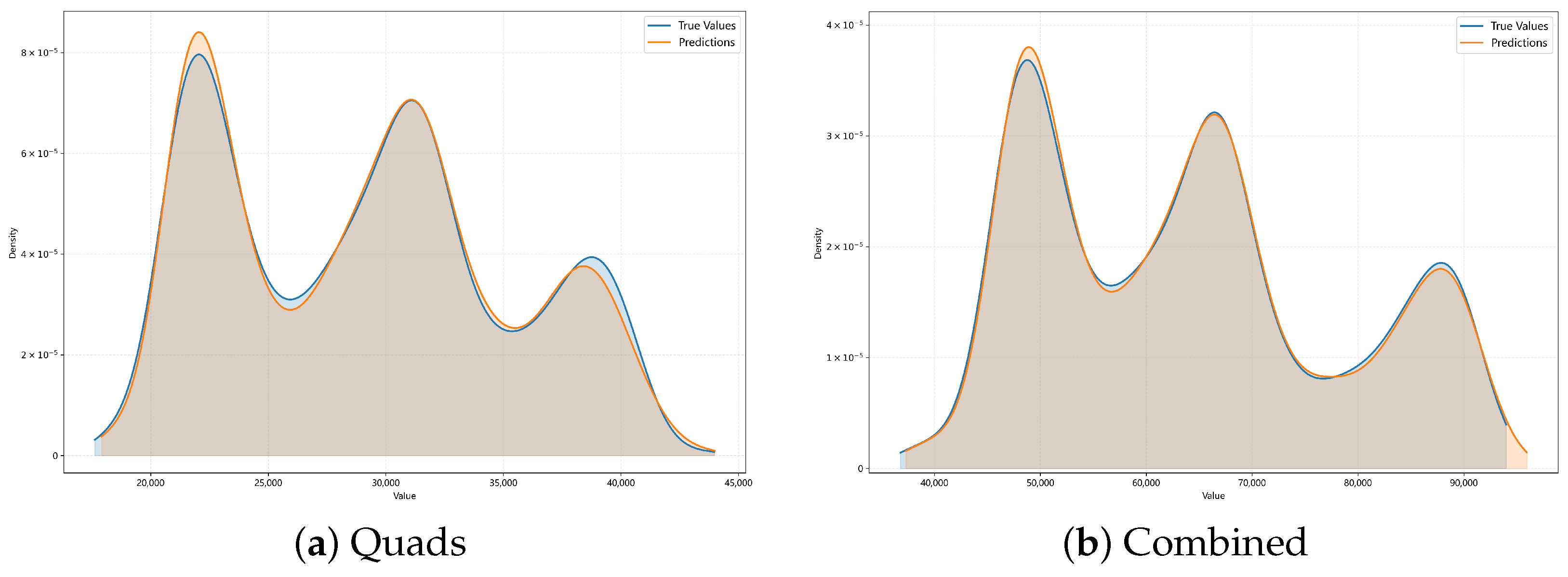
To further examine the statistical distributions of the forecasting results, Figure 7 presents the kernel density estimation (KDE) distributions of the actual and predicted load values. In both scenarios, the predicted and actual distributions show similar overall shapes and density patterns. This suggests that the predicted values reproduce the main marginal distribution characteristics of the actual load data. However, the KDE comparison reflects distribution-level similarity rather than pointwise forecasting accuracy.

Figure 7. KDE distributions of actual and predicted loads.

Table 1 summarizes the quantitative forecasting results of CNN-KAN under the two scenarios. For the Quads scenario, the model achieves an MSE of 175,755.7503, an RMSE of 419.2323, an MAE of 288.3134, an $R^2$ of 0.9954, and a MAPE of 0.9939%. For the Combined scenario, the corresponding values are 680,007.6, 824.6257, 592.0004, 0.9965, and 0.9256%, respectively. The $R^2$ values exceed 0.99 in both scenarios, while the MAPE values remain below 1%. These results indicate that CNN-KAN achieves stable forecasting performance under both load aggregation scenarios.

Table 1. Prediction performance of CNN-KAN under different forecasting scenarios.

Forecasting Scenario	MSE	RMSE	MAE	${\mathit{R}}^2$	MAPE (%)
Quads	175,755.7503	419.2323	288.3134	0.9954	0.9939
Combined	680,007.6271	824.6257	592.0004	0.9965	0.9256

4.4. Comparison with Baseline Models

To further evaluate the forecasting performance of the proposed CNN-KAN model, Decision Tree and LSTM are selected as baseline models for comparison. To provide a more comprehensive evaluation, two additional deep learning models, TCN and Informer, are included to represent temporal convolutional networks and Transformer-based time-series forecasting methods, respectively. All models use the same data preprocessing procedure and the same training, validation, and test sample splits as CNN-KAN to ensure consistency in model performance comparison. Experiments are conducted under both the Quads and Combined forecasting scenarios. Five evaluation metrics, including MSE, RMSE, MAE, $R^2$, and MAPE, are used for comprehensive evaluation. The results are shown in Table 2.

Table 2. Performance comparison of different models under different forecasting scenarios.

Forecasting Scenario	Method	MSE	RMSE	MAE	${\mathit{R}}^2$	MAPE (%)
Quads	Decision Tree	348,513.9185	590.3507	395.7367	0.9908	1.3633
	LSTM	178,267.1250	422.2174	332.9130	0.9953	1.1972
	TCN	185,742.7344	430.9788	290.5575	0.9949	1.0123
	Informer	222,750.5781	471.9646	324.9550	0.9939	1.1033
	CNN-KAN	175,755.7503	419.2323	288.3134	0.9954	0.9939
Combined	Decision Tree	851,954.3402	923.0137	653.1059	0.9958	1.0495
	LSTM	1,733,882.3722	1316.7697	1175.0533	0.9915	2.0179
	TCN	693,450.6875	832.7369	579.0229	0.9964	0.9103
	Informer	680,817.5625	825.1167	624.9204	0.9965	0.9913
	CNN-KAN	680,007.6271	824.6257	592.0004	0.9965	0.9256

Under the Quads scenario, CNN-KAN achieves the best results across all five evaluation metrics. Compared with LSTM, the MSE and RMSE of CNN-KAN decrease from 178,267.1250 and 422.2174 to 175,755.7503 and 419.2323, respectively, with relatively small differences between the two models. In contrast, the MAE decreases from 332.9130 to 288.3134, and the MAPE decreases from 1.1972% to 0.9939%, corresponding to reductions of approximately 13.40% and 16.98%, respectively. Meanwhile, the $R^2$ of CNN-KAN is 0.9954, slightly higher than the 0.9953 obtained by LSTM. Compared with Decision Tree, CNN-KAN also shows clear advantages in all error metrics, with MAPE decreasing from 1.3633% to 0.9939%. Compared with the newly introduced TCN and Informer models, CNN-KAN also achieves lower values across all four error metrics and a higher $R^2$. Specifically, its MAPE of 0.9939% is lower than the 1.0123% obtained by TCN and the 1.1033% obtained by Informer, corresponding to relative reductions of approximately 1.82% and 9.91%, respectively. Therefore, under the Quads scenario, CNN-KAN achieves MSE and RMSE values close to those of LSTM, while showing more obvious advantages in MAE and MAPE. These results further demonstrate its competitive forecasting performance against both recurrent and advanced deep learning time-series models under this scenario.

Although the MSE improvement of CNN-KAN over LSTM is relatively modest under the Quads scenario, model performance should be assessed using multiple complementary metrics rather than MSE alone. In this study, particular attention is given to MAPE because it expresses forecasting errors in relative terms. CNN-KAN achieves a MAPE of 0.9939%, compared with 1.1972% for LSTM, corresponding to a relative reduction of approximately 17.0%. CNN-KAN also obtains lower RMSE and MAE values. These results indicate that the observed performance advantage is not limited to MSE. Nevertheless, since the reported baseline comparison is based on point estimates, the statistical significance of the differences has not been established.

Under the Combined scenario, CNN-KAN achieves the lowest MSE and RMSE among the five models, with values of 680,007.6271 and 824.6257, respectively. Compared with Decision Tree, its MSE decreases from 851,954.3402 to 680,007.6271, RMSE decreases from 923.0137 to 824.6257, MAE decreases from 653.1059 to 592.0004, and MAPE decreases from 1.0495% to 0.9256%. Compared with LSTM, CNN-KAN also achieves substantially lower MSE, RMSE, MAE, and MAPE, while $R^2$ increases from 0.9915 to 0.9965. Compared with Informer, CNN-KAN produces slightly lower MSE and RMSE, although the differences are small: the MSE decreases from 680,817.5625 to 680,007.6271, and the RMSE decreases from 825.1167 to 824.6257. However, CNN-KAN does not achieve the best results across all metrics in this scenario. TCN obtains the lowest MAE of 579.0229 and the lowest MAPE of 0.9103%, outperforming CNN-KAN on these two metrics. It is also worth noting that the error metrics of LSTM increase markedly under the Combined scenario compared with the Quads scenario, whereas CNN-KAN still maintains $R^2>0.99$ and MAPE $<1\%$. This indicates that CNN-KAN can adapt well to the forecasting task under the aggregated load scenario.

Overall, compared with the Decision Tree and LSTM baseline models, CNN-KAN achieves better forecasting performance across the two forecasting scenarios. The additional comparisons with TCN and Informer provide a broader assessment of its performance against convolution-based and Transformer-based time-series forecasting methods. CNN-KAN achieves the best results across all five evaluation metrics under the Quads scenario. Under the Combined scenario, it obtains the lowest MSE and RMSE, while TCN performs better in terms of MAE and MAPE. These findings suggest that the relative performance of the models depends on the forecasting scenario and evaluation metric. Rather than demonstrating universal superiority, the results indicate that CNN-KAN offers competitive forecasting performance, with particularly strong results in the Quads scenario and in MSE and RMSE under the Combined scenario.

4.5. Ablation Study and Computational Cost Analysis

To investigate the contributions of different model components and evaluate the computational overhead introduced by the proposed B-spline KAN mechanism, three model configurations are compared: CNN, CNN + Original KAN, and CNN + B-spline KAN. The CNN baseline consists of a CNN feature extractor followed by a single-layer linear regression head. In the second configuration, the linear regression head is replaced with the original KAN architecture. The third configuration incorporates the proposed B-spline KAN mechanism, which employs recursively smoothed soft B-spline basis functions for nonlinear function approximation. The forecasting performance and computational costs of these configurations are evaluated using the same experimental dataset.

4.5.1. Ablation Study

Table 3 presents the forecasting performance of the three model configurations. The CNN baseline achieves an MSE of 234,678.39, an RMSE of 484.44, an MAE of 323.82, an $R^2$ of 0.9938, and a MAPE of 1.0935%. After replacing the linear regression head with the original KAN architecture, the MSE increases to 240,325.55, while the RMSE, MAE, and MAPE also increase. Meanwhile, $R^2$ decreases from 0.9938 to 0.9934. These results indicate that introducing the original KAN architecture does not automatically improve forecasting performance under the current experimental setting.

Table 3. Ablation study and computational cost comparison of different model configurations.

Model	MSE	RMSE	MAE	${\mathit{R}}^2$	MAPE (%)	Params (K)	Epochs	Train (s)	Inference (ms/Sample)
CNN	234,678.39	484.44	323.82	0.9938	1.0935	8.18	259	393.94	0.0257
CNN + Original KAN	240,325.55	490.23	328.01	0.9934	1.1200	14.49	260	1477.51	0.0795
CNN + B-spline KAN	198,204.03	445.20	310.12	0.9948	1.0726	16.06	168	1610.71	0.0852

In contrast, the CNN + B-spline KAN configuration achieves the best results across all five evaluation metrics, with an MSE of 198,204.03, an RMSE of 445.20, an MAE of 310.12, an $R^2$ of 0.9948, and a MAPE of 1.0726%. Compared with the CNN baseline, the proposed configuration reduces MSE by approximately 15.54%, RMSE by 8.10%, MAE by 4.23%, and MAPE by 1.91%, while increasing $R^2$ by 0.0010. Compared with the original KAN configuration, the MSE decreases by approximately 17.53%, and the RMSE decreases by approximately 9.18%.

These results demonstrate that the performance improvement does not arise simply from replacing the linear regression head with a KAN architecture. Instead, the B-spline KAN configuration provides more favorable forecasting performance than both the CNN baseline and the original KAN configuration. This finding supports the effectiveness of the proposed B-spline KAN design in the evaluated forecasting task. However, because the comparison involves complete model configurations, the observed improvement should be attributed to the overall B-spline KAN configuration rather than exclusively to the recursive smoothing mechanism.

In addition to forecasting accuracy, Table 3 reports the parameter counts and computational costs of the three model configurations. The CNN baseline contains 8.18 K trainable parameters, whereas the CNN + Original KAN and CNN + B-spline KAN configurations contain 14.49 K and 16.06 K parameters, respectively. Compared with the CNN baseline, these configurations introduce 6.31 K (77.14%) and 7.88 K (96.33%) additional parameters, respectively. The CNN + B-spline KAN configuration also requires longer training time (1610.71 s) and higher inference latency (0.0852 ms/sample) than the CNN baseline (393.94 s and 0.0257 ms/sample). Nevertheless, it achieves lower forecasting errors and converges in fewer epochs (168 versus 259). These results indicate that the B-spline KAN configuration improves forecasting accuracy at the cost of increased model complexity and computational time. Therefore, its practical suitability depends on the trade-off between prediction accuracy and computational efficiency.

4.5.2. Computational Cost Analysis

In addition to forecasting accuracy, the computational costs of the three configurations are evaluated in terms of the number of trainable parameters, total training time, and average per-sample inference time. The results are summarized in Table 3.

The CNN baseline contains 8.18 K trainable parameters and requires 393.94 s to complete training, with an average inference time of 0.0257 ms per sample. Incorporating the original KAN increases the parameter count to 14.49 K, the training time to 1477.51 s, and the inference time to 0.0795 ms per sample. The CNN + B-spline KAN configuration contains 16.06 K trainable parameters and requires 1610.71 s for training, with an average inference time of 0.0852 ms per sample.

Compared with the CNN baseline, the CNN + B-spline KAN configuration increases the number of trainable parameters by approximately 96.33%, the total training time by 308.88%, and the inference time by 231.52%. Compared with the original KAN configuration, it introduces a further increase of approximately 10.83% in parameter count, 9.01% in total training time, and 7.17% in inference time. These results quantitatively confirm that the B-spline KAN configuration incurs additional computational costs.

Notably, the B-spline KAN configuration converges in 168 training epochs, compared with 259 epochs for the CNN baseline and 260 epochs for the original KAN configuration. Nevertheless, its total training time remains longer because the computational cost per training epoch is also affected by the operations required by the KAN module. Therefore, a reduction in the number of training epochs does not necessarily translate into a reduction in total training time.

Overall, the experimental results reveal a trade-off between forecasting accuracy and computational efficiency. The B-spline KAN configuration achieves the best forecasting performance among the evaluated models, but this improvement comes at the expense of increased parameter count, training time, and inference time. These findings provide a quantitative assessment of the computational overhead associated with the proposed model and clarify the relationship between its predictive benefits and computational requirements.

4.6. Repeated-Run Stability Analysis

To address the potential variability associated with random initialization and stochastic training, five independent runs of the proposed CNN-KAN model were conducted on the Quads dataset using different random seeds (42, 123, 2024, 7, and 2025). The experimental settings were kept consistent across runs to ensure a fair assessment of the model’s performance variability. The evaluation metrics included MSE, RMSE, MAE, $R^2$, and MAPE. The results of the five runs and their statistical summaries are presented in Table 4.

Table 4. Repeated-run results of the proposed CNN-KAN model on the Quads dataset.

Number	Seed	MSE	RMSE	MAE	${\mathit{R}}^2$	MAPE (%)
1	42	193,483.58	439.87	291.00	0.9949	0.9967
2	123	201,672.52	449.08	322.59	0.9947	1.1144
3	2024	190,818.73	436.83	305.07	0.9950	1.0645
4	7	231,839.31	481.50	312.01	0.9939	1.0809
5	2025	177,312.13	421.08	294.87	0.9953	1.0241
Mean	–	199,025.25	445.67	305.11	0.9947	1.0561
Std	–	21,024.89	22.24	11.69	0.0005	0.0462

As shown in Table 4, the proposed model achieved an average MSE of 199,025.25, an RMSE of 445.67, an MAE of 305.11, an $R^2$ of 0.99476, and a MAPE of 1.05612% across the five runs. Although the prediction errors varied to some extent across random seeds, the $R^2$ values remained above 0.993, while the MAPE values remained below 1.12%. These results indicate that the model maintained consistently strong predictive performance across repeated runs on the Quads dataset. Reporting the mean and standard deviation provides a more comprehensive evaluation of the model than relying on a single training run.

4.7. Parameter Sensitivity Analysis

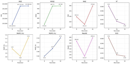
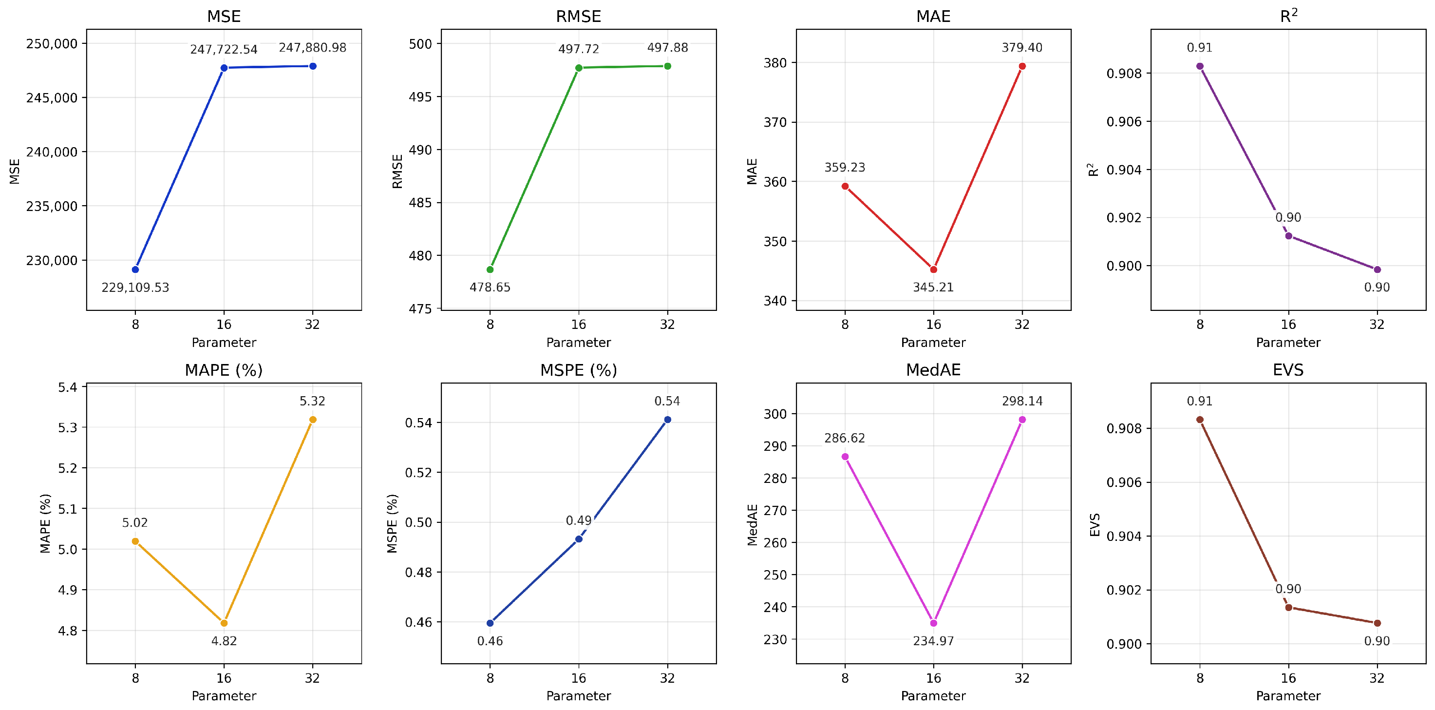
To analyze the effect of the sliding window length on the forecasting performance of CNN-KAN, three window lengths, $L=8$, $L=16$, and $L=32$, are evaluated under the Quads forecasting scenario. Comparative experiments are conducted while keeping the other model parameters and training settings unchanged. Figure 8 shows the changes in the evaluation metrics of the model under different window lengths.

Figure 8. Performance of CNN-KAN with different sliding window lengths.

The experimental results show that when the window length increases from 8 to 16 and 32, most evaluation metrics do not improve further. When the window length increases to 32, the overall forecasting performance decreases compared with that obtained at $L=8$. Considering MSE, RMSE, MAE, $R^2$, and MAPE, the model achieves the best performance when the window length is $L=8$. Considering the overall performance across the evaluation metrics, (L = 8) is selected for the subsequent experiments, although (L = 16) achieves lower MAE and NMAE.

A possible explanation is that the usefulness of historical observations depends on their relevance to the target time step rather than solely on the amount of historical information available. Under the current forecasting settings, the most recent eight time steps may already capture the dominant short-term load variations. Extending the window may introduce additional historical fluctuations with limited predictive value, potentially making it more difficult for the model to identify relevant patterns. Furthermore, the CNN branch extracts local patterns from the input sequence, while the KAN module performs subsequent nonlinear feature mapping. A longer input window may increase the complexity of the extracted representations without necessarily providing additional useful predictive information.

However, these explanations remain speculative, as the current experiments demonstrate performance differences across window lengths but do not directly establish their underlying causes. Therefore, (L = 8) is adopted as the final setting based on the overall evaluation results. This choice reflects the performance observed under the current dataset and forecasting settings, rather than implying that shorter input windows are universally preferable.

4.8. Discussion

The experimental results demonstrate that the proposed CNN-KAN framework can effectively model short-term electricity load variations under different load aggregation scenarios. The CNN module provides local temporal-feature representation by capturing short-term fluctuation patterns from multivariate load-related sequences, while the KAN module further enhances nonlinear feature mapping through the proposed recursive smoothing soft B-spline basis mechanism. The combination of these two components enables the model to learn complex relationships between historical load patterns and external environmental factors. The consistent performance observed in both Quads and Combined scenarios indicates that CNN-KAN can adapt to different load aggregation scales and maintain stable prediction capability under the current experimental settings. However, since no independent ablation study is conducted in this work, the specific contribution of each individual component requires further investigation.

Although the proposed method achieves promising prediction performance, several limitations remain. First, the experiments are conducted using the Tetouan City electricity load dataset, with the Quads and Combined scenarios derived from the same data source. Therefore, the current results primarily demonstrate the adaptability of CNN-KAN to different load aggregation scenarios rather than its generalization capability across geographical regions or climatic conditions.

Furthermore, the comparative results indicate that the relative performance of different models depends on the forecasting scenario and evaluation metric. Although CNN-KAN achieves the best results across all five evaluation metrics under the Quads scenario, TCN obtains lower MAE and MAPE values under the Combined scenario. This suggests that the advantages of CNN-KAN may vary with load aggregation characteristics and the evaluation metric considered.

Regarding the contribution of the KAN component, although the improvement in MAPE over the CNN baseline is relatively small in absolute terms, the proposed CNN-KAN model also reduces MSE and MAE, indicating improvements across multiple prediction error metrics. Therefore, the effectiveness of the proposed model should be evaluated by considering multiple performance indicators rather than MAPE alone. The comparative results further demonstrate that CNN-KAN achieves competitive forecasting performance across the Quads and Combined scenarios, supporting the potential of integrating CNN-based feature extraction with KAN-based nonlinear mapping for short-term electricity load forecasting. Meanwhile, further improvements in computational efficiency remain a worthwhile direction for future research.

Future studies will evaluate the proposed framework using electricity load datasets from more diverse geographical and climatic regions, as well as granular-level consumption datasets, such as household- and building-level load profiles, to further investigate its cross-region generalization capability and applicability to fine-grained load forecasting. In addition, future work will investigate the factors affecting model performance under different forecasting scenarios and explore more computationally efficient nonlinear feature representation and model optimization strategies. In particular, architectural optimization and more efficient basis function computation will be investigated to reduce the number of trainable parameters and training time while preserving predictive accuracy, thereby further improving the practical applicability of the proposed framework.

5. Conclusions

This paper proposes a CNN-KAN heterogeneous feature mapping framework for short-term electricity load forecasting. By integrating the local temporal-feature extraction capability of CNN and the nonlinear representation capability of KAN, the proposed framework establishes a serial feature transformation process from local pattern extraction to nonlinear feature reconstruction. Furthermore, a recursive smoothing soft B-spline basis mapping mechanism is introduced into the KAN module to enhance the continuity of basis responses and improve the flexibility of nonlinear feature representation.

Experiments conducted on the Tetouan City electricity load dataset demonstrate that the proposed CNN-KAN model achieves stable prediction performance under two load forecasting scenarios with different aggregation scales. The model obtains $R^2$ values higher than 0.99 and MAPE values lower than 1% in both Quads and Combined scenarios. Compared with Decision Tree and LSTM baseline models, CNN-KAN achieves better overall prediction performance, particularly in MAE and MAPE metrics. These results indicate that the proposed framework can effectively capture complex nonlinear relationships between historical load patterns and environmental factors, providing a reliable approach for short-term electricity load forecasting.

References

- Altinay, G.; Karagol, E. Electricity consumption and economic growth: Evidence from Turkey. Energy Econ. 2005, 27, 849–856. [Google Scholar] [CrossRef] [Scilit]
- Hong, T.; Fan, S. Probabilistic electric load forecasting: A tutorial review. Int. J. Forecast. 2016, 32, 914–938. [Google Scholar] [CrossRef] [Scilit]
- Jiang, P.; Li, R.; Liu, N.; Gao, Y. A novel composite electricity demand forecasting framework by data processing and optimized support vector machine. Appl. Energy 2020, 260, 114243. [Google Scholar] [CrossRef] [Scilit]
- Yalew, S.G.; van Vliet, M.T.; Gernaat, D.E.; Ludwig, F.; Miara, A.; Park, C.; Byers, E.; De Cian, E.; Piontek, F.; Iyer, G.; et al. Impacts of climate change on energy systems in global and regional scenarios. Nat. Energy 2020, 5, 794–802. [Google Scholar] [CrossRef] [Scilit]
- Antoniadou-Plytaria, K.; Eriksson, L.; Johansson, J.; Johnsson, R.; Kötz, L.; Lamm, J.; Lundblad, E.; Steen, D.; Tuan, L.A.; Carlson, O. Effect of short-term and high-resolution load forecasting errors on microgrid operation costs. In Proceedings of the 2022 IEEE PES Innovative Smart Grid Technologies Conference Europe (ISGT-Europe); IEEE: Piscataway, NJ, USA, 2022; pp. 1–5. [Google Scholar]
- Rabie, D.; Moradi, M.; Xuan, W.; Farzaneh, H. Impact of accurate load forecasting on electricity market stability in Japan using classical time-series and deep-learning methods. Sci. Rep. 2026, 16, 11781. [Google Scholar] [CrossRef] [Scilit] [PubMed]
- Hyndman, R.J.; Athanasopoulos, G. Forecasting: Principles and Practice; OTexts: Heathmont, VIC, Australia, 2018. [Google Scholar]
- Chen, J.F.; Wang, W.M.; Huang, C.M. Analysis of an adaptive time-series autoregressive moving-average (ARMA) model for short-term load forecasting. Electr. Power Syst. Res. 1995, 34, 187–196. [Google Scholar] [CrossRef] [Scilit]
- Momani, M.A.; Abwaini, R.K.; Ababneh, B.M.; Nasser, M.A. Comparative Analysis of ARIMA and SARIMA Models in Electrical Load Forecasting: Insights for Long and Short-Term Projections. Int. J. Electr. Eng. Comput. Sci. 2025, 7, 83–89. [Google Scholar] [CrossRef] [Scilit]
- Park, D.C.; El-Sharkawi, M.; Marks, R.; Atlas, L.; Damborg, M. Electric load forecasting using an artificial neural network. IEEE Trans. Power Syst. 2002, 6, 442–449. [Google Scholar]
- Chen, B.J.; Chang, M.W. Load forecasting using support vector machines: A study on EUNITE competition 2001. IEEE Trans. Power Syst. 2004, 19, 1821–1830. [Google Scholar] [CrossRef] [Scilit]
- Torres, J.F.; Hadjout, D.; Sebaa, A.; Martínez-Álvarez, F.; Troncoso, A. Deep learning for time series forecasting: A survey. Big Data 2021, 9, 3–21. [Google Scholar] [CrossRef] [Scilit] [PubMed]
- Ghimire, S.; Deo, R.C.; Casillas-Perez, D.; Salcedo-Sanz, S.; Acharya, R.; Dinh, T. Electricity demand uncertainty modeling with Temporal Convolution Neural Network models. Renew. Sustain. Energy Rev. 2025, 209, 115097. [Google Scholar] [CrossRef] [Scilit]
- Hasanah, R.N.; OMP, R.R.; Suyono, H. Comparison analysis of electricity load demand prediction using recurrent neural network (rnn) and vector autoregressive model (var). In Proceedings of the 2020 12th International Conference on Electrical Engineering (ICEENG); IEEE: Piscataway, NJ, USA, 2020; pp. 23–29. [Google Scholar]
- Muzaffar, S.; Afshari, A. Short-term load forecasts using LSTM networks. Energy Procedia 2019, 158, 2922–2927. [Google Scholar] [CrossRef] [Scilit]
- Liu, Z.; Wang, Y.; Vaidya, S.; Ruehle, F.; Halverson, J.; Soljačić, M.; Hou, T.Y.; Tegmark, M. Kan: Kolmogorov-arnold networks. arXiv 2024, arXiv:2404.19756. [Google Scholar]
- Long, Y.; Qin, X. A multivariate time series prediction model based on the KAN network. Sci. Rep. 2025, 15, 23621. [Google Scholar] [CrossRef] [Scilit] [PubMed]
- Lahouar, A.; Slama, J.B.H. Day-ahead load forecast using random forest and expert input selection. Energy Convers. Manag. 2015, 103, 1040–1051. [Google Scholar] [CrossRef] [Scilit]
- Ju, Y.; Sun, G.; Chen, Q.; Zhang, M.; Zhu, H.; Rehman, M.U. A model combining convolutional neural network and LightGBM algorithm for ultra-short-term wind power forecasting. IEEE Access 2019, 7, 28309–28318. [Google Scholar] [CrossRef] [Scilit]
- Yao, X.; Fu, X.; Zong, C. Short-term load forecasting method based on feature preference strategy and LightGBM-XGboost. IEEE Access 2022, 10, 75257–75268. [Google Scholar] [CrossRef] [Scilit]
- Zuo, C.; Wang, J.; Liu, M.; Deng, S.; Wang, Q. An ensemble framework for short-term load forecasting based on timesnet and tcn. Energies 2023, 16, 5330. [Google Scholar] [CrossRef] [Scilit]
- Zhao, Z.; Yun, S.; Jia, L.; Guo, J.; Meng, Y.; He, N.; Li, X.; Shi, J.; Yang, L. Hybrid VMD-CNN-GRU-based model for short-term forecasting of wind power considering spatio-temporal features. Eng. Appl. Artif. Intell. 2023, 121, 105982. [Google Scholar] [CrossRef] [Scilit]
- Zang, Y.; Zhao, Z.; Gao, J.; Wang, X.; Li, S.; Ma, Q.; Liu, M.; Wang, J. Time-Lag-Aware Redundancy-Constrained Feature Selection and VMD–LSTM Framework for Short-Term Load Forecasting. Energies 2026, 19, 3901. [Google Scholar] [CrossRef] [Scilit]
- Rafi, S.H.; Deeba, S.R.; Hossain, E. A short-term load forecasting method using integrated CNN and LSTM network. IEEE Access 2021, 9, 32436–32448. [Google Scholar] [CrossRef] [Scilit]
- Wang, Y.; Sun, J.; Bai, J.; Anitescu, C.; Eshaghi, M.S.; Zhuang, X.; Rabczuk, T.; Liu, Y. Kolmogorov–Arnold-Informed neural network: A physics-informed deep learning framework for solving forward and inverse problems based on Kolmogorov–Arnold Networks. Comput. Methods Appl. Mech. Eng. 2025, 433, 117518. [Google Scholar] [CrossRef] [Scilit]
- Mostajeran, F.; Faroughi, S.A. Scaled-cpikans: Spatial variable and residual scaling in Chebyshev-based physics-informed Kolmogorov-Arnold networks. J. Comput. Phys. 2025, 537, 114116. [Google Scholar] [CrossRef] [Scilit]
- fedesoriano. Electric Power Consumption Dataset. 2022. Available online: https://www.kaggle.com/datasets/fedesoriano/electric-power-consumption (accessed on 1 September 2026).
Disclaimer/Publisher’s Note: The statements, opinions and data contained in all publications are solely those of the individual author(s) and contributor(s) and not of MDPI and/or the editor(s). MDPI and/or the editor(s) disclaim responsibility for any injury to people or property resulting from any ideas, methods, instructions or products referred to in the content. |
© 2026 by the authors. Licensee MDPI, Basel, Switzerland. This article is an open access article distributed under the terms and conditions of the Creative Commons Attribution (CC BY) license.