Electric-Field-Based Reconstruction of Transmission-Line Galloping Characteristics Using an Arc-Length Constraint

Abstract

Conductor galloping threatens the safe operation of overhead transmission lines, motivating non-contact methods for reconstructing its motion characteristics. However, recovering conductor displacement from electric-field measurements near the suspension point requires resolving the coupled effects of deflection and sag. This study develops an electric-field-based reconstruction method that combines local angle inversion with an arc-length constraint. A three-dimensional conductor model relates the tangential deflection angles to multipoint electric-field observations, and relative amplitude measurements provide the inputs for local Jacobian inversion. The reconstructed angles are combined with prescribed spatial modes and the inextensibility constraint to obtain horizontal and vertical displacement components while accounting for sag variation. Spectral analysis of the reconstructed motion sequences extracts the dominant frequencies. The observation model is further extended to three-phase electric-field superposition with known relative phase-voltage magnitudes and phases. Controlled single-conductor laboratory tests evaluate displacement reconstruction against scale references, while separate known-input numerical comparisons assess angle, displacement, and frequency recovery. Error analyses examine the effects of measurement perturbations, geometric uncertainty, and observation sensitivity on reconstruction. The results support recovery of the overall imposed motion patterns while identifying direction-dependent deviations and sensitivity to low-amplitude inputs. The method provides a basis for reconstructing conductor galloping characteristics from local electric-field measurements under specified geometric and measurement conditions.

1. Introduction

Overhead transmission lines are essential components of modern power systems and play a fundamental role in maintaining reliable and sustainable electricity supply. However, their safe operation can be significantly affected by conductor galloping, a low-frequency (0.1–3 Hz) and large-amplitude aeroelastic oscillation that is commonly associated with asymmetric ice accretion under winter weather conditions. Galloping can result in phase-to-phase flashovers, conductor fatigue, hardware damage, insulator string failure, and, in severe cases, tower collapse, thereby posing a considerable threat to transmission system reliability [1,2]. The occurrence and development of galloping are influenced by multiple factors, including the evolving geometry of ice accretion, fluctuating wind conditions, and the mechanical properties of transmission-line components, which increase the difficulty of accurate prediction and effective prevention [3,4]. In addition, recent wind-tunnel experiments have shown that unsteady wind excitation can produce larger galloping amplitudes than equivalent steady-wind conditions and can reduce the critical wind speed required for galloping initiation [1,3]. The resulting mechanical and electrical effects can accumulate over different time scales: large conductor motion may cause phase-to-phase flashovers, repeated bending may accelerate material degradation, and excessive longitudinal loads may contribute to structural damage or tower failure [2,5]. Therefore, considering the rapid evolution and multi-factor nature of conductor galloping, reliable and continuous monitoring is important for the timely identification of abnormal conductor motion and for improving the operational resilience of overhead transmission lines.

Contact-based monitoring is one of the established approaches for conductor galloping detection, in which sensors are physically attached to the conductor or tower to obtain mechanical response information. Accelerometer-based systems measure conductor acceleration at the attachment point, while modern MEMS sensors provide high sensitivity and low power consumption, facilitating their integration with wireless sensor networks [6,7]. Fiber Bragg grating (FBG) sensors provide another approach by enabling continuous measurement of strain and temperature along optical fibers, while offering immunity to electromagnetic interference in high-voltage environments [8,9,10]. To address the power requirements of sensors deployed in remote transmission corridors, triboelectric–electromagnetic hybridized modules have also been investigated to harvest energy from conductor motion and support self-powered monitoring [11,12]. Despite these developments, contact-based methods still involve practical considerations in field deployment. Sensor installation on conductors may require line outages or specialized live-line operations, while the additional sensor mass can influence the local dynamic characteristics of the conductor. Long-term operation also requires consideration of sensor maintenance and environmental exposure. Moreover, measurements obtained at discrete locations provide local motion information and may not fully represent the spatial characteristics of galloping along the conductor [6,8]. These considerations have encouraged the exploration of non-contact sensing approaches that can reduce installation requirements while providing continuous information on conductor motion.

The practical considerations associated with contact-based monitoring have also motivated the development of non-contact sensing approaches. Vision-based methods, including stereo-vision and monocular camera systems combined with deep learning-based image processing, can reconstruct conductor trajectories without physical attachment. Recent image segmentation frameworks, such as SAM2, have further improved the accuracy of conductor tracking [13,14,15]. However, their measurement performance can be affected by fog, rain, snow, illumination, and other environmental conditions, while real-time image processing may require considerable computational resources [16,17,18].

Electromagnetic sensing provides another non-contact approach by utilizing the electric and magnetic fields surrounding energized conductors. Magnetic measurements have been used for contactless current and sag monitoring under practical engineering conditions [19], while magnetic sensor arrays have been developed for simultaneous monitoring of current and conductor galloping [20]. Electric-field-based methods have also been investigated for non-contact conductor sag measurement [21]. Related work on non-contact voltage reconstruction addresses dual-pin probe structures and measurement-point optimization for overhead transmission lines [22]. Ground-based magnetic sensor arrays have also been developed to estimate three-phase currents without direct attachment to conductors [23]. In addition, electromagnetic sensing has been combined with optical components, such as a laser diode-in-capacitors structure, for simultaneous monitoring of voltage, electromagnetic interference, and vibration [24]. Non-contact traveling-wave measurements provide another sensing modality, in which conductor motion can be reflected in changes in wave propagation characteristics [25].

Compared with contact-based and vision-based approaches, electromagnetic sensing offers the advantages of non-contact deployment and continuous measurement, while avoiding direct dependence on optical visibility. Nevertheless, converting field measurements into conductor motion requires accounting for conductor position, electrical operating conditions, and the surrounding electromagnetic environment. For the present electric-field-based reconstruction, the geometric observation model and parameter-decoupling procedure therefore form the link between near-field measurements and conductor spatial motion.

Table 1 compares the monitoring approaches discussed above.

Table 1. Comparative evaluation of transmission-line galloping monitoring methods.

Monitoring Method	Deployment Invasiveness	Measurement Fidelity	Weather Robustness	Spatial Coverage	Cost	Reference
MEMS accelerometer	High (clamp-on)	High	Moderate	Point only	Moderate	[6]
FBG tension sensor	High (bonded fiber)	High	High	Distributed	High	[8,9]
Stereo-vision camera	None	Moderate	Low (fog/rain)	Full span	Moderate	[13,15]
Magnetic-field sensing	None	Moderate	High	Full span	Low	[19,20]
Electric-field sensing	None	High	High	Full span	Low	[21]

When conductor galloping occurs, its spatial position changes continuously, resulting in corresponding variations in the surrounding electric field. These variations are reflected in both the temporal and spatial characteristics of the measured electric-field signals. In the time domain, the field exhibits periodic or quasi-periodic variations associated with conductor motion, while in the spatial domain, the field intensity and potential differences vary with the relative positions of the conductor and measurement points. This relationship provides a physical basis for inferring conductor motion from non-contact near-field electric-field measurements.

Based on this principle, this study focuses on a single-phase conductor and develops a near-field spatial electric-field-based method for conductor galloping monitoring. Starting from the three-dimensional geometry of the conductor near the suspension point, the spatial electric-field distribution and its variation with conductor position are analyzed. The inverse relationship between electric-field measurements and conductor deflection is then established, with the inextensibility constraint introduced to obtain the corresponding displacement components. The main work of this study is as follows:

1. A near-field spatial electric-field model is established to characterize the relationship between conductor position and measured electric-field quantities.

2. A geometric inversion method is developed to obtain the conductor deflection angles and corresponding vertical and horizontal displacement components from multipoint electric-field measurements.

3. The inverted motion signals are processed to extract the dominant frequency and displacement variation characteristics, providing a basis for conductor galloping identification and monitoring.

2. Conductor Galloping Detection Using Near-Field Electric-Field Sensing

This method reconstructs conductor motion from near-field electric measurements obtained by sensors installed near the suspension point. The single-conductor geometric response and local inversion are developed first. A three-phase extension then incorporates the known relative voltage magnitudes and phases into a joint spatial observation model.

2.1. Three-Dimensional Spatial Modeling of Transmission Conductors

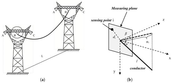
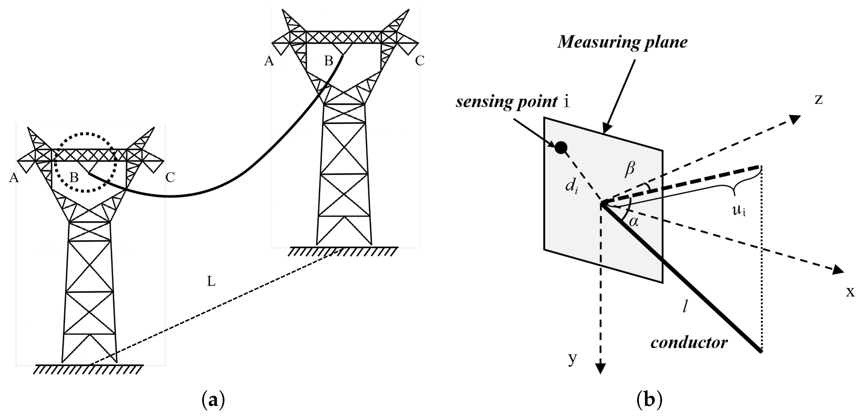
In the proposed model, the transmission conductor cannot be simplified as an infinitely long straight wire. In its static state, both ends are suspended from the tower insulator strings, and its spatial profile follows a catenary distribution governed by the combined effects of gravity and axial tension. A three-dimensional Cartesian coordinate system is established by designating the conductor suspension point as the origin, where the direction along the conductor line at the suspension point is defined as the z-axis, the direction perpendicular to the ground as the y-axis, and the direction perpendicular to the conductor as the x-axis. Accordingly, the spatial coordinates of any point on the conductor can be formulated as follows:

$$\left\{\begin{array}{cc}\hfill x& =l\cos \alpha \sin \beta \hfill \\ \hfill y& =l\sin \alpha \hfill \\ \hfill z& =l\cos \alpha \cos \beta \hfill \end{array}\right.$$

(1)

where l denotes the length of the conductor from the starting point of the tower insulator string to a specific point on the conductor, $\alpha$ is the vertical deflection angle of the conductor, and $\beta$ represents the horizontal deflection angle of the conductor, as illustrated in Figure 1.

Figure 1. (a) Schematic diagram of the overhead conductor. (b) Schematic diagram of the measurement plane at the suspension point.

Under the combined effects of ice accretion and wind loads, the conductor will experience complex multi-modal galloping, and its instantaneous three-dimensional spatial profile can be regarded as a multi-order low-frequency standing wave. To simplify the extraction of the macroscopic dominant characteristics of galloping, the galloping mode perpendicular to the conductor direction is defined as the $n_x$-th order galloping, with an instantaneous maximum amplitude (antinode) of $A_x\left(t\right)$; and the galloping mode perpendicular to the ground is defined as the $n_y$-th order galloping, with an instantaneous maximum amplitude (antinode) of $A_y\left(t\right)$. Its instantaneous dynamic spatial equations are defined as:

$$\left\{\begin{array}{cc}\hfill X(z,t)& =A_x\left(t\right)\sin \left({\displaystyle \frac{n_x\pi z}{L}}\right)\hfill \\ \hfill Y(z,t)& =-{\displaystyle \frac{4f_{sag}\left(t\right)}{L^2}}z(L-z)+A_y\left(t\right)\sin \left({\displaystyle \frac{n_y\pi z}{L}}\right)\hfill \\ \hfill Z(z,t)& =z\hfill \end{array}\right.$$

(2)

The high axial stiffness of aluminum conductor steel-reinforced (ACSR) conductors motivates the inextensibility approximation. Under this assumption, the total conductor arc length $S_0$ remains constant during motion, while the transient sag varies with the displacement components. Substituting the spatial derivatives of the conductor profile into the curve-length integral gives the following expression for $S_0$.

$$S_0={\int }_0^L\sqrt{1+{\left[X^{\prime }(z,t)\right]}^2+{\left[Y^{\prime }(z,t)\right]}^2}\mathrm{d}z$$

(3)

Since the ratio of the sag to the span length of the overhead conductor, $f_{sag}/L$, is typically around 4%, and the conductor slope of the first-order galloping, which exhibits the maximum amplitude during the galloping process, is much less than one, let:

$$u={\left[X^{\prime }(z,t)\right]}^2+{\left[Y^{\prime }(z,t)\right]}^2\ll 1$$

(4)

Using a Maclaurin series expansion of $\sqrt{1+u}$ about $u=0$ and retaining terms through first order gives $\sqrt{1+u}\approx 1+u/2$ for $u\ll 1$.

$$\sqrt{1+u}\approx 1+{\displaystyle \frac{u}{2}}$$

(5)

The shallow-slope expansion retains the mixed term between the static parabolic profile and the vertical sinusoidal component. This term generally does not vanish for odd vertical orders.

$$S_0\approx L+{\displaystyle \frac{8f_{sag}^2}{3L}}+{\displaystyle \frac{{\pi }^2}{4L}}(n_y^2{A}_y^2+n_x^2{A}_x^2)-{\displaystyle \frac{8f_{sag}{A}_y}{n_y\pi L}}\left[1-{(-1)}^{n_y}\right].$$

(6)

2.2. Measurement of Conductor Spatial Characteristics Using Near-Field Electric-Field Sensing

The distribution of the spatial electrostatic field maintains a direct physical correlation with the geometric positional variations of the transmission conductor. Equation (7) elucidates the electric-field intensity generated by a point charge with a charge quantity of q at a spatial distance of r:

$$E\left(r\right)={\displaystyle \frac{q}{4\pi {\epsilon }_0{r}^2}}$$

(7)

where ${\epsilon }_0$ represents the permittivity of vacuum, and the distance $r_i\left(z\right)$ from a specific point on the actual conductor to the measurement point is defined as:

$$r_i\left(z\right)=\sqrt{{[x_i-x\left(z\right)]}^2+{[y_i-y\left(z\right)]}^2+{(z_i-z)}^2}$$

(8)

Consequently, the electric potential generated by a point charge at a distance r can be derived as:

$$\phi ={\displaystyle \frac{q}{4\pi {\epsilon }_{0}r}}$$

(9)

The span is divided into a measurement-dominant conductor segment near the suspension point, $[0,L_e]$, and the remaining segment, $(L_e,L]$. Here, $L_e$ is the effective observation length. The tangent approximation is used for the local analytical response. Contributions from the remaining conductor and the adopted boundaries are included in the forward model rather than identified with an arbitrary potential-zero shift.

Within the measurement-dominant segment near the suspension point, the analytical model approximates the conductor locally by its spatial tangent. According to Equation (1), $\alpha$ is the vertical elevation angle and $\beta$ the horizontal deflection angle. The local approximation is evaluated together with the adopted observation length and boundary response.

Substituting the spatial coordinates into the distance function $r_i\left(l\right)$ from the measurement point to the conductor infinitesimal element yields:

$$r_i\left(l\right)=\sqrt{{(x_i-l\cos \alpha \sin \beta )}^2+{(y_i-l\sin \alpha )}^2+{(z_i-l\cos \alpha \cos \beta )}^2}$$

(10)

Expanding the brackets and collecting like terms, this distance function can be expressed as a standard quadratic form concerning the infinitesimal arc length l:

$$r_i\left(l\right)=\sqrt{l^2-2u_i(\alpha ,\beta )l+d_i^2}$$

(11)

$$d_i=\sqrt{x_i^2+y_i^2+z_i^2}$$

(12)

$$u_i=x_i\cos \alpha \sin \beta +y_i\sin \alpha +z_i\cos \alpha \cos \beta$$

(13)

Herein, two functions are defined: The first is $d_i$, which acts as the linear distance constant from the spatial measurement point $P_i$ to the coordinate origin. The second is $u_i$, which physically represents the geometric projection length of the measurement point position vector onto the instantaneous spatial unit tangent directional vector of the conductor. It correlates the unknown transient deflection angles $\alpha$ and $\beta$ with the known spatial coordinates of the sensors.

Substituting the distance function into Equation (9) gives the analytical response of the local straight segment. The term $C_i$ retains contributions from the remaining conductor and the adopted image-charge boundaries under the fixed potential reference. Its treatment must be consistent with the measurement model and normalization.

$$\begin{array}{cc}\hfill {\phi }_i& ={\displaystyle \frac{\lambda }{4\pi {\epsilon }_0}}{\int }_0^{L_e}{\displaystyle \frac{1}{\sqrt{l^2-2u_{i}l+d_i^2}}}\mathrm{d}l+C_i={\displaystyle \frac{\lambda }{4\pi {\epsilon }_0}}\ln {\displaystyle \frac{L_e-u_i+\sqrt{L_e^2-2u_i{L}_e+d_i^2}}{d_i-u_i}}+C_i\hfill \end{array}$$

(14)

Here $\lambda$ is the conductor charge per unit length. If $L_e\gg d_i$ and $L_e\gg \left|u_i\right|$, the local segment contribution admits the following approximation. Boundary and remaining-conductor terms are retained in $C_i$.

$${\phi }_i\approx {\displaystyle \frac{\lambda }{4\pi {\epsilon }_0}}[\ln \left(2L_e\right)-\ln (d_i-u_i)]+C_i$$

(15)

The measured signal is the AC-coupled difference between the two probe-induced voltages. The alternating power-frequency carrier amplitude is extracted from the conditioned output. The V- probe serves as the differential comparison electrode, not a directly grounded reference electrode. Board GND connects to site ground through the cable’s grounding conductor; this node is the 0 V reference. The INA821 REF, downstream offset reference Vref, and ADC conversion reference REF_2.5V serve their respective circuit functions and do not constitute one spatial-potential zero. Ratiometric observations use effective alternating amplitudes corresponding to the probe response and channel transfer relation, excluding the output DC operating level. The field model adopts a fixed potential-reference convention and maps field quantities to these observations through the probe response.

Under a fixed measurement reference, the forward relation must include probe coupling, differential response, and channel transfer characteristics, and must predict the effective alternating amplitude. Only shared multiplicative source-amplitude factors cancel in a ratio; unmatched gain, additive background, and contributions from other phases require separate treatment. Physical contributions from distant conductor segments and image charges are not arbitrary potential-zero shifts. Terms entering a normalized expression require consistent dimensional normalization.

Table 2 summarizes the measured quantities and reference connections.

Table 2. Measured quantities and reference connections.

Item	Measured Quantity or Reference	Connection, Potential and Scope
Reference electrode	V- probe is the differential comparison electrode; both probes sense the field.	Both inputs are AC-coupled; no separate directly grounded reference electrode is specified.
Ground potential	Board GND connects through the sensor cable’s grounding conductor to site ground, taken as the 0 V reference.	INA821 REF connects to GND; AGND connects through a ferrite bead. The reference node defines 0 V.
Shield connections	The grounding conductor is distinct from a shield. Sensing probes are not grounded electrodes.	Site ground connects through the cable’s grounding conductor. Separate shield and enclosure grounding connections are not shown.
Transfer function	Nominal probe-voltage-difference to analog-output response is the product of AC coupling, differential gain, both bandpass stages and PGA response.	Nominal 50 Hz gain is approximately 38.91 × PGA gain; -3 dB passband 44.83–53.75 Hz. Probe loading and digital-window response are included separately.
Measured quantity	Probe-induced voltages undergo differential amplification; effective alternating amplitudes form the ratios.	The DC level is excluded. Vref sets output bias; REF_2.5V is the ADC conversion reference.

Ratios are formed from effective alternating amplitudes after probe and channel-response correction. The equations below first describe the point-potential forward model under a fixed reference; its ratio is mapped to the measured differential-amplitude ratio through the probe response.

$$R_{ij}={\displaystyle \frac{{\phi }_i}{{\phi }_j}}$$

(16)

Let $K=\lambda /\left(4\pi {\epsilon }_0\right)$ and $g_i=\ln \left(2L_e\right)-\ln (d_i-u_i)$. Under the fixed reference, the ratio is

$$R_{ij}(\alpha ,\beta )={\displaystyle \frac{K{g}_i(\alpha ,\beta )+C_i}{K{g}_j(\alpha ,\beta )+C_j}}.$$

(17)

A common multiplicative source factor cancels when the additive terms are negligible, removed consistently, or scale with the same factor. Additive background, unmatched channel response and other phases are retained in their corresponding measurement models.

When selecting the intrinsic vertical elevation angle ${\alpha }_0$ and the intrinsic horizontal deflection angle ${\beta }_0$ (${\beta }_0=0$ under ideal zero side-wind conditions) of the catenary under normal static equilibrium conditions without wind and ice accretion as the static baseline reference point, the transient angular relative variations generated during the actual galloping process are defined as $\mathsf{\Delta }\alpha =\alpha -{\alpha }_0$ and $\mathsf{\Delta }\beta =\beta -{\beta }_0$.

Performing a first-order multivariate partial derivative Taylor expansion on the highly nonlinear electric potential ratio $R_{ij}$ at the static baseline point $({\alpha }_0,{\beta }_0)$ and neglecting the high-order infinitesimal terms yields

$$R_{ij}(\alpha ,\beta )\approx R_{ij}({\alpha }_0,{\beta }_0)+{\displaystyle \frac{\partial R_{ij}}{\partial \alpha }}\mathsf{\Delta }\alpha +{\displaystyle \frac{\partial R_{ij}}{\partial \beta }}\mathsf{\Delta }\beta$$

(18)

Equation (18) gives the first-order approximation of the ratio observation function $\mathbf{F}$ near the static angular state ${\mathsf{\Theta }}_0$. Let $\mathbf{h}=\mathsf{\Theta }-{\mathsf{\Theta }}_0$, $a={\parallel \mathbf{h}\parallel }_2$, and $\mathbf{r}\left(\mathbf{h}\right)$ be the nonlinear observation change minus its first-order prediction. Angles and derivatives use radians. In a twice continuously differentiable region $\mathsf{\Omega }$ with nonzero reference amplitude and valid distance terms, let ${\overline{M}}_i$ bound the spectral norm of observation Hessian i and $M^2={\sum }_i{\overline{M}}_i^2$. Then

$${\parallel \mathbf{r}\left(\mathbf{h}\right)\parallel }_2\le {\displaystyle \frac{M}{2}}{a}^2.$$

(19)

The absolute truncation-error bound grows quadratically with angular amplitude. The allowed region is determined by inverse sensitivity and the observation-error budget, rather than by motion frequency alone.

Specifically, the partial derivatives $\partial R_{ij}/\partial \alpha$ and $\partial R_{ij}/\partial \beta$ can be solved based on the chain rule for composite functions. First, the partial derivatives of the spatial projection function $u_i$ with respect to the angles are given by:

$${\displaystyle \frac{\partial u_i}{\partial \alpha }}=-x_i\sin \alpha \sin \beta +y_i\cos \alpha -z_i\sin \alpha \cos \beta$$

(20)

$${\displaystyle \frac{\partial u_i}{\partial \beta }}=x_i\cos \alpha \cos \beta -z_i\cos \alpha \sin \beta$$

(21)

Simultaneously, the analytical expression for the sensitivity coefficient of the electric potential ratio can be obtained:

$${\displaystyle \frac{\partial R_{ij}}{\partial \alpha }}={\displaystyle \frac{1}{{\phi }_j^2}}\left({\phi }_j{\displaystyle \frac{\partial {\phi }_i}{\partial u_i}}{\displaystyle \frac{\partial u_i}{\partial \alpha }}-{\phi }_i{\displaystyle \frac{\partial {\phi }_j}{\partial u_j}}{\displaystyle \frac{\partial u_j}{\partial \alpha }}\right)$$

(22)

$${\displaystyle \frac{\partial {\phi }_i}{\partial u_i}}={\displaystyle \frac{\lambda }{4\pi {\epsilon }_0(d_i-u_i)}}$$

(23)

Here, the calculation of the horizontal deflection angle sensitivity factor $\partial R_{ij}/\partial \beta$ follows the same principle.

For a local measurement array comprising N sensor nodes, if node 1, located closest to the suspension point, is uniformly selected as the common denominator for the ratio calculations, the system can construct a set of linear equations featuring $(N-1)$ independent ratio observations. Its matrix representation is strictly defined as:

$$\mathsf{\Delta }\mathbf{R}=\mathbf{J}\mathsf{\Delta }\mathsf{\Theta }$$

(24)

Expanding this into its full-element matrix form yields:

$$\left[\begin{array}{c}{R}_{21}^{meas}-R_{21}^{stat}\\ R_{31}^{meas}-R_{31}^{stat}\\ ⋮\\ R_{N1}^{meas}-R_{N1}^{stat}\end{array}\right]=\left[\begin{array}{cc}{\displaystyle \frac{\partial R_{21}}{\partial \alpha }}& {\displaystyle \frac{\partial R_{21}}{\partial \beta }}\\ {\displaystyle \frac{\partial R_{31}}{\partial \alpha }}& {\displaystyle \frac{\partial R_{31}}{\partial \beta }}\\ ⋮& ⋮\\ {\displaystyle \frac{\partial R_{N1}}{\partial \alpha }}& {\displaystyle \frac{\partial R_{N1}}{\partial \beta }}\end{array}\right]\left[\begin{array}{c}\mathsf{\Delta }\alpha \\ \mathsf{\Delta }\beta \end{array}\right]$$

(25)

where $\mathsf{\Delta }\mathbf{R}$ is an $(N-1)$-dimensional measurement ratio difference column vector, obtained by subtracting the theoretical static ratio $R_{i1}^{stat}$ from the instantaneous sensor-measured ratio $R_{i1}^{meas}$, which represents the electric-field increment excited by the galloping. $\mathbf{J}$ is an $(N-1)\times 2$ observation system Jacobian sensitivity constant matrix, characterizing the physical capture capability of the sensor array regarding variations in the conductor deflection angles. $\mathsf{\Delta }\mathsf{\Theta }$ is a two-dimensional column vector of the transient inclination-angle variations to be solved.

Equation (25) requires $rank\left(\mathbf{J}\right)=2$, meaning that its two angle-sensitivity columns are linearly independent. Three sensors with a common reference provide two ratios for two unknown angles; additional effective observations can form an overdetermined system. Under full column rank, the following equation gives the unique least-squares solution of the specified linearized system. It is a local result and not a proof of global uniqueness of the nonlinear mapping.

$$\mathsf{\Delta }\mathsf{\Theta }={\left({\mathbf{J}}^T\mathbf{J}\right)}^{-1}{\mathbf{J}}^T\mathsf{\Delta }\mathbf{R}$$

(26)

Let ${\sigma }_0={\sigma }_{\min }\left({\mathbf{J}}_0\right)>0$, let ${\epsilon }_{\eta }$ bound observation noise and model discrepancies, and let ${\epsilon }_{\mathsf{\Theta }}$ be the prescribed angular-error tolerance. The fixed-baseline estimate $\widehat{\mathbf{h}}$ satisfies

$$\parallel \widehat{\mathbf{h}}{-\mathbf{h}\parallel }_2\le {\displaystyle \frac{M{a}^2/2+{\epsilon }_{\eta }}{{\sigma }_0}}\le {\epsilon }_{\mathsf{\Theta }}.$$

(27)

The state must remain in $\mathsf{\Omega }$ and M must bound that region. If the nonlinear-to-linear discrepancy consumes the error budget, update the baseline and Jacobian and check the smallest singular value. Larger changes can be treated with the full nonlinear observation relation.

Ultimately, through matrix multiplication algebraic operations, the deterministic transient tangential deflection angles under the current sampling frame can be obtained from the differential ratio matrix:

$$\left\{\begin{array}{cc}\hfill \alpha & ={\alpha }_0+\mathsf{\Delta }\alpha \hfill \\ \hfill \beta & ={\beta }_0+\mathsf{\Delta }\beta \hfill \end{array}\right.$$

(28)

The local near-field model relates the spatial tangent angles to relative observations obtained near the suspension point. The inversion uses the selected measurement reference, the corresponding probe response and a Jacobian with adequate rank and inverse sensitivity. The recovered angles provide geometric inputs for motion reconstruction.

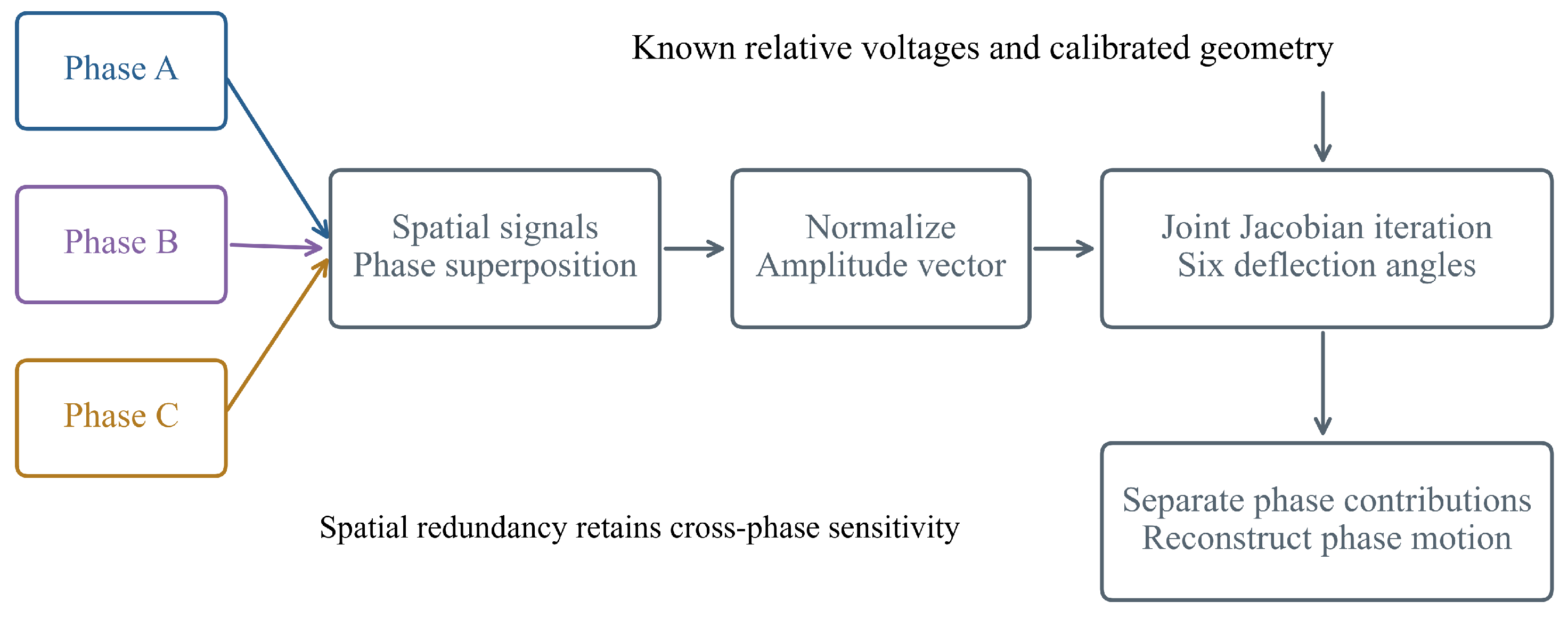
2.3. Three-Phase Electric-Field Separation and Joint Angle Reconstruction

Three-phase near-field contributions superpose at the measurement nodes. Let each phase have angles ${\alpha }_p,{\beta }_p$, and let column ${\mathbf{g}}_p$ of $\mathbf{G}$ be its gain-corrected unit-voltage probe response, including geometry and the adopted grounded boundary. Define

$$\theta ={[{\alpha }_A,{\beta }_A,{\alpha }_B,{\beta }_B,{\alpha }_C,{\beta }_C]}^T,\mathbf{b}\left(\theta \right)=\mathbf{G}\left(\theta \right)\eta ,h_i=\left|b_i\right|.$$

(29)

Here ${\eta }_p={\rho }_p\exp \left(j{\psi }_p\right)$ specifies known relative voltage magnitudes and phases. Balanced voltages use unit relative magnitudes and phase offsets $0,-2\pi /3,2\pi /3$; known unbalanced voltages use their corresponding values. For the gain-corrected amplitude vector $\mathbf{a}$ from N synchronous channels, define

$$\mathbf{y}={\displaystyle \frac{\mathbf{a}}{{\parallel \mathbf{a}\parallel }_2}},\mathbf{F}\left(\theta \right)={\displaystyle \frac{\mathbf{h}\left(\theta \right)}{{\parallel \mathbf{h}\left(\theta \right)\parallel }_2}}.$$

(30)

Normalization removes the common amplitude scale and retains spatial differences caused by phase superposition. All cross-phase sensitivities are included. Local updates are

$${\mathbf{J}}_k={\left.{\displaystyle \frac{\partial \mathbf{F}}{\partial \theta }}\right|}_{{\theta }_k},{\delta }_k={({\mathbf{J}}_k^T{\mathbf{J}}_k+{\lambda }_k\mathbf{I})}^{-1}{\mathbf{J}}_k^T[\mathbf{y}-\mathbf{F}\left({\theta }_k\right)],{\theta }_{k+1}={\theta }_k+{\delta }_k.$$

(31)

At least seven channels are needed to supply six independent normalized-amplitude constraints; this count does not itself guarantee $rank\left({\mathbf{J}}_k\right)=6$. A nine-node arrangement is a candidate spatial observation scheme. Work in a differentiable region with nonzero total amplitude and check rank and the smallest singular value for the specified geometry. After convergence, let $\widehat{\mathbf{h}}=\mathbf{h}\left(\widehat{\theta }\right)$ and recover phase contributions as

$$\widehat{c}={\displaystyle \frac{{\widehat{\mathbf{h}}}^T\mathbf{a}}{{\widehat{\mathbf{h}}}^T\widehat{\mathbf{h}}}},{\widehat{\mathbf{u}}}_p=\widehat{c}{\eta }_p{\mathbf{g}}_p\left({\widehat{\theta }}_p\right)=\widehat{c}\mathbf{b}\left(\widehat{\theta }\right)-\sum _{q\ne p}{\widehat{\mathbf{u}}}_q.$$

(32)

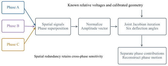
The recovered phase angles enter the same single-conductor geometry. This is a theoretical multiphase extension; the laboratory measurements assess the single-conductor sensing and inversion stage. Figure 2 summarizes the observation and reconstruction procedure.

Figure 2. Three-phase observation, joint six-angle recovery and phase-contribution separation.

3. Acquisition and Identification of Galloping Characteristics

3.1. Galloping Frequency Identification

The local inversion in Section 2.2 yields discrete-time tangent-angle sequences. Under a prescribed spatial mode with nonzero suspension-point slope sensitivity, its temporal motion modulates these sequences. Spectral analysis therefore extracts dominant periodic components within the monitoring search interval. The experimental spectra and known-input numerical frequency errors are reported separately in Section 4.3.

Taking the vertical direction as an example, assuming that the sensor array performs sampling at a constant sampling rate $f_s$ with a sampling time interval of $\mathsf{\Delta }t=1/f_s$, the galloping amplitude $A_y\left(k\mathsf{\Delta }t\right)$ obtained within a single sampling period is, in physical essence, a transient manifestation of the maximum galloping amplitude $A_{y\max }$ evolving over time. It satisfies the following time-domain mapping equation:

$$A_y\left(k\mathsf{\Delta }t\right)=A_{y\max }\sin (2\pi f_{y}k\mathsf{\Delta }t+{\phi }_y)$$

(33)

where $A_{y\max }$ represents the maximum galloping amplitude that the conductor can excite under the current aerodynamic load; $f_y$ denotes the dominant frequency of the vertical galloping; and ${\phi }_y$ is the initial phase.

During the continuous online monitoring process, according to the established solution mechanism, a series of discrete transient antinode amplitude sequences with equal time intervals can be generated as $A_y=[A_y\left(\mathsf{\Delta }t\right),A_y\left(2\mathsf{\Delta }t\right),\cdots ,A_y\left(N\mathsf{\Delta }t\right)]$. Subsequently, this time-domain discrete sequence is mapped into the frequency-domain space via an orthogonal transformation:

$$F_y\left(\omega \right)=\mathcal{F}\left\{A_y\right\}$$

(34)

Here $\mathcal{F}$ denotes the Fourier transform and $\omega$ angular frequency. A peak search in the magnitude spectrum estimates dominant temporal frequencies without first estimating the phase. Finite-record leakage, windowing and observation noise still affect peak location and amplitude. The effective sequence sampling rate, record length, window and interpolation procedure are specified for the numerical validation rather than inferred from the raw carrier sampling rate.

3.2. Galloping Order Identification

After acquiring the actual dominant galloping frequency, it is necessary to deduce the galloping order with the aid of the intrinsic characteristics of the conductor. As the core parameters determining the multi-order standing wave profiles, the transient galloping orders of the conductor in three-dimensional space (i.e., the vertical order $n_y$ and the horizontal order $n_x$) are prerequisites for the joint solution of the galloping amplitudes.

Under the combined effects of ice accretion and wind loads, overhead conductors actually exhibit extremely complex multi-modal coupled vibrations. However, the vast majority of the energy that causes structural damage and electrical accidents on transmission lines is concentrated in low-frequency, large-amplitude, low-order modes (typically orders 1 to 3). Therefore, this method treats multi-order minute high-frequency disturbances and non-steady-state onset processes as background noise during frequency-domain processing.

With small bending stiffness, an ideal taut string provides a reference frequency for tension-controlled small out-of-plane vibration, using horizontal tension and mass per unit length. A model retaining catenary geometry and spatially varying static tension was compared under equal-height fixed supports and linear small vibration. The calculated discrepancies for the specified sag-to-span range are summarized below.

$$f_1={\displaystyle \frac{1}{2L}}\sqrt{{\displaystyle \frac{T}{m}}}$$

(35)

Here T is the horizontal tension component, and m is the mass per unit length. The comparison in Table 3 quantifies the specified out-of-plane approximation. Spatial-order estimation uses correspondence between temporal frequency and spatial modes. For approximately harmonic out-of-plane modes, the reference-frequency ratio is rounded, with frequency uncertainty considered near half-integer boundaries. Prescribed-input validation treats spatial orders as known inputs, whereas manual-traction spectra describe imposed temporal motion.

$$\left\{\begin{array}{cc}\hfill n_y& =\mathrm{round}\left({\displaystyle \frac{f_{ymean}}{f_1}}\right)\hfill \\ \hfill n_x& =\mathrm{round}\left({\displaystyle \frac{f_{xmean}}{f_1}}\right)\hfill \end{array}\right.$$

(36)

where $\mathrm{round}\left(\right)$ represents the round-to-nearest-integer operator. Thus, the identification of the unknown discrete modal orders $n_x$ and $n_y$ is completed.

Table 3. Ideal-string and catenary-cable frequencies at selected sag ratios.

Sag Ratio (%)	Mode	String (Hz)	Cable (Hz)	Absolute $\mathsf{\Delta }$f (Hz)	Relative Error (%)
2.000	1	2.260995	2.260523	0.000472	0.02089
2.000	2	4.521990	4.519947	0.002042	0.04518
2.000	3	6.782985	6.779617	0.003368	0.04968
3.333	1	1.752186	1.751172	0.001015	0.05794
3.333	2	3.504372	3.499987	0.004386	0.12530
3.333	3	5.256558	5.249329	0.007229	0.13772
4.000	1	1.600037	1.598705	0.001332	0.08333
4.000	2	3.200074	3.194317	0.005757	0.18023
4.000	3	4.800112	4.790623	0.009488	0.19806

Both models use a 3 m span, mass per unit length 0.01 kg/m and the same horizontal tension at each sag. Relative error uses the cable frequency as reference. The underlying comparison uses 32 sine basis functions and 2001 integration points, checked with 64 functions and 4001 points. These are deterministic out-of-plane modal calculations.

3.3. Galloping Amplitude Calculation

According to the geometric interpretation of calculus, the tangential angle at the conductor suspension point ($z=0$) is equivalent to the first-order partial derivative of the transient spatial equations at that location. Differentiating the dynamic spatial system of equations in Equation (2) with respect to z at $z=0$ yields the analytical mapping between the root tangential slope and the morphological parameters:

$$\left\{\begin{array}{cc}\hfill k_x& =\tan \beta ={\left.{\displaystyle \frac{\partial X(z,t)}{\partial z}}\right|}_{z=0}=A_x{\displaystyle \frac{n_x\pi }{L}}\hfill \\ \hfill k_y& =\tan \alpha /\cos \beta ={\left.{\displaystyle \frac{\partial Y(z,t)}{\partial z}}\right|}_{z=0}=A_y{\displaystyle \frac{n_y\pi }{L}}-{\displaystyle \frac{4f_{sag}\left(t\right)}{L}}\hfill \end{array}\right.$$

(37)

Equation (37) reveals the inherent characteristics of the electric-field inversion: For the horizontal direction, the horizontal amplitude $A_x$ can be directly and linearly resolved from the horizontal deflection angle $\beta$. However, for the vertical direction, the measured vertical elevation angle $\alpha$ is actually a coupled result of the linear superposition of the transient vertical amplitude $A_y\left(t\right)$ and the transient dynamic sag $f_{sag}\left(t\right)$. There exist infinitely many combinations of $(A_y,f_{sag})$ that can produce the exact same suspension-point elevation angle $\alpha$. Without additional physical constraints, conventional inversion algorithms will inevitably yield multiple solutions.

To resolve this multi-solution issue, the arc-length conservation equation, Equation (6) from Section 2.1, is introduced. The arc length $S_0$, serving as an inherent rigid geometric boundary of the system, provides a crucial supplementary condition for the underdetermined system of equations.

From the vertical slope equation, the unknown amplitude $A_y\left(t\right)$ can be expressed as a function of $f_{sag}\left(t\right)$:

$$A_y\left(t\right)={\displaystyle \frac{L\tan \alpha /\cos \beta +4f_{sag}\left(t\right)}{n_y\pi }}$$

(38)

Substituting the decoupled $A_x$ and the above expression for $A_y\left(t\right)$ simultaneously into the arc-length conservation polynomial yields:

$$\begin{array}{cc}\hfill \mathsf{\Delta }S=& {\displaystyle \frac{8f_{sag}^2}{3L}}+{\displaystyle \frac{L}{4}}{\left({\displaystyle \frac{\tan \alpha }{\cos \beta }}+{\displaystyle \frac{4f_{sag}}{L}}\right)}^2+{\displaystyle \frac{L}{4}}{\tan }^2\beta \hfill \\ \hfill & -{\displaystyle \frac{8c_n{f}_{sag}}{n_y^2{\pi }^{2}L}}\left({\displaystyle \frac{L\tan \alpha }{\cos \beta }}+4f_{sag}\right),c_n=1-{(-1)}^{n_y}.\hfill \end{array}$$

(39)

Letting the known physical arc-length constant be $\mathsf{\Delta }S=S_0-L$, expanding the above equation and collecting like terms simplifies the system into a standard quadratic equation in one variable solely concerning the transient dynamic sag $f_{sag}\left(t\right)$:

$$\left({\displaystyle \frac{20}{3L}}-{\displaystyle \frac{32c_n}{n_y^2{\pi }^{2}L}}\right)f_{sag}^2+\left(2-{\displaystyle \frac{8c_n}{n_y^2{\pi }^2}}\right){\displaystyle \frac{\tan \alpha }{\cos \beta }}{f}_{sag}+{\displaystyle \frac{L}{4}}\left({\displaystyle \frac{{\tan }^2\alpha }{{\cos }^2\beta }}+{\tan }^2\beta \right)-\mathsf{\Delta }S=0.$$

(40)

Under the inextensibility assumption, the total conductor arc length must be conserved during reconstruction. Select a feasible sag branch continuous with the static state and check the residual of the full arc-length integral. Positivity alone does not guarantee a unique physically admissible branch. The reconstructed midspan displacements relative to the static profile are $A_y\sin (n_y\pi /2)-f_{sag}+f_0$ and $A_x\sin (n_x\pi /2)$. The vertical displacement therefore includes sag variation.

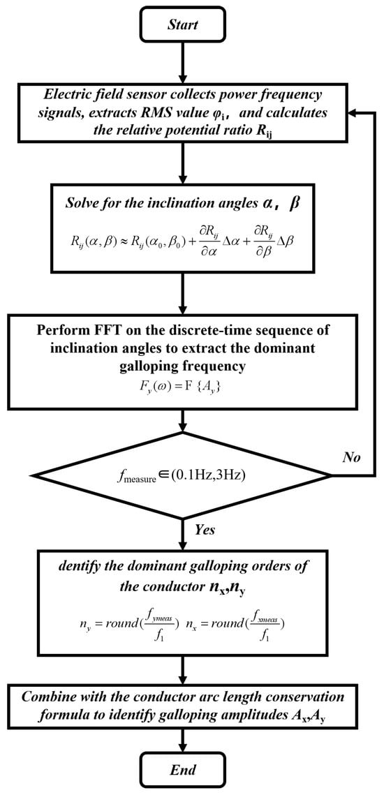
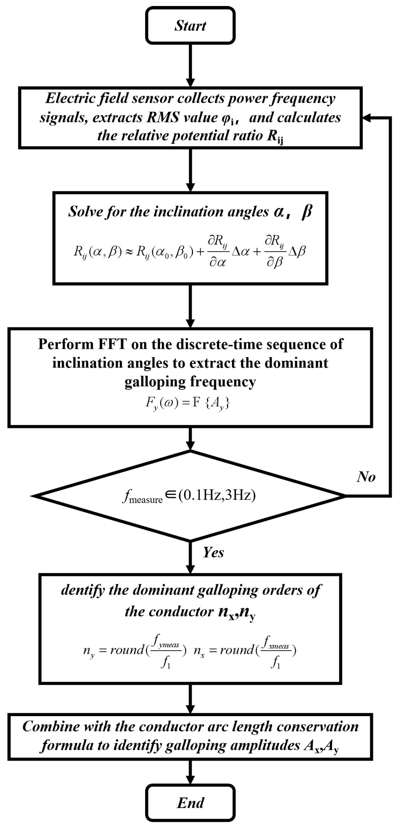
To this point, this method decomposes the complex nonlinearly coupled inversion problem into a two-step procedure: first, decoupling in the spatial domain by utilizing the electric-field boundary and arc-length conservation, and subsequently, extracting key parameters in the time domain via the time-series amplitude-frequency characteristics. This completely establishes the algebraic analytical and extraction method for the core parameters of conductor galloping (amplitude and frequency). The complete flowchart of this method is illustrated in Figure 3.

Figure 3. Flowchart of galloping characteristics detection method.

4. Experimental Results and Numerical Validation

4.1. Experimental Environment and Test Platform Setup

To assess the motion-sensing and inversion stages of the proposed galloping detection method, a laboratory platform was built for controlled conductor movement. The vertical and horizontal motions were applied separately to evaluate reconstruction of the corresponding displacement and temporal characteristics. The laboratory scene was arranged at a nominal geometric scale of 1:20, with a 3 m test span corresponding to a 60 m reference span. The initial sag of the test conductor was 0.10 m, giving a sag-to-span ratio of approximately 0.0333. A three-phase voltage regulator supplied one test conductor at a nominal 220 V and 50 Hz to establish a power-frequency electric field; a DC supply powered the sensor array, signal-conditioning circuits, and data-acquisition unit. The 1:20 designation defines the nominal geometric span scale.

The single-conductor laboratory experiment evaluates the target-phase measurement and inversion stage; the multiphase extension is developed in Section 2.3.

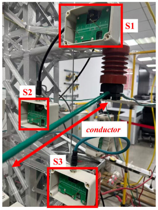
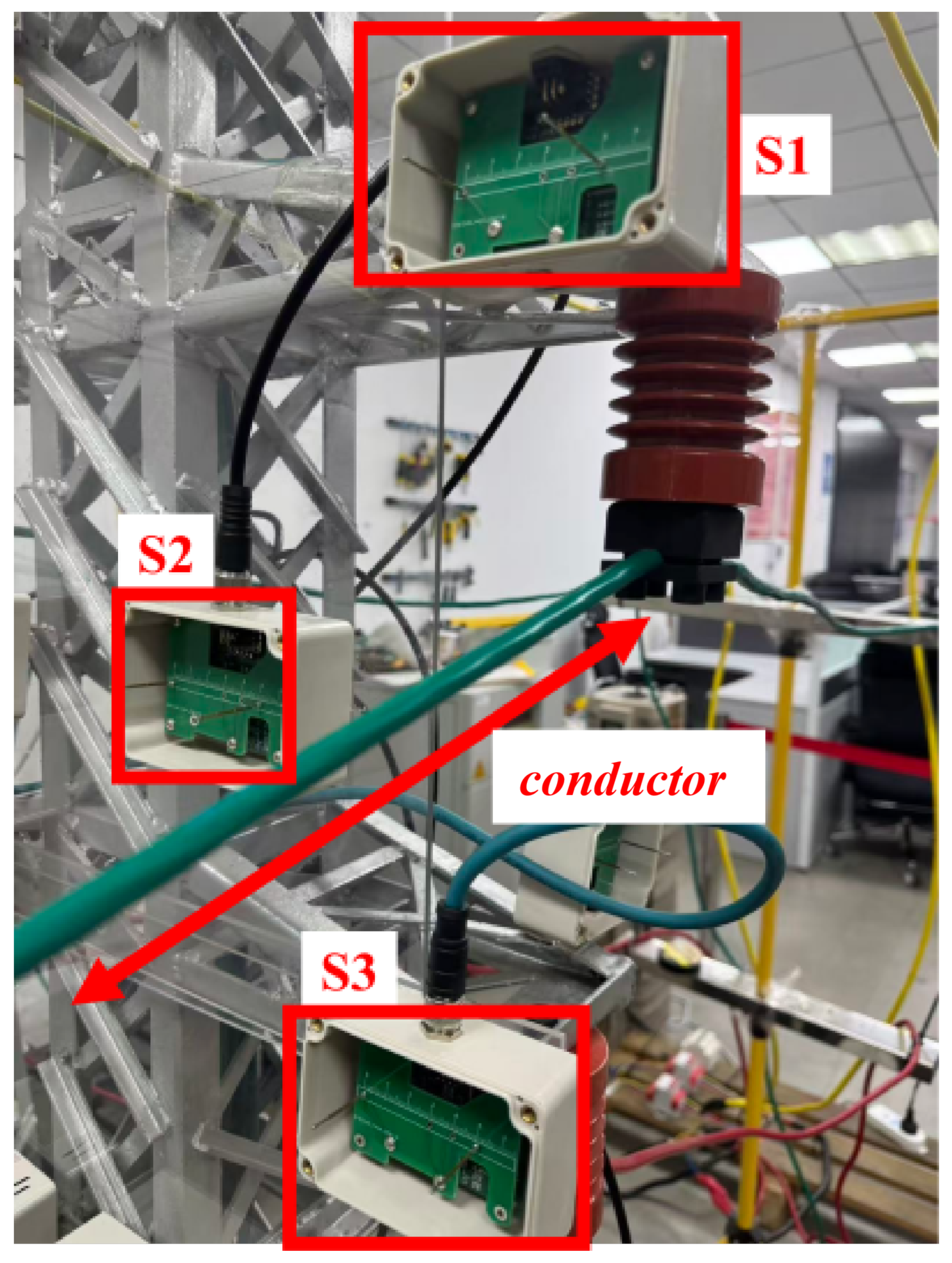
Regarding the deployment of the non-contact electric-field sensing, this paper adopted a non-collinear distributed sensor array composed of three independent electric-field sensors (designated as S1, S2, and S3), as shown in Figure 4.

Figure 4. Arrangement of sensors and test conductor.

A triangular spatial arrangement supplies multiple observations of the two angles, but non-collinearity alone does not guarantee full column rank. Array evaluation uses the sensitivities in Equations (20)–(25) to check rank and the smallest singular value throughout the working region. Position and orientation errors are propagated through the actual probe response. Let ${\mathbf{K}}_p,{\mathbf{K}}_{\omega }$ be the corresponding ratio derivatives and ${\mathsf{\Sigma }}_R$ the ratio-noise covariance, including the shared-reference correlation. For mutually uncorrelated zero-mean observation and installation perturbations,

$${\mathsf{\Sigma }}_{eff}={\mathsf{\Sigma }}_R+{\mathbf{K}}_p{\mathsf{\Sigma }}_p{\mathbf{K}}_p^T+{\mathbf{K}}_{\omega }{\mathsf{\Sigma }}_{\omega }{\mathbf{K}}_{\omega }^T,{\mathbf{C}}_{\mathsf{\Theta }}={\left({\mathbf{J}}^T{\mathsf{\Sigma }}_{eff}^{-1}\mathbf{J}\right)}^{-1}.$$

(41)

This covariance uses optimally weighted local estimation; an unweighted estimator uses its own general covariance propagation. With layout S and working region $\mathsf{\Omega }$, a placement criterion is

$$S^{\ast }=\arg \underset{S\in D_s}{\min }\underset{\mathsf{\Theta }\in \mathsf{\Omega }}{\max }{\lambda }_{max}\left[{\mathbf{C}}_{\mathsf{\Theta }}(\mathsf{\Theta },S)\right],\left|{\Phi }_1\right|\ge {\Phi }_{min},{\sigma }_{min}\left({\mathsf{\Sigma }}_{eff}^{-1/2}\mathbf{J}\right)\ge s_{min}.$$

(42)

The feasible domain $D_s$ enforces installation and safety distances, and the thresholds are design inputs. At fixed total information, balanced orthogonal whitened sensitivity columns minimize worst-direction variance. This criterion guides comparisons of candidate configurations; the laboratory arrangement is the existing array adjacent to the test conductor.

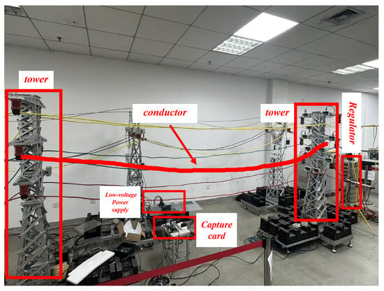
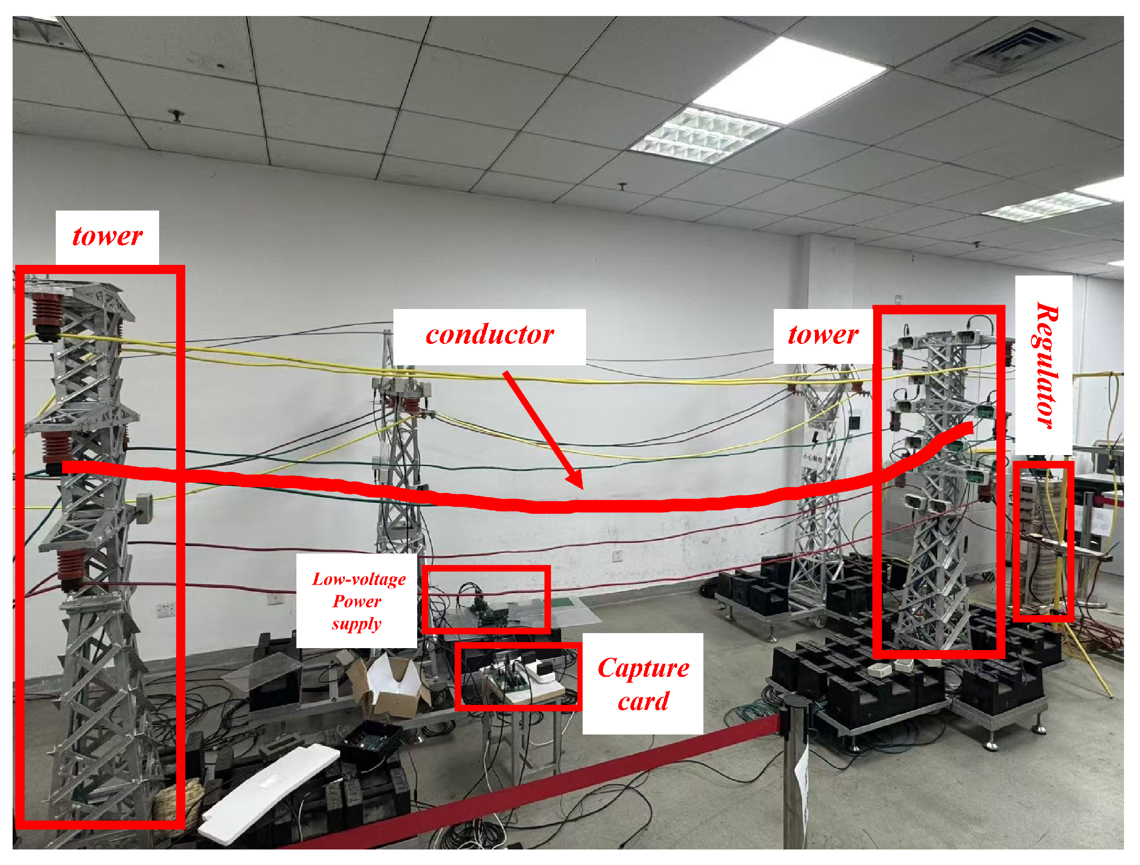
Figure 5 shows the laboratory platform used for the controlled conductor-motion tests.

Figure 5. Nominally 1:20 geometric-scale laboratory platform.

4.2. Spatial Electric-Field Sensor Design and Performance Testing

4.2.1. Device Design

The non-contact spatial electric-field sensing unit utilized in the experiments of this paper mainly consists of two core components: the electric-field sensing module and the signal processing module. Figure 6a shows the sensor assembly and hardware overview, while Figure 6b shows the on-board component interconnections and the separate reference connections.

(1) Electric-Field Sensing Module

The electric-field sensing module uses a pair of small parallel metal probes separated by approximately 5 cm. Sensors are fixed near the conductor as shown in the apparatus photograph. In laboratory testing the conductor is energized at a nominal 220 V and 50 Hz. Its movement changes the field over the probes and their coupling to the conductor, changing the two induced voltages. Probe geometry, installation geometry, and capacitive coupling to ground and supporting structures jointly determine spatial response. The probes connect to V+ and V- through separate 10 $\mu$F AC-coupling capacitors to the INA821IDR. Each amplifier-side input connects through 10 M$\mathsf{\Omega }$ to board GND for bias-current return. The front end reads the induced-voltage difference; shared-interference rejection depends on matching of the coupling and circuitry. Probe response and the channel transfer relation convert the field model into measurement voltage.

(2) Signal Processing Module

The INA821IDR preamplifier has a nominal gain of approximately 10 for its 5.49 k$\mathsf{\Omega }$ gain-setting resistor. Two OPA2388IDR sections form cascaded multiple-feedback bandpass stages followed by the PGA112AIDGSR. Nominal components and an ideal-op-amp model give a combined -3 dB passband of approximately 44.83 to 53.75 Hz and a magnitude gain of 3.89 at 50 Hz. PGA VREF and the second filter stage share the DC operating-point reference. The GD32F450ZIT6 ADC uses the separate REF_2.5V reference and a raw sampling rate of 10 kHz. Low-frequency conductor motion amplitude-modulates the carrier, producing sidebands around 50 Hz. Gain and phase at those sidebands, together with the digital averaging window and decimation settings, determine the amplitude and timing of the motion sequence. Inversion therefore uses carrier-amplitude observations corresponding to the field model, distinguishing DC offset, channel gain, and dynamic transfer response.

Figure 6. Hardware arrangement and on-board component interconnections of the electric-field sensor. (a) Sensor assembly and hardware overview. (b) Board-level connections of the input coupling and bias-return network, INA821 preamplifier, two OPA2388 bandpass sections, PGA112 and GD32F450 ADC/MCU. Solid black arrows indicate the signal path; dashed blue arrows indicate separate DC reference connections. GND denotes board ground, connected to AGND through a ferrite bead. The nominal circuit parameters are listed in Table 4.

Figure 6. Hardware arrangement and on-board component interconnections of the electric-field sensor. (a) Sensor assembly and hardware overview. (b) Board-level connections of the input coupling and bias-return network, INA821 preamplifier, two OPA2388 bandpass sections, PGA112 and GD32F450 ADC/MCU. Solid black arrows indicate the signal path; dashed blue arrows indicate separate DC reference connections. GND denotes board ground, connected to AGND through a ferrite bead. The nominal circuit parameters are listed in Table 4.

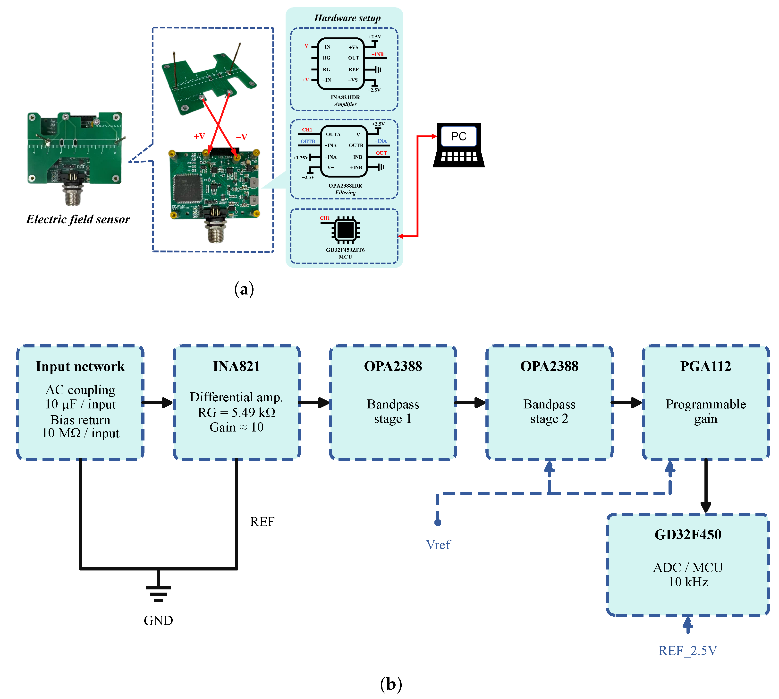
Detecting the weak electrode-induced signals requires a high-input-impedance front end and low-noise amplification. The amplified signal is bandpass-filtered around the carrier and digitized for subsequent envelope extraction. For matched branches, stable references and unsaturated amplifiers in the linear small-signal regime, the nominal analog chain is

$$H_{el}\left(s\right)={\displaystyle \frac{V_{out,ac}\left(s\right)}{\mathsf{\Delta }{V}_p\left(s\right)}}=H_{AC}\left(s\right)G_{INA}{H}_{BP1}\left(s\right)H_{BP2}\left(s\right)G_{PGA}.$$

(43)

The output DC operating level is removed before alternating amplitude extraction. Probe capacitance and loading determine $\mathsf{\Delta }{V}_p$; ADC acquisition and digital processing follow the analog chain.

Table 4. Nominal signal-chain components and references.

Stage	Parameter or Connection	Definition and Basis
Input AC coupling	10 $\mu$F per probe branch	Nominal component value; AC coupling.
Input bias return	10 M$\mathsf{\Omega }$ per input to GND	External bias-return resistance; the complete input impedance is determined jointly by the probes and front end.
INA821 preamplifier	RG = 5.49 k$\mathsf{\Omega }$; G ≈ 10	Nominal differential gain calculated as G = 1 + 49.4 k$\mathsf{\Omega }$/RG.
First OPA2388 bandpass stage	f0 ≈ 46.1 Hz; BW ≈ 6.24 Hz; peak gain ≈ 2.80	Analytical estimate for ideal op amps and nominal components; BW denotes −3 dB bandwidth.
Second OPA2388 bandpass stage	f0 ≈ 52.4 Hz; BW ≈ 7.40 Hz; peak gain ≈ 2.62	Calculated single-stage response under the same ideal-amplifier and nominal-component assumptions.
PGA112 selectable gain	1, 2, 4, 8, 16, 32	Settings listed in the schematic; operating gain is determined by the acquisition settings. The device also supports 64 and 128; these two settings are not annotated in the schematic.
Analog and digital supplies	INA821/OPA2388: ±2.5 V; PGA: analog 5 V, digital 3.3 V	Nominal supply-net values; the PGA analog supply is filtered.
Output-offset reference	Vref shared by OPA2388 stage 2 and PGA	Sets the electronic DC operating point; distinct from REF_2.5V.
ADC conversion reference	REF_2.5V: nominal 2.5 V	Separate ADC conversion-reference network.
Raw ADC sampling rate	10 kHz	Carrier sampling rate reported in the manuscript; the envelope-sequence rate is specified separately.
Board-level reference connection	GND connected to AGND through a ferrite bead	Board-reference and noise-control connection; site ground is connected through the sensor cable grounding conductor.
Combined bandpass response	Peak near 48.44 Hz; −3 dB passband 44.83–53.75 Hz; magnitude gain 3.89 at 50 Hz	Product of complex stage responses at the same frequency, calculated from nominal components and ideal amplifiers.

Table 4. Nominal signal-chain components and references.

Stage	Parameter or Connection	Definition and Basis
Input AC coupling	10 $\mu$F per probe branch	Nominal component value; AC coupling.
Input bias return	10 M$\mathsf{\Omega }$ per input to GND	External bias-return resistance; the complete input impedance is determined jointly by the probes and front end.
INA821 preamplifier	RG = 5.49 k$\mathsf{\Omega }$; G ≈ 10	Nominal differential gain calculated as G = 1 + 49.4 k$\mathsf{\Omega }$/RG.
First OPA2388 bandpass stage	f0 ≈ 46.1 Hz; BW ≈ 6.24 Hz; peak gain ≈ 2.80	Analytical estimate for ideal op amps and nominal components; BW denotes −3 dB bandwidth.
Second OPA2388 bandpass stage	f0 ≈ 52.4 Hz; BW ≈ 7.40 Hz; peak gain ≈ 2.62	Calculated single-stage response under the same ideal-amplifier and nominal-component assumptions.
PGA112 selectable gain	1, 2, 4, 8, 16, 32	Settings listed in the schematic; operating gain is determined by the acquisition settings. The device also supports 64 and 128; these two settings are not annotated in the schematic.
Analog and digital supplies	INA821/OPA2388: ±2.5 V; PGA: analog 5 V, digital 3.3 V	Nominal supply-net values; the PGA analog supply is filtered.
Output-offset reference	Vref shared by OPA2388 stage 2 and PGA	Sets the electronic DC operating point; distinct from REF_2.5V.
ADC conversion reference	REF_2.5V: nominal 2.5 V	Separate ADC conversion-reference network.
Raw ADC sampling rate	10 kHz	Carrier sampling rate reported in the manuscript; the envelope-sequence rate is specified separately.
Board-level reference connection	GND connected to AGND through a ferrite bead	Board-reference and noise-control connection; site ground is connected through the sensor cable grounding conductor.
Combined bandpass response	Peak near 48.44 Hz; −3 dB passband 44.83–53.75 Hz; magnitude gain 3.89 at 50 Hz	Product of complex stage responses at the same frequency, calculated from nominal components and ideal amplifiers.

4.2.2. Performance Testing

Before applying the sensor-array data to the galloping-related motion reconstruction, a preliminary laboratory test examined how the sensor output varied with conductor distance.

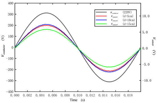
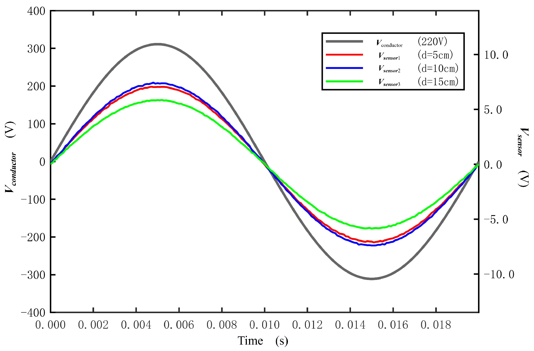
As can be seen from Equation (12), the potential generated by the conductor at a certain point in space is negatively correlated with the distance from that point to the conductor. As an initial check of distance sensitivity under the laboratory setup, the sensor output was recorded at conductor separations of 5 cm, 10 cm, and 15 cm. The resulting voltage waveforms are shown in Figure 7.

Figure 7. Variation of output voltage with distance.

Within the three tested separations, the sensor-output amplitude decreases as the distance increases, while the phase relationship shown in Figure 7 remains similar. This preliminary observation supports the use of the sensor for the subsequent laboratory motion tests; it does not by itself establish performance during actual conductor galloping.

4.3. Frequency Feature Extraction and Validation

4.3.1. Angle Reconstruction and Periodic Motion Features

The angle and displacement comparisons use the laboratory geometry with a 3 m span and a 0.10 m initial sag. The manual-traction spectra and the angle comparisons are separate records. The spectra characterize the periodic components of imposed laboratory motion, while the numerical references provide paired comparisons for the reconstruction calculation. The reported angles use the small-angle slope equivalents, ${\alpha }_{num}=k_{y}180/\pi$ and ${\beta }_{num}=k_{x}180/\pi$. The dynamic angle record and the quasi-static displacement record in Section 4.4 have different motion histories. The common laboratory geometry and processing settings are listed in Table 5.

Table 5. Laboratory geometry and processing settings for the angle and displacement comparisons.

Parameter	Setting
Laboratory span	3 m
Initial sag	0.10 m
Supply and coupling coefficient	220 V RMS, 50 Hz; 0.02
Sensor coordinates/m	(−0.5, −1.0, 0.04); (−0.3, −1.2, 0.04); (−0.5, −2.0, 0.04)
Motion sequence and ADC sampling	50 Hz; 10 kHz
Duration and smoothing	10 s; 8-frame centered moving average
Noise and seed	Measured-power AWGN SNR 45 dB; seed 20261012
Spatial orders	nx = ny = 1

The dynamic angle and quasi-static displacement records are distinct, but both use the stated 3 m laboratory span and 0.10 m initial sag. Numerical noise settings describe the assumed reference calculation, not measured hardware uncertainty.

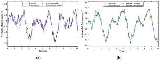
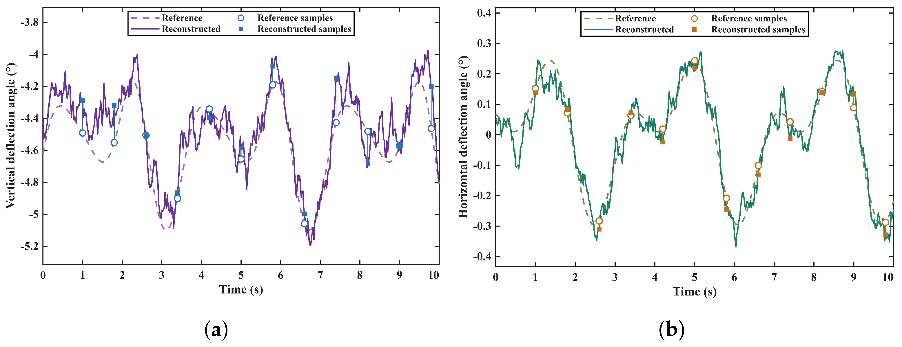
Figure 8 compares the reference and reconstructed vertical and horizontal small-angle slope equivalents.

Figure 8. Reference and recovered small-angle slope equivalents for the prescribed dynamic numerical record. (a) Vertical direction; (b) horizontal direction. Markers identify the twelve comparison times.

The angle waveforms preserve the main prescribed changes, with pointwise and full-record errors in Table 6, Table 7 and Table 8. Separately, an FFT was applied to the laboratory reconstructed inclination-angle sequences to describe their imposed periodic components. The raw carrier sampling rate differs from the effective motion-sequence sampling rate. Frequency errors against prescribed inputs are evaluated in Section 4.3.2.

Table 6. Twelve-point vertical numerical angle comparison.

Sampling Point	t/s	Reference/∘	Reconstructed/∘	Absolute Error/∘	Reference-Peak Normalized Error/%
1	1.0	−4.492	−4.290	0.203	3.98
2	1.8	−4.551	−4.320	0.231	4.53
3	2.6	−4.506	−4.509	0.003	0.06
4	3.4	−4.901	−4.865	0.035	0.69
5	4.2	−4.342	−4.399	0.057	1.12
6	5.0	−4.654	−4.585	0.069	1.35
7	5.8	−4.190	−4.074	0.116	2.28
8	6.6	−5.058	−4.997	0.061	1.21
9	7.4	−4.427	−4.150	0.277	5.44
10	8.2	−4.482	−4.684	0.202	3.96
11	9.0	−4.571	−4.570	0.000	0.00
12	9.8	−4.464	−4.202	0.262	5.13

Reference-peak normalization uses p = 5.097943 degrees; errors were calculated before rounding.

Table 7. Twelve-point horizontal numerical angle comparison.

Sampling Point	t/s	Reference/∘	Reconstructed/∘	Absolute Error/∘	Reference-Peak Normalized Error/%
1	1.0	0.152	0.138	0.014	4.83
2	1.8	0.072	0.083	0.011	3.80
3	2.6	−0.283	−0.310	0.027	9.21
4	3.4	0.064	0.072	0.009	2.89
5	4.2	0.019	−0.024	0.042	14.31
6	5.0	0.244	0.220	0.024	8.12
7	5.8	−0.208	−0.245	0.037	12.46
8	6.6	−0.101	−0.132	0.031	10.40
9	7.4	0.042	−0.012	0.055	18.42
10	8.2	0.142	0.139	0.003	1.04
11	9.0	0.089	0.133	0.044	14.94
12	9.8	−0.288	−0.329	0.041	13.72

Reference-peak normalization uses p = 0.296692 degrees; errors were calculated before rounding.

Table 8. Numerical angle-error statistics.

Direction and Scope	N	MAE	RMSE	MaxAE	MedAE	Bias	Range NRMSE/%
Vertical 12 points	12	0.1264	0.1600	0.2772	0.0925	0.0827	17.26
Horizontal 12 points	12	0.0282	0.0322	0.0547	0.0291	−0.0175	5.96
Vertical full trace	501	0.1078	0.1353	0.4906	0.0918	0.0706	14.61
Horizontal full trace	501	0.0331	0.0414	0.1275	0.0272	−0.0059	7.64

MAE, RMSE, MaxAE, MedAE and Bias are in degrees. Range NRMSE divides RMSE by the complete reference range. N counts time points within one record, not independent replicates.

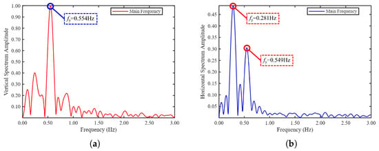
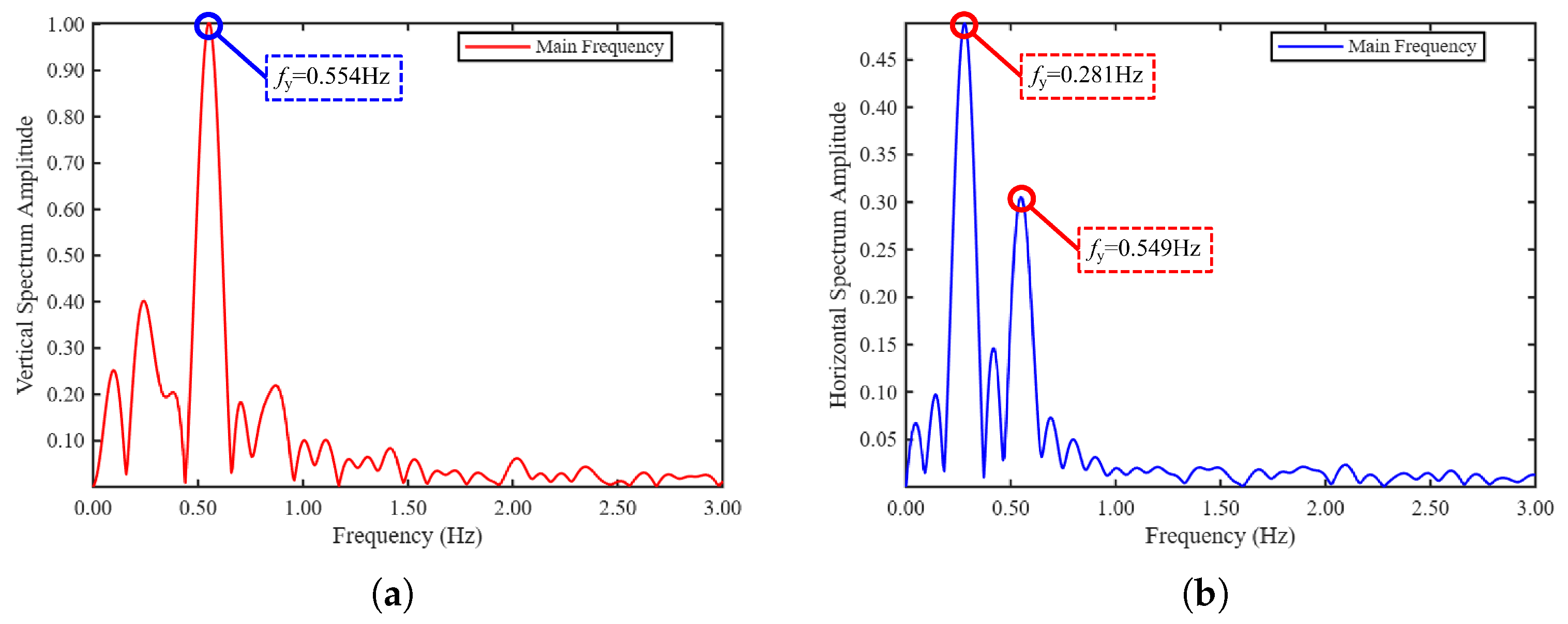
The dominant peaks at 0.555 Hz vertically and 0.281 Hz horizontally characterize periodic components in the separate manual-traction records. Frequency errors against known inputs are evaluated separately in Section 4.3.2.

Figure 9 shows the vertical and horizontal frequency spectra from the separate manual-traction records.

Figure 9. Frequency spectra of reconstructed conductor motion under manual traction. (a) Vertical direction. (b) Horizontal direction.

4.3.2. Known-Input Numerical Frequency Recovery

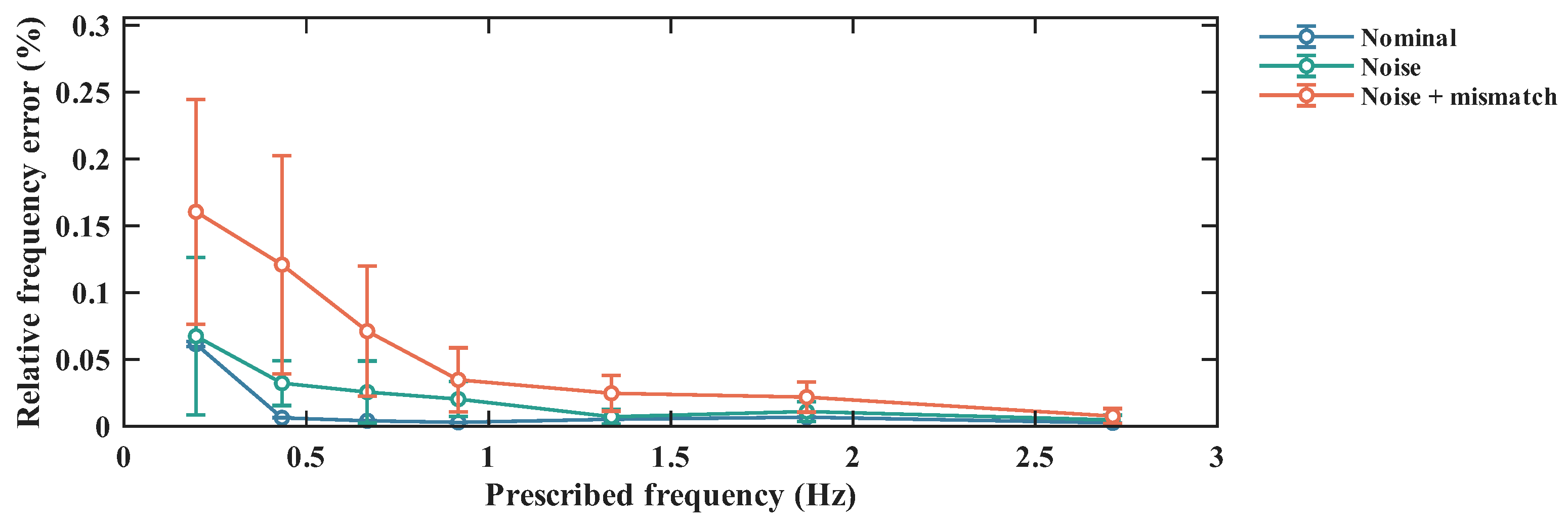
Known-input numerical tests were added to evaluate frequency recovery separately from the manual-traction observations. The forward model generates differential voltages for finite-area probe pairs with an approximately 50 mm separation, a 50 Hz modulated carrier, circuit conditioning and ADC quantization. The inverse uses nominal channel-gain correction and a static Jacobian of differential-voltage ratios. This is a dual-probe extension of the local ratio-inversion formulation, rather than a direct substitution of point potentials for measured voltages. Vertical and horizontal motion are prescribed simultaneously as

$$q_d\left(t\right)=A_d\left[\sin (2\pi f_{d}t+{\varphi }_d)+h_d\sin (4\pi f_{d}t+0.7)\right],d\in \{v,h\}.$$

(44)

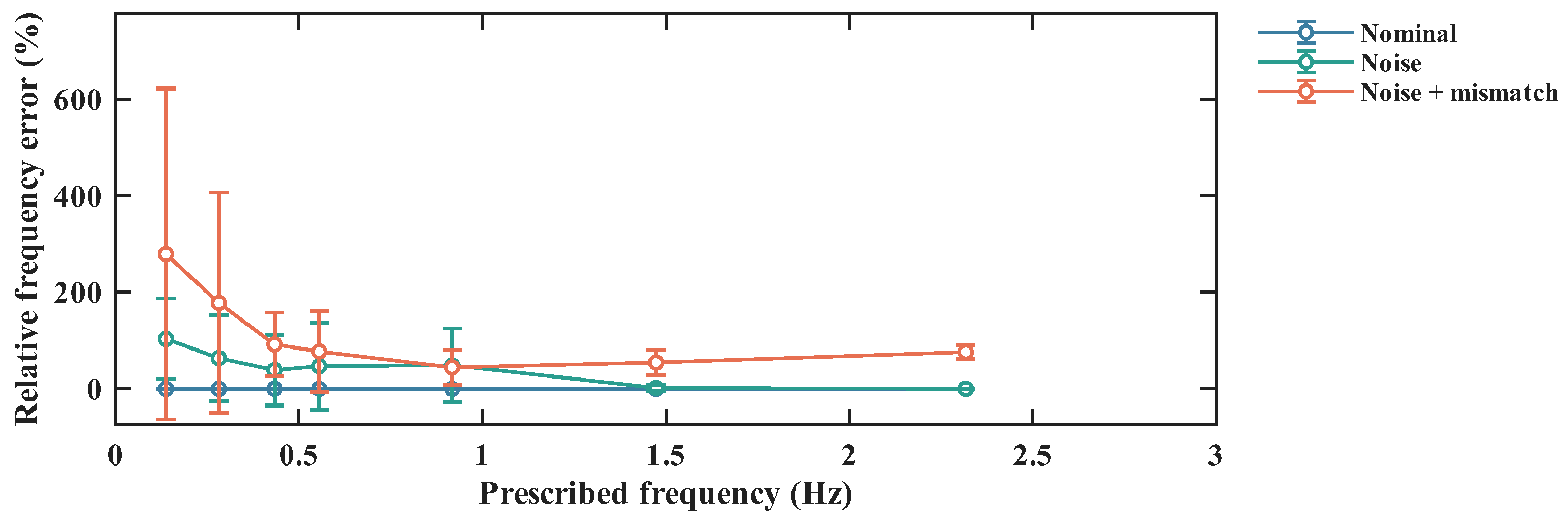
Vertical and horizontal fundamental amplitudes are 2.0 and 1.8 cm, with second-harmonic fractions of 0.08 and 0.06. The vertical input frequencies are 0.137, 0.281, 0.433, 0.555, 0.917, 1.473 and 2.317 Hz; corresponding horizontal frequencies are 0.197, 0.433, 0.667, 0.917, 1.337, 1.873 and 2.713 Hz. Each pair is evaluated through 12 random-phase runs under nominal, noise and noise-plus-mismatch conditions. These are numerical repetitions. The prescribed frequency and displacement are withheld from inversion and peak estimation.

The carrier is sampled at 10 kHz with assumed 12-bit quantization. Non-overlapping whole-cycle synchronous I/Q integration produces amplitude sequences at 50 Hz. Reconstructed displacement is analyzed over 120 s using linear detrending, a symmetric Hann window and a 6000-point FFT without zero-padding. The original bin spacing is 0.00833 Hz. A fixed 0.1–3 Hz search interval and three-point log-amplitude parabolic interpolation are used for all runs. The noise scenario assumes an ADC voltage-noise standard deviation of 4 mV and coupling-amplitude jitter of 0.5%; the combined scenario uses 8 mV and 1.5%, together with geometry and component deviations. These assumed disturbances are sensitivity-test settings, not measured device uncertainties. Frequency errors are evaluated against the prescribed input as

$${\epsilon }_{d,r}=100{\displaystyle \frac{|{\widehat{f}}_{d,r}-f_{d,r}|}{f_{d,r}}}\%,{\mathrm{RMSE}}_{f,d}=\sqrt{{\displaystyle \frac{1}{M}}\sum _{r=1}^M{({\widehat{f}}_{d,r}-f_{d,r})}^2}.$$

(45)

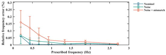
Figure 10 and Figure 11 report mean absolute relative error and sample standard deviation at each prescribed frequency. Pooled errors and processing settings are given in Table 9 and Table 10. Horizontal recovery remains comparatively stable under the prescribed perturbations, whereas vertical estimates show substantial misidentification. Original bin spacing, estimated frequency error and physical calibration uncertainty are distinct quantities.

Figure 10. Vertical frequency-recovery errors in known-input numerical tests under nominal, noise and noise-plus-mismatch conditions. Markers show mean absolute relative error; error bars show sample standard deviation over 12 numerical runs per frequency.

Figure 11. Horizontal frequency-recovery errors in known-input numerical tests. Scenarios and statistical definitions match Figure 10; directions are reported separately.

Table 9. Known-input frequency-validation processing settings.

Parameter	Numerical Setting
Data and reference	Model-generated two-direction inputs; reference withheld from estimator
Carrier and raw sampling	50 Hz; ADC 10 kHz; 12-bit quantization assumed
Demodulation and effective rate	Non-overlapping one-cycle rectangular I/Q integration; output 50 Hz
Window and samples	120 s; 6000 samples; FFT 6000 points; no zero-padding
Preprocessing and window	Linear detrending; symmetric Hann window
Peak search and interpolation	Fixed 0.1–3 Hz; three-point log-amplitude parabola
Repetitions	12 random-phase/noise numerical runs per frequency and scenario
Inversion and statistics	Static differential-voltage-ratio Jacobian; mean ± sample SD

Table 10. Frequency-recovery errors across seven prescribed frequencies.

Scenario	Direction	RMSE (Hz)	Max. Relative Error (%)	Over One Bin (n/84)
Nominal	Vertical	9.32989 × 10−5	0.136	0/84
Nominal	Horizontal	7.8399 × 10−5	0.064	0/84
Noise	Vertical	0.414682	230.636	25/84
Noise	Horizontal	0.000190406	0.185	0/84
Noise + mismatch	Vertical	0.914214	1157.552	81/84
Noise + mismatch	Horizontal	0.000446183	0.311	0/84

Pooled RMSE uses 84 estimates per direction and scenario. Error bars use 12 numerical runs at each prescribed frequency; these do not constitute physical repeatability measurements.

4.4. Displacement Reconstruction and Error Evaluation

4.4.1. Laboratory Scale-Reference Comparisons

To examine the displacement-reconstruction stage of the galloping detection method, manual traction was applied separately in the horizontal and vertical directions to generate low-frequency motion of the energized conductor. During traction, the displacement of the conductor at midspan was recorded using a scale and used as the experimental reference. The sensor-array signals were processed to estimate the corresponding midspan displacement. The test lasted 10 s, and six selected times were used for the error comparison. The scale readings provide a displacement reference, with uncertainty contributions from scale resolution, manual reading, and temporal alignment with the sensor signals. The comparison evaluates the sensing-to-displacement reconstruction chain at the selected times.

Table 11 and Table 12 present the vertical and horizontal displacement comparisons at the six selected laboratory times, respectively.

Table 11. Six selected laboratory displacement comparisons in the vertical direction.

Point	Time/s	Reference/m	Reconstructed/m	Absolute Error/m
1	1.0	0.767	0.919	0.152
2	2.6	0.113	0.027	0.086
3	4.2	−0.539	−0.550	0.011
4	5.8	0.233	0.176	0.057
5	7.4	0.232	0.199	0.033
6	9.0	−0.419	−0.344	0.075

These scale-reference pairs are laboratory data; they are distinct from the twelve-point numerical comparison below.

Table 12. Six selected laboratory displacement comparisons in the horizontal direction.

Point	Time/s	Reference/m	Reconstructed/m	Absolute Error/m
1	1.0	−0.436	−0.391	0.045
2	2.6	0.027	0.014	0.013
3	4.2	0.440	0.432	0.008
4	5.8	−0.093	−0.158	0.065
5	7.4	−0.127	−0.089	0.038
6	9.0	0.273	0.231	0.042

These scale-reference pairs are laboratory data; they are distinct from the twelve-point numerical comparison below.

The scale-reference comparison evaluates the sensing-to-displacement chain at the selected laboratory times; its error statistics are given in Table 13. The numerical comparison below supplies complete simulated-reference sequences for denser error reporting, separately from the experimental samples.

Table 13. Error statistics calculated from the six laboratory reference pairs.

Direction	N	MAE	RMSE	MaxAE	MedAE	Bias	NRMSE/%
Vertical	6	0.0690	0.0822	0.1520	0.0660	0.0067	6.30
Horizontal	6	0.0352	0.0402	0.0650	0.0400	−0.0075	4.59

Absolute metrics are in meters. N counts paired comparison times within one laboratory record. Range NRMSE uses the observed reference ranges of 1.306 m vertically and 0.876 m horizontally. Calculations use the rounded reference and reconstruction values in the original experimental tables.

4.4.2. Known-Input Numerical Displacement Comparisons

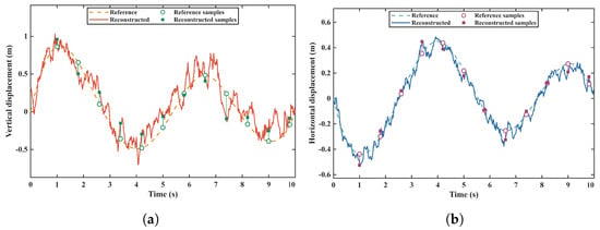
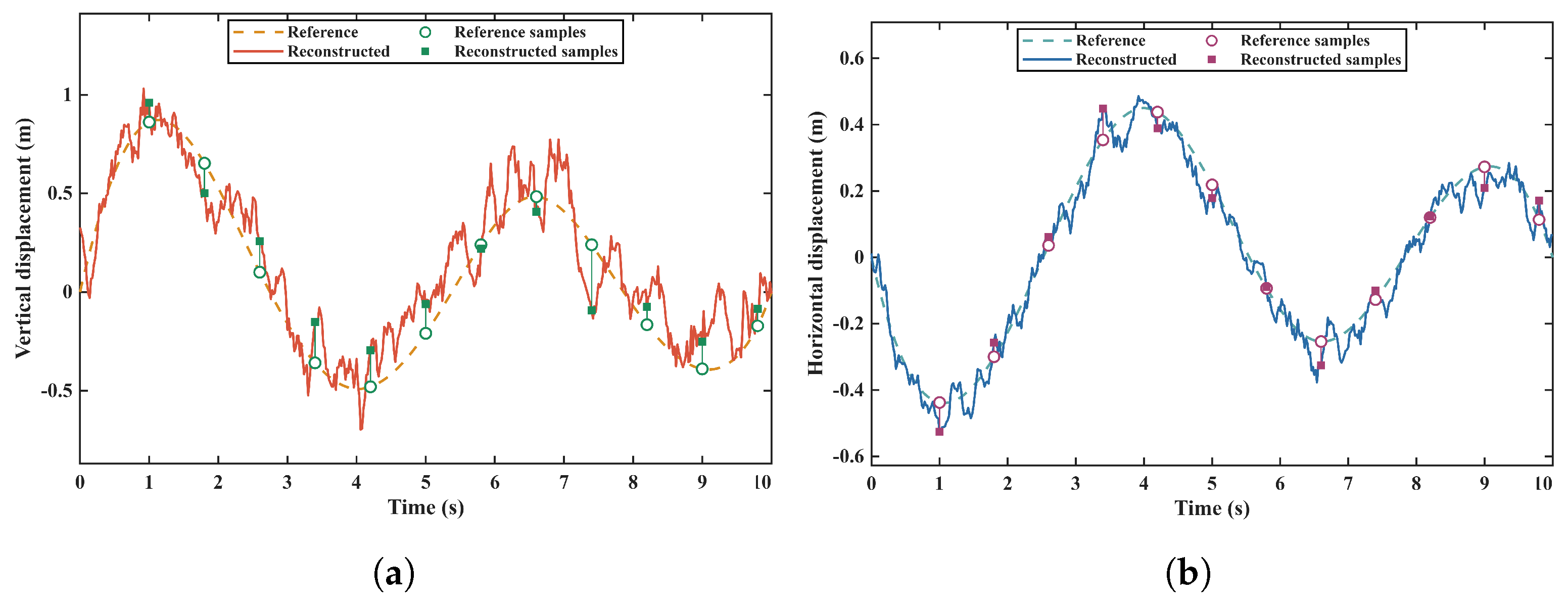
The displacement comparison uses the 3 m laboratory span and 0.10 m initial sag listed in Table 5, separately from the dynamic angle record. Vertical midspan displacement is $A_y-f+f_0$, and horizontal displacement is $A_x$. Figure 12 shows the paired waveforms. The same twelve preset times are used for pointwise evaluation in both directions.

Figure 12. Reference and reconstructed midspan displacement in the supplied quasi-static numerical record. (a) Vertical direction; (b) horizontal direction. Markers show twelve preset comparison times.

For reference $x_{ref,i}$ and reconstruction ${\widehat{x}}_i$, define $e_i={\widehat{x}}_i-x_{ref,i}$, $A{E}_i=\left|e_i\right|$, $P={\max }_t\left|x_{ref}\left(t\right)\right|$ and $R={\max }_t{x}_{ref}\left(t\right)-{\min }_t{x}_{ref}\left(t\right)$. Pointwise normalized error is $100A{E}_i/P$; range-normalized RMSE is $100RMSE/R$. The denominators are reference-waveform scales, not instrument full-scale values. MAE, RMSE, maximum absolute error, median absolute error and bias are computed from the same paired samples.

Table 14 and Table 15 list the twelve-point vertical and horizontal displacement comparisons, respectively; Table 16 summarizes the pointwise and complete-record errors.

Table 14. Twelve-point vertical numerical displacement comparison.

Sampling Point	t/s	Reference/m	Reconstructed/m	Absolute Error/m	Reference-Peak Normalized Error/%
1	1.0	0.862	0.960	0.098	11.26
2	1.8	0.652	0.501	0.151	17.32
3	2.6	0.101	0.257	0.156	17.94
4	3.4	−0.359	−0.151	0.208	23.87
5	4.2	−0.480	−0.295	0.185	21.20
6	5.0	−0.209	−0.060	0.149	17.11
7	5.8	0.240	0.219	0.021	2.40
8	6.6	0.483	0.407	0.076	8.76
9	7.4	0.240	−0.093	0.333	38.18
10	8.2	−0.166	−0.075	0.091	10.43
11	9.0	−0.390	−0.251	0.139	15.96
12	9.8	−0.172	−0.085	0.086	9.88

p = 0.872286 m and R = 1.363657 m are computed from the complete reference waveform. Values are rounded only for presentation.

Table 15. Twelve-point horizontal numerical displacement comparison.

Sampling Point	t/s	Reference/m	Reconstructed/m	Absolute Error/m	Reference-Peak Normalized Error/%
1	1.0	−0.437	−0.526	0.088	19.62
2	1.8	−0.300	−0.257	0.043	9.62
3	2.6	0.036	0.062	0.026	5.76
4	3.4	0.354	0.449	0.095	21.13
5	4.2	0.438	0.389	0.049	10.86
6	5.0	0.219	0.179	0.039	8.71
7	5.8	−0.093	−0.089	0.004	0.82
8	6.6	−0.254	−0.326	0.072	16.00
9	7.4	−0.127	−0.100	0.028	6.13
10	8.2	0.120	0.123	0.003	0.75
11	9.0	0.273	0.209	0.063	14.03
12	9.8	0.114	0.171	0.058	12.83

p = 0.450000 m and R = 0.888815 m are computed from the complete reference waveform. Values are rounded only for presentation.

Table 16. Numerical displacement-error statistics.

Direction and Scope	N	MAE	RMSE	MaxAE	MedAE	Bias	Range NRMSE/%
Vertical 12 points	12	0.1412	0.1605	0.3330	0.1442	0.0443	11.77
Horizontal 12 points	12	0.0473	0.0552	0.0951	0.0461	−0.0046	6.21
Vertical full trace	501	0.1319	0.1605	0.4276	0.1223	0.0716	11.77
Horizontal full trace	501	0.0356	0.0440	0.1245	0.0304	−0.0163	4.95

MAE, RMSE, MaxAE, MedAE and Bias are in meters. The complete sequence has 501 time points. N is the sample count in a single simulated record, not a number of independent trials.

The paired waveforms recover the overall prescribed displacement changes while retaining local and amplitude deviations. The tables report every selected pair and the complete-record errors. The laboratory tests evaluate controlled-conductor sensing and reconstruction; the numerical records evaluate the stated implementation against prescribed references. Target-phase recovery follows the single-conductor geometry after theoretical phase separation. These categories are reported separately.

5. Conclusions

This study develops a local near-field electric sensing and geometric inversion method for monitoring conductor motion. A multipoint measurement system is evaluated using controlled laboratory traction and separate prescribed-input numerical records.

A three-dimensional spatial model of the conductor near the suspension point is established to describe the relationship between conductor geometry and the induced potential ratios measured by the sensor array. By exploiting the near-field measurement configuration, the influence of distant conductor sections and environmental factors is reduced. The instantaneous conductor inclination angles are obtained through local Jacobian inversion, with nonlinear updates when required by the residual and sensitivity conditions. Combined with the inextensibility constraint, the conductor displacement components are further reconstructed, and the dominant galloping frequency is extracted from the measured motion signals.

The controlled laboratory tests evaluate motion sensing and displacement reconstruction using scale references. Known-input numerical comparisons report angle, displacement and frequency errors separately for their specified records and assumptions. The three-phase model extends the observation formulation to known phase-voltage relationships. Stable reconstruction requires suitable channel response, local Jacobian conditioning and a feasible geometric branch.

References

- Chen, J.; Sun, G.; Guo, X.; Peng, Y. Galloping behaviors of ice-coated conductors under steady, unsteady and stochastic wind fields. Cold Reg. Sci. Technol. 2022, 202, 103583. [Google Scholar] [CrossRef] [Scilit]
- Wang, L.; Liu, C.; Zhu, X.; Xu, Z.; Zhu, W.; Zhao, L. Active Vibration-Based Condition Monitoring of a Transmission Line. Actuators 2021, 10, 309. [Google Scholar] [CrossRef] [Scilit]
- Gao, M.; Chen, Z.; Su, J.; Su, N.; Liu, C.; Zhang, J.; Chen, H. Experimental study on the galloping characteristics of single ice-coated transmission lines under oblique flows. Sci. Rep. 2023, 13, 5915. [Google Scholar] [CrossRef] [Scilit] [PubMed]
- Lou, W.; Chen, S.; Wen, Z.; Wang, L.; Wu, D. Effects of Ice Surface and Ice Shape on Aerodynamic Characteristics of Crescent-Shaped Iced Conductors. J. Aerosp. Eng. 2021, 34, 04021015. [Google Scholar] [CrossRef] [Scilit]
- Taruishi, S.; Matsumiya, H. Investigation of effect of galloping countermeasures for four-bundled conductors through field observations. Cold Reg. Sci. Technol. 2023, 214, 103962. [Google Scholar] [CrossRef] [Scilit]
- Zanelli, F.; Mauri, M.; Castelli-Dezza, F.; Tarsitano, D.; Manenti, A.; Diana, G. Analysis of Wind-Induced Vibrations on HVTL Conductors Using Wireless Sensors. Sensors 2022, 22, 8165. [Google Scholar] [CrossRef] [Scilit] [PubMed]
- Wang, L.; Li, H.; Lu, X.; Li, X.; Zhang, J.; Wang, X.; Chen, C. Design of Intelligent Monitoring System in Galloping Power Transmission Line. Sensors 2022, 22, 4197. [Google Scholar] [CrossRef] [Scilit]
- Tan, T.; Duan, C.; Liu, X.; Fan, D.; Ye, Z.; Xie, K.; Chai, Q.; Tian, Y.; Zhang, J. Research on Monitoring the Transmission Line Tension and Galloping Based on FBG Fitting Sensor. IEEE Trans. Instrum. Meas. 2022, 71, 7008108. [Google Scholar] [CrossRef] [Scilit]
- Yan, Q.; Zhou, C.; Feng, X.; Deng, C.; Hu, W.; Xu, Y. Galloping Vibration Monitoring of Overhead Transmission Lines by Chirped FBG Array. Photonic Sens. 2022, 12, 82–91. [Google Scholar] [CrossRef] [Scilit]
- Zou, H.; Lu, M. Developing High-Frequency Fiber Bragg Grating Acceleration Sensors to Monitor Transmission Line Galloping. IEEE Access 2021, 9, 16743–16751. [Google Scholar] [CrossRef] [Scilit]
- Gao, S.; Zeng, X.; Zhang, G.; Zhang, J.; Chen, Y.; Feng, S.; Lan, W.; Zhou, J.; Wang, Z.L. Triboelectric–electromagnetic hybridized module for energy harvesting of power transmission lines galloping and self-powered galloping state monitoring. Nano Energy 2022, 101, 107530. [Google Scholar] [CrossRef] [Scilit]
- Deng, H.; Xiao, S.; Yang, A.; Wu, H.; Tang, J.; Zhang, X.; Li, Y. Advances in nanogenerators for electrical power system state sensing and monitoring. Nano Energy 2023, 115, 108738. [Google Scholar] [CrossRef] [Scilit]
- Li, C.; Tan, X.; Huang, X.; Sa, L.; Zhang, N.; Qiu, G. Galloping Target Tracking and Parameter Measurement Method for Overhead Transmission Lines Based on SAM2 Video Segmentation. Electronics 2026, 15, 2305. [Google Scholar] [CrossRef] [Scilit]
- Zhang, W.; Wang, W.; Zhao, S.; Yuan, H.; Zhang, Y.; Yao, X.; Chen, G. Research on Video Monitoring Technology for Galloping of OCS Additional Conductors of High-Speed Railway in Strong Wind Zone. Sensors 2024, 24, 7521. [Google Scholar] [CrossRef] [Scilit] [PubMed]
- Yang, R.; Wang, S.; Wu, X.; Liu, T.; Liu, X. Using lightweight convolutional neural network to track vibration displacement in rotating body video. Mech. Syst. Signal Process. 2022, 177, 109137. [Google Scholar] [CrossRef] [Scilit]
- Shang, H.; Liu, C.; Wang, R. Measurement methods of 3D shape of large-scale complex surfaces based on computer vision: A review. Measurement 2022, 197, 111302. [Google Scholar] [CrossRef] [Scilit]
- Jiang, T.; Frøseth, G.T.; Wang, S.; Petersen, W.Ø.; Rønnquist, A. A 6-DOF camera motion correction method using IMU sensors for photogrammetry and optical measurements. Mech. Syst. Signal Process. 2024, 210, 111148. [Google Scholar] [CrossRef] [Scilit]
- Wu, X.; Xu, Z. Deflection monitoring of morphing winglet by binocular vision system with environment adaptability. Mech. Syst. Signal Process. 2023, 186, 109696. [Google Scholar] [CrossRef] [Scilit]
- Mai, Y.; Xing, Y.; Zhang, G.; Fan, H.; Li, J.; Khawaja, A.H.; Huang, Q. A magnetic measurement-based contactless method for current/sag monitoring in overhead lines considering practical engineering conditions. Measurement 2025, 253, 118779. [Google Scholar] [CrossRef] [Scilit]
- Mai, Y.; Xing, Y.; Chen, J.; Guo, Y.; An, H.; Pang, D.; Li, J.; Huang, Q. Real-Time Monitoring of Current and Conductor Galloping for Overhead Transmission Lines: A Noncontact Method Using Magnetic Sensing Array. IEEE Trans. Instrum. Meas. 2026, 75, 1–11. [Google Scholar] [CrossRef] [Scilit]
- Zuo, J.; Fan, J.; Ouyang, Y.; Liu, H.; Yang, C.; Hao, C. Transmission Line Sag Measurement and Simulation Research Based on Non-Contact Electric Field Sensing. Sensors 2022, 22, 8379. [Google Scholar] [CrossRef] [Scilit] [PubMed]
- Xing, Y.; Liu, J.; Li, F.; Zhang, G.; Li, J. Non-Contact Voltage Reconstruction Method Based on Dual-Pin Type Probes Structure and Measuring Point Optimization for AC Overhead Transmission Lines. IEEE Trans. Instrum. Meas. 2024, 73, 1501312. [Google Scholar] [CrossRef] [Scilit]
- Chen, K.-L.; Chen, J.-H. Contactless current measurement for suspended overhead lines using a magnetic field sensor array. IET Gener. Transm. Distrib. 2024, 18, 1361–1372. [Google Scholar] [CrossRef] [Scilit]
- Wang, P.; Huang, W.; Su, H.; Li, J.; Xie, B.; Qiu, J.; Shi, B.; Zhang, Y.; Zhou, X.; Guo, T.; et al. Laser Diode-in-Capacitors for High-Voltage Line Non-Contact Monitoring: Voltage, Electromagnetic Interference and Vibration Monitoring. High Volt. 2025, 10, e70010. [Google Scholar] [CrossRef] [Scilit]
- Anane, P.O.K.; Huang, Q.; Ayimbire, P.N.; Bamisile, O. Non-contact measurement of traveling wave of overhead transmission line. Measurement 2021, 181, 109557. [Google Scholar] [CrossRef] [Scilit]
Disclaimer/Publisher’s Note: The statements, opinions and data contained in all publications are solely those of the individual author(s) and contributor(s) and not of MDPI and/or the editor(s). MDPI and/or the editor(s) disclaim responsibility for any injury to people or property resulting from any ideas, methods, instructions or products referred to in the content. |
© 2026 by the authors. Licensee MDPI, Basel, Switzerland. This article is an open access article distributed under the terms and conditions of the Creative Commons Attribution (CC BY) license.