Analysis of the Influence of Minimum Temperature Difference in a Heat Exchanger Under Fouling on the PID Temperature Controller Settings

Abstract

Fouling is one of the most troublesome constraints in heat exchanger operation; it reduces heat duty and, as deposits grow, changes the exchanger dynamics, causing PID temperature controllers tuned for clean conditions to lose performance. This study examines whether the minimum temperature difference (ΔT_min) chosen at the design stage can limit this effect. A dynamic model of a shell-and-tube crude oil preheater (220 t/h) was implemented in MATLAB/Simulink R2025b, and closed-loop responses, control-quality indices and stability margins were compared for ΔT_min = 50 K and 10 K for clean and fouled (R_f = 0.00138 m²K/W) exchangers with Ziegler–Nichols PID settings. At ΔT_min = 50 K, fouling increased the set-point ISE by 75%, the settling time from 92 s to 231 s, and the overshoot from 57% to 65%, while reducing the phase margin from 25.7° to 15.8°; retuning was necessary and restored the phase margin to 27.8°. At ΔT_min = 10 K, the corresponding changes were much smaller (ISE increased by 27%, settling time increased from 107 s to 159 s, overshoot increased from 40% to 44%, and phase margin decreased by only 3.4°), so the original settings could be retained. Disturbance-rejection ISE grew 2.2-fold at 50 K versus 1.6-fold at 10 K. A lower ΔT_min is therefore a practical design guideline for reducing fouling-induced controller retuning.

1. Introduction

Energy efficiency and the implementation of energy-saving measures constitute key considerations in the design and operation of industrial process-heating systems [1]. One of the most effective engineering approaches to improving the energy performance of industrial facilities is the use of heat exchanger networks (HENs), which facilitate the recovery and reuse of thermal energy across process streams [2]. The overall performance of such networks is strongly influenced by the thermal and hydraulic characteristics of the heat exchangers incorporated into them [3]. At the same time, achieving an appropriate balance between network structure, operating conditions, and energy performance makes HEN design and operation a complex optimization problem that continues to attract considerable interest from both academia and industry [4].

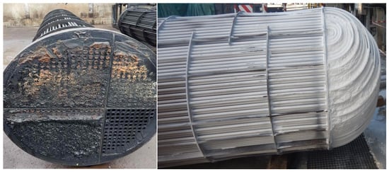
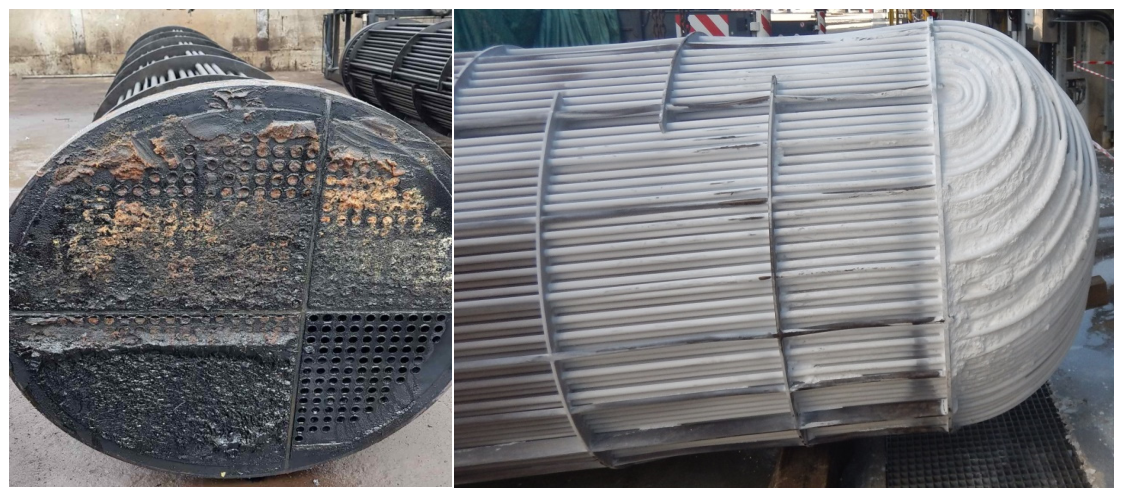
Among the most persistent operational challenges affecting heat exchangers in process industries is fouling [5], as illustrated in Figure 1. The gradual accumulation of deposits on heat transfer surfaces during long-term HEN operation can cause a substantial deterioration in the energy performance of an entire plant [6]. Consequently, fouling has become an important concern for HEN operators in several strategically significant industrial sectors, including oil refining and petrochemical production [7], as well as food-processing applications such as sugar production [8] and dairy processing [9]. From the perspective of large-scale energy management, researchers and industrial decision-makers regard fouling as a widespread problem occurring across multiple sectors, thereby requiring continuous monitoring and further investigation [10].

Figure 1. Fouling on heat transfer surfaces in heat exchangers in the petrochemical industry (photo: Marian Trafczynski).

The deterioration of heat recovery caused by fouling is primarily associated with a reduction in the steady-state rate of heat transfer [11]. In addition, fouling can cause unequal changes in the thermal performance of individual exchangers, which may disturb the interactions between units within the network [12]. These effects can be further complicated by changes in the dynamic behavior of the HEN [13]. To limit the resulting decline in heat recovery, different operational approaches can be implemented, including the model predictive control (MPC) method [14] and dedicated energy-efficient control strategies [15]. At the level of individual heat exchangers, fouling can be addressed through a variety of technological solutions, such as the use of advanced fouling-resistant materials and surface coatings during exchanger fabrication [16], as well as the implementation of self-cleaning heat exchanger technologies [17]. Another relatively straightforward approach is to compensate for the expected deterioration in performance by incorporating detailed heat exchanger sizing into HEN design and optimization [18]. Nevertheless, oversizing by itself does not eliminate the increase in energy consumption associated with progressive fouling, making appropriate operational strategies necessary [19]. Once the performance of the network or selected heat exchangers falls below an acceptable level, online cleaning of the affected equipment can be considered as an effective method for restoring heat transfer performance and maintaining energy recovery [20]. In contrast to the extensive literature on the influence of fouling on the heat transfer performance of exchangers, its influence on their dynamics and on the quality of control has received considerably less attention.

In Pinch Technology [21], the T-H (temperature–enthalpy) diagram is used to represent the composite curves of process streams. Their closest approach defines the so-called pinch point, which corresponds to the minimum temperature difference, ΔT_min. This parameter plays a fundamental role in the analysis and synthesis of heat exchanger networks because it directly influences the energy demand of an industrial process, the configuration of the HEN, and the required characteristics and size of individual heat exchangers. Reducing ΔT_min generally leads to lower entropy generation associated with heat transfer and can therefore improve the thermodynamic efficiency of the system.

The relationship between ΔT_min and the resulting energy performance depends on the type of industrial installation. In alignment with the primary and secondary laws of thermodynamics, typical effects observed in different sectors can be summarized as follows: (1) Chemical industry: A reduction in ΔT_min generally results in lower external heat demand. Typical values of ΔT_min are approximately 10–20 K. (2) Food-processing industry: Decreasing ΔT_min also reduces heat consumption, with commonly applied values in the range of 5–10 K. (3) Power generation and combined heat and power (CHP) plants: Lowering ΔT_min can contribute to an increase in electricity generation. Typical values are approximately 3–5 K. (4) Refrigeration systems: Reducing ΔT_min can decrease the mechanical energy required to drive the compressor. In such applications, ΔT_min values commonly fall within the range of 2–5 K.

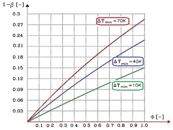
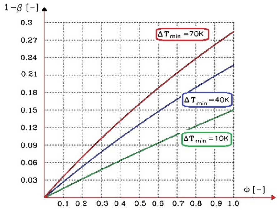
The choice of ΔT_min can also be relevant when considering the deterioration of heat transfer performance caused by fouling. Selecting an appropriate value during the design stage can help reduce the sensitivity of the heat transfer system to the formation of deposits on exchanger surfaces. The relationship between fouling and ΔT_min can, for example, be described using the function β = f(ΔT_min), where β represents the ratio between the heat transfer rate of a fouled exchanger, Q_f, measured before cleaning, and the corresponding heat transfer rate of a clean exchanger, Q_c [22]. Thus, β can be expressed as the relative heat transfer performance retained by the exchanger under fouled conditions. The variation of 1 − β as a function of ΔT_min is presented in Figure 2, illustrating the relationship between the selected minimum temperature difference and the loss of heat transfer capacity resulting from fouling.

Figure 2. Reduction in heat duty in a heat exchanger as a result of fouling [22]; ϕ—Biot fouling: ϕ = R_f·k_c, β = Q_f/Q_c.

In an earlier publication by Alabrudzinski and Markowski [23], the influence of ΔT_min on a heat and mass exchanger was analyzed, in which heat and mass exchange occur simultaneously, and the exchanger is affected by deposits. The analysis showed that for small values of ΔT_min, the influence of deposits on heat exchange and distillate purity can be neglected. To the best of the authors’ knowledge, quantitative descriptions of how fouling affects heat exchanger dynamics and control performance within a proportional–integral–derivative (PID) control loop were first provided in the authors’ own studies. Trafczynski et al. [24] investigated the impact of fouling on PID controller settings for individual heat exchangers, whereas Trafczynski et al. [25] examined its effect on PID control settings for a larger number of heat exchangers operating in a network with a control loop.

Fouling increases the thermal resistance of the heat transfer process, reducing the overall heat transfer coefficient and altering the exchanger’s dynamic characteristics. As a result, a PID controller tuned for the clean exchanger may no longer provide satisfactory control, and the effect of fouling on closed-loop performance depends on the operating point and the resulting process dynamics. The usual countermeasures, i.e., periodic retuning of the controller or advanced control such as MPC, are applied during operation, with the latter being costly and rarely used in industrial practice. In contrast, the minimum temperature difference ΔT_min, which characterizes the thermal driving force at the exchanger’s limiting point and determines its size and operating conditions, is selected at the design stage based on energy and economic criteria, without considering the exchanger’s controllability under fouling. Since a lower ΔT_min reduces the sensitivity of the heat duty to fouling (Figure 2), it can be expected that, although it requires a larger heat transfer area, it also reduces the sensitivity of the exchanger dynamics and control quality to deposits. To the best of the authors’ knowledge, this relationship has not been quantified so far. The motivation of this study is therefore to determine whether the choice of ΔT_min at the design stage can limit the need to retune PID controllers during operation. To this end, a dynamic model of a shell-and-tube crude oil preheater was used to compare the closed-loop responses, control-quality indices and stability margins of the clean and fouled exchangers for two values of ΔT_min (50 K and 10 K). The paper is organized as follows: Section 2 describes the steady-state and dynamic models, Section 3 presents the simulation results, and Section 4 summarizes the conclusions and practical implications.

2. Materials and Methods

2.1. Heat Exchanger in a Steady State

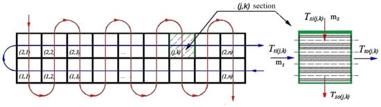
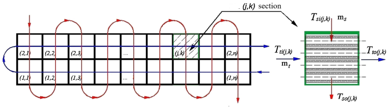
The mathematical model is based on energy balance equations describing the heat transfer processes occurring on both the tube and shell sides of the exchanger [24,25]. For the purpose of the analysis, the heat exchanger is divided into a number of sections corresponding to the partitions installed within the shell (Figure 3).

Figure 3. A diagram illustrating the division of a heat exchanger into sections. The red arrows refer to the hot stream flowing on the shell side of the heat exchanger, while the blue arrows refer to the cold stream flowing on the tube side.

According to [24], the model assumes that the fluids in each cell are perfectly mixed and have uniform temperatures; both fluids are incompressible with negligible pressure losses, and the thermophysical properties of the fluids and tube-wall materials remain constant. Heat conduction between cells, heat storage in the shell wall, changes in heat transfer coefficients between steady and transient conditions, and heat losses to the surroundings are also neglected.

These assumptions are considered reasonable for fully developed turbulent flow, where velocity and temperature profiles are relatively uniform and convective heat transfer dominates over conduction between cells. Although a complete heat exchanger model normally includes continuity, momentum, and energy equations for both fluids, as well as an energy equation for the tubes, the adopted simplifications eliminate the need to solve the continuity and momentum equations.

The heat balance of the medium in any section with coordinates (j,k) on the tube side (Figure 3) (for convenience, the coordinates (j,k) are omitted in the mathematical model [24]):

$$m_t\cdot c_t\cdot T_{ti}-m_t\cdot c_t\cdot T_{to}+n_b\cdot \mathsf{\Pi }\cdot d_1\cdot l\cdot {\alpha }_t\cdot (T_m-T_{to})=0$$

(1)

The heat balance of the medium on the shell side:

$$m_s\cdot c_s\cdot T_{si}-m_s\cdot c_s\cdot T_{so}-n_b\cdot \mathsf{\Pi }\cdot d_2\cdot l\cdot {\alpha }_s\cdot (T_{so}-T_m)=0$$

(2)

The model uses the following equation describing heat transfer in the exchanger:

$$Q=\int k_f\cdot \Delta T\cdot dF$$

(3)

$${\displaystyle \frac{1}{k_f}}={\displaystyle \frac{1}{k_c}}+R_f$$

(4)

$${\displaystyle \frac{1}{k_c}}={\displaystyle \frac{1}{{\alpha }_t}}+{\displaystyle \frac{1}{{\alpha }_s}}$$

(5)

where T—temperature, m—mass flow rate, c—specific heat, d₁ and d₂—inner and outer diameters of the tube, respectively, n_b—number of tubes in one pass, l—length of the tube in the section, Q—heat duty, ΔT—temperature difference, dF—heat exchange surface differential, k_f and k_c—overall heat transfer coefficients for the exchanger with deposits and the clean exchanger, respectively, R_f—fouling resistance, α_t, α_s—heat transfer coefficients on the tube and shell sides, respectively, indices: s—shell side, t—tube side, m—tube wall, i—inlet, o—outlet.

2.2. Heat Exchanger in a Dynamic State

The transient behavior of a shell-and-tube heat exchanger is modeled using a cell-based lumped-parameter approach [24]. This method relies on a set of simple equations and can accurately approximate the actual exchanger characteristics when a sufficiently large number of cells is used. It also allows different flow configurations to be represented for a given exchanger geometry.

The heat exchanger dynamics are represented by three ordinary differential equations that describe the energy balances of the tube wall and the shell-and-tube medium [24].

The heat balance of the medium in any section with coordinates (j,k) on the tube side (Figure 3) (for convenience, the coordinates (j,k) are omitted in the mathematical description):

$${\rho }_t{c}_t{V}_t{\displaystyle \frac{d{T}_{to}}{dt}}=m_t{c}_t{T}_{ti}-m_t{c}_t{T}_{to}+n_b\mathsf{\Pi }{d}_{1}l{\alpha }_t(T_m-T_{to})$$

(6)

The heat balance for the tube wall:

$${\rho }_m{c}_m{V}_m{\displaystyle \frac{d{T}_m}{dt}}=-\hspace{0.33em}{n}_b\mathsf{\Pi }{d}_{1}l{\alpha }_t(T_m-T_{to})+n_b\mathsf{\Pi }{d}_{2}l{\alpha }_s(T_{so}-T_m)$$

(7)

The heat balance of the medium on the shell side:

$${\rho }_s{c}_s{V}_s{\displaystyle \frac{d{T}_{so}}{dt}}=m_s{c}_s{T}_{si}-m_s{c}_s{T}_{so}-n_b\mathsf{\Pi }{d}_{2}l{\alpha }_s(T_{so}-T_m)$$

(8)

where ρ—density, V—volume.

After transformations, Equations (6)–(8) can be written in the following form:

$${\displaystyle \frac{d{T}_{to}}{dt}}=a_1\cdot {\dot{m}}_t\cdot (T_{ti}-T_{to})+a_2\cdot (T_m-T_{to})$$

(9)

$${\displaystyle \frac{d{T}_m}{dt}}=a_3\cdot (T_{to}-T_m)+a_4\cdot (T_{so}-T_m)$$

(10)

$${\displaystyle \frac{d{T}_{so}}{dt}}=a_5\cdot {\dot{m}}_s\cdot (T_{si}-T_{so})+a_6\cdot (T_m-T_{so})$$

(11)

where $a_1={\displaystyle \frac{1}{{\rho }_t\cdot V_t}}$, $a_2={\displaystyle \frac{n_b\cdot \mathsf{\Pi }\cdot d_1\cdot l\cdot {\alpha }_{ft}}{{\rho }_t\cdot c_t\cdot V_t}}$,$a_3={\displaystyle \frac{n_b\cdot \mathsf{\Pi }\cdot d_1\cdot l\cdot {\alpha }_{ft}}{{\rho }_m\cdot c_m\cdot V_m}}$, $a_4={\displaystyle \frac{n_b\cdot \mathsf{\Pi }\cdot d_2\cdot l\cdot {\alpha }_{fs}}{{\rho }_m\cdot c_m\cdot V_m}}$, $a_5={\displaystyle \frac{1}{{\rho }_s\cdot V_s}}$,$a_6={\displaystyle \frac{n_b\cdot \mathsf{\Pi }\cdot d_2\cdot l\cdot {\alpha }_{fs}}{{\rho }_s\cdot c_s\cdot V_s}}$, ${\alpha }_{ft}={\displaystyle \frac{{\alpha }_t}{{\alpha }_t\cdot R_{ft}+1}}$, ${\alpha }_{fs}={\displaystyle \frac{{\alpha }_s}{{\alpha }_s\cdot R_{fs}+1}}$.

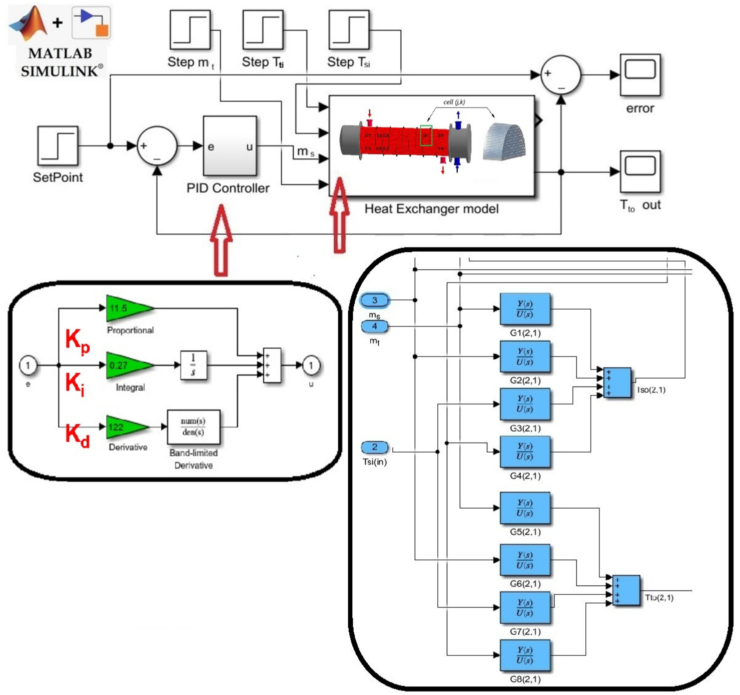
Solving the mathematical model equations establishes transfer relationships between disturbances introduced at the cell inlet and the resulting outlet temperature variations. The transfer function G(s) is a commonly applied representation of dynamic systems and is defined as the ratio of the Laplace transform of the output signal, y(s), to that of the input signal, u(s), under zero initial conditions: G(s) = y(s)/u(s). As illustrated in the right-hand section of Figure 3, each cell receives four input variables: the tube- and shell-side inlet temperatures, T_ti and T_si, and the corresponding mass flow rates, m_t and m_s. Two output variables are obtained: the tube- and shell-side outlet temperatures, T_to and T_so. Consequently, the dynamic model of each heat exchanger cell consists of eight transfer functions describing the relationships between the two output temperatures and each of the four inputs: G₁(s) = T_so(s)/m_t(s), G₂(s) = T_so(s)/m_s(s), G₃(s) = T_so(s)/T_si(s), G₄(s) = T_so(s)/T_ti(s), G₅(s) = T_to(s)/m_t(s), G₆(s) = T_to(s)/m_s(s), G₇(s) = T_to(s)/T_si(s), and G₈(s) = T_to(s)/T_ti(s).

The method for determining operator transfer functions is illustrated using the example of the transfer function: G₁(s) = T_so(s)/m_t(s). When determining G₁(s), attention must be paid to Equation (9), which involves the product of the controlled and input variables—namely, mass flow rate and temperature—and the resulting mathematical relationships are inherently nonlinear. To obtain a linear representation, Equation (9) can be approximated using a Taylor series expansion around the mean operating values of the variables:

$${\displaystyle \frac{d{T}_{to}}{dt}}=a_1\cdot {\dot{m}}_{tu}\cdot \left(T_{tiu}-T_{tou}\right)+a_2\cdot \left(T_{mu}-T_{tou}\right)+a_1\cdot {\dot{m}}_{tu}\cdot (T_{ti}-T_{tiu})-(a_1\cdot {\dot{m}}_{tu}+a_2)\cdot (T_{to}-T_{tou})+a_2\cdot (T_m-T_{mu})+a_1\cdot (T_{tiu}-T_{tou})\cdot ({\dot{m}}_t-{\dot{m}}_{tu})$$

(12)

The following substitutions were applied to Equations (10)–(12) to simplify the calculations:

$$\begin{array}{cccc}\begin{array}{c}X={\dot{m}}_t-{\dot{m}}_{tu}\hspace{0.33em},\\ \\ \end{array}& \begin{array}{c}Y=T_{so}-T_{sou}\hspace{0.33em},\hfill \\ T_{so}=Y+T_{sou}\hfill \\ d{T}_{so}=dY\hfill \end{array}& \begin{array}{c}W=T_{to}-T_{tou}\hspace{0.33em},\hfill \\ T_{to}=W+T_{tou}\hfill \\ d{T}_{to}=dW\hfill \end{array}& \begin{array}{c}Z=T_m-T_{mu}\hfill \\ T_m=Z+T_{mu}\hfill \\ d{T}_m=dZ\hfill \end{array}\end{array}$$

Next, the following system of equations was obtained:

$$\{\begin{array}{c}{\displaystyle \frac{dW}{dt}}=-(a_1\cdot {\dot{m}}_{tu}+a_2)\cdot W+a_1\cdot (T_{tiu}-T_{tou})\cdot X+a_2\cdot Z\hfill \\ {\displaystyle \frac{dZ}{dt}}=a_3\cdot (W-Z)+a_4\cdot (Y-Z)\hspace{1em}\hspace{1em}\hfill \\ {\displaystyle \frac{dY}{dt}}=-a_5\cdot {\dot{m}}_s\cdot Y+a_6\cdot (Z-Y)\hfill \end{array}$$

(13)

Applying the Laplace transform subsequently converts the differential equations into algebraic expressions:

$$\{\begin{array}{c}s\cdot \overline{W}=-(a_1\cdot {\dot{m}}_{tu}+a_2)\cdot \overline{W}+a_1\cdot (T_{tiu}-T_{tou})\cdot \overline{X}+a_2\cdot \overline{Z}\hfill \\ s\cdot \overline{Z}=a_3\cdot (\overline{W}-\overline{Z})+a_4\cdot (\overline{Y}-\overline{Z})\hspace{1em}\hspace{1em}\hfill \\ s\cdot \overline{Y}=-a_5\cdot {\dot{m}}_s\cdot \overline{Y}+a_6\cdot (\overline{Z}-\overline{Y})\hfill \end{array}$$

(14)

Finally, the system of Equation (14) allows the transfer functions for cell (j,k) to be derived in the following exemplary form [24]:

$$G_1\left(s\right)={\displaystyle \frac{{\overline{T}}_{so}}{{\overline{m}}_t}}={\displaystyle \frac{\overline{Y}}{\overline{X}}}={\displaystyle \frac{a_1{a}_3{a}_6\cdot (T_{tiu}-T_{tou})}{\left(s+a_1\cdot m_{tu}+a_2\right)\cdot \left[(s+a_3+a_4)\cdot (s+a_5\cdot m_{su}+a_6)-a_4{a}_6\right]-\left(s\cdot a_2{a}_3+a_2{a}_3{a}_5\cdot m_{su}+a_2{a}_3{a}_6\right)}}$$

(15)

2.3. Development and Implementation of a Dynamic Heat Exchanger Model in MATLAB/Simulink

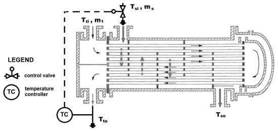
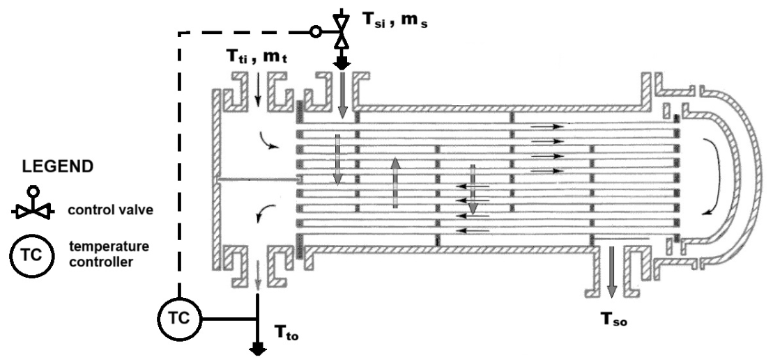
Figure 4 shows a diagram of the system with a PID temperature controller (TC) controlling the outlet temperature T_to of the oil on the tube side of the heat exchanger. In the PID-controlled heat exchanger system shown in Figure 4, the tube-side outlet temperature T_to serves as the controlled variable. Its value is regulated by adjusting the shell-side mass flow rate m_s, whereas the inlet temperatures of both streams, T_ti and T_si, together with the tube-side mass flow rate m_t, are treated as disturbance variables. Table 1 contains data for the heat exchanger shown in Figure 4.

Figure 4. Schematic diagram of a heat exchanger (AES-type exchanger according to TEMA [26]) with a PID system for temperature control T_to.

Table 1. Calculation parameters for the shell-and-tube heat exchanger for a CDU processing 440 t/h of crude oil.

Parameter	ΔTmin = 50 K	ΔTmin = 10 K
Exchanger classification by the TEMA 1	AES	AFS
Internal diameter of the shell, mm	1000	1500
Number of tubes	618	1390
Number of passes	2	4
External diameter of tubes, mm	25	25
Thickness of tube wall, mm	2.5	2.5
Tube pitch, mm	32	32
Layout	45°	45°
Baffle spacing, mm	250	250
Type of baffle	Single segmental	Single segmental
Clearances	TEMA 1 standards	TEMA 1 standards
Fouling resistance, value adopted from TEMA 1, m2K/W	0.00138	0.00138
Tube length, m	6	6
Oil flow rate on the shell side, t/h	56	56
Crude oil flow rate on the tube side, t/h	220	220
Temperature on the shell side, in/out, °C	143/88	143/88
Temperature on the tube side, in/out, °C	38/56	78/94
Viscosity on the shell side, in/out, mPa⋅s	0.293/0.466	0.293/0.466
Viscosity on the tube side, in/out, mPa⋅s	5.70/3.30	2.14/1.66
Conductivity on the shell side, in/out, W/(m⋅K)	0.097/0.109	0.097/0.109
Conductivity on the tube side, in/out, W/(m⋅K)	0.103/0.100	0.0968/0.0946
Density on the shell side, in/out, kg/m3	690/773	690/773
Density on the tube side, in/out, kg/m3	846/833	818/807
Specific heat on the shell side, in/out, J/(kg·K)	2471/2254	2471/2254
Specific heat on the tube side, in/out, J/(kg·K)	1924/2009	2098/2163
Heat transfer coefficient on the tube side, W/(m2K)	243	450
Heat transfer coefficient on the shell side, W/(m2K)	655	670
Conductivity of carbon steel tubes used in a shell-and-tube heat exchanger, W/(m·K)	50	50
Flow arrangement	1st pass: co-current 2nd pass: pure counter-current to the shell stream	1st, 3rd passes: co-current 2nd, 4th passes: counter-current to the shell stream

¹ Tubular Exchanger Manufacturers Association (TEMA) standards [26].

Before constructing the computer-aided dynamic model, it is necessary to establish a detailed block diagram of the heat exchanger. Such a representation facilitates the identification of relationships and interactions between individual exchanger cells. Since the heat exchanger is modeled as a series of interconnected cells arranged according to the selected flow configuration, the resulting block diagram can become relatively complex. The developed block diagram of the heat exchanger can subsequently be implemented in the MATLAB/Simulink environment and transformed into a simulation model—see Figure 5. An essential prerequisite for this process is the preparation of a database containing the steady-state operating parameters for each exchanger cell. In the present study, these data were obtained using Heat Transfer Research, Inc. (HTRI) software, HTRI Xchanger Suite version 7.3.2 [27], which was employed to calculate the steady-state parameter distribution of both fluids for the specified exchanger geometry [24]. Thus, HTRI Xchanger Suite 7.3.2 served as the source of the heat exchanger design and process data, whereas Matlab/Simulink version R2025b [28] was used for dynamic simulation and control analysis. The simulations were carried out using the ode45 solver with an automatic step size and a relative tolerance of 1 × 10⁻³ over a simulation time of 250 s, which is sufficient for all responses to reach steady state. The dynamic heat exchanger model in Simulink was validated using real-life measurements of the operating parameters, that is, temperatures and mass flows of both fluids, of a selected heat exchanger unit—see Section 3 in the previous work by the authors [24].

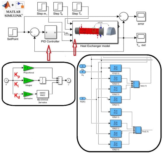
Figure 5. Simulink model of a heat exchanger system with a feedback PID controller.

This study examines two shell-and-tube heat exchangers: the first is an AES-type unit (with a ΔT_min of 50 K) currently operating in the crude distillation unit (CDU) processing 440 t/h of crude oil at the Orlen S.A. refinery in Poland. The second, an AFS-type exchanger (with a ΔT_min of 10 K), was newly designed by the authors using HTRI software. The design and geometric parameters were selected based on widely used TEMA [26] standards for industrial applications—see Table 1.

The analysis considers two limiting cases: a clean heat exchanger and a strongly fouled heat exchanger characterized by a fouling resistance of (R_f = 0.00138 m²K/W). This approach enables the assessment of the impact of substantial fouling on heat exchanger dynamics and control system quality and stability. However, intermediate fouling levels were not investigated in this work; for a systematic sensitivity analysis covering a wider range of fouling resistance values, please refer to previous work by the authors—see Figure 11 in source [24]. In this work, the analysis was conducted for a clean and a strongly fouled heat exchanger, and in this situation, the authors believe that, across different degrees of fouling, the results will not be groundbreaking.

2.4. Solution Procedure

The solution procedure consisted of five consecutive steps, which are described below.

Step 1: Steady-state design calculations. For each of the two cases (ΔT_min = 50 K and 10 K), the heat exchanger was designed with HTRI Xchanger Suite 7 for the process data in Table 1. The minimum temperature difference fixed the terminal temperature difference and, together with the assumed fouling resistance, determined the heat transfer area required for the given duty. This area was obtained by solving the system of Equations (1)–(5), in which the heat duty (3) was calculated by numerical integration over the exchanger sections, with the overall heat transfer coefficient given by Equations (4) and (5). The calculations were performed for a clean exchanger (R_f = 0) and for a fouled exchanger (R_f = 0.00138 m²K/W). From these calculations, the steady-state database of each cell was obtained: the inlet and outlet temperatures of both streams, the tube-wall temperature, the mass flow rates, the heat transfer coefficients and the fluid properties.

Step 2: Linearization and transfer functions. For each of the cells, Equations (6)–(8) were linearized around the steady-state operating point from Step 1 using a first-order Taylor series expansion (Equation (12)), and the coefficients a₁–a₆ were calculated from the cell data. The Laplace transform under zero initial conditions (Equation (14)) converted the linearized equations into algebraic ones, from which the eight transfer functions G₁(s)–G₈(s) of each cell were derived (Equation (15) gives G₁(s) as an example). The influence of fouling on the dynamics enters through: ${\alpha }_{ft}={\displaystyle \frac{{\alpha }_t}{{\alpha }_t\cdot R_{ft}+1}}$, ${\alpha }_{fs}={\displaystyle \frac{{\alpha }_s}{{\alpha }_s\cdot R_{fs}+1}}.$

Step 3: Simulation model. The cell transfer functions were implemented in MATLAB/Simulink R2025b and connected according to the exchanger’s flow arrangement (co-current and counter-current passes; Table 1, Figure 5). The tube-side outlet temperature T_to was the controlled variable, the shell-side mass flow rate m_s was the manipulated variable, and the inlet temperatures T_ti and T_si and the tube-side mass flow rate m_t were the disturbances (Figure 4). The PID controller was in parallel form—see Figure 5. The model was solved with the ode45 solver (variable step, relative tolerance 1 × 10⁻³) over 250 s, which is sufficient for all responses to reach a steady state. The model was validated against measurements from an industrial exchanger [24].

Step 4: Controller tuning and simulation scenarios. For the clean exchanger, the PID settings (K_p, T_i, T_d) were selected using the Ziegler–Nichols method [29] from the critical gain and the oscillation period of the closed loop. Then, the fouled exchanger was simulated with the same settings and, for ΔT_min = 50 K, with new settings obtained by repeating the Ziegler–Nichols procedure for the fouled exchanger. In each case, two scenarios were simulated: the response to a unit step of the set-point (set-point tracking) and the response to 10% step disturbances of m_t, T_ti and T_si, applied simultaneously and separately (disturbance rejection).

Step 5: Evaluation of control quality and stability. The responses were evaluated with the integral of the squared error (ISE, Equation (16)), the maximum overshoot σ_max (Equation (17)) and the settling time T_s (±5% of the steady-state value). In addition, the gain and phase margins were determined from the Bode plots of the open-loop linear G(s)_PID·G(s)_HE model for the clean and fouled exchanger under the original and retuned settings. The values obtained for ΔT_min = 50 K and 10 K were compared to assess the effect of ΔT_min on the control system’s sensitivity to fouling.

3. Study on the Influence of the Minimum Temperature Difference in a Heat Exchanger Under Fouling on the PID Temperature Controller Settings

According to results reported in previous studies [24], an increase in thermal resistance due to fouling alters the heat exchanger’s thermal inertia, thereby affecting its dynamic characteristics. These effects can be identified by analyzing the open-loop unit-step responses obtained from simulations performed at different stages of fouling development. The simulated responses indicate that, for all heat exchangers considered, fouling-induced changes in the heat transfer surfaces are reflected in the values of the gain K, delay time T_D, and time constant T₁. From a practical perspective, the changes in T_D are relatively minor. However, an increase in the time constant and the corresponding reduction in gain can significantly degrade the performance of the PID control system.

To maintain satisfactory control performance despite the progressive development of fouling, it is recommended to evaluate the effects of fouling on all three PID tuning parameters: the proportional, integral, and derivative gains (K_p, K_i, and K_d). The resulting controller settings should subsequently be assessed by analyzing the corresponding closed-loop responses [24].

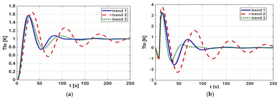
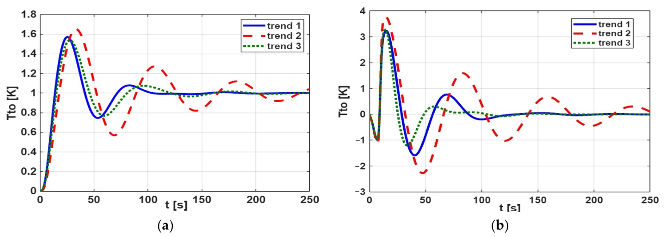
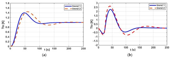
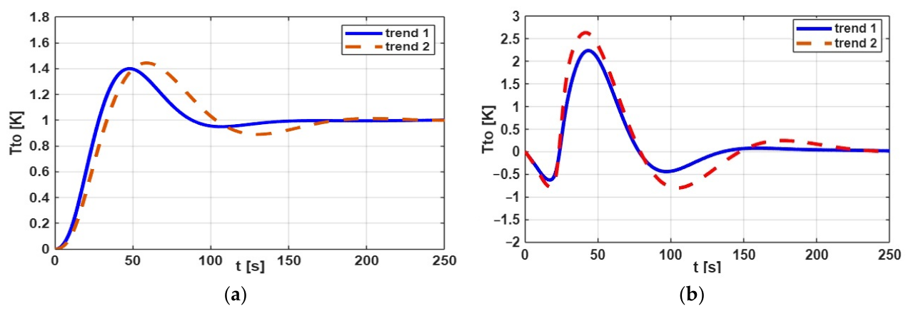
In this work, following the procedure in Section 2.4, a series of numerical simulations was performed using Simulink/MATLAB for the system shown in Figure 4. The calculation results are presented graphically in Figure 6 and Figure 7, as closed-loop step responses: Figure 6a and Figure 7a show the set-point tracking, and Figure 6b and Figure 7b show the disturbance rejection.

Figure 6. Closed-loop step responses, assuming ΔT_min = 50 K. (a) Set-point tracking—the responses to a unit input signal 1(t). (b) Disturbance rejection—temperature change at the tube outlet as a result of a 10% step disturbance in the m_t, T_ti, and T_si signals: trend 1—exchanger without fouling (R_f = 0 m²K/W), trend 2—exchanger with fouling (R_f = 0.00138 m²K/W), trend 3—exchanger with fouling (R_f = 0.00138 m² K/W) with new temperature controller settings.

Figure 7. Closed-loop step responses, assuming ΔT_min = 10 K. (a) Set-point tracking—the responses to a unit input signal 1(t). (b) Disturbance rejection—temperature change at the tube outlet as a result of a 10% step disturbance in the m_t, T_ti, and T_si signals: trend 1—exchanger without fouling (R_f = 0 m²K/W), trend 2—exchanger with fouling (R_f = 0.00138 m²K/W).

Figure 6a,b—trend 1 (blue solid lines)—show the change over time of the controlled temperature T_to for a heat exchanger without deposits. The TC controller settings were selected using the heuristic Ziegler–Nichols method [29], and the adopted values were: gain K_p = 21; integration time constant T_i = 19.1 s; derivative time constant T_d = 4.8 s. The calculations were performed for the parameter ΔT_min = 50 K.

Figure 6a,b (trend 2, red dashed lines) show the time evolution of the regulated temperature T_to for the exchanger with deposits, assuming the same controller settings as in trend 1. The observed course of changes indicates that the stability of the T_to signal has deteriorated significantly, and it is necessary to re-select the TC controller settings during heat exchanger operation. The course of the T_to signal, after changing the controller settings, is shown in Figure 6a,b—trend 3 (green dotted lines). The values of the new settings were also selected using the heuristic Ziegler–Nichols method [29]: K_p = 27; T_i = 22.5 s; T_d = 5.6 s—based on the critical gain and oscillation period. The retuning was not based on a separate numerical optimization procedure, and no explicit multi-objective optimization was performed.

Figure 7a,b—trend 1 (blue solid lines)—show the change over time of the controlled temperature T_to for a heat exchanger without deposits for the parameter ΔT_min = 10 K. The TC controller settings selected with the Ziegler–Nichols method are: gain K_p = 11.5; integration time constant T_i = 42.6 s; derivative time constant T_d = 10.6 s.

Figure 7a,b (trend 2, red dashed lines) show the change over time of the regulated temperature T_to for the heat exchanger with deposits, assuming the same controller settings as for the case in Figure 7a,b—trend 1. A comparison of the T_to signal course across trends 1 and 2 shows that the T_to curves have similar shapes. This means that, in that case (with parameter ΔT_min = 10 K), the influence of fouling on the heat exchanger’s dynamics is negligible. In this situation, there is no need to change the TC controller settings during heat exchanger operation.

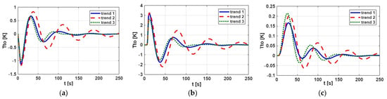
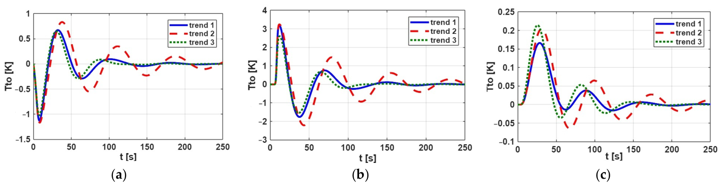
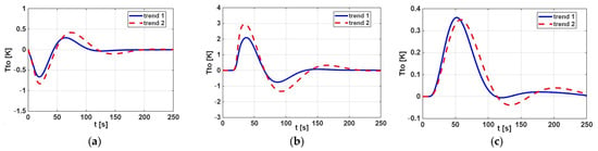
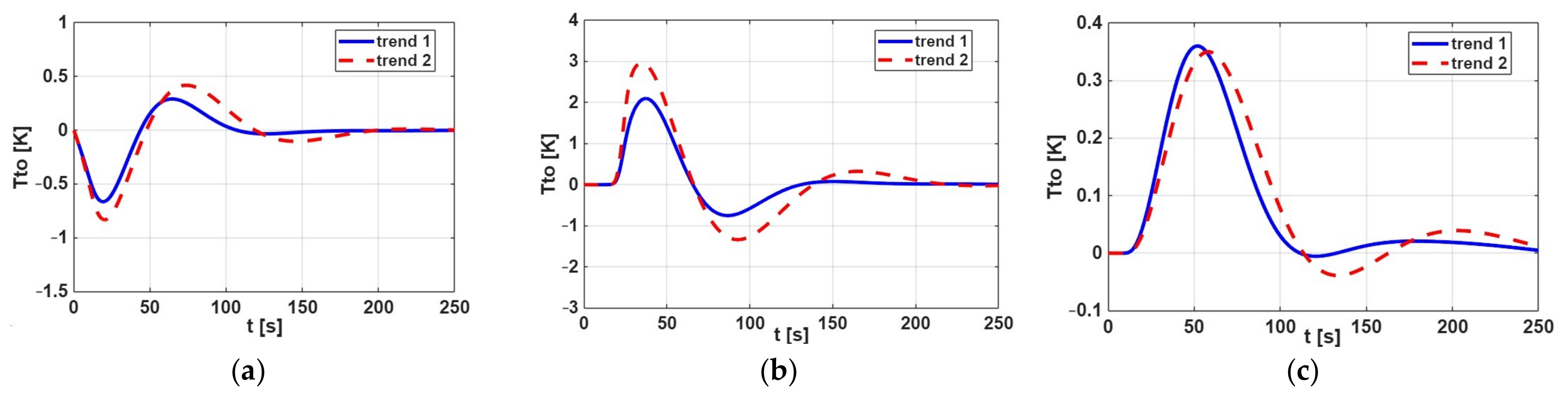
Since the number of disturbance rejection scenarios considered in Figure 6b and Figure 7b is limited—specifically, disturbances are introduced into the model as 10% step changes in the three signals m_t, T_ti and T_si simultaneously at t = 0 s—additional scenarios are presented in Figure 8 and Figure 9 to provide a more in-depth analysis of disturbance rejection performance. The disturbance rejection results obtained (shown in Figure 8 and Figure 9) are in full qualitative agreement with those shown in Figure 6b and Figure 7b, respectively; a quantitative assessment is presented below, based on control performance indices derived from closed-loop step responses.

Figure 8. Disturbance rejection, assuming ΔT_min = 50 K. (a) Temperature change at the tube outlet as a result of a +10% step disturbance in the crude oil flow rate on the tube side, m_t. (b) Temperature change at the tube outlet as a result of a +10% step disturbance in the inlet temperature on the tube side, T_ti. (c) Temperature change at the tube outlet as a result of a +10% step disturbance in the inlet temperature on the shell side, T_si. Trend 1—exchanger without fouling (R_f = 0 m²K/W), trend 2—exchanger with fouling (R_f = 0.00138 m²K/W), trend 3—exchanger with fouling (R_f = 0.00138 m² K/W) with new temperature controller settings.

Figure 9. Disturbance rejection, assuming ΔT_min = 10 K. (a) Temperature change at the tube outlet as a result of a +10% step disturbance in the crude oil flow rate on the tube side, m_t. (b) Temperature change at the tube outlet as a result of a +10% step disturbance in the inlet temperature on the tube side, T_ti. (c) Temperature change at the tube outlet as a result of a +10% step disturbance in the inlet temperature on the shell side, T_si. Trend 1—exchanger without fouling (R_f = 0 m²K/W) and trend 2—exchanger with fouling (R_f = 0.00138 m²K/W).

The control performance was further assessed using several analytical quality criteria. One of the criteria considered was the integral of the squared error (ISE), which is defined as follows:

$$\mathrm{I}\mathrm{S}\mathrm{E}= {\displaystyle \underset{t=0}{\overset{\infty }{\int }}}e{\left(t\right)}^{2}dt\approx t_s{\displaystyle \sum _{k=0}^{n_k}}{e\left(k\right)}^2$$

(16)

where e = w − y denotes the control error, defined as the difference between the set-point w and the controlled variable y. The parameter t_s represents the sampling time, while n_k denotes the total number of control steps. A lower ISE value indicates a smaller accumulated control error and, consequently, better closed-loop control performance.

Table 2 and Table 3 show the computed ISE values for set-point tracking and disturbance rejection of heat exchangers for two different values of the ΔT_min parameter. The data are presented for both the clean and fouled heat exchangers (trend 1 and trend 2). Based on the results presented in Table 2 and Table 3, the closed-loop performance of the heat exchanger with ∆T_min = 10 K was less affected by fouling than that at ∆T_min = 50 K. The differences in ISE values between the clean exchanger and the one with deposits are significantly smaller at ∆T_min = 10 K, except for the disturbance in the tube-side inlet temperature (Figure 8b and Figure 9b), where the increase is similar in both cases. For the clean exchanger, the set-point ISE is higher at ∆T_min = 10 K (18.4) than at 50 K (12.5).

Table 2. ISE values in set-point tracking.

Heat Exchanger	ΔTmin = 50 K	ΔTmin = 10 K
Without fouling—ISE in trend 1, Figure 6a and Figure 7a	12.5	18.4
With fouling—ISE in trend 2, Figure 6a and Figure 7a	21.9	23.4

Table 3. ISE values in the disturbance rejection.

Heat Exchanger	ΔTmin = 50 K	ΔTmin = 10 K
Without fouling—ISE in trend 1, Figure 6b and Figure 7b	152	136
With fouling—ISE in trend 2, Figure 6b and Figure 7b	336	216
Without fouling—ISE in trend 1, Figure 8a and Figure 9a	15.4	10.9
With fouling—ISE in trend 2, Figure 8a and Figure 9a	34.4	20.5
Without fouling—ISE in trend 1, Figure 8b and Figure 9b	97.6	112.8
With fouling—ISE in trend 2, Figure 8b and Figure 9b	254	261
Without fouling—ISE in trend 1, Figure 8c and Figure 9c	0.88	4.7
With fouling—ISE in trend 2, Figure 8c and Figure 9c	1.1	5.1

The control performance was also evaluated in terms of the maximum overshoot, defined as

$${\sigma }_{max}={\displaystyle \frac{y_{max}-y(\infty )}{y\left(\infty \right)-y\left(0\right)}}\times 100\%$$

(17)

where y_max denotes the maximum value attained by the controlled variable, y(0) is its initial value, and y(∞) represents the corresponding steady-state value. Another of the criteria considered was the settling time (T_s), defined as the time interval during which the step response remains within the tolerance margin of its steady-state value, usually y(∞) ± 5%. The analysis of σ_max and T_s was performed for both clean heat exchangers and exchangers subjected to fouling at two different values of the ΔT_min parameter, 10 K and 50 K—see Table 4 (only for set-point tracking).

Table 4. Maximum overshoot and settling time values in set-point tracking.

Heat Exchanger	ΔTmin = 50 K	ΔTmin = 10 K
Without fouling—σmax in trend 1, Figure 6a and Figure 7a	57%	40%
With fouling—σmax in trend 2, Figure 6a and Figure 7a	65%	44%
Without fouling—Ts in trend 1, Figure 6a and Figure 7a	91.8 s	107 s
With fouling—Ts in trend 2, Figure 6a and Figure 7a	231 s	159 s

An overshoot σ_max and the settling time T_s in the temperature response are undesirable because they degrade control performance. As illustrated in Figure 6 and Figure 7, the PID-controlled responses exhibit pronounced overshoots and longer settling times in the set-point tracking scenarios for the heat exchanger with ΔT_min = 50 K. The application of a lower parameter ΔT_min = 10 K substantially reduces these overshoots and the percentage increase in settling times (see Table 4) for the investigated heat exchanger, despite the progressive accumulation of fouling deposits during exchanger operation.

Nevertheless, closed-loop responses alone (evaluated for ISE, settling time, overshoot in disturbance rejection and set-point tracking performance) do not fully establish the overall quality of control or prove that the system is insensitive to fouling. This conclusion should be verified by analyzing the results presented in the Bode plot. Frequency-domain stability metrics, such as gain margin (GM) and phase margin (PM), should also be evaluated, as they are critical for assessing closed-loop safety under fouling drift.

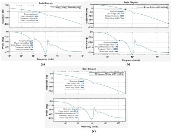
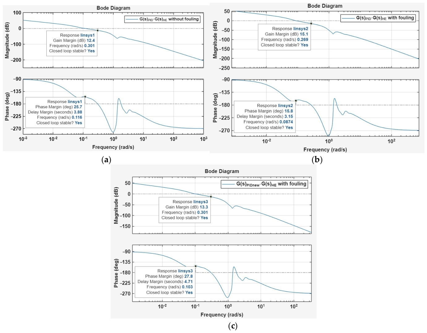
For the case with a minimum temperature difference of ΔT_min = 50 K, the Bode plot analysis (see Figure 10) revealed that fouling significantly affected the stability margins of the heat exchanger control system when the original PID controller settings (gain K_p = 21; integration time constant T_i = 19.1 s; derivative time constant T_d = 4.8 s) were retained. For the clean heat exchanger model in Figure 10a, the gain margin was 12.4 dB, and the phase margin was 25.7°. After introducing fouling—see Figure 10b—the gain margin increased to 15.1 dB, whereas the phase margin decreased to 15.8°, indicating reduced phase stability robustness and a greater susceptibility to oscillatory behavior. Retuning the PID controller (gain K_p = 27; integration time constant T_i = 22.5 s; derivative time constant T_d = 5.6 s) using the Ziegler–Nichols method improved the phase margin to 27.8°, while the gain margin decreased to 13.3 dB—see Figure 10c. These results demonstrated that controller retuning could compensate for the changes in heat exchanger dynamics caused by fouling under this operating condition.

Figure 10. Bode plots of the heat exchanger control system model (assumed ΔT_min = 50 K): (a) clean heat exchanger with the original PID controller settings; (b) fouled heat exchanger with the original PID controller settings; and (c) fouled heat exchanger with retuned PID controller settings obtained using the Ziegler–Nichols method to improve control performance and stability margins.

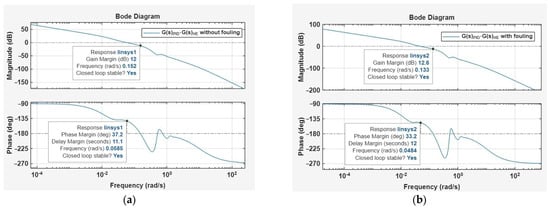
A different trend in the Bode plots was observed for ΔT_min = 10 K—see Figure 11. For the clean heat exchanger model in Figure 11a, the gain margin was 12.0 dB, and the phase margin was 37.2°. When fouling was introduced (see Figure 11b) while maintaining the same PID controller settings (gain K_p = 11.5; integration time constant T_i = 42.6 s; derivative time constant T_d = 10.6 s), the gain margin increased slightly to 12.6 dB, whereas the phase margin decreased only moderately to 33.8°. The changes in the gain and phase margins were therefore relatively small: the gain margin increased by 0.6 dB, while the phase margin decreased by 3.4°. These results suggest that, at ΔT_min = 10 K, the control system is less sensitive to changes in heat exchanger dynamics associated with fouling, and additional PID controller retuning may not be necessary.

Figure 11. Bode plots of the heat exchanger control system model (assumed ΔT_min = 10 K): (a) clean heat exchanger with the original PID controller settings; (b) fouled heat exchanger with the original PID controller settings.

This result should not be interpreted as an absence of fouling effects on heat transfer but rather as an indication that the control system tolerates the investigated changes without substantial deterioration in these stability measures.

Comparing the two operating conditions indicates that the influence of fouling on the control system’s stability depends on the value of ΔT_min. At ΔT_min = 50 K, the reduction in phase margin from 25.7° to 15.8° was substantial, indicating a pronounced change in the system’s dynamic characteristics and providing strong motivation for controller retuning. In contrast, at ΔT_min = 10 K, the phase margin decreased by only 3.4°, from 37.2° to 33.8°, while the gain margin remained almost unchanged. This suggests that the system exhibits greater robustness to fouling-related dynamic variations at the lower ΔT_min value.

In conclusion, the Bode diagram results indicate that the need for PID controller retuning depends on the heat exchanger’s operating conditions. For ΔT_min = 50 K, fouling considerably reduces the phase margin, and retuning the controller using the Ziegler–Nichols method improves the stability margins. For ΔT_min = 10 K, the gain and phase margins remain relatively close to those of the clean heat exchanger, suggesting that the original PID settings can be retained without a significant deterioration in stability robustness. Thus, the control system appears more tolerant of fouling-induced changes in dynamics at ΔT_min = 10 K than at ΔT_min = 50 K.

Overall, the assessment of the closed-loop response, including ISE, settling time, overshoot in set-point tracking, and disturbance rejection, demonstrates that an increase in fouling thermal resistance can significantly alter the dynamic response of the heat exchanger with a large parameter ΔT_min. If the controller tuning parameters remain unchanged, fouling may result in oscillations of the controlled temperature, an excessively slow response to set-point changes, and substantial temperature overshoots. These adverse effects can be mitigated by appropriately tuning the PID gains. Alternatively, during the design stage of heat exchangers, the above aspect should be taken into account by selecting the appropriate lower ΔT_min parameter in the heat and flow calculations for the exchanger.

The aim of this article was to examine whether the choice of ΔT_min at the design stage can reduce the influence of fouling on the control system. As shown in Figure 2, for small values of the minimum temperature difference, the exchanger’s heat duty is less affected by fouling. The simulation results presented above indicate that the control system is also less sensitive to fouling in this case. This observation may be useful to design engineers, who can take expected fouling-related changes in dynamics into account when selecting ΔT_min, in addition to the required process parameters. The conclusions are based on two exchanger models with different ΔT_min values and should be verified for other cases.

In an industrial heat exchanger network, interactions between adjacent units may affect operating conditions and control performance. In this study, these interactions are represented indirectly by perturbations in the inlet temperature of the selected heat exchanger—see Figure 9b,c, reflecting changes in upstream operating conditions. The simulation results in Figure 11a,b indicate that at a relatively low minimum temperature difference (ΔT_min = 10 K), the heat exchanger exhibits robustness to fouling-related dynamic changes, maintaining similar gain and phase margins under clean and fouled conditions with unchanged PID controller settings. This suggests that the control system can tolerate the investigated inlet temperature disturbances without requiring additional controller retuning.

4. Concluding Remarks

This paper examined how the minimum temperature difference, ΔT_min, selected at the design stage affects the dynamic behavior of a shell-and-tube heat exchanger under fouling and the settings of its PID temperature controller. A typical industrial heat exchanger has time-varying dynamics because deposits form on the heat transfer surface during operation. The simulations for a crude oil preheater showed that this effect depends strongly on ΔT_min.

At ΔT_min = 50 K, fouling (R_f = 0.00138 m²K/W) markedly degraded the closed-loop response when the original PID settings were retained. The set-point ISE increased from 12.5 to 21.9, the settling time from 91.8 s to 231 s, and the overshoot from 57% to 65%. The phase margin fell from 25.7° to 15.8°, so the controller had to be retuned during operation. At ΔT_min = 10 K, the same fouling produced much smaller changes: the set-point ISE increased from 18.4 to 23.4, the settling time from 107 s to 159 s, and the overshoot from 40% to 44%. The phase margin decreased by only 3.4° (from 37.2° to 33.8°), and the gain margin changed by 0.6 dB. The original settings could therefore be retained. For the combined 10% disturbance, the ISE grew by a factor of 2.2 at ΔT_min = 50 K and by a factor of 1.6 at ΔT_min = 10 K. The benefit was less clear for the inlet temperature disturbance on the tube side, where the increase in ISE was similar across both ΔT_min values. Without fouling, the 10 K design also gave a somewhat higher set-point ISE and a longer settling time than the 50 K design.

Retuning the controller with the Ziegler–Nichols method restored the phase margin at ΔT_min = 50 K to 27.8°. This remains below the commonly preferred range of approximately 45–60°, so further tuning may be beneficial when greater robustness is required. At ΔT_min = 10 K, the original settings provided satisfactory stability margins for both the clean and the fouled exchanger.

From a practical standpoint, the results support a simple design guideline: where the economics of the process allow it, a lower ΔT_min should be preferred in the thermal calculations of exchangers that are prone to fouling because it reduces the need to retune PID controllers during operation. A lower ΔT_min leads to a larger heat transfer area, so this benefit should be weighed against the investment cost. The guideline does not require dynamic simulations from the designer. Such simulations are a research tool, used here to quantify the effect, and they can optionally be used to verify the choice of ΔT_min in particularly critical applications. PID controllers remain the standard in industry, whereas advanced or adaptive control strategies are rarely applied because of their cost and operational complexity. For this reason, reducing the sensitivity of the exchanger itself to fouling is an attractive complement to controller tuning.

The study has limitations. It covers one exchanger, two values of ΔT_min, one level of fouling, and a single tuning method (Ziegler–Nichols), so the conclusions should not be generalized without further verification. Future research may extend the analysis to other exchangers and fouling levels, to exchangers operating in networks, and to other tuning methods, such as Cohen–Coon, Tyreus–Luyben and optimization-based approaches. Such comparisons should consider stability margins, transient response, disturbance rejection and robustness to fouling-induced changes in exchanger dynamics.

References

- Bisht, P.S.; Gopalakrishnan, B.; Dahal, R.; Li, H.; Liu, Z. Parametric Energy Efficiency Impact Analysis for Industrial Process Heating Furnaces Using the Manufacturing Energy Assessment Software for Utility Reduction. Processes 2024, 12, 737. [Google Scholar] [CrossRef] [Scilit]
- Boldyryev, S.; Ivashchuk, O.S.; Krajačić, G.; Atamanyuk, V.M. Review of Challenges in Heat Exchanger Network Development for Electrified Industrial Energy Systems. Energies 2025, 18, 3685. [Google Scholar] [CrossRef] [Scilit]
- Pavão, L.V.; Costa, C.B.; Ravagnani, M.A. Multiple utilities targeting in energy integration considering rigorous temperature-enthalpy relations. Chem. Eng. Sci. 2023, 276, 118763. [Google Scholar] [CrossRef] [Scilit]
- Saeb Gilani, B.; Morosuk, T. Heat Exchanger Networks: Applications for Industrial Integrations. Energies 2025, 18, 3021. [Google Scholar] [CrossRef] [Scilit]
- Ou, R.; Ramasamy, M.G.; Rozali, N.E.M.; Mahadzir, S.; Ghumman, A.S.M.; Qureshi, A.H. Modeling Strategies for Crude Oil-Induced Fouling in Heat Exchangers: A Review. Processes 2023, 11, 1036. [Google Scholar] [CrossRef] [Scilit]
- Dorosevas, V.; Lousada, S.; Jankauskienė, D. Fouling-Induced Degradation and Pneumoshock Cleaning Strategy for Shell-and-Tube Heat Exchangers in Oil Refining Thermal Management. Processes 2026, 14, 1442. [Google Scholar] [CrossRef] [Scilit]
- Kamalifar, S.; Peyghambarzadeh, S.M.; Azizi, S.; Jamali-Sheini, F. Experimental study on crude oil fouling in preheat exchangers at different operating conditions. Therm. Sci. Eng. Prog. 2023, 39, 101742. [Google Scholar] [CrossRef] [Scilit]
- Abo, L.D.; Hailegiorgis, S.M.; Gindaba, G.T.; Jayakumar, M.; Prabhu, S.V. A Comprehensive Review on Fouling of Heat Transfer Units in Sugar Factory Ethanol Plant: Mechanisms and Mitigation Methods. Qual. Manag. 2024, 34, e70003. [Google Scholar] [CrossRef] [Scilit]
- Tarapata, J.; Murphy, T.R.; Finnegan, E.W.; O’Callaghan, T.F.; O’Mahony, J.A. Approaches for Measuring and Predicting Fouling During Thermal Processing of Dairy Solutions. Compr. Rev. Food Sci. Food Saf. 2025, 24, e70209. [Google Scholar] [CrossRef] [Scilit] [PubMed]
- Villa, L.; Zanini Brusamarello, C. Application of machine learning in monitoring fouling in heat exchangers in chemical engineering: A systematic review. Can. J. Chem. Eng. 2025, 103, 1786–1801. [Google Scholar] [CrossRef] [Scilit]
- Ilyunin, O.; Bezsonov, O.; Rudenko, S.; Serdiuk, N.; Udovenko, S.; Kapustenko, P.; Plankovskyy, S.; Arsenyeva, O. The neural network approach for estimation of heat transfer coefficient in heat exchangers considering the fouling formation dynamic. Therm. Sci. Eng. Prog. 2024, 51, 102615. [Google Scholar] [CrossRef] [Scilit]
- Ben-Mansour, R.; El-Ferik, S.; Al-Naser, M.; Qureshi, B.A.; Eltoum, M.A.M.; Abuelyamen, A.; Al-Sunni, F.; Ben Mansour, R. Experimental/Numerical Investigation and Prediction of Fouling in Multiphase Flow Heat Exchangers: A Review. Energies 2023, 16, 2812. [Google Scholar] [CrossRef] [Scilit]
- Hatte, S.; Stoddard, R.; Pitchumani, R. Generalized analysis of dynamic flow fouling on heat transfer surfaces. Int. J. Heat Mass Transf. 2022, 188, 122573. [Google Scholar] [CrossRef] [Scilit]
- Ren, C.; Han, J.; Chen, C.; Yang, C. Multi-period optimization embedded dynamic path-constrained model predictive control for heat exchanger networks under fouling conditions. Appl. Therm. Eng. 2025, 280, 128220. [Google Scholar] [CrossRef] [Scilit]
- Bakošová, M.; Oravec, J. Robust model predictive control for heat exchanger network. Appl. Therm. Eng. 2014, 73, 924–930. [Google Scholar] [CrossRef] [Scilit]
- He, Z.; Lian, W.; Lv, Y.; Duan, Z.; Fan, Z. Review of the Mitigation Scale Performance of Anti-Fouling Coatings Surface Characteristics on Industrial Heat Exchange Surfaces. Coatings 2026, 16, 40. [Google Scholar] [CrossRef] [Scilit]
- Chen, Z.; Zhou, Y.; Yang, Z.; Song, Z.; Li, J.; Zhang, G.; Han, F. A new preparation method of the dual scale surface microstructures with self-cleaning and efficient boiling heat transfer based on wire electrical discharge machining and laser etching. Appl. Therm. Eng. 2025, 279, 127822. [Google Scholar] [CrossRef] [Scilit]
- Yang, Z.; Zhang, N. Heat exchanger network design and optimization. In Process Systems Engineering Tools for Industrial Decarbonization; Elsevier: Amsterdam, The Netherlands, 2026; pp. 253–279. [Google Scholar] [CrossRef] [Scilit]
- Ishiyama, E.M.; Juhel, C.; Aquino, B.; Hagi, H.; Pugh, S.J.; Gomez Suarez, E.; Kennedy, J.; Zettler, H.U. Advanced Fouling Management through Use of HTRI SmartPM: Case Studies from Total Refinery CDU Preheat Trains. Heat Transf. Eng. 2022, 43, 1365–1377. [Google Scholar] [CrossRef] [Scilit]
- Suarez, E.G.; Kennedy, J.; Pugh, S.J.; Ishiyama, E.M. Fouling Management at TotalEnergies through Use of HTRI SmartPM: Case Study of a Project Proposal for Cleaning Schedule Optimization. Heat Transf. Eng. 2024, 45, 1357–1368. [Google Scholar] [CrossRef] [Scilit]
- Linnhoff, B.; Townsend, D.W.; Boland, D.; Hewitt, G.F.; Thomas, B.E.A.; Guy, A.R.; Marsland, R.H. A User Guide on Process Integration for the Efficient Use of Energy; Institution of Chemical Engineers: Rugby, UK, 1982. [Google Scholar]
- Markowski, M. Reconstruction of a heat exchanger network under industrial constraints—The case of a crude distillation unit. Appl. Therm. Eng. 2000, 20, 1535–1544. [Google Scholar] [CrossRef] [Scilit]
- Alabrudzinski, S.; Markowski, M. Impact of temperature approach on the behavior of the rectification heat and mass exchanger under fouling constraints. Energy Rep. 2022, 8, 7312–7324. [Google Scholar] [CrossRef] [Scilit]
- Trafczynski, M.; Markowski, M.; Alabrudziński, S.; Urbaniec, K. The influence of fouling on the dynamic behavior of PID-controlled heat exchangers. Appl. Therm. Eng. 2016, 109, 727–738. [Google Scholar] [CrossRef] [Scilit]
- Trafczynski, M.; Markowski, M.; Kisielewski, P.; Urbaniec, K.; Wernik, J.A. Modelling Framework to Investigate the Influence of Fouling on the Dynamic Characteristics of PID-Controlled Heat Exchangers and Their Networks. Appl. Sci. 2019, 9, 824. [Google Scholar] [CrossRef] [Scilit]
- TEMA. Tubular Exchanger Manufacturers Association, Standards of the Tubular Exchanger Manufacturers Association, 8th ed.; TEMA: New York, NY, USA, 1999. [Google Scholar]
- Heat Transfer Research, Inc. HTRI Xchanger Suite 7.3.2; Heat Transfer Research, Inc.: College Station, TX, USA, 2013. [Google Scholar]
- The MathWorks, Inc. MATLAB and Simulink R2025b; The MathWorks, Inc.: Natick, MA, USA, 2025. [Google Scholar]
- Ziegler, J.G.; Nichols, N.B. Optimum settings for automatic controllers. Trans. ASME. 1942, 64, 759–765. [Google Scholar] [CrossRef] [Scilit]
Disclaimer/Publisher’s Note: The statements, opinions and data contained in all publications are solely those of the individual author(s) and contributor(s) and not of MDPI and/or the editor(s). MDPI and/or the editor(s) disclaim responsibility for any injury to people or property resulting from any ideas, methods, instructions or products referred to in the content. |
© 2026 by the authors. Licensee MDPI, Basel, Switzerland. This article is an open access article distributed under the terms and conditions of the Creative Commons Attribution (CC BY) license.