Ultra-Short-Term Wind Power Forecasting Based on Adaptive Selective Denoising and TimeMixer-Mamba

Abstract

To improve the accuracy of ultra-short-term wind power forecasting, this paper proposes a forecasting method based on adaptive selective denoising and TimeMixer-Mamba. First, variational mode decomposition (VMD) decomposes the original wind power sequence into multiple intrinsic mode functions (IMFs). A comprehensive noise score combining the correlation coefficient and sample entropy is then constructed to adaptively identify high-noise IMFs, which are selectively denoised using wavelet packet decomposition (WPD) and an adaptive soft threshold (AST). Subsequently, TimeMixer-Mamba is developed to capture multiscale temporal patterns, long-term dependencies, and abrupt changes in wind power. The improved whale optimization algorithm (IWOA) is further employed to optimize the key model hyperparameters. The proposed method is evaluated on a real-world wind farm dataset with a 15-min forecasting horizon and a chronological 6:2:2 training/validation/test split. The proposed method achieves an RMSE of 1.89, an MAE of 0.97, and an R² of 0.9855. The inclusion of WPD-AST provides a modest additional improvement, reducing RMSE from 1.93 to 1.89 and MAE from 1.01 to 0.97. These results support the effectiveness of the proposed method for ultra-short-term wind power forecasting within the evaluated setting.

1. Introduction

Driven by the “dual-carbon” targets and the ongoing development of a new power system, wind power, as a renewable energy source with substantial development potential, has seen continued growth in both installed and grid-connected capacity [1]. However, wind energy resources are highly sensitive to meteorological conditions, and wind power generation sequences exhibit strong randomness, nonlinearity, and nonstationarity, posing substantial challenges to power system dispatch, secure operation, and reserve capacity allocation. Therefore, accurate and reliable wind power forecasting is essential for improving wind power integration, optimizing power system dispatch, and ensuring secure and stable power system operation [2,3].

Given the pronounced volatility and nonstationarity of wind power time series, signal decomposition techniques have been widely adopted for wind power forecasting. Variational Mode Decomposition (VMD) enables adaptive signal decomposition by formulating a constrained variational optimization problem and has demonstrated clear advantages in mitigating mode mixing [4,5]. Sun et al. [6] integrated VMD with deep learning models and demonstrated that decomposing raw power or wind speed time series into distinct modal components can effectively reduce nonstationarity and noise interference, thereby improving the accuracy and stability of wind power forecasting. However, the relative contributions of effective power fluctuations and random noise vary across modal components. Applying a uniform denoising strategy to all modal components may result in excessive smoothing and the loss of useful information in relatively low-noise modes. To address this issue, Yang et al. [7] employed Improved Complete Ensemble Empirical Mode Decomposition with Adaptive Noise (ICEEMDAN) and permutation entropy-based reconstruction to decompose wind power output into three components: random, oscillatory, and trend. The noise component is then forecast separately to reduce its interference with the forecasting of the main trend. However, this method primarily mitigates the influence of noise on main-trend forecasting through independent modeling of the noise component, rather than directly suppressing noise in the input data. Chang et al. [8] first applied CEEMDAN for initial decomposition, followed by entropy-based noise screening, and subsequently employed wavelet packet decomposition (WPD) for secondary denoising using a fixed threshold. While this method is simple to implement and computationally efficient, its noise identification relies on empirically determined values or fixed thresholds, which limits its adaptability to signals with different noise characteristics. Therefore, an adaptive selective denoising method integrating VMD, WPD, and adaptive soft threshold (AST) is proposed in this study. Noise is selectively localized, while the soft-threshold value is dynamically adjusted according to the signal-to-noise ratio (SNR) of each subband, enabling a better balance between preserving useful nonlinear information and effectively suppressing noise.

Early research on wind power forecasting primarily relied on traditional statistical models. With the rapid development of artificial intelligence, Liu et al. [9] demonstrated that neural network-based forecasting methods can effectively extract complex temporal patterns from wind power data and have achieved considerable progress. Long Short-Term Memory (LSTM) networks effectively alleviate the vanishing gradient problem of conventional Recurrent Neural Networks (RNNs) and have demonstrated good performance in time series forecasting tasks. However, their ability to capture long-range temporal dependencies remains limited [10]. To improve global feature extraction, Transformer models based on the self-attention mechanism have been introduced into wind power forecasting. Studies have shown that Transformers can effectively capture long-range dependencies in time series [11], but their ability to characterize local dynamic variations remains relatively limited [12]. More recently, Mamba has been introduced into wind power forecasting to efficiently model long-range dependencies and abrupt fluctuations in wind power time series. By serving as the primary feature extractor in a dual-branch architecture, Mamba can effectively extract global dynamic information. Yang and Zhang [13] reported that Mamba-based architectures can be effectively applied to medium- and short-term wind power forecasting. In parallel, Gong et al. [14] employed TimeMixer for multistep prediction and demonstrated its ability to model temporal information through multiscale mixing. They further developed an adaptive multiscale short-term wind power forecasting framework based on TimeMixer and a Mixture-of-Experts architecture, demonstrating the potential of TimeMixer for multiscale temporal modeling in wind power forecasting. However, existing studies generally investigate TimeMixer-based multiscale modeling and Mamba-based state-space modeling separately. Therefore, considering the complementary characteristics of TimeMixer and Mamba, this study employs TimeMixer to construct a multiscale temporal modeling framework and introduces Mamba to improve the capture of long-range dependencies and abrupt fluctuations. By integrating multiscale temporal modeling and selective state-space modeling, the proposed framework is expected to improve the representation of both stable temporal patterns and rapidly changing dynamics in wind power sequences.

In addition, the predictive performance of deep learning models is highly dependent on appropriate hyperparameter selection. Swarm intelligence optimization algorithms, such as Gray Wolf Optimization (GWO), Particle Swarm Optimization (PSO), and Sparrow Search Algorithm (SSA), have therefore been widely employed for automatic hyperparameter selection in neural network models [15,16,17]. Among these methods, Li et al. [18] employed the Whale Optimization Algorithm (WOA) to optimize the hyperparameters of a BiLSTM model. However, conventional WOA suffers from relatively slow convergence and a tendency to become trapped in local optima when searching complex and high-dimensional solution spaces. To overcome these limitations, Bozorgi and Yazdani [19] incorporated a mutation operator from Differential Evolution into WOA and introduced adaptive search-mode switching and population reinitialization mechanisms, thereby enhancing its global search capability and mitigating premature convergence and entrapment in local optima.

Table 1 compares the methodological designs of representative related studies with the proposed method. It should be noted that this comparison is intended to clarify design differences and overlaps rather than to rank numerical performance across papers.

Table 1. Methodological comparison with related forecasting approaches.

Study	Method	Advantage	Limitation	Difference from This Study
Sun et al. [6]	VMD + CNN-BiLSTM	Noise reduction and feature extraction	May over-smooth low-noise IMFs	Selective denoising of high-noise IMFs
Yang et al. [7]	ICEEMDAN + Permutation Entropy	Component identification	Limited direct noise suppression	Adaptive denoising before forecasting
Chang et al. [8]	CEEMDAN + PE + WPD	Efficient signal denoising	Limited threshold adaptivity	Adaptive threshold based on subband characteristics
Liu et al. [9]	TCN-LSTM	Temporal feature extraction	Limited multiscale and long-range modeling	TimeMixer-Mamba for multiscale and long-range modeling
Ahmadi et al. [10]	Kalman Filter + Deep Residual Learning + BiLSTM	Filtering and temporal modeling	Limited long-range modeling	TimeMixer-Mamba for multiscale and long-range dependencies
Yin and Liu [11]	BERT + Quantum Dual-Stage Attention + BiGRU + Diffusion	Long-term dependency modeling	Complex architecture	TimeMixer for multiscale representation
Jia et al. [12]	FPQ-iTransformer	Global dependency modeling	Not designed for wind power	Wind-power-oriented TimeMixer-Mamba
Yang and Zhang [13]	LCNN-Mamba	Local and long-range feature extraction	Mainly relies on Mamba	TimeMixer-Mamba for complementary modeling
Gong et al. [14]	TimeMixer + MoE	Multiscale temporal modeling	Additional model complexity	Mamba for long-range dependency modeling
Li et al. [18]	WOA + RNN-BiLSTM	Automatic parameter optimization	Search efficiency depends on strategy	IWOA for TimeMixer-Mamba optimization

Based on this analysis, this paper proposes an ultra-short-term wind power forecasting method based on adaptive selective denoising and TimeMixer-Mamba. First, VMD is employed to decompose the raw wind power time series into modal components at different frequency scales. A comprehensive noise score is then constructed based on the correlation coefficient and sample entropy, jointly accounting for each modal component’s correlation with the original signal and its complexity, to adaptively identify high-noise IMFs. Second, WPD is applied exclusively to the identified high-noise modes for further multiscale decomposition, and adaptive soft thresholds are determined using the Median Absolute Deviation (MAD) and the subband signal-to-noise ratio to achieve frequency-dependent selective denoising. During the forecasting stage, a TimeMixer-Mamba hybrid model is constructed to jointly capture multiscale temporal patterns, long-range dependencies, and abrupt fluctuations in wind power sequences. The Improved Whale Optimization Algorithm (IWOA) is further employed to optimize the key hyperparameters of the forecasting model. Finally, the effectiveness of the proposed method is evaluated in terms of forecasting accuracy through comparative and ablation experiments using real-world wind farm data.

2. Adaptive Selective Denoising Method

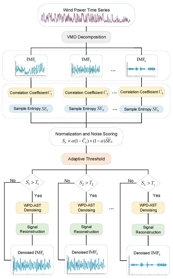
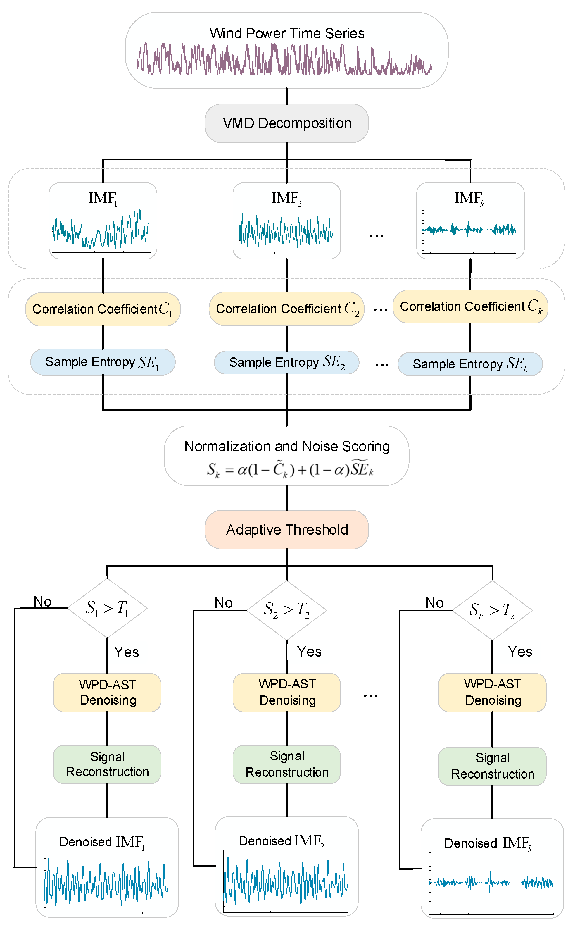
To mitigate the adverse effects of random noise in wind power time series on forecasting performance while minimizing the loss of useful information due to excessive denoising, this study proposes an adaptive selective denoising method based on VMD-WPD-AST. First, VMD is employed to decompose the raw wind power time series into modal components at different frequency scales, and high-noise IMFs are adaptively identified based on correlation coefficients and sample entropy. Subsequently, WPD-AST is applied exclusively to the identified high-noise IMFs for adaptive denoising, while relatively low-noise IMFs are retained to preserve useful information. Finally, the denoised and retained IMFs are reconstructed to obtain the processed wind power series. The overall procedure is illustrated in Figure 1.

Figure 1. VMD-WPD-AST denoising flowchart.

2.1. Variational Mode Decomposition

VMD is a non-recursive, adaptive signal processing technique that decomposes an original signal into multiple IMFs by constructing and solving a constrained variational optimization problem. Each IMF is characterized by a specific center frequency and finite bandwidth [20]. The corresponding variational problem can be formulated as follows:

$${\min }_{\{u_k\},\{{\omega }_k\}}\left\{{\displaystyle \sum _{k=1}^K{‖{\partial }_t\left[\left(\delta (t)+\frac{j}{\mathit{\pi t}}\right)\ast u_k(t)\right]e^{-j{\omega }_{k}t}‖}_2^2}\right\}$$

(1)

$$\mathrm{s}.\mathrm{t}. {\displaystyle \sum _{k=1}^K{u}_k}(t)=P(t)$$

(2)

where P(t) denotes the original wind power sequence; K denotes the number of decomposition modes; u_k(t) denotes the k-th modal component; ω_k denotes its corresponding center frequency; δ(t) denotes the Dirac delta function; ∗ denotes the convolution operation; and ∂_t denotes the partial derivative with respect to time.

Each modal component u_k(t) can be regarded as an amplitude-modulated and frequency-modulated signal in the time domain:

u_k(t) = A_k(t)cos[φ_k(t)]

(3)

where A_k(t) denotes the non-negative envelope amplitude; and φ_k(t) denotes the instantaneous phase function. By introducing the penalty factor α and the Lagrange multiplier λ(t), the constrained variational problem is transformed into an unconstrained form. The alternating direction method of multipliers (ADMM) is then employed to iteratively solve for each mode and its corresponding center frequency.

2.2. IMF Composite Noise Scoring and Classification

Following VMD, the proportions of effective power fluctuation information and random noise vary across IMFs. Therefore, directly applying a uniform denoising strategy to all modes may remove useful fluctuation information from relatively low-noise IMFs. To address this issue, this study further characterizes the noise properties of each IMF from two complementary perspectives: linear correlation and nonlinear complexity, using the correlation coefficient and sample entropy, respectively.

First, the Pearson correlation coefficient C_k between each IMF and the original wind power time series is calculated to quantify the linear contribution of each mode to the original power sequence. Subsequently, sample entropy is introduced as a complementary noise indicator to characterize the complexity and irregularity of each IMF [21]:

$$S{E}_k\triangleq -\ln \left({\displaystyle \frac{{\displaystyle \sum _{i=1}^{N-2}{\displaystyle \sum _{j\ne i}1}}\{{\max }_{0\le q\le 2}|u_k(i+q)-u_k(j+q)|\le r\}}{{\displaystyle \sum _{i=1}^{N-1}{\displaystyle \sum _{j\ne i}1}}\{{\max }_{0\le q\le 1}|u_k(i+q)-u_k(j+q)|\le r\}}}\right)$$

(4)

where SE_k denotes the sample entropy of the k-th IMF; the embedding dimension is set to 2, and the tolerance r, which defines the similarity limit between two vectors, is set to 0.2 times the standard deviation of the signal; max{} denotes the Chebyshev distance operator, which computes the maximum absolute difference between the corresponding elements of two embedding vectors; i and j denote the starting positions of the embedding vectors; and q denotes the offset index.

A higher correlation coefficient indicates a stronger association between an IMF and the original wind power sequence, whereas a higher sample entropy indicates greater complexity and randomness. Therefore, the two indicators are normalized separately and combined using a weighted average to construct a comprehensive noise score. The score is used to quantify the relative noise level of each IMF, with a higher score indicating a greater noise content:

$$S_k=\alpha (1-{\tilde{C}}_k)+(1-\alpha ){\widetilde{\mathit{SE}}}_k$$

(5)

where S_k denotes the comprehensive noise score of the k-th IMF; and α ∈ [0, 1] denotes the weighting coefficient for the two features.

To adaptively identify high-noise IMFs, an adaptive threshold is defined as

T_s = μ_s + βσ_s

(6)

where T_s denotes the adaptive discrimination threshold, while μ_s and σ_s denote the mean and standard deviation of the IMF noise scores, respectively. β is the threshold adjustment coefficient, set to 0.5 in this study.

$${\widehat{u}}_k(t)=\left\{\begin{array}{ll}{D}_{\mathrm{WPD}}\{u_k(t)\},\hfill & S_k>T_s\hfill \\ u_k(t),\hfill & S_k\le T_s\hfill \end{array}\right.$$

(7)

where ${\widehat{u}}_k(t)$ denotes the processed k-th IMF; and D_WPD{} denotes the WPD-AST denoising operator.

When S_k > T_s, the k-th IMF is identified as a high-noise component and subsequently processed using WPD-AST; otherwise, it is retained without further processing. This selective strategy restricts WPD-AST denoising to the identified high-noise IMFs, thereby reducing the risk of excessive denoising and preserving useful wind power fluctuation information.

2.3. Selective Denoising Based on WPD and AST

For the modal component u_k(t) identified as high-noise by the adaptive discrimination threshold, WPD is then applied for multiscale decomposition [22]. After J-level wavelet packet decomposition, it is decomposed into 2^J terminal frequency subbands, and the corresponding wavelet packet coefficients are expressed as follows:

$$u_k(t)\stackrel{\mathrm{WPD}}{\to }\{w_{J,n}^{(k)}(i)\},n=0,1,\dots ,2^J-1$$

(8)

where $w_{J,n}^{(k)}(i)$ denotes the i-th wavelet packet coefficient in the n-th subband after J-level WPD of the k-th IMF.

Since the noise level varies across frequency subbands, MAD is employed to obtain a robust estimate of the local noise standard deviation in each subband, thereby reducing the influence of large-amplitude outliers on noise estimation:

$${\widehat{\sigma }}_{J,n}^{(k)}={\displaystyle \frac{1}{0.6745}}\cdot {\mathrm{med}}_i(|w_{J,n}^{(k)}(i)-{\mathrm{med}}_i{w}_{J,n}^{(k)}|)$$

(9)

where ${\widehat{\sigma }}_{J,n}^{(k)}$ denotes the noise scale estimate of the k-th IMF in the n-th subband at the J-th level; and 0.6745 denotes the scale conversion factor between MAD and standard deviation for the standard Gaussian distribution.

Since the effective power content varies across frequency subbands, the signal strength of each subband is further quantified using its average energy:

$$E_{J,n}^{(k)}={\displaystyle \frac{1}{N_{J,n}}}{\displaystyle \sum _i{\left[w_{J,n}^{(k)}(i)\right]}^2}$$

(10)

where $E_{J,n}^{(k)}$ denotes the average energy of the wavelet packet coefficients in the n-th subband at the J-th level for the k-th IMF; and N_J,n denotes the number of wavelet packet coefficients in the n-th subband at the J-th level.

By jointly considering the overall energy level and estimated noise intensity of each subband, the SNR is defined as follows [23]:

$${\mathit{SNR}}_{J,n}^{(k)}={\displaystyle \frac{E_{J,n}^{(k)}}{{\left({\sigma }_{J,n}^{(k)}\right)}^2+\epsilon }},$$

(11)

where ε denotes a small positive constant introduced to avoid division by zero. A larger ${\mathit{SNR}}_{J,n}^{(k)}$ indicates a higher signal energy relative to the estimated noise level.

To account for differences in SNR across subbands, the SNR of each subband is normalized by the maximum SNR:

$$R_{J,n}^{(k)}={\displaystyle \frac{{\mathit{SNR}}_{J,n}^{(k)}}{{\max }_{J,n}\left({\mathit{SNR}}_{J,n}^{(k)}\right)}}$$

(12)

where $R_{J,n}^{(k)}\in (0,1]$ represents the relative signal-to-noise level of the corresponding subband.

$${\lambda }_{J,n}^{(k)}={\stackrel{⌢}{\sigma }}_{J,n}^{(k)}\sqrt{2\ln N_{J,n}}\left(1-R_{J,n}^{(k)}\right)$$

(13)

where ${\lambda }_{J,n}^{(k)}$ denotes the adaptive threshold. When the subband SNR is high, $R_{J,n}^{(k)}$ approaches 1, resulting in a smaller threshold and weaker attenuation of effective power fluctuations. Conversely, when the subband SNR is low, $R_{J,n}^{(k)}$ decreases, causing the threshold to approach the universal threshold and thereby enhancing noise suppression.

Subsequently, the WPD coefficient is processed using AST:

$${\widehat{w}}_{J,n}^{(k)}(i)=\left\{\begin{array}{ll}\mathrm{sgn}\left(w_{J,n}^{(k)}(i)\right)\left(\left|w_{J,n}^{(k)}(i)-{\lambda }_{J,n}^{(k)}\right|\right),\hfill & \left|w_{J,n}^{(k)}(i)\right|>{\lambda }_{J,n}^{(k)}\hfill \\ 0,\hfill & \left|w_{J,n}^{(k)}(i)\right|\le {\lambda }_{J,n}^{(k)}\hfill \end{array}\right.$$

(14)

where ${\widehat{w}}_{J,n}^{(k)}(i)$ denotes the i-th wavelet packet coefficient after thresholding. Soft thresholding sets coefficients below the threshold to zero and continuously scales down those exceeding the threshold, thereby reducing reconstruction errors caused by abrupt changes in coefficients. Finally, the processed frequency subbands are reconstructed to obtain the denoised IMF, which is then used for subsequent wind power forecasting.

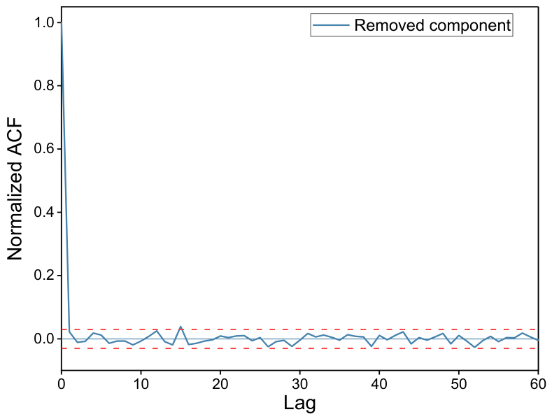
To verify the randomness of the removed component, the normalized Autocorrelation Function (ACF) is employed to quantify its temporal correlation. For a time series x_t, the normalized ACF at lag h is defined as

$$\rho (h)={\displaystyle \frac{{\displaystyle \sum _{t=1}^{N-h}(x_t-\overline{x})}(x_{t+h}-\overline{x})}{{\displaystyle \sum _{t=1}^N{(x_t-\overline{x})}^2}}}$$

(15)

where N is the sequence length and $\overline{x}$ is the mean. For an uncorrelated white-noise sequence, the sample ACF at nonzero lags is expected to fluctuate around zero; an approximate pointwise 95% reference interval is $\pm 1.96/\sqrt{N}$.

3. Combined Forecasting Model

3.1. Improved Whale Optimization Algorithm

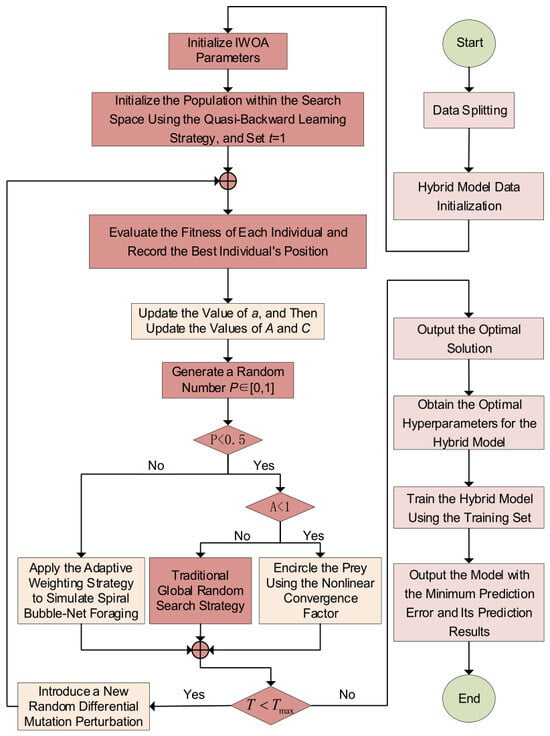
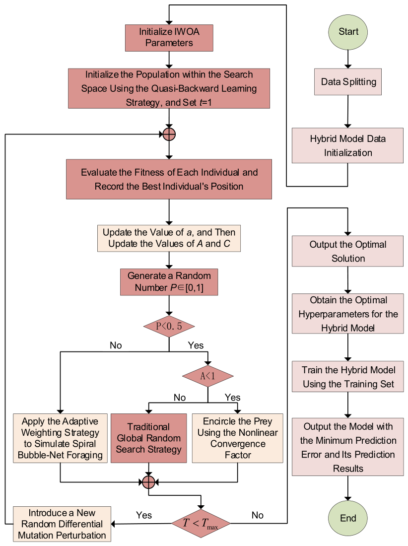
The IWOA is an improved version of the traditional WOA [24], and its workflow is illustrated in Figure 2.

Figure 2. Flowchart of IWOA.

3.1.1. Quasi-Opposition-Based Learning and Nonlinear Convergence Factor Strategies

The IWOA introduces a quasi-backward learning strategy during initialization to enhance the diversity and distribution of the initial population. The position of the i-th whale in the d-dimensional search space is represented as follows:

X_i = (x_i,1,x_i,2,…,x_i,d),x_i,j ∈ [a_i,j,b_i,j]

(16)

where a_i,j and b_i,j denote the lower and upper bounds of the j-th dimension, respectively. The corresponding quasi-backward solution x_i,j is expressed as follows:

$${\widehat{x}}_{i,j}=a_{i,j}+b_{i,j}-\mathrm{r}\cdot x_{i,j}$$

(17)

where r ∈ (0, 1) denotes a random coefficient.

During initialization, N randomly generated individuals are combined with N quasi-backward solutions generated through quasi-backward learning, yielding 2N candidate individuals. A maximum-diversity selection mechanism is then employed to select N individuals with higher population diversity to form the initial population. This strategy improves the diversity of the initial population while providing more favorable conditions for subsequent global exploration.

To enhance the algorithm’s global exploration capability during early iterations, a nonlinear convergence factor is introduced. The convergence factor is defined as follows:

$$a=2-2\sin \left(\mu {\displaystyle \frac{t}{t_{\max }}}\pi +\phi \right)$$

(18)

where t denotes the current iteration number; t_max denotes the maximum number of iterations; μ denotes the adjustment coefficient; and φ denotes the nonlinear control parameter.

3.1.2. Adaptive Weighting and Random Differential Mutation Strategies

To alleviate the algorithm’s tendency to become trapped in local optima, an adaptive weighting strategy and a random differential mutation strategy are introduced. During the encircling or spiral-updating phase, each whale performs two position updates. The first update is performed according to the adaptive weighting strategy, followed by a second update using the random differential mutation strategy. The position with the better fitness is selected as the final updated position, thereby enhancing the algorithm’s ability to escape local optima.

The adaptive weighting strategy is formulated as follows:

$$\omega =1-{\displaystyle \frac{e^{\frac{t}{\mathit{tmax}}}-1}{e-1}}$$

(19)

X(t + 1) = ω ⋅ X_p(t) + D ⋅ e^bl ⋅ cos(2πl)

(20)

The random differential mutation strategy is formulated as follows:

X(t + 1) = r₁(X_p(t) − X(t)) + r₂(X_r(t) − X(t))

(21)

where r₁ and r₂ denote random numbers uniformly distributed over the interval [0, 1]; X_p denotes the position of the best whale individual in the population; and X_r denotes the position of a randomly selected whale individual from the population.

3.2. TimeMixer

TimeMixer is a multiscale time series forecasting model based on a mixing architecture. It first decomposes the original time series into seasonal and trend components through time series decomposition and employs two core modules: Past Decomposable Mixing (PDM) and Future Multipredictor Mixing (FMM). The PDM module performs multiscale decomposition and mixing of historical time series during the encoding stage, while the FMM module generates multistep forecasts during the decoding stage. Through the interaction of these two modules, TimeMixer captures local variations and long-term trends across different time scales [25].

3.2.1. Multiscale Averaging and Pooling

Multiscale averaging and pooling produce time series views at different resolutions by downsampling the input sequence. Different pooling windows are employed to progressively compress the sequence, generating a set of representations ranging from fine to coarse scales. The fine-scale representations preserve local dynamic variations, whereas the coarse-scale representations highlight long-term trends. This multiscale structure enables the model to capture both local details and global trends, providing a foundation for subsequent seasonal-trend decomposition and cross-scale mixing, thereby enhancing its ability to model temporal dependencies across different scales.

3.2.2. PDM

PDM is the core module of TimeMixer for processing historical time series. It aims to enhance temporal feature representations and extract informative patterns from historical data through decomposable multiscale mixing. At each level l, PDM first performs seasonal-trend decomposition on the time series at each scale:

$$s_m^l,t_m^l=\mathrm{SeriesDecomp}(x_m^l),m\in \{0,\dots ,M\}$$

(22)

where $x_m^l$ denotes the input sequence at the m-th scale of the l-th layer; $s_m^l$ and $t_m^l$ denote the corresponding seasonal and trend components, respectively; m denotes the scale index; 0 denotes the original finest scale; M denotes the coarsest scale after downsampling; and SeriesDecomp() denotes the time series decomposition operation.

After decomposition, PDM applies bottom-up mixing to the seasonal components and top-down mixing to the trend components. Specifically, bottom-up mixing progressively aggregates fine-scale seasonal information to supplement the local details that may be lost in coarse-scale representations, whereas top-down mixing progressively propagates coarse-scale trend information to guide fine-scale trend modeling and maintain overall trend consistency. The resulting seasonal and trend components are then combined and passed through a nonlinear transformation in the feedforward layer. A residual connection is then added using the output x^l−1 of the previous layer, yielding the output of the l-th PDM layer as follows:

$$x^l=x^{l-1}+\mathrm{FeedForward}\left(\mathrm{S}\text{-}\mathrm{Mix}\left({\{s_m^l\}}_{m=0}^M\right)+\mathrm{T}\text{-}\mathrm{Mix}\left({\{t_m^l\}}_{m=0}^M\right)\right)$$

(23)

where x^l denotes the output of the l-th PDM layer; x^l−1 denotes the output of the previous PDM layer; S-Mix() and T-Mix() denote the bottom-up mixing of seasonal components and the top-down mixing of trend components, respectively; and FeedForward() denotes the feedforward layer.

3.2.3. FMM

FMM is the decoding module of TimeMixer and maps the multiscale historical features extracted by PDM to future forecasts. For each scale, FMM employs an independent linear predictor to process the corresponding sequence and generate multistep forecasts. Fine-scale forecasts capture ultra-short-term and high-frequency fluctuations, whereas coarse-scale forecasts reflect long-term and low-frequency trends. This multiscale forecasting strategy enables the model to characterize temporal patterns at different resolutions, providing rich forecasting information at multiple resolutions for subsequent adaptive fusion. The FMM module is formulated as follows:

$${\widehat{x}}_m={\mathrm{Predictor}}_m(x_m^l),m\{0,\cdots ,M\}$$

(24)

$$\widehat{x}={\displaystyle \sum _{m=0}^M{\widehat{x}}_m}$$

(25)

where Predictor_m denotes the predictor for the sequence at the m-th scale; ${\widehat{x}}_m$ denotes the forecasting result for the sequence at the m-th scale; and $\widehat{x}$ denotes the final forecasting result.

3.3. Mamba

Mamba is a sequence modeling framework based on the Selective State Space Model (SSM) [26]. Its core formulation is as follows:

$$h_t=\overline{A}(u_t)h_{t-1}+\overline{B}(u_t)u_t$$

(26)

y_t = C(u_t)h_t

(27)

where u_t denotes the current input; h_t denotes the hidden state; $\overline{A}(u_t)$, $\overline{B}(u_t)$ and C(u_t) are time-varying parameters that are dynamically generated from the input u_t through linear projection and discretization, rather than being fixed constants as in traditional state-space models. This selective mechanism enables Mamba to dynamically determine which information should be retained or discarded based on the current input, thereby preserving relevant long-term dependencies during periods of relatively stable wind power variation while responding effectively to sudden fluctuations.

For a seasonal time series S ∈ R^L, Mamba first projects the input sequence into a D-dimensional feature space through a linear layer and feeds the resulting features into an encoder composed of N stacked Mamba blocks. Each Mamba block consists of a one-dimensional convolution, a selective SSM, and residual connections, producing the output feature H^Mamba ∈ R^L×D. The feature $h_{\mathrm{L}}^{\mathrm{Mamba}}$ at the last time step is subsequently passed through a fully connected forecasting head to obtain the predicted seasonal component:

$${\widehat{Y}}_{\mathrm{s}}^{\mathrm{Mamba}}=W_{\mathrm{pred}}{h}_{\mathrm{L}}^{\mathrm{Mamba}}+b_{\mathrm{pred}}$$

(28)

where ${\widehat{Y}}_{\mathrm{s}}^{\mathrm{Mamba}}$ denotes the seasonal component forecast produced by Mamba; W_pred denotes the weight matrix; and b_pred denotes the bias term. Mamba’s linear recurrent structure has a computational complexity of O(L), enabling efficient modeling of long-term dependencies in wind power time series and complementing the TimeMixer branch.

3.4. TimeMixer-Mamba

TimeMixer-Mamba adopts a parallel dual-branch architecture for forecasting each IMF component. For the k-th IMF, the historical IMF sequence and the selected meteorological variables are concatenated along the feature dimension to form the input tensor X ∈ ℝ^B×L×D, where B, L, and D denote the batch size, input sequence length, and number of input variables, respectively. A linear projection maps these input features into a D-model-dimensional latent space, yielding $Z\in {ℝ}^{B\times L\times D_{\mathrm{model}}}$.

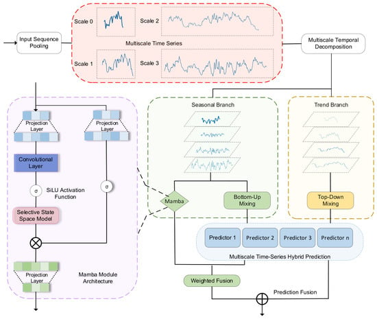
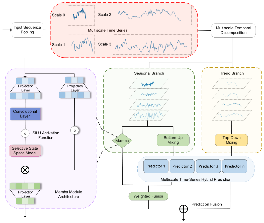
The shared input is first linearly projected into the latent feature space. In the TimeMixer branch, temporal downsampling is performed to construct multiple temporal scales. For the s-th scale, the representation is denoted as $Z^{(s)}\in {ℝ}^{B\times L_s\times D_{\mathrm{model}}}$, where L_s represents the corresponding temporal resolution. The feature dimension remains D_model across different scales. After multiscale temporal mixing, the representations are aligned and fused to obtain the TimeMixer representation. In parallel, the seasonal sequence derived from the shared input is supplied to the Mamba branch to capture temporal dependencies for ultra-short-term forecasting. The overall architecture of the proposed TimeMixer-Mamba model is illustrated in Figure 3.

Figure 3. TimeMixer-Mamba model.

To adaptively combine the two branch outputs, let the overall IMF forecast produced by the TimeMixer branch be denoted as ${\widehat{Y}}_s^{\mathrm{TM}}$, and let the seasonal forecast produced by the Mamba branch be denoted as ${\widehat{Y}}_{\mathrm{s}}^{\mathrm{Mamba}}$. First, the global context vectors C_TM ∈ R^D and C_Mamba ∈ R^D are extracted from the two branches, respectively. These vectors are then concatenated and fed into a two-layer gated network:

c = [c_TM;c_Mamba]

(29)

u = ReLU(W₁c + b₁)

(30)

λ=σ(W₂u+b₂)

(31)

where c denotes the concatenated input vector; W₁ and W₂ denote the weight matrices of the first and second layers, respectively; b₁ and b₂ denote the bias terms of the first and second layers, respectively; u denotes the hidden-layer output; ReLU() and σ denote the activation functions of the first and second layers, respectively; and λ ∈ R^H denotes the final output fusion weight vector.

The final IMF forecast is expressed as follows:

$${\widehat{Y}}_s=\lambda \odot {\widehat{Y}}_s^{\mathit{TM}}+(1-\lambda )\odot {\widehat{Y}}_s^{\mathit{Mamba}}$$

(32)

The fusion weight λ varies dynamically with the current input, allowing the model to adjust the relative contributions of the overall TimeMixer forecast and the Mamba seasonal forecast at each forecasting step. The TimeMixer branch provides the overall prediction after multiscale seasonal-trend modeling, whereas the Mamba branch provides additional information from the seasonal sequence, especially for abrupt and ultra-short-term fluctuations. The gated fusion therefore produces the final forecast of the corresponding IMF component directly. The forecasts of all IMF components are then summed to reconstruct the final wind power forecast.

4. Overall Model Workflow

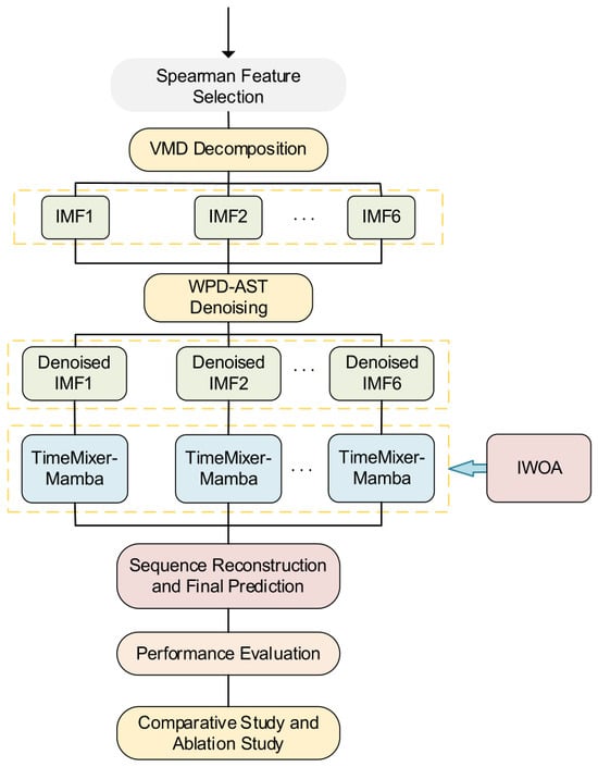
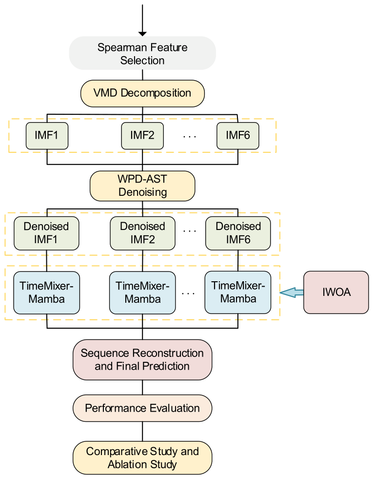
To improve the accuracy of wind power forecasting, this study proposes an ultra-short-term wind power forecasting model based on adaptive selective denoising and TimeMixer-Mamba. The overall forecasting framework is illustrated in Figure 4. To avoid information leakage, all time-dependent preprocessing operations follow a strictly causal rolling-window scheme, in which only observations available up to each forecasting origin t are used. The specific forecasting steps are as follows:

Figure 4. Overall Forecasting Framework of the Proposed Method.

Step 1: The dataset is chronologically divided into training, validation, and testing sets without random shuffling. Spearman’s rank correlation coefficient is calculated using the training set to analyze the correlations between meteorological variables and wind power. With TimeMixer-Mamba as the baseline model and validation-set RMSE as the evaluation metric, the optimal feature subset is determined and then fixed for the final testing phase. The testing set is not used for feature selection or hyperparameter optimization.

Step 2: During validation and testing, a rolling window containing only historical observations up to each forecasting origin *t* is constructed. VMD is performed within each window to obtain multiple IMF components with different temporal-scale characteristics. Correlation coefficients and sample entropy are then used to construct a composite noise score for adaptively identifying high-noise IMFs. High-noise IMFs are selectively denoised using WPD-AST, whereas low-noise IMFs are retained. Before the rolling-window decomposition, the VMD parameters are optimized using IWOA based solely on the training data, with the average permutation entropy of the resulting IMF components adopted as the objective function. The optimal number of modes and penalty factor are determined accordingly, and the optimized VMD parameters are then fixed during validation and testing. The latest denoised observations are subsequently used as inputs to TimeMixer-Mamba.

Step 3: During training, a TimeMixer-Mamba model is constructed for each IMF component, and IWOA is employed to optimize the key hyperparameters using the training and validation sets. The optimized hyperparameters are fixed during testing. At each forecasting origin, the latest denoised observations of each IMF are fed into the corresponding model to predict the IMF value at the next time step t + 1.

Step 4: The predicted IMF values are superimposed and reconstructed to obtain the final wind power forecast. Steps 2–4 are repeated chronologically over the validation and testing periods until the evaluation is completed. Finally, the proposed model is compared with other forecasting models to evaluate its forecasting performance.

Throughout the rolling process, VMD, WPD-AST denoising, noise scoring, and model input construction use only observations available up to the corresponding forecasting origin. Feature screening uses training-set correlations, and the final subset is selected using validation-set RMSE; the selected subset remains fixed during testing. Similarly, periodic VMD parameter updates use only historical observations available at the corresponding update time. Therefore, the entire preprocessing and forecasting procedure maintains strict temporal causality without introducing future information.

5. Case Study and Experimental Results

A wind power dataset collected from a wind farm in Gansu, China, from 1 January 2019 to 1 January 2020, is used for simulation validation. The dataset covers multiple seasons and is divided chronologically to avoid temporal data leakage. The data are sampled at 15-min intervals and divided into training, validation, and test sets at a ratio of 6:2:2, respectively. A sliding time window is employed to construct supervised learning samples, with the multivariate features from the past 96 time steps used as model inputs to forecast the wind power at the next time step. All models are implemented in the PyTorch 2.3.1 environment. The experimental hardware consists of an Intel Core i5-12700F processor, an NVIDIA RTX 4060 GPU with 8 GB of memory, and 16 GB of RAM.

5.1. Evaluation Metrics

To quantify the performance of the different forecasting methods, this study employs three commonly used metrics: root mean squared error (RMSE), mean absolute error (MAE), and coefficient of determination (R²). The corresponding formulas are given as follows:

$$\mathrm{RMSE}=\sqrt{{\displaystyle \frac{1}{n}}{\displaystyle \sum _{k=1}^n{(y_k-{y_k}^{\prime })}^2}}$$

(33)

$$\mathrm{MAE}={\displaystyle \frac{1}{n}}{\displaystyle \sum _{k=1}^n|}{y}_k-{y_k}^{\prime }|$$

(34)

$$R^2=1-{\displaystyle \frac{{\displaystyle \sum _{k=1}^n{(y_k-{y_k}^{\prime })}^2}}{{\displaystyle \sum _{k=1}^n{(y_k-\overline{y})}^2}}}$$

(35)

where y_k denotes the actual wind power value; y_k′ denotes the predicted wind power value; $\overline{y}$ denotes the mean wind power value; and n denotes the number of test samples.

5.2. Data Analysis and Preprocessing

5.2.1. Feature Selection

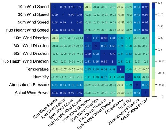
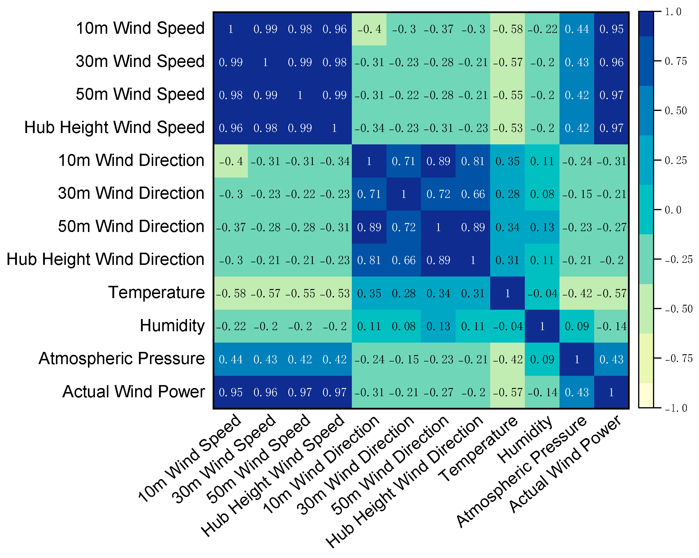
To analyze the relationships between wind power output and meteorological variables, this study employs the Spearman correlation coefficient P to quantify the correlations between the meteorological variables and wind power output. The selected meteorological variables include wind speed and wind direction measured at different heights (10 m, 30 m, 50 m, and hub height), as well as temperature, humidity, and atmospheric pressure. Figure 5 presents the correlations between the meteorological variables and wind power output.

Figure 5. Spearman Correlation Coefficient Matrix.

The results indicate that wind power output is positively correlated with wind speed and atmospheric pressure, whereas it is negatively correlated with wind direction, temperature, and humidity. In particular, wind speed measured at different heights exhibits a strong correlation with wind power output. Therefore, wind speed is retained as a representative feature, while features with relatively weak correlations with power output, including wind direction at 30 m, 50 m, and hub height and humidity, are excluded to reduce interference from redundant information. Although wind direction and atmospheric pressure measured at 10 m, as well as temperature, exhibit relatively weak correlations with wind power output, these variables may still contain complementary information. Accordingly, these features are retained after the initial screening and are further evaluated using the TimeMixer-Mamba model with RMSE as the evaluation metric to determine the optimal feature subset.

For further feature selection, TimeMixer-Mamba serves as the forecasting model, and RMSE serves as the evaluation metric. The feature selection process is performed iteratively. At each iteration, one feature is removed from the current feature set, and the TimeMixer-Mamba model is retrained using the remaining features to obtain the corresponding forecasting results. This process is repeated until all candidate feature subsets have been systematically evaluated. The optimal feature subset is then determined based on the RMSE, with a lower RMSE indicating better forecasting performance. The corresponding forecasting results are presented in Table 2.

Table 2. RMSE variation with iterative feature removal on the VMD–WPD-AST processed dataset without IWOA optimization.

Removed Features	RMSE
None	2.6127
10m Wind Direction	2.2882
10m Wind Direction, Atmospheric Pressure	2.0142
10m Wind Direction, Atmospheric Pressure, Temperature	2.2468
10m Wind Direction, Atmospheric Pressure, Temperature, 10m Wind Speed	2.5567
10m Wind Direction, Atmospheric Pressure, Temperature, 10m Wind Speed, 30m Wind Speed	2.7041

As shown in Table 2, using the VMD–WPD-AST processed dataset without IWOA optimization, the RMSE reached a minimum of 2.0142 after the 10 m wind direction and atmospheric pressure were removed, indicating the best forecasting performance among the evaluated feature subsets. Further feature removal resulted in degraded forecasting performance. Accordingly, wind speed at 10 m, 30 m, 50 m, and hub height, together with temperature, formed the best-performing subset among those evaluated.

5.2.2. Data Decomposition and Denoising

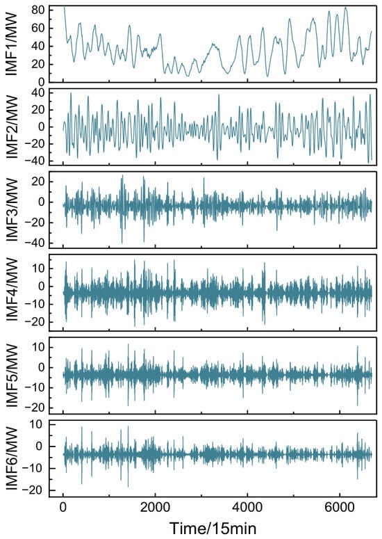
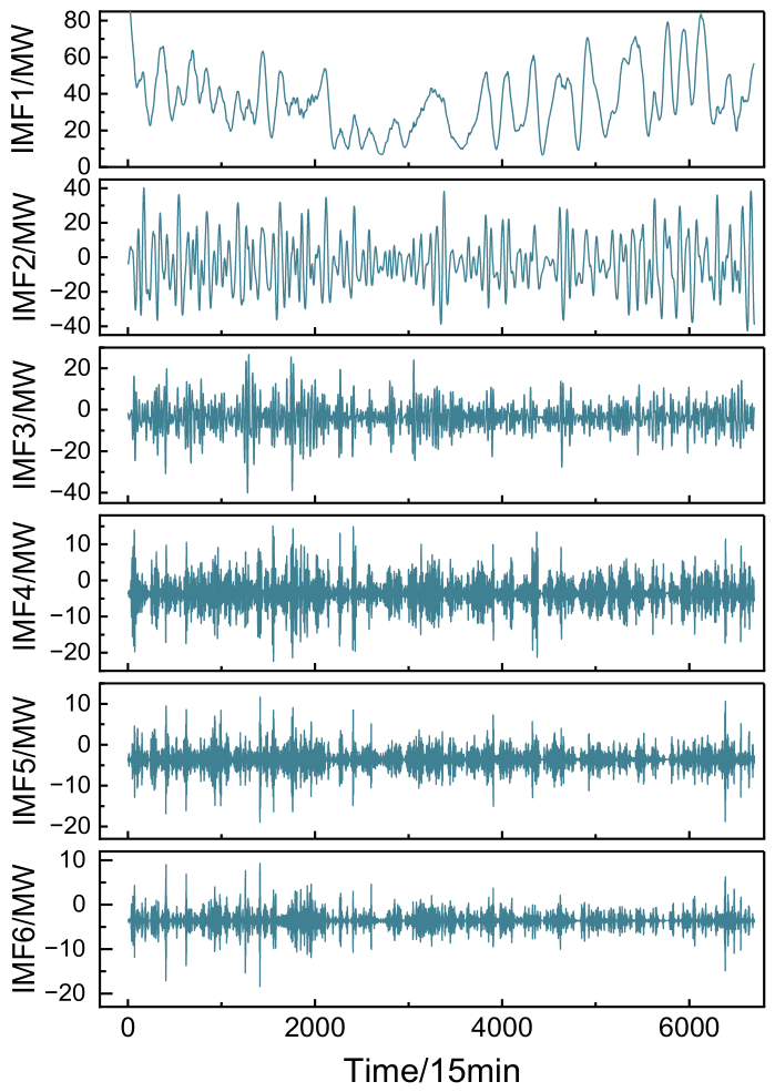
The number of decomposition modes, K, and the penalty factor, α, are key parameters affecting VMD performance. An excessively small K may result in insufficient decomposition and residual modal aliasing, whereas an excessively large K may introduce spurious components and increase computational redundancy. In this study, the VMD hyperparameters, including the number of modes K and the penalty factor, are first optimized using IWOA based solely on the training data. The optimized parameters are then fixed and used for VMD within each rolling historical window during validation and testing. The average permutation entropy of the IMF components is used as the objective function, and IWOA is employed to optimize K and α, with a population size of 25 and a maximum of 100 iterations. The optimization results show that the average permutation entropy reaches its minimum when K = 6 and α = 1140. Therefore, K = 6 and α = 1140 are selected as the optimal VMD parameters. The VMD results are presented in Figure 6.

Figure 6. VMD Results.

As shown in Figure 6, the oscillation frequency gradually increases from IMF1 to IMF6, while the corresponding time scale decreases. Among these components, IMF1 exhibits relatively smooth variations and primarily captures the low-frequency fluctuations of wind power output. IMF2 shows more pronounced low-to-medium-frequency periodic fluctuations. IMF3 and IMF4 exhibit stronger medium-to-high-frequency oscillations, reflecting the dynamic variations in the wind power time series at shorter time scales. In contrast, IMF5 and IMF6 exhibit more intense high-frequency fluctuations accompanied by occasional local abrupt changes. These results demonstrate that VMD effectively decomposes the original wind power time series into components with distinct frequency characteristics and time scales, thereby reducing coupling among different temporal patterns and providing a more suitable representation for subsequent noise identification and forecasting.

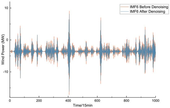
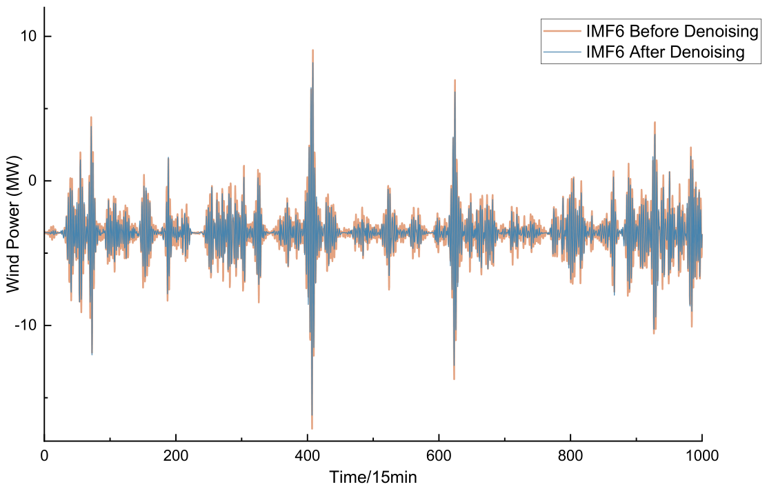
Subsequently, a comprehensive noise score is calculated for each IMF based on the correlation coefficient and sample entropy, enabling the adaptive identification of high-noise components. The identified high-noise IMFs are then selectively denoised using WPD-AST, whereas the low-noise IMFs are retained without further processing. Using IMF6 as an example, Figure 7 compares the component before and after denoising.

Figure 7. Comparison of IMF6 Before and After Denoising.

As shown in Figure 7, the raw IMF6 sequence exhibits pronounced high-frequency oscillations, with its amplitude fluctuating frequently between approximately −15 MW and 10 MW. After WPD-AST processing, the sequence becomes substantially smoother, with high-frequency random noise effectively suppressed while the main fluctuation patterns are preserved.

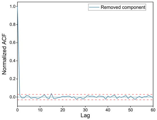
To verify that the removed component is predominantly noise rather than ramps, periodic fluctuations, or transient events, a statistical analysis was conducted, as shown in Figure 8. The normalized ACF remains close to zero at most nonzero lags and shows no evident periodic oscillations or slowly decaying tails, indicating weak global linear temporal correlation and noise-dominated behavior. To further examine whether transient events were preserved, the Pearson correlation coefficient between the original and denoised signals was calculated over the identified transient period. The coefficient exceeds 0.9, demonstrating that the denoised signal closely preserves the transient waveform and that the transient event was not mistakenly removed as noise.

Figure 8. Normalized ACF of the removed component.

5.3. Experimental Results and Analysis

5.3.1. IWOA-Based Hyperparameter Optimization and Convergence Analysis

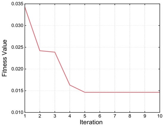
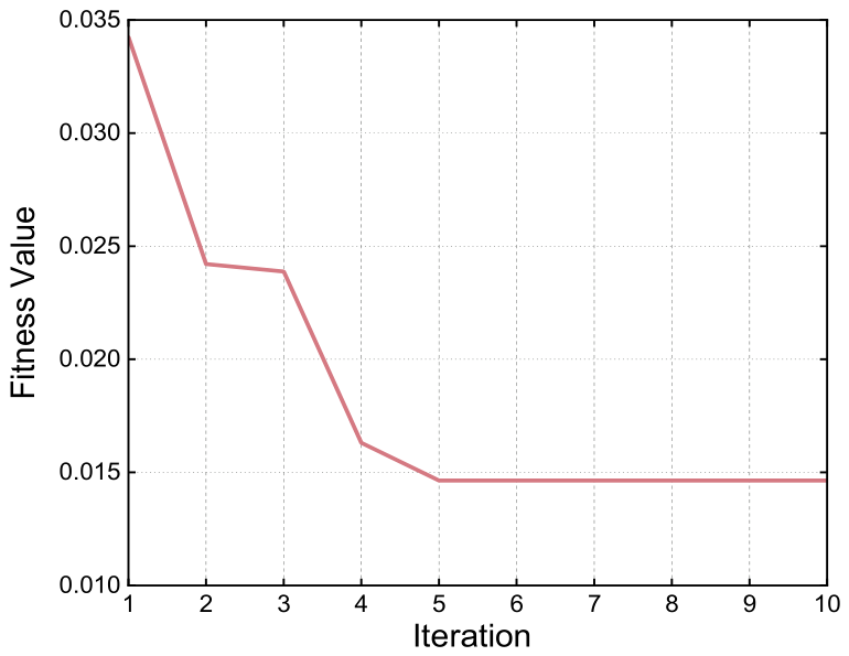
To obtain an appropriate combination of hyperparameters for the TimeMixer-Mamba model, IWOA was employed to optimize the key model hyperparameters. The prediction error on the validation set was used as the fitness function, and the positions of the whale individuals were iteratively updated to search for an optimal solution in the hyperparameter space. Taking the IMF6 component obtained from the original wind power sequence after VMD as an example, the IWOA fitness curve is presented in Figure 9.

Figure 9. Fitness Curve of IWOA.

As shown in Figure 9, the fitness value decreases markedly during the early optimization stage, indicating that IWOA rapidly searches for suitable hyperparameter combinations within the specified search space. As the number of iterations increases, the fitness value gradually stabilizes, with substantially smaller fluctuations in the later stage, indicating progressive convergence of the optimization process. After reaching a stable state, the best fitness value remains nearly unchanged, suggesting that a stable hyperparameter combination has been identified within the specified search range. These results indicate that IWOA can effectively optimize the key hyperparameters of TimeMixer-Mamba and provide an optimized configuration for the subsequent forecasting experiments.

Based on the optimization results, the optimal hyperparameter configuration for each IMF was selected according to its best validation-set performance and used to train the corresponding IMF-specific TimeMixer-Mamba model. Thus, six independent TimeMixer-Mamba models were trained separately for the six IMFs. For illustration, the search ranges and optimal hyperparameter values obtained for IMF6 are presented in Table 3. The optimization procedure was conducted independently for each IMF to account for their different temporal characteristics.

Table 3. IWOA-based hyperparameter optimization results for IMF6.

Optimization Parameters	Search Range	Optimal Value
dropout	[0.01, 0.4]	0.034
weight decay	[1 × 10−6, 1 × 10−3}	1.71 × 10−5
d_model	{32, 64, 128}	64
d_layers	{1, 2, 3}	2
d_state	{8, 16, 32}	16
learning rate	[1 × 10−5, 1 × 10−2]	0.0012

To ensure a fair comparison, IWOA was used to optimize the key hyperparameters of each model based on the validation-set RMSE. Only the most influential hyperparameters were included to balance optimization effectiveness and computational cost. The optimized hyperparameters are summarized in Table 4.

Table 4. Hyperparameter search spaces for the compared models.

Model	Hyperparameters Optimized by IWOA
BiLSTM	Hidden dimension; LSTM layers; dropout; learning rate
Transformer	d_model; nhead; encoder layers; dropout; learning rate
Mamba	d_model; d_state; d_conv; expand; Mamba layers; dropout
TimeMixer	d_model; d_ff; mixing blocks; d_layers; Learning rate
CNN-LSTM	Conv1D filters; kernel size; LSTM hidden units; LSTM layers; dropout
GRU-Attention	GRU hidden units; GRU layers; attention units; attention heads; dropout
CNN-Transformer	Conv1D filters; kernel size; d_model; encoder layers; dropout
Transformer-LSTM	d_model; nhead; encoder layers; LSTM hidden units; learning rate
TimeMixer-Mamba	weight decay; d_model; d_layers; d-state; learning rate; dropout
BiLSTM	Hidden dimension; LSTM layers; dropout; learning rate
Transformer	d_model; nhead; encoder layers; dropout; learning rate
Mamba	d_model; d_state; d_conv; expand; Mamba layers; dropout

5.3.2. Comparison of Different Forecasting Models

To verify the predictive effectiveness of the proposed model, the model is compared with conventional single models and hybrid models. The single models include ① BiLSTM, ② Transformer, ③ Mamba, and ④ TimeMixer, while the hybrid models include ⑤ CNN-LSTM, ⑥ GRU-Attention, ⑦ CNN-Transformer, and ⑧ Transformer-LSTM. All forecasting models are provided with the same input data after feature selection, comprehensive denoising, and VMD. For models of the same type, the relevant architectural and training settings were kept consistent to minimize the influence of parameter differences on the comparison results. For all models, the input window length was set to 96, and the maximum number of training epochs was set to 100. The key model-specific hyperparameters are listed in Table 5.

Table 5. Key hyperparameter settings of the compared models.

Model	Key Hyperparameter Settings
BiLSTM	Hidden dimension = 64; LSTM layers = 2; dropout = 0.1; learning rate = 0.001; batch size = 32
Transformer	d_model = 64; nhead = 4; encoder layers = 4; feedforward dimension = 256; dropout = 0.01; learning rate = 0.001; weight decay = 1 × 10−4; batch size = 32
Mamba	d_model = 64; d_state = 16; d_conv = 4; expand = 2; Mamba layers = 2; dropout = 0.1; learning rate = 0.001; weight decay = 1 × 10−4; batch size = 32
TimeMixer	d_model = 64; d_ff = 96; mixing blocks = 2; d_layers = 2; moving-average kernel = 25; top-k = 5; dropout = 0.1; learning rate = 0.001; weight decay = 1 × 10−4; batch size = 64
CNN-LSTM	Conv1D filters = 64; kernel size = 3; LSTM layers = 2; LSTM hidden units = 100; dropout = 0.2; learning rate = 0.001; batch size = 32
GRU-Attention	GRU layers = 2; GRU hidden units = 128; attention units = 50; attention heads = 4; dropout = 0.2; learning rate = 0.001; batch size = 32
CNN-Transformer	Conv1D filters = 32; kernel size = 3; CNN layers = 1; d_model = 64; nhead = 4; encoder layers = 2; feedforward dimension = 32; learning rate = 0.001; batch size = 32
Transformer-LSTM	d_model = 128; nhead = 8; encoder layers = 4; feedforward dimension = 256; dropout = 0.125; LSTM layers = 2; LSTM hidden units = 128; learning rate = 0.0014; weight decay = 1 × 10−4; batch size = 32
TimeMixer-Mamba	d_model = 64; d_ff = 96; mixing blocks = 2; d_layers = 2; moving-average kernel = 25; d_state = 16; d_conv = 4; expand = 2; TimeMixer layers = 2; dropout = 0.1; learning rate = 0.001; weight decay = 1 × 10−5; batch size = 32

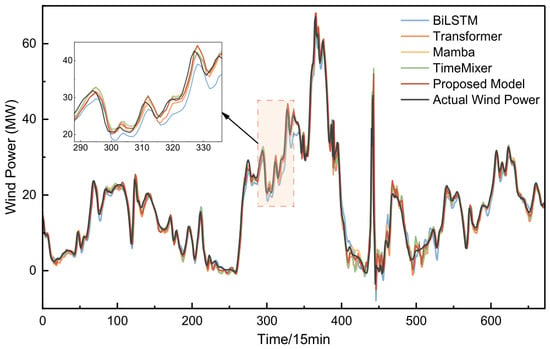
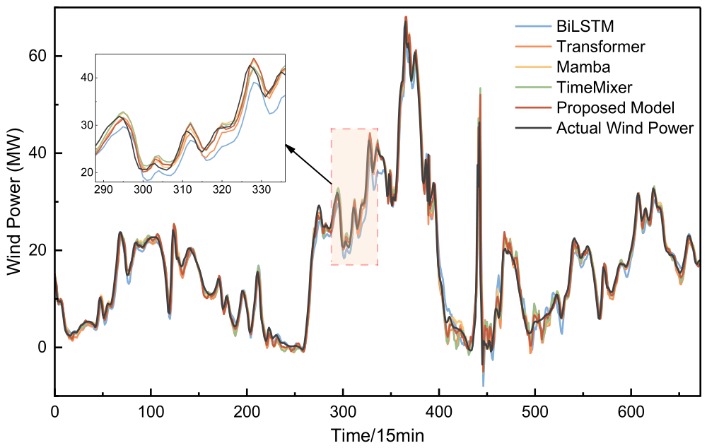
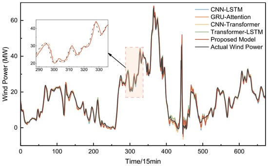
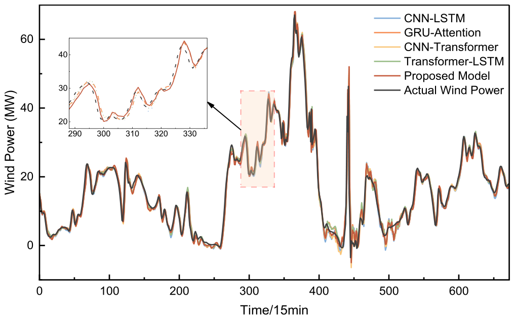
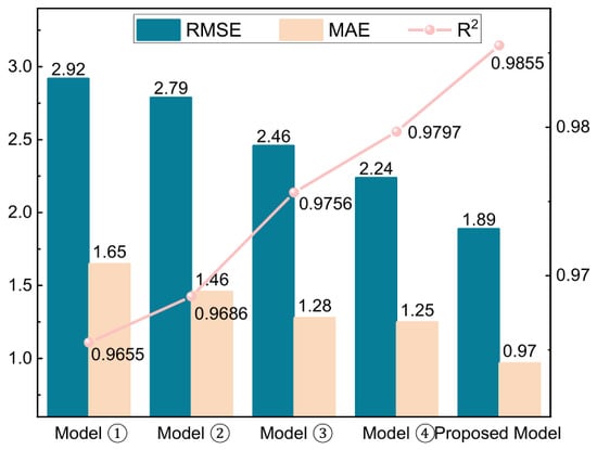
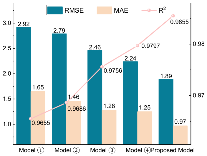
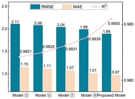
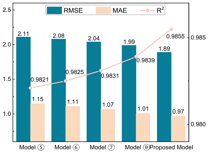
To facilitate a transparent and fair comparison, the first week of the validation set was pre-specified as the visualization window for Figure 10 and Figure 11. This period contains the first 672 forecasting points and was fixed in advance, independently of the forecasting results of any model. All compared models were evaluated over the same period, and their forecasting results together with the corresponding actual wind power values are presented in Figure 10 and Figure 11. Furthermore, the quantitative forecasting performance of each model was evaluated using the corresponding performance metrics, as presented in Figure 12 and Figure 13.

Figure 10. Comparison of forecasting results for single models.

Figure 11. Comparison of forecasting results for hybrid models.

Figure 12. Comparison of Forecasting Performance for single models.

Figure 13. Comparison of Forecasting Performance for hybrid models.

As shown in Figure 10, all single models capture the overall trend of wind power output reasonably well; however, noticeable deviations remain during periods of sharp power fluctuations. In particular, BiLSTM exhibits a clear lag around peaks and troughs. Although Transformer performs relatively well in capturing the overall trend, its ability to accurately characterize local fluctuations remains limited. In comparison, TimeMixer achieves a closer fit to the actual curve during relatively stable periods with less fluctuation in its forecasts, indicating that its multiscale decomposition and mixing mechanism can effectively capture temporal patterns and long-term trends at different time scales. Mamba, in contrast, demonstrates a faster response to abrupt changes in wind power, with relatively small forecasting errors around peak regions. This suggests that its selective state-space mechanism enhances its ability to adapt to rapidly varying input patterns, allowing it to better capture abrupt changes in nonstationary wind power time series. Overall, the results demonstrate that TimeMixer and Mamba exhibit complementary strengths in wind power forecasting, providing a reasonable basis for their integration into the proposed TimeMixer-Mamba hybrid model.

As shown in Figure 11, the hybrid models generally achieve a better overall fit than the single models and exhibit an improved ability to capture the nonlinear characteristics of wind power output. Specifically, CNN-LSTM employs convolutional layers to extract local features from the input sequence, but still exhibits some lag during periods of abrupt power increases. GRU-Attention introduces an attention mechanism to assign adaptive weights to key time steps, thereby reducing forecasting errors around peak regions compared with CNN-LSTM; however, its ability to consistently capture long-term trends remains limited. CNN-Transformer combines CNN’s local feature extraction capability with Transformer’s global dependency modeling capability, achieving a relatively good balance between stable and highly volatile periods, although it still tends to underestimate extreme peak values. As a dual-branch architecture, Transformer-LSTM further balances global trend modeling and local dynamic feature extraction, resulting in better overall forecasting performance than the other three hybrid models, although its tracking accuracy during periods of steep power declines remains limited. In comparison, the proposed TimeMixer-Mamba model achieves the best overall performance among the evaluated models. It maintains a low forecasting bias during relatively stable periods while accurately tracking actual power variations at key turning points, including abrupt increases and decreases, peaks, and troughs. These results further demonstrate the effectiveness of the proposed TimeMixer-Mamba model for ultra-short-term wind power forecasting.

As shown in Figure 12, among the single models, the proposed model achieves an RMSE of 1.89 and an MAE of 0.97, which are substantially lower than those of the other models, demonstrating its ability to reduce forecasting errors. Compared with TimeMixer, which achieves the best performance among the other single models, the proposed model reduces the RMSE and MAE by approximately 15.3% and 22.4%, respectively, while achieving an R² of 0.9855. These results indicate that the proposed model provides a more accurate fit to the actual wind power output and captures its variation patterns more precisely. The introduction of the Mamba module enhances TimeMixer’s ability to model long-range temporal dependencies, thereby improving its ability to characterize complex temporal variations in wind power.

As shown in Figure 13, among the hybrid models, although all hybrid models achieve improved forecasting accuracy compared with the single models, their overall performance remains inferior to that of the proposed model. Specifically, compared with Transformer-LSTM, which achieves the best performance among the hybrid models, the proposed model reduces the RMSE and MAE by approximately 5.2% and 4.0%, respectively, while achieving an R² of 0.9855. These results further demonstrate the performance advantage of the proposed TimeMixer-Mamba model over both conventional single models and hybrid models.

In summary, in comparisons with both single and hybrid models, the proposed model consistently achieves the best forecasting performance, demonstrating the effectiveness and superiority of the proposed TimeMixer-Mamba model for ultra-short-term wind power forecasting.

5.3.3. Ablation Study

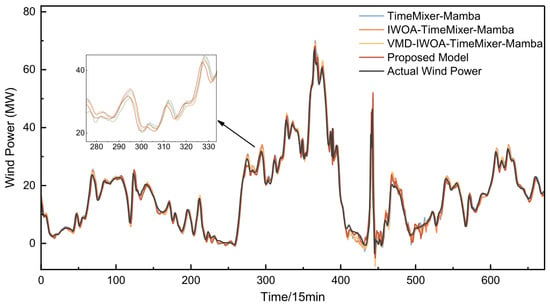
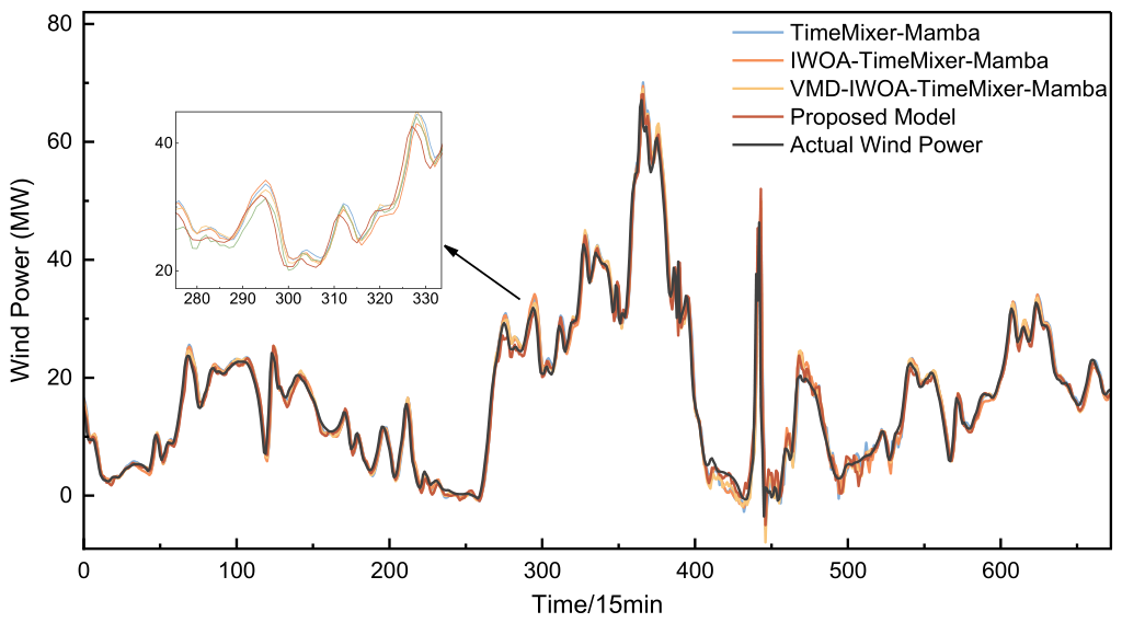
To verify the effectiveness of each module in the proposed model, an ablation study is conducted to systematically evaluate the contributions of different modules to forecasting performance. The wind power forecasting results are presented in Figure 14, while the corresponding evaluation metrics are summarized in Table 6.

Figure 14. Ablation Study Results.

Table 6. Performance Comparison of Ablation Models.

Forecasting Model	RMSE	MAE	R2
TimeMixer-Mamba	2.42	1.26	0.9764
IWOA-TimeMixer-Mamba	2.19	1.14	0.9805
VMD-IWOA-TimeMixer-Mamba	1.93	1.01	0.9849
VMD-WPD-AST-IWOA-TimeMixer-Mamba	1.89	0.97	0.9855

As shown in Figure 14 and Table 6, the overall forecasting performance improves progressively with the sequential introduction of the functional modules. The baseline TimeMixer-Mamba model exhibits some capability for time series modeling, but its forecasting errors remain relatively large. After IWOA is introduced to optimize the key hyperparameters, the model achieves a more appropriate parameter configuration, resulting in improved forecasting accuracy. Specifically, the RMSE and MAE decrease from 2.42 and 1.26 to 2.19 and 1.14, respectively, while R² increases to 0.9805. These results demonstrate that IWOA can effectively improve the hyperparameter configuration of TimeMixer-Mamba and enhance its forecasting accuracy, highlighting the value of intelligent optimization for hyperparameter tuning in deep learning models. With the further incorporation of VMD, the original wind power time series is decomposed adaptively into multiple IMF components with distinct frequency characteristics. The RMSE and MAE are further reduced to 1.93 and 1.01, respectively, while R² increases to 0.9849. This improvement indicates that VMD can effectively separate multiscale temporal patterns in the wind power signal, thereby reducing the difficulty of simultaneously modeling features at different temporal scales and further improving forecasting accuracy. Finally, the proposed comprehensive noise score based on the correlation coefficient and sample entropy is introduced together with the WPD-AST adaptive selective denoising strategy. The RMSE and MAE are further reduced to 1.89 and 0.97, respectively, while R² increases to 0.9855. These results indicate that selectively denoising high-noise IMFs can effectively suppress random noise while preserving key power fluctuation information, thereby further improving the forecasting performance of the proposed model.

As the functional modules are progressively incorporated, the overall forecasting performance improves accordingly, demonstrating the complementary contributions of the individual modules. Specifically, IWOA improves forecasting accuracy through more effective hyperparameter optimization; VMD reduces the nonstationarity of the original wind power sequence through multiscale decomposition; and WPD-AST adaptive selective denoising further improves data quality by suppressing noise while preserving useful fluctuation information. Overall, the ablation study demonstrates the soundness and effectiveness of the proposed module designs and their integration, with each module contributing to the final forecasting performance of the proposed model.

6. Conclusions

To improve the accuracy of ultra-short-term wind power forecasting, this study proposes a forecasting method based on adaptive selective denoising and TimeMixer-Mamba and systematically validates its effectiveness using real-world wind farm data. The main conclusions are as follows:

(1) For data preprocessing, an adaptive selective denoising method based on VMD-WPD-AST was developed. By selectively denoising high-noise IMF components, the proposed framework suppresses random noise while preserving key wind power fluctuation information, thereby providing higher-quality inputs for subsequent forecasting. In the ablation study, the inclusion of WPD-AST provided a moderate additional improvement, with RMSE decreasing from 1.93 to 1.89, MAE decreasing from 1.01 to 0.97, and R² increasing by 0.0006.

(2) For model construction and optimization, a TimeMixer-Mamba hybrid forecasting model was developed, in which the outputs of the two branches are adaptively fused through a gated network to integrate global trend modeling and local dynamic feature extraction. Furthermore, IWOA was employed to optimize the key hyperparameters of the model, contributing to improved forecasting performance in the evaluated case.

(3) The experimental results show that forecasting performance progressively improves with the sequential incorporation of the proposed functional modules, and the sequential ablation study supports incremental improvements in the evaluated configurations. Compared with the conventional single models and hybrid models, the proposed method achieves lower RMSE and MAE and higher R² for the single wind farm and 15-min forecasting horizon considered in this study. However, no probabilistic evaluation was performed, and the improvement provided by WPD-AST was moderate. Therefore, the conclusions are limited to the evaluated case, and no claims are made regarding statistical significance, repeated-run stability, runtime advantages, or multi-site generalization.

In summary, the proposed ultra-short-term wind power forecasting method improves point forecasting accuracy on a single wind farm dataset with a 15-min forecasting horizon. Future research will focus on model simplification, collaborative modeling across multiple wind farms, and uncertainty forecasting to further improve the engineering applicability and practical value of the proposed method.

References

- Li, T.; Ai, L.J.; Yang, Q.S.; Zhang, X.X.; Li, H.; Lu, D.W.; Shen, H.T. Short-term wind power prediction based on multiscale numerical simulation coupled with deep learning. Renew. Energy 2025, 246, 122951. [Google Scholar] [CrossRef] [Scilit]
- Yang, M.; Che, R.Q.; Yu, X.N.; Su, X. Dual NWP wind speed correction based on trend fusion and fluctuation clustering and its application in short-term wind power prediction. Energy 2024, 302, 131802. [Google Scholar] [CrossRef] [Scilit]
- Zhu, G.P.; Jia, W.Q.; Xing, Z.T.; Xiang, L.; Hu, A.J.; Hao, R.J. CMLLM: A novel cross-modal large language model for wind power forecasting. Energy Convers. Manag. 2025, 330, 119673. [Google Scholar] [CrossRef] [Scilit]
- Li, K.; Yuan, L.; Qian, F.; Song, L.; Wu, X.; Wang, L.; Dai, J.; Shen, L. Short-Term Load Forecasting for Electricity Spot Markets Across Different Seasons Based on a Hybrid VMD-LSTM-Random Forest Model. Energies 2025, 18, 6097. [Google Scholar] [CrossRef] [Scilit]
- Rayi, V.K.; Mishra, S.P.; Naik, J.; Dash, P.K. Adaptive VMD based optimized deep learning mixed kernel ELM autoencoder for single and multistep wind power forecasting. Energy 2022, 244, 122585. [Google Scholar] [CrossRef] [Scilit]
- Sun, X.; Han, B.; Song, Y.; Wang, Y.; Hou, E.; Wang, J.; Xu, Y. Short-Term Wind Power Forecasting Based on Dual-Optimized VMD-CNN-BiLSTM. Energies 2026, 19, 2317. [Google Scholar] [CrossRef] [Scilit]
- Yang, M.; Han, C.; Zhang, W. Short-term power prediction method for wind farm cluster based on deep graph clustering and feature reconstruction. Electr. Power Autom. Equip. 2025, 45, 53–59. [Google Scholar] [CrossRef]
- Chang, Y.; Yang, Z.; Pan, F.; Tang, Y.; Huang, W. Ultra-short-term Wind Power Prediction Based on CEEMDAN-PE-WPD and Multi-objective Optimization. Power Syst. Technol. 2023, 47, 5015–5026. [Google Scholar] [CrossRef]
- Liu, S.J.; Xu, T.; Du, X.Z.; Zhang, Y.C.; Wu, J.B. A hybrid deep learning model based on parallel architecture TCN-LSTM with Savitzky-Golay filter for wind power prediction. Energy Convers. Manag. 2024, 302, 118122. [Google Scholar] [CrossRef] [Scilit]
- Ahmadi, M.; Aly, H.; Khashei, M. Enhancing power grid stability with a hybrid framework for wind power forecasting: Integrating Kalman Filtering, Deep Residual Learning, and Bidirectional LSTM. Energy 2025, 334, 137752. [Google Scholar] [CrossRef] [Scilit]
- Yin, L.F.; Liu, Y.F. Bidirectional encoder representations from transformer fusion quantum dual-stage attention bidirectional gated recurrent unit and diffusion method for short-term wind power prediction. Eng. Appl. Artif. Intell. 2026, 169, 114095. [Google Scholar] [CrossRef] [Scilit]
- Jia, W.H.; Sun, J.; Guan, S.P. FPQ-iTransformer: A novel iTransformer-based model for accurate seawater salinity prediction. Environ. Model. Softw. 2025, 192, 106529. [Google Scholar] [CrossRef] [Scilit]
- Yang, F.; Zhang, J.Y. Medium and Short-Term Wind Power Forecasting Using LCNN-Mamba Model Based on Quadratic Decomposition. Sustainability 2026, 18, 7232. [Google Scholar] [CrossRef] [Scilit]
- Gong, M.J.; Wu, Z.H.; Zhang, F.; Sun, M.H.; Huang, J.B.; Tian, Y.; Xu, W. Adaptive multi-scale short term wind power forecasting framework based on TimeMixer and Mix-of-Experts. Electr. Power Syst. Res. 2026, 251, 112196. [Google Scholar] [CrossRef] [Scilit]
- Cai, Z.; Dai, S.; Ding, Q.; Zhang, J.L.; Xu, D.; Li, Y.X. Gray wolf optimization-based wind power load mid-long term forecasting algorithm. Comput. Electr. Eng. 2023, 109, 108769. [Google Scholar] [CrossRef] [Scilit]
- Lu, W.C.; Duan, J.D.; Wang, P.; Ma, W.T.; Fang, S. Short-term Wind Power Forecasting Using the Hybrid Model of Improved Variational Mode Decomposition and Maximum Mixture Correntropy Long Short-term Memory Neural Network. Int. J. Electr. Power Energy Syst. 2023, 144, 108552. [Google Scholar] [CrossRef] [Scilit]
- Liang, Y.; Zhang, D.Q.; Zhang, J.Z.; Hu, G. A state-of-the-art analysis on decomposition method for short-term wind speed forecasting using LSTM and a novel hybrid deep learning model. Energy 2024, 313, 133826. [Google Scholar] [CrossRef] [Scilit]
- Li, K.; Li, L.; Tang, J.; Dick, G.; Wickert, J.; Yu, H.; He, Q.M.; Dong, Z.N. Research on the PWV prediction model based on the ERA5-PWV calibration and WOA-RNN-BiLSTM-multihead-attention fusion algorithms. Atmos. Res. 2025, 325, 108238. [Google Scholar] [CrossRef] [Scilit]
- Bozorgi, S.M.; Yazdani, S. IWOA: An improved whale optimization algorithm for optimization problems. J. Comput. Des. Eng. 2019, 6, 243–259. [Google Scholar] [CrossRef] [Scilit]
- Su, Y.X.; Wang, Z.Y.; Dong, Z.C.; Hua, X.J.; Ye, T.; Song, Z.D.; Shao, Y. Frequency-aware ultra-short-term wind power forecasting using CEEMDAN-VMD-SE and Transformer-GRU networks. Energy 2025, 338, 138715. [Google Scholar] [CrossRef] [Scilit]
- Hou, L.X.; Wang, Q.Y.; Liu, D.Y. Real time prediction of ship motion based on iTransformer with EWT-SampEn data processing. Ocean Eng. 2025, 342, 122987. [Google Scholar] [CrossRef] [Scilit]
- Wu, Q.; Li, G.; Wang, X.; Luo, H.; Li, L.H.; Chen, Q.B.; Jing, X.R. Jamming recognition method based on wavelet packet decomposition and improved deep learning. Digit. Commun. Netw. 2025, 11, 1469–1478. [Google Scholar] [CrossRef] [Scilit]
- Nasiri, A.; Rahideh, A.; Agah, G.R.; Kia, S.H. Ball-Bearing Fault Detection of Squirrel-Cage Induction Motors Based on Single-Phase Stator Current Using Wavelet Packet Decomposition and Statistical Features. IEEE Trans. Energy Convers. 2025, 40, 1529–1537. [Google Scholar] [CrossRef] [Scilit]
- Han, X.S.; Shi, Y.; Tong, R.J.; Wang, S.T.; Zhang, Y. Research on short-term load forecasting of power system based on IWOA-KELM. Energy Rep. 2023, 9, 238–246. [Google Scholar] [CrossRef] [Scilit]
- Wang, S.; Wu, H.; Shi, X.; Hu, T.; Luo, H.; Ma, L.; Zhang, J.Y.; Zhou, J. TimeMixer: Decomposable Multiscale Mixing for Time Series Forecasting. arXiv 2024. [Google Scholar] [CrossRef] [Scilit]
- Gu, A.; Dao, T. Mamba: Linear-Time Sequence Modeling with Selective State Spaces. arXiv 2023. [Google Scholar] [CrossRef] [Scilit]
Disclaimer/Publisher’s Note: The statements, opinions and data contained in all publications are solely those of the individual author(s) and contributor(s) and not of MDPI and/or the editor(s). MDPI and/or the editor(s) disclaim responsibility for any injury to people or property resulting from any ideas, methods, instructions or products referred to in the content. |
© 2026 by the authors. Licensee MDPI, Basel, Switzerland. This article is an open access article distributed under the terms and conditions of the Creative Commons Attribution (CC BY) license.