


Abstract
Accurate photovoltaic (PV) power forecasting is becoming increasingly important for the secure and economical operation of renewable-rich power systems. However, conventional data-driven forecasting methods generally rely on sufficient site-specific historical observations, limiting their applicability to newly commissioned PV stations with severe data scarcity; meanwhile, forecasting performance is still predominantly evaluated using statistical error metrics, which cannot fully reflect its practical value in power system operation. To address these issues, this study develops a PV forecasting framework based on the pretrained time-series foundation model TimesFM, which exploits transferable temporal representations to enable zero-shot forecasting with limited target-site data. A lightweight residual quantile few-shot adaptation scheme is further introduced to learn station-specific forecasting deviations from limited historical observations while keeping the pretrained forecasting backbone fixed, thereby improving target-site adaptation and forecasting capability. In addition, a multi-dimensional power-system-operation-oriented evaluation framework is established to assess forecasting performance from economic, flexibility, regulation, and network-operation perspectives, together with different PV integration locations and installed capacities. Experimental results demonstrate that for the investigated CYT Station 1 case, the proposed method improves deterministic and probabilistic forecasting performance relative to zero-shot TimesFM and achieves substantial adaptation gains using limited target-site observations. The improved forecasts also reduce forecasting-induced operating costs and reserve requirements and yield system responses closer to those obtained with actual PV generation, confirming that forecasting improvements can be translated into measurable operational benefits.
1. Introduction
With the accelerating transition toward low-carbon power systems, photovoltaic (PV) generation has become one of the fastest-growing renewable energy resources worldwide [1,2]. The continuous expansion of PV has significantly reshaped both the operation and long-term planning of modern power systems, particularly as renewable penetration and associated uncertainties continue to increase [3]. Since PV output is inherently affected by solar irradiance, cloud movement, ambient temperature, and other meteorological factors, it exhibits strong intermittency, uncertainty, and temporal variability [4,5]. With increasing PV penetration, these characteristics impose growing challenges on power system operation, including economic dispatch, reserve allocation, and flexibility management [6,7]. Accurate PV power forecasting is therefore essential for secure and economical system operation, as reliable forecasts can improve renewable energy utilization, reduce unnecessary reserve deployment, and alleviate balancing pressure [8,9].
Existing PV forecasting approaches generally include physical, statistical, and data-driven methods [4,5]. Physical methods mainly rely on numerical weather prediction and physical descriptions of PV conversion processes [10], while statistical methods provide relatively simple and interpretable forecasting solutions but are limited in representing highly nonlinear PV generation patterns [11]. With the increasing availability of operational data, machine learning and deep learning approaches have become widely adopted for short-term PV forecasting because of their strong nonlinear representation capability [12,13]. More broadly, artificial intelligence is becoming increasingly embedded in the analysis and decision-making processes of electric energy systems [14]. Representative forecasting methods include recurrent neural networks, temporal convolutional networks, and Transformer-based architectures [12,15]. However, the performance of these models generally depends on sufficient historical observations from the target PV station [16]. This dependence becomes a major limitation for newly commissioned PV stations, where only limited historical data may be available before forecasting services are required for operational scheduling [17,18].
Recently, time-series foundation models (TSFMs) have provided a promising alternative for forecasting under limited-data conditions. Through large-scale pretraining on heterogeneous time-series datasets, TSFMs learn transferable temporal representations that enable zero-shot forecasting on previously unseen time series without task-specific retraining [19,20]. Among these models, TimesFM has demonstrated competitive forecasting performance across diverse benchmark datasets, indicating strong cross-domain generalization capability [20]. Such pretrained models therefore provide a potential solution for newly commissioned PV stations by reducing the dependence on large amounts of site-specific training data.
Nevertheless, directly applying pretrained TSFMs to PV forecasting still faces important challenges. Because foundation models are pretrained to capture general temporal patterns rather than the characteristics of a specific PV station, zero-shot forecasting performance may deteriorate when the target-site data distribution differs substantially from that encountered during pretraining. Recent studies have therefore explored lightweight and parameter-efficient adaptation of time-series foundation models for out-of-domain forecasting and online adaptation [21,22,23]. However, achieving effective station-specific adaptation remains difficult when only a very limited number of target-site observations are available. This motivates the development of lightweight few-shot adaptation strategies that can incorporate station-specific information while preserving the transferable forecasting capability of the pretrained backbone.
Despite recent progress, two issues remain insufficiently addressed. First, existing studies on data-scarce PV forecasting mainly focus on transfer learning, few-shot learning, or specialized prediction architectures [17,24], whereas lightweight adaptation methods specifically designed for pretrained TSFMs under extremely limited target-site data remain relatively underexplored [21,22,23]. Efficiently capturing station-specific characteristics without extensively updating the pretrained forecasting backbone therefore remains an important research problem. Second, PV forecasting models are still predominantly evaluated using statistical metrics such as MAE, RMSE, and MAPE [4,5,25]. Although these indicators quantify numerical forecasting errors, they cannot directly reveal how forecasting errors propagate into subsequent power system operation [26]. Recent studies have further demonstrated that degradation or manipulation of renewable energy forecasting can affect downstream operational decisions and introduce additional economic and system-level risks [27]. Since PV forecasts ultimately support scheduling, reserve allocation, balancing, and other operational decisions, improvements in statistical forecasting accuracy do not necessarily translate proportionally into operational benefits [8,28]. Therefore, a comprehensive evaluation framework is needed to connect forecasting performance with multi-dimensional power system operational consequences.
To address these issues, this paper develops a pretrained foundation model-based PV forecasting framework for data-scarce PV stations by integrating zero-shot time-series forecasting, lightweight residual few-shot adaptation, and power-system-operation-oriented performance evaluation. The main contributions are summarized as follows.
(1) A pretrained foundation model-based PV forecasting framework is proposed for newly commissioned PV stations with limited historical observations. Instead of training forecasting models from scratch, the proposed framework exploits the cross-domain temporal representation capability of TimesFM to perform zero-shot PV power forecasting, establishing a unified forecasting paradigm that effectively alleviates the dependence of conventional deep learning models on large target-site datasets.
(2) A lightweight residual quantile few-shot adaptation scheme is developed for pretrained foundation models under data-scarce PV scenarios. By keeping the pretrained TimesFM backbone fixed, the proposed scheme learns station-specific residual quantiles from limited historical observations and incorporates basic physical consistency constraints as feasibility safeguards, thereby improving target-site forecasting without requiring full-model parameter updating.
(3) A multi-dimensional power-system-operation-oriented evaluation framework for PV power forecasting is developed to bridge forecasting accuracy and practical operational value. By embedding different PV forecasting results into the IEEE 30-bus system, the proposed framework jointly evaluates operating cost, reserve requirement, generator ramping, voltage deviation, PV integration location sensitivity, and PV penetration sensitivity, thereby quantifying the system-level consequences of forecasting errors and the operational benefits brought by forecasting improvement.
The rest of this article organized as follows. Section 2 introduces the pretrained time-series foundation model-based PV forecasting framework. Section 3 presents the proposed few-shot adaptation strategy for data-scarce PV forecasting. Section 4 describes the multi-dimensional power-system-operation-oriented evaluation framework. Section 5 presents the case studies and discusses both forecasting and system-level evaluation results. Finally, Section 6 concludes the article and outlines potential directions for future research.
2. Pretrained Time-Series Foundation Model-Based PV Forecasting Framework
2.1. Overall Framework
The overall architecture of the proposed PV forecasting framework is illustrated in Figure 1. Different from conventional data-driven forecasting methods that require training forecasting models using a large amount of station-specific historical data, the proposed framework combines a pretrained TSFM with a lightweight few-shot adaptation strategy to achieve accurate forecasting for data-scarce PV stations. Furthermore, instead of evaluating forecasting performance solely using statistical error metrics, the proposed framework establishes a prediction-driven power-system evaluation process to quantify the operational value of forecasting improvement from the perspective of power system operation.
Figure 1.
Overall framework of the proposed pretrained foundation model-based PV forecasting and power-system-oriented evaluation methodology.
In Figure 1, solid arrows indicate the sequential information flow between the main forecasting stages, whereas dashed arrows indicate the linkage between the forecasting process and the prediction-driven power-system evaluation. As shown in Figure 1, the proposed framework consists of four sequential stages, namely data preprocessing, foundation forecasting, residual few-shot adaptation, and power-system-oriented evaluation. These four stages are closely connected and jointly form a complete forecasting-to-operation workflow.
In Stage I, historical PV power observations collected from the target station are first preprocessed through data cleansing, normalization, and sliding-window construction. The processed historical sequence is then transformed into a unified input representation suitable for the pretrained TSFM. Since all forecasting models share the same preprocessing procedure, the input consistency is guaranteed throughout subsequent experiments.
In Stage II, the standardized historical sequence is directly fed into the pretrained TimesFM foundation model to generate multi-step zero-shot forecasts without retraining the backbone model. Benefiting from large-scale pretraining on diverse time-series datasets, TimesFM provides transferable temporal representations and serves as a pretrained forecasting backbone for newly deployed PV stations with limited historical observations [20].
Although the pretrained model significantly alleviates the dependence on target-site historical data, systematic forecasting deviations may still exist because the statistical characteristics of the target station differ from those encountered during large-scale pretraining. Therefore, Stage III introduces a lightweight residual quantile adaptation scheme that learns station-specific forecasting discrepancies using a small amount of recent historical observations. Instead of modifying the foundation model itself, the RQA estimates residual quantiles between the zero-shot predictions and actual PV outputs and uses them to construct the adapted probabilistic forecasts. This design preserves the pretrained forecasting backbone while enabling station-specific adaptation under data-scarce conditions.
Finally, Stage IV evaluates the forecasting results from both prediction and power-system perspectives. Alongside conventional statistical metrics, including MAE and RMSE, the forecasting results are further embedded into the IEEE 30-bus system for sequential hourly AC-OPF evaluation. System-level operational indicators, including operating cost, reserve requirement, generator ramping, and voltage deviation, are subsequently calculated to quantify the practical operational value brought by forecasting improvement. In this way, the proposed framework establishes a complete bridge from PV forecasting to power-system operation, enabling comprehensive evaluation of forecasting algorithms beyond traditional prediction accuracy.
2.2. Pretrained Time-Series Foundation Model for Zero-Shot PV Forecasting
To overcome the strong dependence of conventional deep learning models on large amounts of target-station historical data, the proposed framework adopts a pretrained TSFM as the forecasting backbone. Unlike traditional supervised forecasting methods that require model retraining using station-specific observations, the pretrained foundation model directly performs zero-shot inference on the target PV station by transferring generic temporal representations learned from large-scale heterogeneous time-series datasets [19,20,29,30]. Consequently, zero-shot forecasting can be performed without target-site parameter updating, making the pretrained model applicable to newly commissioned PV stations with limited historical observations.
Let the historical PV power sequence collected from the target station be denoted as
where Pt represents the observed PV power at time step t and N denotes the total number of available observations. To reduce the influence of the absolute power scale while preserving the temporal variation characteristics, a station-level normalization factor is defined using the 99th percentile of the PV power series. The same normalization factor is applied throughout the forecasting experiment, and the normalized PV power is restricted to the interval [0, 1.2] to suppress the influence of extreme values.
where Q0.99(⋅) denotes the 99th percentile operator, P represents the station-level PV power series, P99 represents the normalization reference, and denotes the normalized PV power. The normalization described above is used only within the forecasting pipeline. All forecasting errors and representative forecasting profiles reported in Section 5 are converted back to the original physical unit of watts before evaluation and visualization.
P = {P1, P2,…, PN}
P99 = Q0.99(P)
After normalization, a one-hour sliding window is adopted to construct forecasting samples. In this study, the historical input length is fixed at 512 h, while the forecasting horizon is 24 h. Therefore, the i-th forecasting sample can be expressed as
and the corresponding forecasting target is defined as
Using the adopted window configuration, the historical PV sequence is transformed into a series of input–output sample pairs for subsequent zero-shot forecasting.
The standardized historical sequence is then directly fed into the pretrained TimesFM foundation model. Since the model parameters are completely inherited from the pretrained model and remain unchanged during zero-shot inference, no target-station data are involved in parameter updating. Let F denote the pretrained TimesFM model with fixed parameters θ*. The zero-shot forecasting process can be expressed as
where denotes the 24-step zero-shot forecasting results generated by the pretrained foundation model.
Benefiting from large-scale pretraining, the foundation model provides strong transferable temporal knowledge and significantly alleviates the dependence on large amounts of target-station historical observations. However, because the statistical characteristics of the target PV station may differ from those represented in the pretraining datasets, systematic forecasting bias may still exist under zero-shot inference. Such prediction errors mainly originate from the distribution discrepancy between the target station and the pretrained knowledge, which cannot be completely eliminated without introducing station-specific information. Therefore, the zero-shot forecasting results generated by the pretrained foundation model are further refined using the residual quantile few-shot adaptation scheme presented in the following section.
2.3. Residual Adaptation Within the Forecasting Framework
Although the pretrained TSFM provides transferable zero-shot forecasting capability, systematic deviations may still arise when the statistical characteristics of the target PV station differ from those represented in the pretraining data. This issue is particularly relevant for newly commissioned PV stations, where only limited target-site observations are available for model adaptation. Rather than updating the pretrained TimesFM backbone, this study retains the zero-shot forecast as the baseline prediction and introduces a lightweight residual adaptation module to learn the station-specific discrepancy from a small amount of historical data. In this way, the transferable temporal representations of the pretrained model are preserved while limited target-site information is incorporated through an external adaptation module [21,22,23]. The workflow of the proposed residual few-shot adaptation framework is illustrated in Figure 2.
Figure 2.
Workflow of the residual few-shot adaptation framework for refining zero-shot PV forecasts.
The residual formulation is used to separate the transferable zero-shot prediction from the station-specific discrepancy that remains after applying TimesFM to the target PV station. Importantly, the residual magnitude is not assumed to be uniformly small across all forecasting periods. Pronounced residual deviations may occur when the target operating condition differs substantially from the temporal patterns represented by the pretrained model. The role of the adaptation module is therefore to learn these station-specific deviations from limited historical observations rather than to reconstruct the complete PV forecasting mapping from scratch.
Let yt denote the measured PV power at time t, and let denote the corresponding zero-shot prediction generated by TimesFM. The forecasting residual is defined as
where rt represents the station-specific discrepancy remaining after zero-shot inference.
To characterize both the median residual correction and the associated forecasting uncertainty, the proposed adaptation framework employs a Residual Quantile Adapter (RQA). For a given adapter input vector zt, the RQA produces three residual quantiles corresponding to the probability levels 0.1, 0.5, and 0.9:
where gϕ(⋅) denotes the lightweight residual adaptation model with trainable parameters ϕ, while all pretrained TimesFM parameters remain fixed during the adaptation process. The detailed architecture and input-feature construction of the RQA are presented in Section 3.2.
The final probabilistic PV forecasts are obtained by adding the predicted residual quantiles to the fixed zero-shot TimesFM prediction:
where correspond to the P10, P50, and P90 forecasts, respectively. The P50 forecast is used as the central deterministic prediction, whereas the P10–P90 range provides an interval representation of forecasting uncertainty.
Instead of using a conventional mean-square-error objective for all outputs, the residual quantiles are learned using quantile regression. For a given quantile level τ, the pinball loss is formulated as
where N denotes the number of few-shot calibration samples. This formulation allows the adapter to directly estimate different conditional residual quantiles rather than deriving prediction intervals from a deterministic MSE-trained model. The complete RQA training objective, including the additional central-quantile fitting and interval regularization terms used in the implementation, is further described in Section 3.2.
During the adaptation process, only the external RQA parameters are optimized, whereas the pretrained TimesFM backbone remains unchanged. The physical consistency constraints are implemented as deterministic post-prediction feasibility safeguards rather than as additional penalty terms in the training objective. Specifically, after adding the predicted residual quantile to the zero-shot TimesFM forecast, the raw normalized forecast is expressed as The normalized prediction is then restricted to the feasible range: In addition, PV generation is set to zero during predefined nighttime periods or when the available irradiance is below 20 W/m2: Here, night denotes the predefined nighttime hours. These operations are applied after RQA inference and therefore are not included in the pinball-loss formulation in Equation (11) or the complete training objective described in Section 3.2. The quantile-ordering constraint is handled separately through the softplus-based formulation introduced in Equation (13).
The resulting forecasts are subsequently evaluated using both conventional statistical forecasting metrics and the power-system-operation-oriented evaluation framework introduced in Section 4. This formulation enables the proposed framework to examine not only whether limited target-site information improves forecasting accuracy and uncertainty representation, but also whether such improvements translate into measurable changes in downstream power-system operation.
3. Few-Shot Context Adaptation Algorithm for PV Forecasting
Although pretrained TSFMs provide strong generalization capability by learning universal temporal patterns from large-scale datasets, their direct application to PV forecasting still follows a general forecasting paradigm without explicitly considering the characteristics of individual PV stations [20,21,22,23]. In practical renewable energy scenarios, PV stations exhibit significant distribution discrepancies due to differences in geographical location, climatic conditions, PV system configurations, and operating environments. Therefore, the temporal patterns learned from large-scale pretraining data may not fully match the generation characteristics of a newly deployed PV station, resulting in systematic forecasting deviations during zero-shot prediction.
A straightforward solution is to retrain the forecasting model using historical data collected from the target PV station. However, this strategy requires sufficient site-specific historical observations and considerable computational resources, which conflicts with the requirements of newly commissioned PV plants that usually suffer from limited historical data availability. Therefore, an efficient adaptation strategy is required to transfer the pretrained temporal knowledge to target PV scenarios with limited observations while reducing computational cost and maintaining the generalization capability of the foundation model.
3.1. Parameter-Efficient Adaptation Strategy
To achieve efficient knowledge transfer under data-scarce PV scenarios, this study adopts the idea of parameter-efficient fine-tuning (PEFT). Unlike conventional full-parameter fine-tuning, which updates all parameters of a pretrained model during adaptation, PEFT aims to achieve task-specific adaptation by optimizing only a small number of additional parameters while keeping the majority of pretrained parameters unchanged [31,32,33]. This strategy reduces the computational burden and avoids excessive modification of the general temporal representations learned during large-scale pretraining.
In this study, the pretrained TimesFM model is treated as the forecasting backbone, and its original parameters are frozen during the adaptation process. Instead of retraining the complete TimesFM model using target PV data, only the newly introduced adaptation parameters are optimized. During adaptation, all pretrained TimesFM parameters are kept fixed, and optimization is restricted to the parameters of the external RQA.
The optimization objective is transferred to the newly introduced adaptation parameters:
where Dtarget denotes the limited historical observations collected from the target PV station, ϕ represents the trainable adaptation parameters, and L(⋅) denotes the forecasting loss function.
Through this parameter-efficient adaptation mechanism, the proposed method preserves the temporal representation capability of TimesFM while enabling the model to capture station-specific PV generation characteristics. Since the pretrained TimesFM backbone remains frozen and only the external RQA is optimized, the adaptation process avoids updating the full set of pretrained model parameters and is suitable for data-scarce target-site adaptation.
3.2. Residual-Based Few-Shot Adaptation Scheme
Considering the limited availability of historical observations at newly commissioned PV stations, the proposed few-shot adaptation scheme is implemented through the RQA introduced in Section 2.3. During adaptation, the pretrained TimesFM backbone remains fixed, and only the parameters of the external RQA are optimized using a limited number of target-site samples. In this manner, the pretrained model retains its transferable temporal representations, while the RQA learns the station-specific residual characteristics required to correct the zero-shot forecast.
The RQA is implemented as a lightweight multilayer perceptron with four fully connected layers. For the present dataset, the resulting RQA input dimension is 32. Accordingly, the implemented architecture is 32 → 96 → 96 → 64 → 3, containing 18,883 trainable parameters. The RQA is an external prediction-correction module and is not inserted into the Transformer layers of TimesFM; all parameters of the pretrained TimesFM backbone remain frozen. The hidden-layer dimensions are set to 96, 96, and 64, respectively, followed by a three-dimensional output layer. ReLU activation functions are applied after the hidden layers, while dropout rates of 0.08 and 0.05 are used after the first and second hidden layers to reduce overfitting under limited-data conditions. The adapter input includes the corresponding zero-shot TimesFM prediction, normalized forecasting-horizon information, cyclic temporal descriptors, recent PV output and ramping characteristics, multi-scale statistical features extracted from the preceding 24 h, 72 h, and 168 h PV sequences, and the available meteorological variables. Before adapter training, these input features are standardized using the statistical characteristics of the corresponding calibration samples, and the same transformation is subsequently applied during forecasting.
The RQA directly produces three residual quantiles corresponding to the 0.1, 0.5, and 0.9 probability levels. To maintain a consistent quantile order, the median residual is predicted directly, while the lower and upper residual quantiles are constructed from non-negative spreads generated by the softplus function:
Because the softplus function always produces non-negative values, this formulation guarantees the order , thereby preventing quantile crossing without introducing an additional post-processing procedure.
The quantile regression loss defined in Equation (11) is used as the primary training objective. In the implemented RQA, the three pinball losses are averaged and supplemented by a weighted median-residual fitting term and a small interval-width regularization term. Accordingly, the overall objective is formulated as
where the two auxiliary terms are defined as .
Here, denotes the normalized measured PV power used within the forecasting pipeline rather than the PV power in watts. According to the normalization defined in Equation (3), is bounded within [0, 1.2]; therefore, the weighting factor ranges from 1 to 8.2. The coefficient 6 is used as a fixed empirical weighting factor to increase the relative contribution of high-output PV samples when fitting the median residual; it is kept unchanged in all experiments and is not treated as an optimized hyperparameter. The weighted median-residual term is included only as an auxiliary component with a coefficient of 0.15, while the averaged pinball loss over the three quantiles remains the primary probabilistic training objective. The interval-width regularization term is further assigned a smaller coefficient of 0.01. Therefore, the auxiliary terms guide median fitting and interval compactness without replacing the quantile-regression objective.
To evaluate adaptation performance under different levels of target-site data availability, five few-shot data sizes are considered: 1, 3, 7, 14, and 30 days. For each setting, the corresponding target-site samples are used to train the RQA while the pretrained TimesFM parameters remain unchanged. The influence of the available adaptation data size on deterministic and probabilistic forecasting performance is subsequently evaluated in Section 5.2.
4. Multi-Dimensional Power-System-Operation-Oriented Evaluation Framework for PV Power Forecasting
PV power forecasting is ultimately intended to support power system scheduling and operational decision-making rather than serving as an isolated prediction task. As renewable penetration increases, uncertainties associated with renewable generation increasingly affect generation scheduling, reserve allocation, flexibility requirements, and network operating conditions [26,34]. Therefore, improvements in forecasting accuracy should be evaluated not only from the prediction layer but also according to their consequences for downstream power system operation. In this study, a multi-dimensional power-system-operation-oriented evaluation framework is established to connect PV forecasting results with system-level operational performance. The framework evaluates different forecasting scenarios from economic, flexibility, and network-operation perspectives and further examines whether the resulting operational effects remain consistent under different PV integration locations and installed capacities.
4.1. Forecasting-to-Operation Coupling and Scenario Construction
PV forecasting results provide estimates of future renewable power injections and consequently affect subsequent power system scheduling decisions. For a given forecasting method s, the forecasting error at time t is defined as
where denotes the measured PV generation at time t, and denotes the corresponding forecasting result obtained under forecasting scenario s. A larger forecasting deviation indicates a greater discrepancy between the renewable generation information available to the operation model and the actual PV generation profile. Previous studies have demonstrated that renewable forecasting errors can propagate into subsequent operational decisions and affect system-level economic and reliability performance [26,27].
To investigate this forecasting-to-operation relationship, three PV input scenarios are constructed:
where represents the measured PV generation profile, denotes the zero-shot forecasting result generated directly by pretrained TimesFM, and denotes the forecasting result after the proposed few-shot residual adaptation.
The Actual PV scenario is used as the reference condition because it eliminates forecasting errors from the renewable power input. The TimesFM zero-shot scenario represents system operation when the pretrained foundation model is directly applied without target-site adaptation. The TimesFM few-shot scenario represents the operational condition obtained after incorporating limited target-site observations through the proposed adaptation strategy. By comparing these three scenarios, the operational effects caused by different PV forecasting qualities can be evaluated under a unified system environment.
For all scenarios, the network topology, load demand, conventional generator parameters, and other system settings remain unchanged; only the PV generation input is replaced according to Equation (16). Therefore, differences in the resulting system operating states can be attributed primarily to differences among the PV forecasting profiles. This construction avoids introducing additional variations from unrelated system parameters and provides a consistent interface between the forecasting model and the subsequent power system analysis.
The above coupling process also reflects the increasing interaction between meteorological information, renewable generation characteristics, and power system decision-making. Recent studies have emphasized the importance of closer integration between earth-science information and electrical-engineering models when analyzing weather-sensitive power systems [35]. In the present framework, this coupling is realized at the operational level by translating differences in PV forecasting results into differences in renewable power injections and, subsequently, into system operating responses.
4.2. Multi-Dimensional Power System Operational Evaluation Metrics
To characterize the operational consequences of different PV forecasting results, four system-level indicators are considered: operating cost, additional reserve requirement, generator ramping requirement, and voltage deviation. These indicators correspond respectively to the economic performance, flexibility requirement, generation adjustment pressure, and network operating condition of the power system.
4.2.1. Operating Cost
The first evaluation dimension is system operating cost. For forecasting scenario s, the total operating cost over the evaluation horizon is expressed as
where T denotes the number of operating periods, denotes the set of conventional generators, represents the scheduled output of generator g at time t under scenario s, and Cg(⋅) represents the corresponding generation cost function. For each hourly operating period, the conventional-generation schedule is determined through AC optimal power flow (AC-OPF) using MATPOWER [36] with the MATPOWER Interior Point Solver (MIPS) [37]. The generation-cost objective is minimized subject to active- and reactive-power balance, conventional-generator output limits, branch apparent-power limits, bus-voltage constraints, and the imposed inter-hour generator ramping limits. The quadratic generation-cost functions and their coefficients are inherited directly from the standard MATPOWER case30 dataset.
Different PV forecasting profiles change the renewable power available to the scheduling model and consequently modify conventional generation dispatch. Therefore, the resulting operating cost provides a direct economic measure of the influence of forecasting performance on system operation. The Actual PV scenario provides the reference operating condition, while differences under the zero-shot and few-shot forecasting scenarios reflect forecasting-induced economic effects. The economic value of improving solar forecasting has also been highlighted in previous studies [28,38].
4.2.2. Forecast-Error-Induced Additional Reserve Indicator
PV forecasting errors create an additional flexibility requirement because deviations between forecasted and actual PV generation must be accommodated by the power system. In the present study, this effect is quantified using a forecast-error-induced additional reserve indicator rather than an endogenous reserve variable optimized within the AC-OPF. For forecasting scenario s, the hourly indicator is defined as the absolute mismatch between the actual and forecasted system-level PV injections, and the cumulative indicator over the complete evaluation horizon is calculated as
Here, and denote the actual and scenario-dependent PV injections at time t, respectively. Accordingly, has units of MW, whereas the cumulative quantity over the 120 h evaluation horizon has units of MWh. The Actual PV case yields zero by construction because the measured PV profile is used as both the reference and the system input. This indicator therefore represents the cumulative flexibility requirement attributable specifically to PV forecasting mismatch; it should not be interpreted as the total spinning reserve of the power system or as an AC-OPF reserve decision variable.
4.2.3. Generator Ramping Requirement
In addition to reserve capacity, variations in PV generation influence the temporal adjustment required from conventional generators. To quantify this effect, the total generator ramping requirement under scenario s is calculated as
Specifically, the ramping indicator is obtained by accumulating the absolute changes in conventional-generator active-power outputs between consecutive hourly operating periods over the complete evaluation horizon. This indicator measures the cumulative output adjustment of conventional generators over the evaluation horizon. Larger differences between consecutive operating periods indicate stronger regulation requirements imposed on conventional generation.
It should be noted that generator ramping is not interpreted simply according to a “smaller-is-always-better” criterion. Instead, the operational response obtained under the Actual PV scenario serves as the reference. A forecasting method is regarded as providing a more realistic operating signal when the resulting generator regulation behavior approaches that obtained with the actual PV generation profile.
4.2.4. Voltage Deviation
PV integration also influences network voltage conditions because changes in renewable power injection modify the power-flow distribution of the system. To characterize this network-level effect, the maximum voltage-magnitude deviation from the nominal value of 1.0 p.u. over all buses and operating periods is evaluated as
where denotes the voltage magnitude of bus i at time t under scenario s.
Compared with operating cost and generator regulation indicators, voltage deviation reflects the influence of forecasting differences from the network-operation perspective. This indicator is particularly useful when comparing different PV integration locations because identical PV capacities may produce different voltage responses depending on the electrical location of the renewable generation.
The four operational indicators can therefore be summarized as
Equation (21) does not represent a weighted composite score. Instead, the four indicators are retained and analyzed independently because they characterize different operational consequences of forecasting errors. In this way, subjective weighting factors are avoided, while the multi-dimensional characteristics of forecasting value are preserved.
4.3. Operational Comparison and Sensitivity Evaluation
Based on the indicators defined above, the proposed framework evaluates forecasting improvement at two levels. First, the Actual PV, TimesFM zero-shot, and TimesFM few-shot scenarios are compared under the same system configuration to determine how forecasting improvement changes operating cost, reserve requirement, generator ramping behavior, and voltage conditions. Second, the sensitivity of these operational effects is further examined under different PV integration locations and PV installed capacities.
4.3.1. Operational Comparison Under Different Forecasting Scenarios
For the basic system configuration, the three PV forecasting scenarios defined in Equation (16) are independently introduced into the same power system operation model. The resulting operational indicators are represented as M(Actual), M(Zero), M(Few). The Actual PV scenario represents the operating state obtained using measured renewable generation and therefore serves as the reference for interpreting forecasting-induced deviations. The difference between the zero-shot and Actual PV scenarios reflects the operational influence of directly applying the pretrained foundation model, while the difference between the few-shot and zero-shot scenarios reflects the operational effect of the proposed adaptation strategy.
This comparison does not assume that every individual operational indicator must monotonically decrease after forecasting improvement. Instead, the analysis focuses on whether the system operating response obtained from the adapted forecasts becomes more consistent with that obtained using actual PV generation. This distinction is particularly important for indicators such as generator ramping and voltage deviation, whose physical interpretation depends on the system operating state rather than solely on their numerical magnitude.
4.3.2. Evaluation Under Different PV Integration Locations
The system-level influence of PV forecasting may vary when the same PV generation profile is connected to different buses because the corresponding power-flow distribution and generator response can change. Therefore, the PV integration bus is varied while keeping the forecasting scenarios and other system conditions unchanged.
Let the candidate PV integration buses be represented by bPV ∈ PV. For each candidate bus, the operational response is evaluated using the indicators that are directly considered in the corresponding case study:
Accordingly, the influence of PV integration location is evaluated from three perspectives: system operating cost, conventional generator ramping requirement, and voltage deviation. Rather than constructing an additional location-sensitivity coefficient, the operational results are directly compared across candidate buses. This treatment is consistent with the subsequent case studies and preserves the physical meaning of each indicator.
4.3.3. Evaluation Under Different PV Installed Capacities
The operational influence of forecasting errors may also change as the PV generation scale increases. To investigate this effect, different PV installed capacities are considered while maintaining the same system topology and forecasting methodology. Let denote the set of PV capacity levels considered in the sensitivity analysis. For each installed capacity, the corresponding operating cost and additional reserve requirement are calculated as
By comparing the three forecasting scenarios over multiple PV capacity levels, the analysis determines whether the operational differences caused by forecasting errors become more pronounced as the scale of PV integration increases. Again, no additional penetration-sensitivity coefficient is introduced; instead, the trends of the directly calculated operating cost and reserve requirement are analyzed across the tested PV capacities.
Overall, the proposed framework extends PV forecasting evaluation from conventional prediction-error analysis to multiple dimensions of practical power system operation. The use of operating cost, additional reserve requirement, generator ramping, and voltage deviation allows the forecasting methods to be assessed from complementary economic, flexibility, regulation, and network perspectives. The additional evaluation under different PV integration locations and installed capacities further examines whether the operational consequences of forecasting improvement remain consistent under changing renewable integration conditions. The resulting framework therefore provides a direct and physically interpretable connection between PV forecasting performance and downstream power system operation.
5. Case Studies
5.1. Experimental Setup
The effectiveness of the proposed PV forecasting framework is evaluated from both forecasting performance and power-system operational perspectives. The experiments consist of two interconnected parts. First, the forecasting capability of the proposed pretrained time-series foundation model-based framework is evaluated using a practical PV generation dataset. Subsequently, the generated PV forecasts are integrated into an IEEE 30-bus test system to investigate the operational impacts caused by different forecasting strategies.
The PV forecasting experiments are conducted using the CYT (Station 1) data from the Hong Kong PV Dataset [39]. According to the accompanying system metadata, CYT Station 1 has a rated system power output of 25 kW and consists of 77 PV modules rated at 395 W each, corresponding to a total DC module nameplate capacity of 30.415 kWp. The selected PV station does not employ panel-level optimization, representing a typical centralized PV generation scenario. The dataset contains hourly PV power measurements in watts, and the generated power output is adopted as the forecasting target. The forecasting task is formulated as a multi-step-ahead prediction problem, where historical PV power sequences are used to predict future PV generation profiles under different forecasting horizons. The present study therefore focuses on a single-site case study designed to examine whether a pretrained TSFM can be effectively adapted under limited target-site data. Cross-site and cross-climate generalization are not evaluated in the current experiments and are regarded as an important direction for subsequent validation.
Before model training and evaluation, the original PV data are processed through several preprocessing steps. First, the raw measurements are checked for data quality and chronological consistency. Missing or abnormal values are processed to ensure the continuity of the time series. Then, the PV power sequence is normalized and transformed into a model-compatible input format using a sliding-window strategy, where historical observations are constructed as input contexts for future power forecasting.
To evaluate the adaptability of the proposed method under limited-data conditions, the available historical observations are chronologically divided into different subsets for model development and evaluation. The pretrained TimesFM model is first directly applied to the target PV station without additional adaptation, corresponding to the zero-shot forecasting scenario. Subsequently, the proposed residual few-shot adaptation module is introduced using limited historical observations collected from the target station. Different adaptation data sizes are investigated to analyze the influence of available target-site information on forecasting performance. The representative adapted model is further selected for subsequent power-system-oriented evaluation.
For reproducibility, the principal implementation settings of the pretrained TimesFM backbone and the RQA are summarized in Table 1.
Table 1.
Main implementation settings of TimesFM and RQA.
To broaden the forecasting comparison under a consistent data-scarce evaluation protocol, two additional baselines are introduced: 24 h smart persistence and a conventional LSTM. The smart-persistence model uses the PV output observed at the same hour of the previous day as the corresponding forecast. For the LSTM baseline, only the 30 days of target-site observations preceding each evaluation origin are used. A two-layer LSTM with hidden dimensions of 32 and 16 is adopted, followed by a 24-dimensional output layer. The input length is 168 h, the dropout rate is 0.1, and the model is trained using Adam with a learning rate of 1 × 10⁻³, a batch size of 64, a maximum of 100 epochs, and an early-stopping patience of 10. A fixed random seed of 42 is used. The training and validation samples are chronologically divided at a ratio of 80%/20%, and all training targets precede the corresponding test origin. All baseline methods are evaluated using the same 20 test origins and the same 2, 6, 12, and 24 h forecasting horizons as the TimesFM-based methods. The zero-shot TimesFM configuration is additionally regarded as a no-RQA ablation because it retains the same pretrained forecasting backbone while removing the proposed residual adaptation module.
The system-level evaluation is conducted using the IEEE 30-bus test system. Three PV generation scenarios are considered under the same system configuration: (1) Actual PV, where the measured PV output is used as the reference condition; (2) TimesFM zero-shot, where the PV forecasts generated directly by the pretrained TimesFM model without target-site adaptation are used as the renewable input; and (3) TimesFM adaptation, where the few-shot RQA forecasts are used as the PV input. The network configuration and other system settings are kept consistent across the three scenarios so that the resulting operational differences can be attributed to differences in PV forecasting results.
For the system-level evaluation, a sequential hourly AC optimal power flow (AC-OPF) model is implemented using MATPOWER [38], with MIPS [40] adopted for each operating period. The standard MATPOWER case30 system is used, and its network topology, conventional-generator parameters, branch apparent-power limits, bus-voltage limits, and base load conditions are retained across all forecasting scenarios. The simulation is performed over 120 consecutive hourly periods, corresponding to a five-day evaluation horizon. Because the forecasting experiment and the subsequent power-system study operate at different physical scales, an additional scaling step is applied before the forecasting profiles are introduced into the IEEE 30-bus system. The CYT Station 1 forecasting data retain their original measurement unit of watts for error calculation and visualization. For the IEEE 30-bus operational study, the measured and forecasted PV profiles are not directly interpreted as MW-valued station outputs. Instead, their temporal profiles are uniformly rescaled to a prescribed system-level PV capacity.
Specifically, for the base case, the system-level PV capacity is set to 25 MW. Let denote the PV profile in the forecasting dataset for scenario s, and let denote the maximum actual PV output over the 120 h operational evaluation period. A common scaling factor is defined as The corresponding system-level PV input is then obtained as . Therefore, the 25 MW value represents the prescribed system-level PV integration capacity used in the IEEE 30-bus case study and should not be confused with the 25 kW rated system power of CYT Station 1. The forecasting profiles are uniformly rescaled only to preserve their relative temporal variations and forecasting-error characteristics when evaluating their downstream operational impacts. Accordingly, the W-scale values reported in the forecasting figures should not be directly compared numerically with the MW-scale PV inputs used in the system-level evaluation The same scaling factor is applied to the Actual PV, zero-shot TimesFM, and few-shot RQA profiles, thereby preserving their relative temporal variations and forecasting errors. The scaled PV generation is connected to bus 30 and represented as a negative active load.
For the location-sensitivity analysis, PV is connected in turn to buses 3, 8, 13, 21, 26, and 30, while the capacity-sensitivity analysis considers prescribed system-level PV capacities of 10, 20, 30, 40, 50, and 60 MW.
The active-power limits and quadratic generation-cost functions of the six conventional generators are inherited from the standard MATPOWER case30 dataset. To account for inter-hour regulation capability, the hourly ramping limit of each generator is set to 30% of its maximum active-power output, and the feasible active-power range at each period is restricted according to the dispatch result of the preceding hour. The reported operating costs are obtained from the AC-OPF objective and accumulated over the complete 120 h evaluation horizon. No separate reserve-market optimization or reserve price is introduced; the additional reserve indicator is calculated independently from the PV forecasting mismatch. The present operational evaluation does not implement a separate two-stage day-ahead/real-time balancing market. Instead, the Actual PV, zero-shot TimesFM, and few-shot RQA profiles are evaluated as separate renewable-input scenarios under the same sequential hourly AC-OPF configuration. The Actual PV case serves as the ex-post operational reference. Forecast-error-induced flexibility is quantified through the additional reserve indicator rather than through a separately optimized real-time redispatch or reserve-market model.
The forecasting performance is evaluated using conventional deterministic metrics, including mean absolute error (MAE) and root mean square error (RMSE) [25,28]. Probabilistic forecasting performance is evaluated based on the P10, P50, and P90 quantile forecasts generated by the RQA. The interval bounded by P10 and P90 constitutes a central 80% prediction interval, corresponding to a nominal miscoverage level of α = 0.2. Let and denote the lower and upper bounds of the prediction interval for observation i, respectively. The prediction interval coverage probability (PICP) and mean prediction interval width (MPIW) are defined as The Winkler score jointly evaluates interval width and miscoverage and is calculated as with the reported Winkler score obtained by averaging \( W_i\) over all samples. The mean pinball loss is calculated by averaging the pinball losses defined in Equation (11) over τ ∈ {0.1, 0.5, 0.9}. PICP values close to the nominal 80% level indicate appropriate empirical coverage, whereas smaller MPIW, Winkler score, and mean pinball loss generally indicate improved interval sharpness or probabilistic accuracy. For the power-system-oriented evaluation, operating cost, additional reserve requirement, generator ramping requirement, and voltage deviation are selected as representative indicators to quantify the influence of PV forecasting accuracy on system operation [26,38].
5.2. PV Forecasting Performance Comparison
The comparative experiment is designed primarily as a controlled evaluation of target-site residual adaptation. Accordingly, zero-shot TimesFM is used as the principal reference because it shares exactly the same pretrained forecasting backbone with the proposed method, allowing the incremental effect of the RQA to be isolated. The present comparison is therefore not intended as an exhaustive benchmark against all conventional statistical, deep-learning, meta-learning, or foundation-model forecasting approaches, and the reported results should not be interpreted as demonstrating universal superiority over methods that were not directly evaluated.
The forecasting performance of the proposed framework is first evaluated from the perspectives of prediction accuracy, adaptation capability, and uncertainty representation. The pretrained TimesFM model without target-site adaptation is adopted as the zero-shot baseline, while the proposed residual few-shot adaptation model is trained using limited historical observations collected from the target PV station. The objective of this section is to demonstrate whether the proposed adaptation strategy can effectively improve the forecasting capability of pretrained foundation models under data-scarce PV scenarios before evaluating its operational impacts on power system operation in Section 5.3.
To examine the forecasting behavior of the proposed method under different prediction horizons, the prediction performance is compared over four representative forecasting horizons, including 2 h, 6 h, 12 h, and 24 h. As illustrated in Figure 3, the proposed few-shot adaptation strategy consistently reduces both MAE and RMSE across all forecasting horizons. The performance improvement becomes particularly significant for medium- and long-term forecasting tasks, where the zero-shot TimesFM model exhibits comparatively larger forecasting deviations. These results indicate that the proposed residual adaptation module effectively compensates for the systematic prediction bias of the pretrained foundation model while preserving its strong temporal representation capability. More importantly, the consistent improvement across different prediction horizons demonstrates that the proposed framework maintains stable forecasting performance under various operational requirements of PV power forecasting.
Figure 3.
Forecasting accuracy comparison before and after few-shot adaptation under different forecasting horizons.
Table 2 further compares the proposed method with smart persistence and a conventional LSTM under the same evaluation origins. Smart persistence achieves MAE values of 334.82, 3055.18, 3400.67, and 1732.53 W at the 2-, 6-, 12-, and 24 h horizons, respectively. The conventional LSTM trained using only 30 days of target-site observations exhibits comparatively larger errors, indicating the difficulty of learning sufficiently transferable temporal representations from scratch under severe data scarcity.
Table 2.
Deterministic forecasting comparison and RQA ablation across different forecasting horizons.
In contrast, the 30-day TimesFM + RQA model achieves MAE values of 144.09, 589.45, 782.12, and 405.58 W at the corresponding horizons. At the 24 h horizon, this represents a 76.59% reduction in MAE relative to smart persistence and a 79.46% reduction relative to zero-shot TimesFM. The zero-shot TimesFM result also serves as a no-RQA ablation, demonstrating that the substantial performance gain is associated with the target-site residual adaptation rather than with the pretrained backbone alone. These comparisons provide additional evidence for the effectiveness of lightweight adaptation in the investigated data-scarce target-site setting.
Besides forecasting accuracy, the data efficiency of the proposed adaptation strategy is another important consideration for newly commissioned PV stations. Since only a limited amount of historical observations are usually available during the early operation stage, the influence of adaptation data size on forecasting performance is further investigated. As shown in Figure 4, the forecasting errors of the zero-shot TimesFM model remain nearly unchanged because no target-site information is involved during inference. In contrast, the forecasting errors of the proposed residual adaptation model decrease rapidly as additional historical observations become available. The improvement is particularly evident during the initial adaptation stage, while the performance gradually converges after approximately one month of historical data. This observation indicates that most station-specific forecasting characteristics can be efficiently learned using only limited historical observations, indicating that, for the investigated station, most of the observed adaptation gain is achieved with a relatively limited amount of target-site historical data.
Figure 4.
Influence of few-shot adaptation data size on PV forecasting performance.
To illustrate the behavior of the forecasting models under a challenging high-output condition, Figure 5 presents the test case with the highest observed PV peak among the evaluated forecasting origins. Therefore, this example is intended as an illustrative high-generation case rather than as an average or statistically representative forecasting day. During this period, the zero-shot TimesFM forecast substantially underestimates the measured peak output, indicating a pronounced target-site distribution mismatch. After few-shot residual quantile adaptation, the P50 forecast more closely follows the measured PV profile, while the P10–P90 interval provides an uncertainty range around the adapted prediction. The large residual correction observed in this case also indicates that the residual magnitude may vary considerably with operating conditions and is not assumed to remain uniformly small. The power values in Figure 5 are reported on the original physical scale of CYT Station 1 in watts. The station has a rated system power output of 25 kW; these W-scale forecasting results are subsequently rescaled only for the separate IEEE 30-bus system-level evaluation.
Figure 5.
PV forecasting results for an illustrative high-output test case comparing zero-shot TimesFM with the few-shot adapted RQA.
In addition to deterministic forecasting accuracy, probabilistic performance is evaluated using the central P10–P90 prediction interval. As shown in Figure 6 and Table 3, increasing the amount of few-shot adaptation data generally reduces the interval width, with MPIW decreasing from 1098.99 W for the 1-day setting to 743.20 W for the 30-day setting. The corresponding PICP fluctuates around the nominal coverage level of 80%. The 30-day setting achieves a PICP of 80.42%, which is close to the nominal 80% coverage level, while simultaneously yielding the smallest MPIW and Winkler score among the evaluated few-shot settings. Meanwhile, the mean pinball loss and Winkler score generally decrease as more target-site observations become available, indicating improved quantile accuracy and a more favorable balance between interval sharpness and coverage. These results suggest that increasing the available adaptation data improves the overall quality of the probabilistic forecasts in the investigated case, although empirical coverage is not strictly monotonic with data size.
Figure 6.
Uncertainty evaluation of probabilistic PV forecasting under different few-shot adaptation data sizes.
Table 3.
Probabilistic forecasting performance under different few-shot data sizes.
Overall, for the investigated station, the proposed residual few-shot adaptation strategy improves forecasting performance relative to zero-shot TimesFM across the evaluated prediction horizons and few-shot data settings. The probabilistic metrics further indicate improved quantile accuracy and interval quality as additional target-site observations become available. These results provide the basis for the subsequent power-system-oriented evaluation in Section 5.3.
5.3. Impact of Forecasting Improvement on Power System Operation
5.3.1. System Operation Evaluation Under Different Forecasting Scenarios
The improvement in forecasting accuracy demonstrated in Section 5.2 does not necessarily imply an equivalent improvement in power system operation. Therefore, based on the evaluation framework introduced in Section 4, this section further compares the operational consequences of the Actual PV, TimesFM zero-shot, and few-shot adapted forecasting scenarios in the IEEE 30-bus system. The Actual PV scenario is used as the reference case, while the differences between the two forecasting scenarios and the reference case are used to characterize the system-level consequences of PV forecasting errors.
A direct economic consequence of forecasting errors can be observed from the system operating cost. Under the Actual PV scenario, the total operating cost is USD 67,888.8. When the zero-shot TimesFM forecasts are directly used, the operating cost increases to USD 68,416.3. All operating-cost values reported in this subsection represent cumulative costs over the 120 h operational evaluation horizon. After few-shot adaptation, the corresponding cost decreases to USD 68,096.1. Therefore, compared with the zero-shot case, few-shot adaptation reduces the operating cost by approximately USD 320.2 and recovers a substantial portion of the economic loss caused by forecasting errors. More importantly, the operating cost obtained using the adapted forecasts is considerably closer to that of the Actual PV reference case. This result indicates that the improvement in statistical forecasting accuracy can be translated into measurable economic benefits at the system-operation level.
Forecasting errors also affect the flexibility required to accommodate the mismatch between scheduled and actual PV generation. Figure 7 compares the cumulative forecast-error-induced reserve requirement under the three PV input scenarios over the 120 h evaluation horizon. Here, the reported reserve values correspond to the cumulative forecast-error-induced flexibility indicator defined in Equation (18), rather than to the total reserve capacity scheduled by the power system. Because the Actual PV scenario uses the measured PV profile as the reference, its forecast-error-induced reserve requirement is zero by construction. In contrast, the zero-shot TimesFM scenario results in a cumulative reserve requirement of 316.25 MWh. After few-shot adaptation, this value decreases to 135.34 MWh, corresponding to a reduction of approximately 57.2% relative to the zero-shot case. These results indicate that reducing the discrepancy between forecasted and actual PV output can substantially decrease the additional flexibility requirement induced by forecasting errors.
Figure 7.
Cumulative forecast-error-induced reserve requirement under different PV forecasting scenarios over the 120 h evaluation horizon.
The influence of forecasting information on conventional-generator operation is further examined through the total generator ramping requirement. Unlike the forecast-error-induced reserve requirement, the ramping metric should not be interpreted simply as “the smaller, the better”, because a forecast with a large systematic bias may underestimate PV variability and consequently produce an artificially low scheduled ramping requirement. Therefore, the key criterion is whether the generator response obtained from a forecasting scenario is close to that obtained using the actual PV profile.
As shown in Figure 8, the total generator ramping requirements are 98.13 MW for the Actual PV case, 63.12 MW for the zero-shot TimesFM case, and 104.27 MW for the few-shot adapted case. Although the zero-shot case yields the smallest numerical ramping value, it deviates substantially from the Actual PV reference. In contrast, the few-shot result is much closer to the Actual PV case, indicating that the adapted forecast better reproduces the generator flexibility response associated with the measured PV profile.
Figure 8.
Comparison of total generator ramping requirements under different PV forecasting scenarios.
The above results reveal an important distinction between forecasting accuracy and forecasting value. Statistical metrics evaluate the distance between predicted and observed PV output, whereas system-level indicators evaluate the operational consequences of that distance. In the present case, few-shot adaptation simultaneously reduces MAE and RMSE, lowers the additional reserve requirement, reduces the operating-cost deviation from the Actual PV reference case, and produces a generator flexibility response that is more representative of actual PV operation. The forecasting improvement observed in Section 5.2 can therefore be translated into identifiable operational benefits rather than remaining solely a statistical improvement.
These results also demonstrate why PV forecasting models should not be evaluated exclusively using conventional error metrics. Different forecasting errors can propagate through the power system in different ways, affecting economic dispatch and flexibility requirements differently. Accordingly, combining statistical forecasting metrics with system-oriented indicators provides a more comprehensive assessment of PV forecasting performance and establishes a direct connection between forecasting accuracy improvement and practical operational value in renewable-dominated power systems.
Although the previous section demonstrates that improved PV forecasting accuracy can provide measurable operational benefits, the magnitude of such benefits may vary under different PV integration conditions. In practical power systems, PV forecasting errors interact with both the electrical characteristics of the network and the penetration level of renewable generation. Therefore, sensitivity analyses are further conducted from two perspectives: PV integration location and PV penetration level.
5.3.2. Influence of Photovoltaic Integration Location
The impact of PV integration location is first investigated by installing PV generation at different buses of the IEEE 30-bus system. Since the electrical characteristics of different nodes vary, identical PV forecasting errors may lead to different operational consequences depending on the connection location. Figure 9 presents the variation in system operating cost, generator ramping requirement, and voltage deviation under different PV integration buses.
Figure 9.
Sensitivity analysis of system operational performance under different PV integration locations. (a) Operating cost. (b) Generator ramping requirement. (c) Voltage deviation.
The results indicate that PV integration location has a significant influence on system operation. For the operating cost shown in Figure 9a, the differences among different integration buses demonstrate that the economic impact of forecasting errors is closely related to the electrical position of PV resources. When PV generation is connected at different locations, the same forecasting deviation may result in different power flow redistributions and generation dispatch adjustments.
Similarly, Figure 9b shows that generator ramping requirements vary considerably with PV integration location. This indicates that the flexibility requirement caused by PV uncertainty is not only determined by the forecasting accuracy itself but also affected by the spatial characteristics of renewable integration. Therefore, forecasting evaluation based only on global statistical metrics may overlook location-dependent operational impacts.
Different from economic and flexibility indicators, the voltage deviation results in Figure 9c show relatively small differences among different forecasting scenarios. This indicates that voltage performance is mainly dominated by the electrical characteristics of the PV integration location and network structure, while the influence of forecasting errors is comparatively limited under the investigated conditions.
These results further demonstrate the necessity of multi-dimensional evaluation. A single forecasting error indicator cannot fully describe the practical influence of PV prediction errors on different aspects of power system operation.
5.3.3. Influence of PV Penetration Level
To investigate how the operational effects of forecasting performance vary with the scale of PV integration, different prescribed system-level PV capacities are considered. The PV capacity is varied from 10 to 60 MW, and the resulting changes in system operating cost and forecast-error-induced flexibility requirement are analyzed.
As shown in Figure 10a, the total operating cost decreases as the prescribed system-level PV capacity increases for all three PV-input scenarios. However, the differences in operating cost among the Actual PV, zero-shot TimesFM, and few-shot TimesFM scenarios remain comparatively modest and do not exhibit a monotonic widening trend with increasing PV capacity. For example, the operating-cost difference between the zero-shot TimesFM and Actual PV cases is 402.24 at 10 MW, reaches 548.35 at 20 MW, and subsequently decreases to 216.86 at 60 MW. Therefore, Figure 10a does not support the conclusion that the economic impact of forecasting error necessarily increases monotonically with PV capacity under the investigated system conditions.
Figure 10.
Sensitivity analysis of system operational performance under different prescribed PV capacity levels. (a) Total operating cost; (b) cumulative forecast-error-induced reserve requirement.
A clearer capacity-dependent trend is observed in Figure 10b. The cumulative forecast-error-induced reserve requirement increases approximately proportionally with the prescribed PV capacity. For the zero-shot TimesFM case, the cumulative requirement increases from 126.50 MWh at 10 MW to 759.00 MWh at 60 MW, whereas the corresponding few-shot values increase from 54.13 MWh to 324.81 MWh. Across all tested capacity levels, the few-shot adapted forecast consistently produces a substantially lower forecast-error-induced flexibility requirement than the zero-shot forecast.
These results indicate that the influence of increasing PV integration is more clearly reflected in the forecasting-induced flexibility requirement than in the accumulated operating-cost difference for the present IEEE 30-bus configuration. Accordingly, the operational value of improved PV forecasting should be interpreted across multiple system-level indicators rather than inferred from operating cost alone [34,37].
The sensitivity analysis reveals that the operational value of PV forecasting improvement is influenced by both spatial and PV-capacity conditions. The influence of forecasting accuracy cannot be evaluated independently from the power-system context, since identical prediction errors may lead to different operational consequences under different PV integration scenarios. These results further support the necessity of the proposed comprehensive evaluation framework, which extends PV forecasting assessment from statistical accuracy toward practical power-system applications.
6. Conclusions
With the rapid expansion of photovoltaic (PV) generation, accurate forecasting has become increasingly important for the secure and economical operation of renewable-rich power systems, while newly commissioned PV stations often face severe historical-data scarcity. To address this challenge, this study developed a TimesFM-based PV forecasting framework with lightweight residual few-shot adaptation and a multi-dimensional power-system-operation-oriented evaluation scheme. The proposed method preserves the transferable forecasting capability of the pretrained foundation model while efficiently incorporating limited target-site information to improve station-specific forecasting performance. For the investigated CYT Station 1 case, the proposed adaptation strategy consistently improves both deterministic and probabilistic forecasting performance relative to zero-shot TimesFM, while the few-shot data-size analysis shows that substantial adaptation gains can be obtained with limited target-site observations. Further system-level evaluation shows that improved forecasting accuracy can translate into measurable operational benefits, including lower operating cost, reduced reserve requirements, and generator regulation behavior that is more consistent with actual PV operation. Sensitivity analyses further indicate that the operational value of forecasting improvement depends on PV integration location and becomes more pronounced as PV penetration increases. Overall, the proposed framework provides a practical solution for data-scarce PV forecasting and establishes a direct link between forecasting improvement and downstream power-system operational value. The present study is subject to several limitations. The forecasting experiments are conducted on a single PV station, and the current results should therefore be interpreted as evidence for the investigated target-site adaptation scenario rather than as a demonstration of universal cross-site generalizability. In addition, the experimental comparison focuses on isolating the effect of residual adaptation relative to the same zero-shot TimesFM backbone, rather than providing an exhaustive benchmark against all conventional and foundation-model forecasting approaches. From a deployment perspective, the proposed architecture can be extended to multiple geographically distributed PV stations by sharing the same frozen TimesFM backbone while maintaining lightweight station-specific RQAs. Under a straightforward implementation, the adaptation workload is expected to increase approximately with the number of target sites, while the site-specific RQAs can be trained or executed independently and therefore allow parallel implementation. However, simultaneous multi-site deployment also introduces additional issues that are not represented in the present single-site study, particularly spatial correlations among PV forecasting errors and their coupled impacts on network operation. Future work will therefore extend the evaluation to multiple PV stations and climatic conditions, investigate parallel multi-site adaptation and spatially correlated forecasting uncertainty, and include broader forecasting baselines, architectural ablations, and multi-seed statistical analysis.
Author Contributions
Conceptualization, P.Z., W.W. and J.R.; Methodology, P.Z., W.W. and J.R.; Software, W.W. and J.R.; Validation, P.Z., F.C., W.J., X.D., Y.W., W.W. and J.R.; Formal analysis, P.Z., W.W. and J.R.; Investigation, P.Z., F.C., W.J., X.D., Y.W., W.W. and J.R.; Resources, F.C., W.J., X.D., Y.W., W.W. and J.R.; Data curation, W.W. and J.R.; Writing—original draft, P.Z., W.W. and J.R.; Writing—review and editing, W.W. and J.R.; Visualization, P.Z., W.W. and J.R.; Supervision, J.R.; Project administration, P.Z., F.C., W.J., X.D., Y.W. and J.R.; Funding acquisition, J.R. All authors have read and agreed to the published version of the manuscript.
Funding
This research was funded by Sichuan Rangtang Huadian New Energy Co., Ltd., grant number 25H1615.
Data Availability Statement
Data Availability Statement: The original photovoltaic generation and meteorological data analyzed in this study are publicly available in the Dryad repository associated with the Hong Kong PV Dataset (https://doi.org/10.5061/dryad.m37pvmd99) [39].
Conflicts of Interest
Authors Ping Zhou, Fujie Cai, Weize Jiang, Xin Deng, and Yahu Wu were employed by Sichuan Rangtang Huadian New Energy Co., Ltd. This work was supported by Sichuan Rangtang Huadian New Energy Co., Ltd. under Grant 25H1615. The remaining authors declare no conflicts of interest.
References
- International Energy Agency. Renewables 2023: Analysis and Forecasts to 2028; International Energy Agency: Paris, France, 2024. [Google Scholar]
- International Renewable Energy Agency. Renewable Capacity Statistics 2024; International Renewable Energy Agency: Abu Dhabi, United Arab Emirates, 2024. [Google Scholar]
- Gu, C.; Ruan, J.; Qiu, Y.; Zang, T.; Chen, S.; Xu, Z.; Wen, F.; Zhang, P.; Dong, Z.Y.; Wang, P. Toward climate-adaptive low-carbon power system planning: A multistage stochastic framework considering climate uncertainties. IEEE Trans. Ind. Inform. 2026, 22, 3938–3949. [Google Scholar] [CrossRef] [Scilit]
- Sobri, S.; Koohi-Kamali, S.; Rahim, N.A. Solar PV generation forecasting methods: A review. Energy Convers. Manag. 2018, 156, 459–497. [Google Scholar] [CrossRef] [Scilit]
- Antonanzas, J.; Osorio, N.; Escobar, R.; Urraca, R.; Martinez-de-Pison, F.J.; Antonanzas-Torres, F. Review of PV power forecasting. Sol. Energy 2016, 136, 78–111. [Google Scholar] [CrossRef] [Scilit]
- Bessa, R.J.; Moreira, C.; Silva, B.; Matos, M. Handling renewable energy variability and uncertainty in power systems operation. WIREs Energy Environ. 2014, 3, 156–178. [Google Scholar] [CrossRef] [Scilit]
- Ela, E.; Milligan, M.; Kirby, B. Operating Reserves and Variable Generation: A Comprehensive Review of Current Strategies, Studies, and Fundamental Research on the Impact That Increased Penetration of Variable Renewable Generation Has on Power System Operating Reserves; NREL/TP-5500-51978; National Renewable Energy Laboratory: Golden, CO, USA, 2011. [Google Scholar]
- Kaur, A.; Nonnenmacher, L.; Pedro, H.T.C.; Coimbra, C.F.M. Benefits of solar forecasting for energy imbalance markets. Renew. Energy 2016, 86, 819–830. [Google Scholar] [CrossRef] [Scilit]
- Tuohy, A.; Zack, J.; Haupt, S.E.; Sharp, J.; Ahlstrom, M.; Dise, S.; Grimit, E.; Möhrlen, C.; Lange, M.; Casado, M.G.; et al. Solar forecasting: Methods, challenges, and performance. IEEE Power Energy Mag. 2015, 13, 50–59. [Google Scholar] [CrossRef] [Scilit]
- Lorenz, E.; Hurka, J.; Heinemann, D.; Beyer, H.G. Irradiance forecasting for the power prediction of grid-connected PV systems. IEEE J. Sel. Top. Appl. Earth Obs. Remote Sens. 2009, 2, 2–10. [Google Scholar] [CrossRef] [Scilit]
- Hyndman, R.J.; Athanasopoulos, G. Forecasting: Principles and Practice, 3rd ed.; OTexts: Melbourne, Australia, 2021. [Google Scholar]
- Wang, H.; Lei, Z.; Zhang, X.; Zhou, B.; Peng, J. A review of deep learning for renewable energy forecasting. Energy Convers. Manag. 2019, 198, 111799. [Google Scholar] [CrossRef] [Scilit]
- Voyant, C.; Notton, G.; Kalogirou, S.; Nivet, M.-L.; Paoli, C.; Motte, F.; Fouilloy, A. Machine learning methods for solar radiation forecasting: A review. Renew. Energy 2017, 105, 569–582. [Google Scholar] [CrossRef] [Scilit]
- Ruan, J.; Xu, Z.; Sun, X.; Ding, Y.; Zhao, J.; Dong, Z.Y. Toward AI-pervasive electric energy systems: Concept, framework, vulnerability, and visions. Nexus 2026, 3, 100119. [Google Scholar] [CrossRef] [Scilit]
- Lim, B.; Arık, S.Ö.; Loeff, N.; Pfister, T. Temporal Fusion Transformers for interpretable multi-horizon time series forecasting. Int. J. Forecast. 2021, 37, 1748–1764. [Google Scholar] [CrossRef] [Scilit]
- Luo, X.; Zhang, D. An adaptive deep learning framework for day-ahead forecasting of PV power generation. Sustain. Energy Technol. Assess. 2022, 52, 102326. [Google Scholar] [CrossRef] [Scilit]
- Ren, X.; Wang, Y.; Cao, Z.; Chen, F.; Li, Y.; Yan, J. Feature transfer and rapid adaptation for few-shot solar power forecasting. Energies 2023, 16, 6211. [Google Scholar] [CrossRef] [Scilit]
- Tsoumplekas, G.; Athanasiadis, C.L.; Doukas, D.I.; Chrysopoulos, A.; Mitkas, P.A. Few-shot load forecasting under data scarcity in smart grids: A meta-learning approach. Energies 2025, 18, 742. [Google Scholar] [CrossRef] [Scilit]
- Ansari, A.F.; Stella, L.; Turkmen, C.; Zhang, X.; Mercado, P.; Shen, H.; Shchur, O.; Rangapuram, S.; Arango, S.P.; Kapoor, S.; et al. Chronos: Learning the language of time series. Trans. Mach. Learn. Res. 2024. [Google Scholar]
- Das, A.; Kong, W.; Sen, R.; Zhou, Y. A decoder-only foundation model for time-series forecasting. In Proceedings of Machine Learning Research, Proceedings of the 41st International Conference on Machine Learning, Vienna, Austria, 21–27 July 2024; JMLR.org: New York, NY, USA, 2024; Volume 235, pp. 10148–10167. [Google Scholar]
- Gupta, D.; Bhatti, A.; Parmar, S.; Dan, C.; Liu, Y.; Shen, B.; Lee, S. Low-rank adaptation of time series foundational models for out-of-domain modality forecasting. In Proceedings of the 26th International Conference on Multimodal Interaction (ICMI), San Jose, Costa Rica, 4–8 November 2024; pp. 382–386. [Google Scholar]
- Li, Y.; Zhu, W. TRACE: Time series parameter efficient fine-tuning. Neurocomputing 2026, 664, 132098. [Google Scholar] [CrossRef] [Scilit]
- Lee, T.L.; Toner, W.; Singh, R.; Joosen, A.; Asenov, M. Lightweight online adaption for time series foundation model forecasts. In Proceedings of the 42nd International Conference on Machine Learning (ICML), Vancouver, BC, Canada, 13 July–19 November 2025; PMLR: Cambridge, MA, USA, 2025; Volume 267, pp. 33736–33764. [Google Scholar]
- Fan, H.; Liu, W.; Zhang, Z.; Lu, Y.; Run, W.; Liu, D. IDS-Net: A novel framework for few-shot PV power prediction with interpretable dynamic selection and feature information fusion. Adv. Eng. Inform. 2026, 72, 104455. [Google Scholar] [CrossRef] [Scilit]
- Hong, T.; Pinson, P.; Wang, Y.; Weron, R.; Yang, D.; Zareipour, H. Energy forecasting: A review and outlook. IEEE Open Access J. Power Energy 2020, 7, 376–388. [Google Scholar] [CrossRef] [Scilit]
- Cui, M.; Zhang, J.; Hodge, B.-M.; Lu, S.; Hamann, H.F. A methodology for quantifying reliability benefits from improved solar power forecasting in multi-timescale power system operations. IEEE Trans. Smart Grid 2018, 9, 6897–6908. [Google Scholar] [CrossRef] [Scilit]
- Ruan, J.; Wang, Q.; Chen, S.; Lyu, H.; Liang, G.; Zhao, J.; Dong, Z.Y. On vulnerability of renewable energy forecasting: Adversarial learning attacks. IEEE Trans. Ind. Inform. 2024, 20, 3650–3663. [Google Scholar] [CrossRef] [Scilit]
- Gandhi, O.; Zhang, W.; Kumar, D.S.; Rodríguez-Gallegos, C.D.; Yagli, G.M.; Yang, D.; Reindl, T.; Srinivasan, D. The value of solar forecasts and the cost of their errors: A review. Renew. Sustain. Energy Rev. 2024, 189, 113915. [Google Scholar] [CrossRef] [Scilit]
- Garza, A.; Challu, C.; Mergenthaler-Canseco, M. TimeGPT-1. arXiv 2023, arXiv:2310.03589. [Google Scholar]
- Rasul, K.; Ashok, A.; Williams, A.R.; Ghonia, H.; Bhagwatkar, R.; Khorasani, A.; Bayazi, M.J.D.; Adamopoulos, G.; Riachi, R.; Hassen, N.; et al. Lag-Llama: Towards foundation models for probabilistic time series forecasting. arXiv 2023, arXiv:2310.08278. [Google Scholar]
- Hu, E.J.; Shen, Y.; Wallis, P.; Allen-Zhu, Z.; Li, Y.; Wang, S.; Wang, L.; Chen, W. LoRA: Low-rank adaptation of large language models. In Proceedings of the 10th International Conference on Learning Representations (ICLR), Virtual Event, 25–29 April 2022. [Google Scholar]
- Houlsby, N.; Giurgiu, A.; Jastrzebski, S.; Morrone, B.; de Laroussilhe, Q.; Gesmundo, A.; Attariyan, M.; Gelly, S. Parameter-efficient transfer learning for NLP. In Proceedings of the 36th International Conference on Machine Learning (ICML), Long Beach, CA, USA, 9–15 June 2019; PMLR: Cambridge, MA, USA, 2019; Volume 97, pp. 2790–2799. [Google Scholar]
- Pan, S.J.; Yang, Q. A survey on transfer learning. IEEE Trans. Knowl. Data Eng. 2010, 22, 1345–1359. [Google Scholar] [CrossRef] [Scilit]
- Gu, C.; Ruan, J.; Yang, X.; Huang, J.; Qiu, Y.; Wang, J.; Chen, S.; Liang, G.; Xu, Z.; Su, H.; et al. Advancing climate-adaptive operation and planning for renewable-rich energy systems. Renew. Sustain. Energy Rev. 2026, 242, 117336. [Google Scholar] [CrossRef] [Scilit]
- Ruan, J.; Xu, Z.; Su, H. Towards interdisciplinary integration of electrical engineering and earth science. Nat. Rev. Electr. Eng. 2024, 1, 278–279. [Google Scholar] [CrossRef] [Scilit]
- Zimmerman, R.D.; Murillo-Sánchez, C.E.; Thomas, R.J. MATPOWER: Steady-State Operations, Planning, and Analysis Tools for Power Systems Research and Education. IEEE Trans. Power Syst. 2011, 26, 12–19. [Google Scholar] [CrossRef] [Scilit]
- Wang, H.; Murillo-Sánchez, C.E.; Zimmerman, R.D.; Thomas, R.J. On Computational Issues of Market-Based Optimal Power Flow. IEEE Trans. Power Syst. 2007, 22, 1185–1193. [Google Scholar] [CrossRef] [Scilit]
- Brancucci Martinez-Anido, C.; Botor, B.; Florita, A.R.; Draxl, C.; Lu, S.; Hamann, H.F.; Hodge, B.-M. The value of day-ahead solar power forecasting improvement. Sol. Energy 2016, 129, 192–203. [Google Scholar] [CrossRef] [Scilit]
- Lin, Z.; Zhou, Q.; Wang, Z.; Wang, C.; Bookhart, D.B.; Leung-Shea, M. A High-Resolution Three-Year Dataset Supporting Rooftop Photovoltaics (PV) Generation Analytics. Sci. Data 2025, 12, 63. [Google Scholar] [CrossRef] [Scilit] [PubMed]
- Ruan, J.; Li, Y.; Gu, C.; Jia, Y.; Wang, J.; Hu, Z.; Xu, Z.; Su, H.; Lie, T.T.; Song, J. Long-horizon resilience of power systems under climate change. Nat. Rev. Electr. Eng. 2026, 3, 651–662. [Google Scholar] [CrossRef] [Scilit]
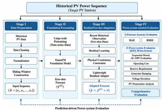
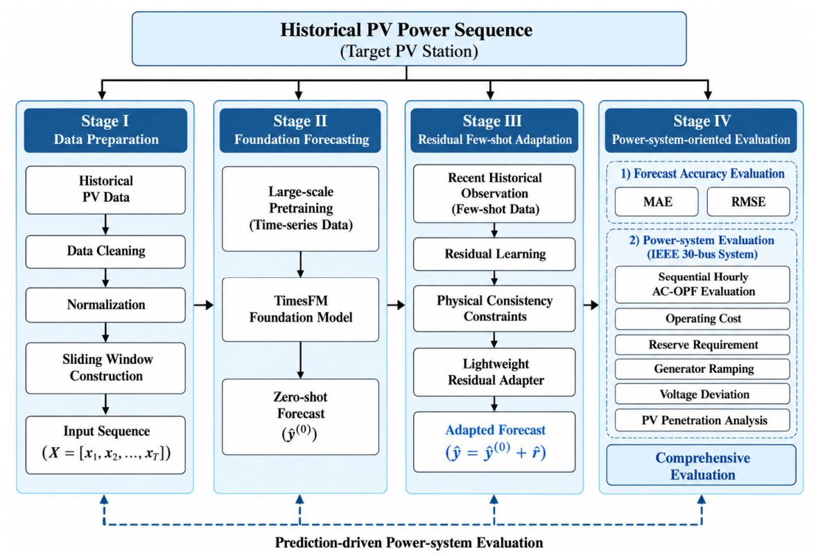
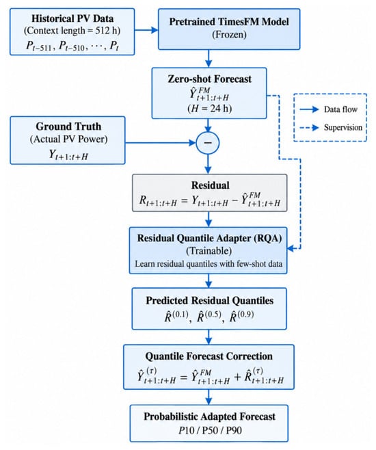
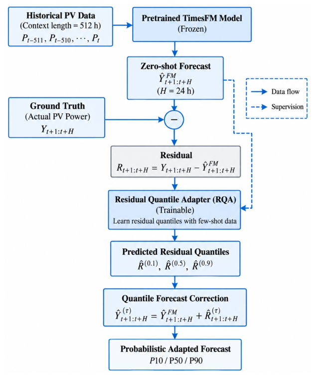
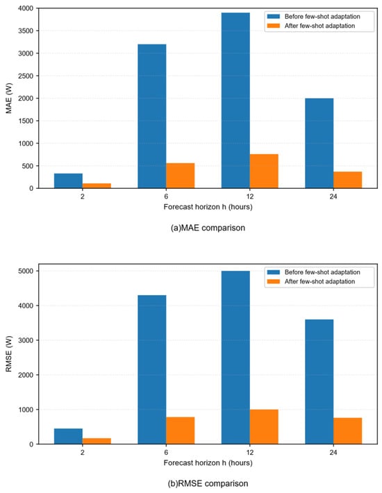
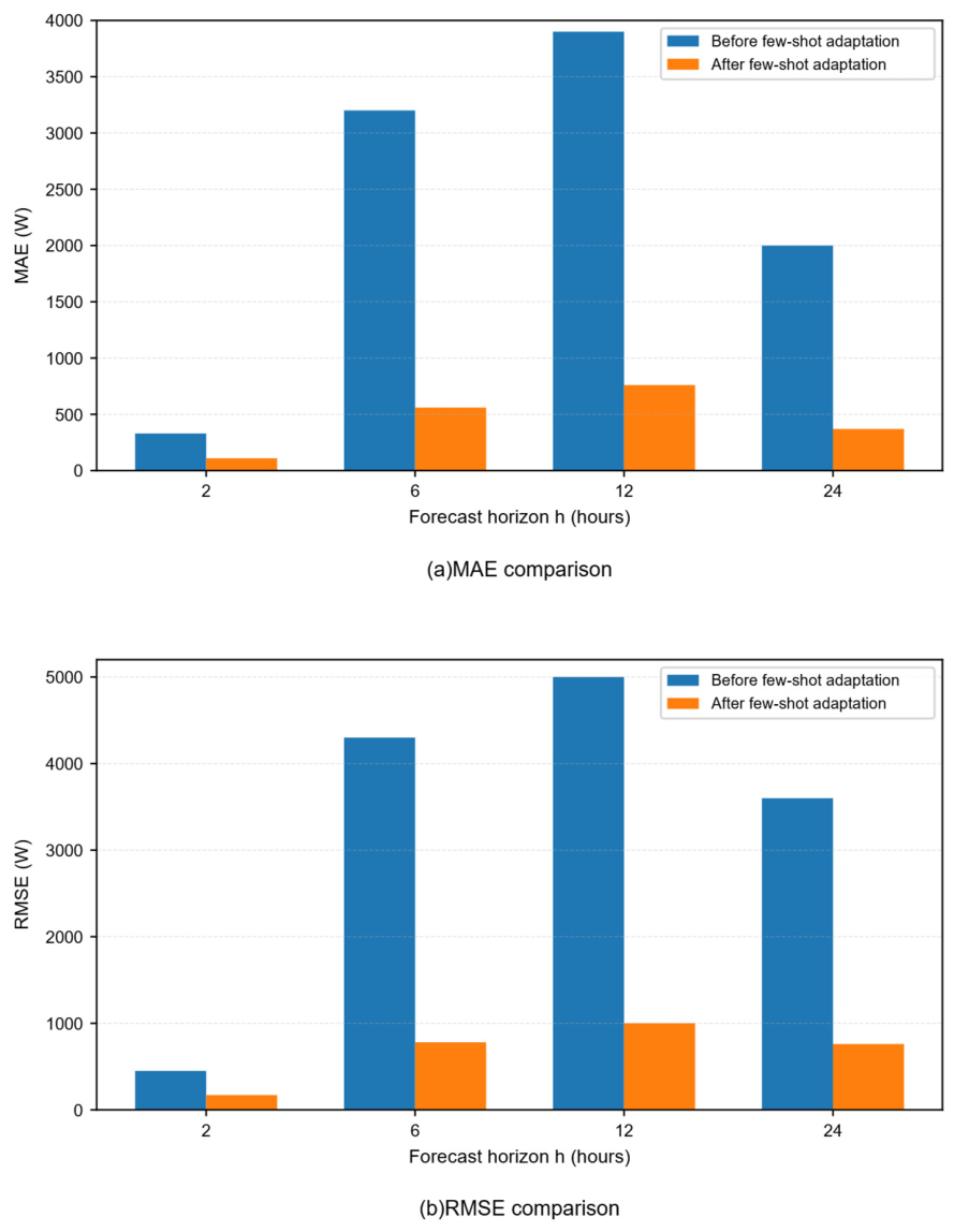
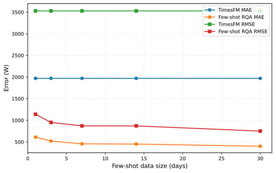
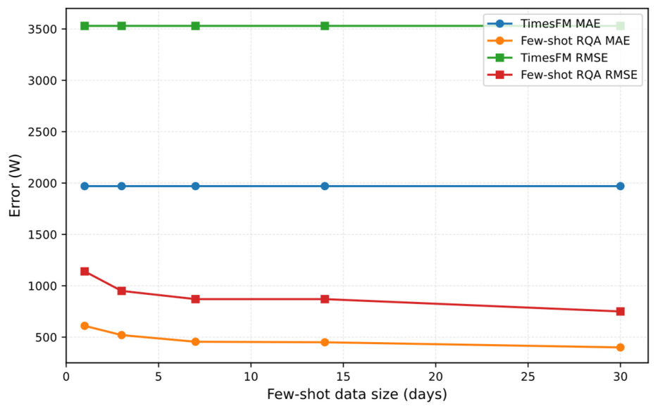
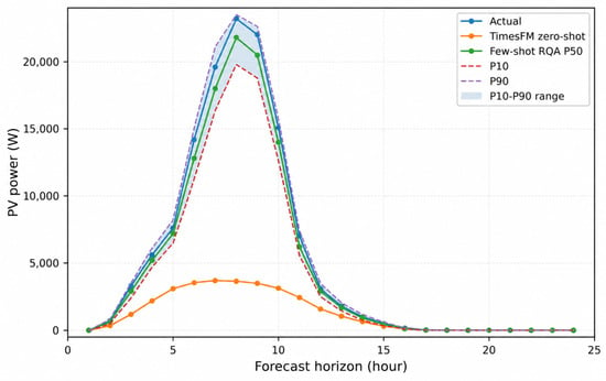
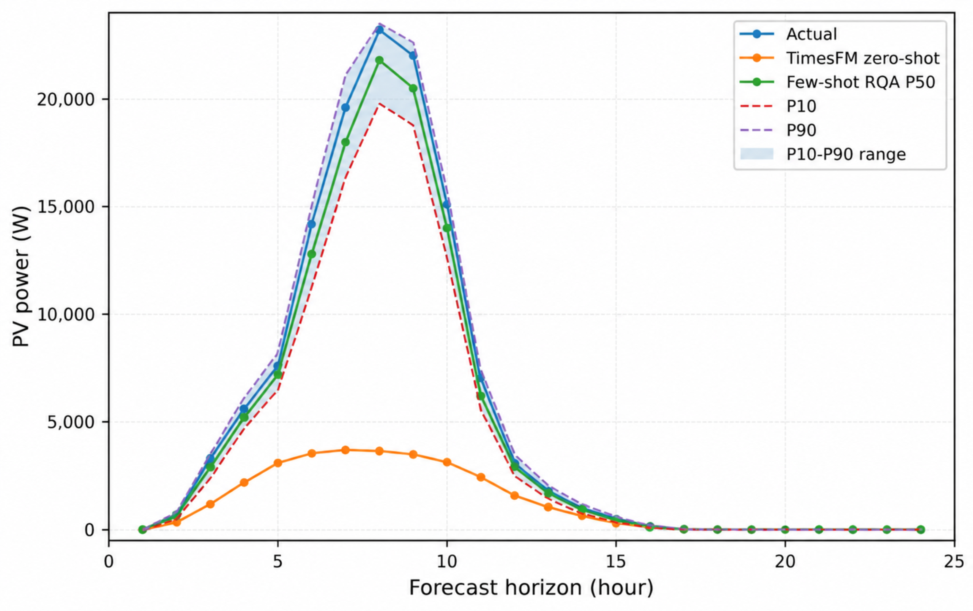
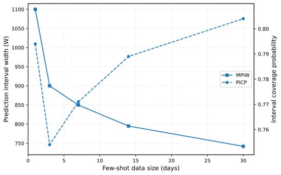
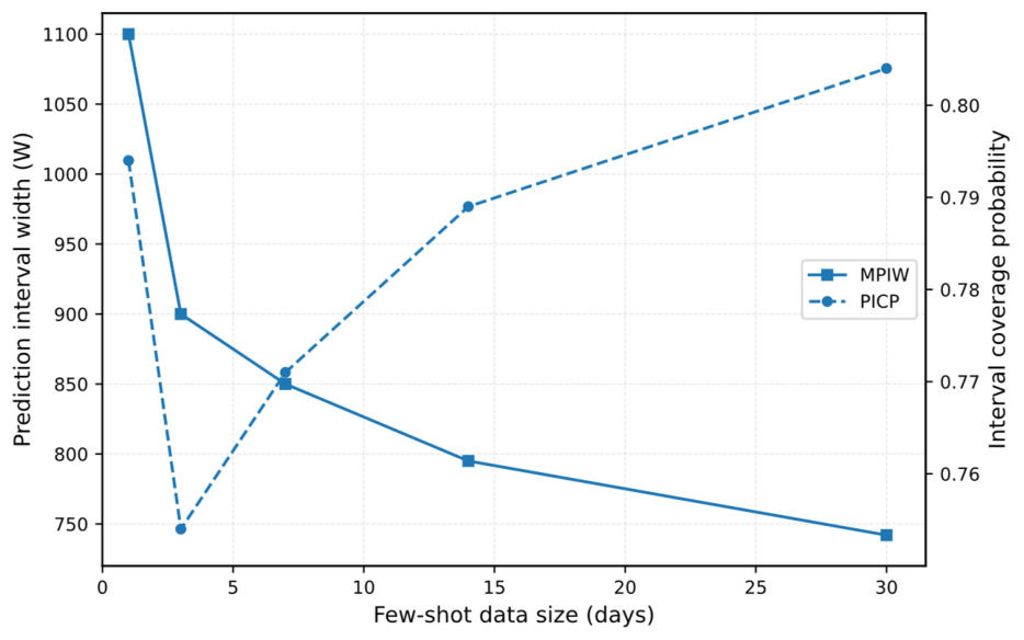
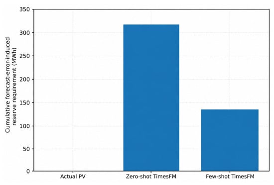
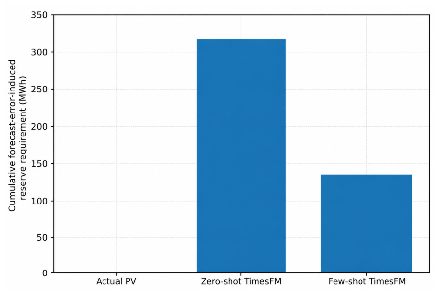
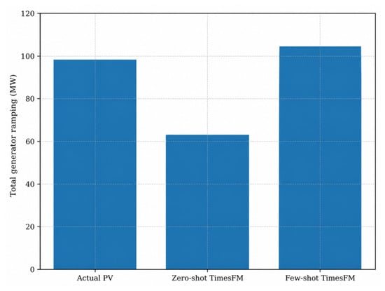
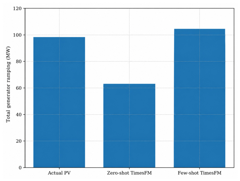
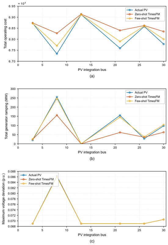
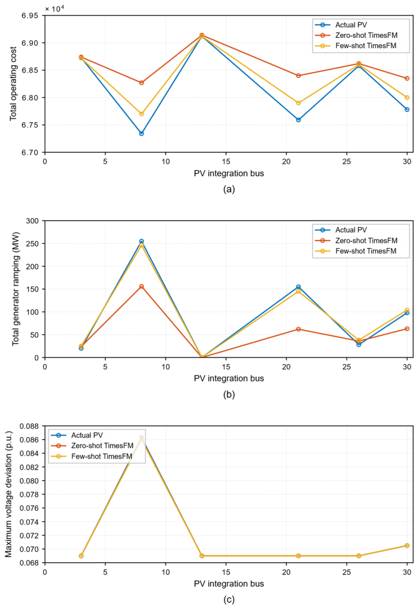
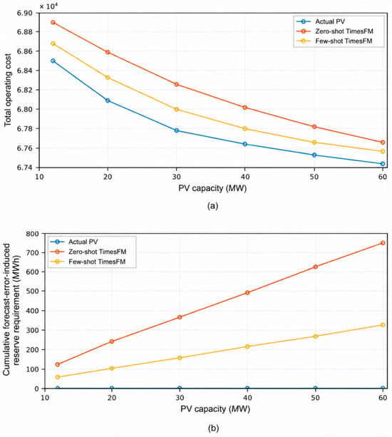
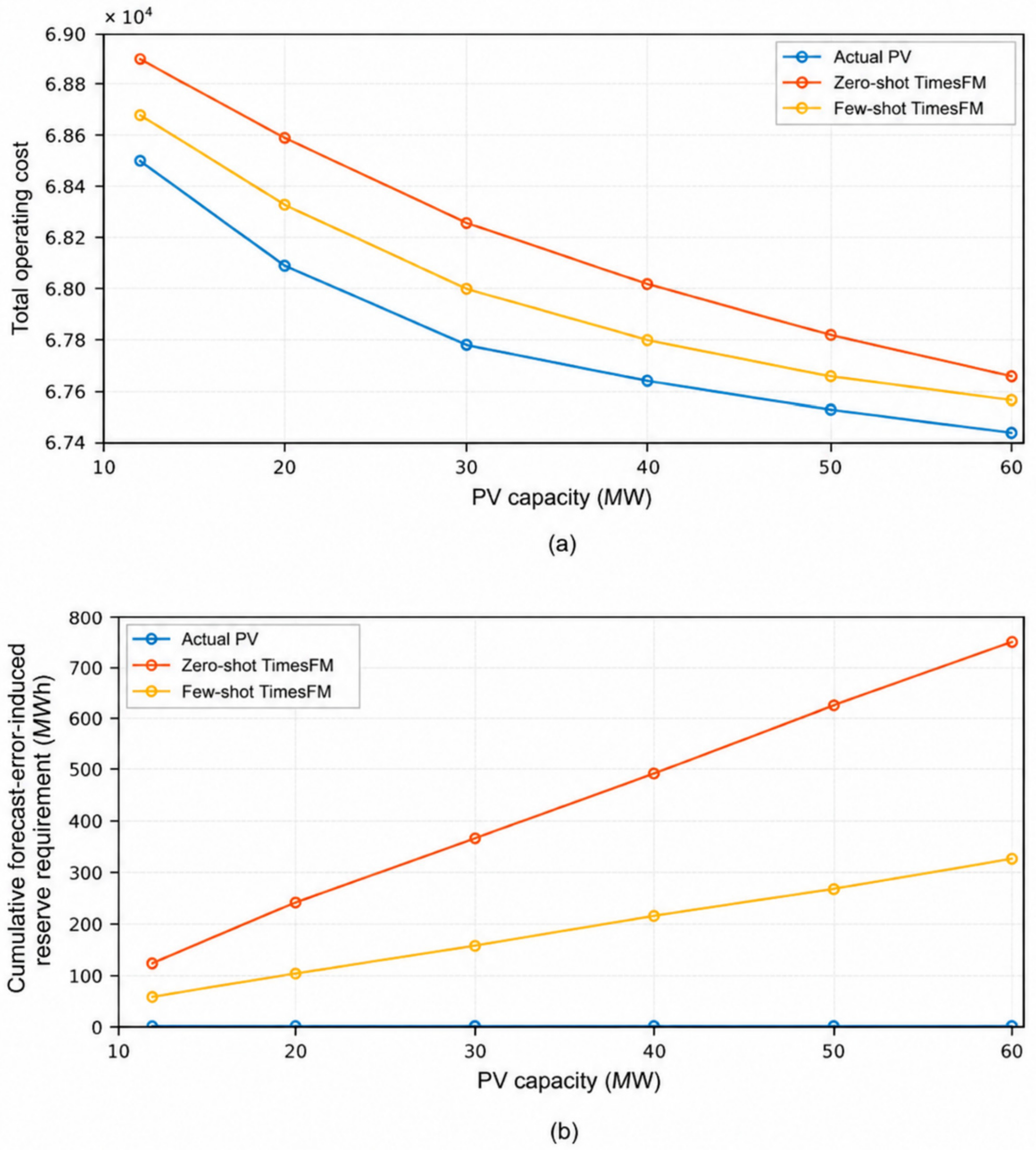

Disclaimer/Publisher’s Note: The statements, opinions and data contained in all publications are solely those of the individual author(s) and contributor(s) and not of MDPI and/or the editor(s). MDPI and/or the editor(s) disclaim responsibility for any injury to people or property resulting from any ideas, methods, instructions or products referred to in the content. |
© 2026 by the authors. Licensee MDPI, Basel, Switzerland. This article is an open access article distributed under the terms and conditions of the Creative Commons Attribution (CC BY) license.