


Abstract
The power temperature coefficient (γ) of a photovoltaic–thermal (PVT) collector is usually taken from the datasheet. Determining it outdoors is difficult because irradiance and temperature vary together. This study evaluates how reliably γ can be estimated from a few field observations. Thirty observations were collected during three campaigns in Bacău, Romania, in 2024 on a 240 Wp liquid-cooled PVT collector operated at a fixed pump setting. Power normalised to 1000 W/m2 was regressed on front-surface temperature with campaign-specific intercepts. This conventional analysis yielded γ = −0.64%/°C (95% CI: −0.82 to −0.46), compared with the declared −0.45%/°C. The result was sensitive to model specification. Irradiance and panel temperature were strongly correlated (r = 0.84), and including irradiance as a covariate, which the data supported (p = 0.043), changed γ to −0.40%/°C (−0.72 to −0.09). Eleven specifications differing in covariates, first-observation exclusions and temperature variable produced estimates from −0.33 to −1.08%/°C. In one campaign, measured power averaged 19% above the nameplate-based expectation, indicating an inconsistency in the absolute measurement scale. In an hourly PVGIS-SARAH3 calculation for 2023, each 0.1%/°C change in γ altered annual electrical yield by 0.94%. The measurements are compatible with the datasheet coefficient but constrain it only to between about ±0.3 and ±0.7%/°C, depending on the specification.
1. Introduction
Photovoltaic–thermal (PVT) collectors generate electricity and recover heat from the same aperture. A fluid circulating behind the photovoltaic layer removes part of the absorbed energy, which lowers the cell temperature and supplies heat for water heating or space conditioning [1,2,3]. The concept has been developed for buildings, domestic hot water and industrial processes [4,5,6,7,8].
How much power a module loses as it warms is described by the power temperature coefficient, γ. For crystalline silicon the coefficient is negative because the open-circuit voltage falls with temperature faster than the short-circuit current rises [9,10], and values of about −0.4 to −0.5%/°C are commonly reported [9,11]. Manufacturers determine γ under controlled conditions, in which irradiance is held constant while temperature is varied, and report it relative to standard test conditions (STC) [12,13]. Performance models then apply the datasheet value to whatever operating temperature the simulation predicts [14,15].
Outdoors, that separation is not available by design. Irradiance, module temperature, spectrum and angle of incidence change together over a day, so the temperature dependence of power has to be isolated statistically or by an explicit irradiance correction. King et al. [16] described the practical difficulties of outdoor determination, non-uniform module temperature among them. Later work showed that the outcome depends on conditions and method. Gasparin et al. [17] found that the temperature coefficients of crystalline-silicon modules vary with irradiance. Senturk [18] tested datasheet coefficients against field data under different sky conditions, and Paudyal and Imenes [19] reported module- and year-dependent coefficients from an eight-year outdoor record, with a clear influence of the correction procedure. In a climatic chamber, Hudișteanu et al. [20] measured −0.46 and −0.50%/°C for small mono- and poly-crystalline modules. A further complication is that field studies usually measure a surface temperature, whereas γ refers to the cell [14,21,22].
For liquid-cooled PVT collectors the literature has concentrated on thermal management and efficiency. Reviews cover the main cooling concepts [23,24]. Individual studies have examined nanofluids [25,26,27], modified tubes and absorber geometries [28,29,30,31], jet impingement and bifacial designs [32,33], porous media combined with phase-change materials [34], and the effect of operating parameters on energy and exergy performance [35,36,37]. System-level work has addressed PVT-assisted heat pumps [38] and the differences between indoor and outdoor results [39]. Al Tarabsheh et al. [40] showed that the temperature of cooled cells is not uniform along the flow path and that this affects electrical output, and Dölek and Arslan [41] examined the factors that govern the efficiency of a PVT system. In nearly all of these studies γ enters as a fixed datasheet parameter. Whether a field campaign on a cooled collector can confirm or revise that parameter has received little attention.
The facility used here was described by Grigore et al. [42], who compared the measured electrical and thermal output of a SunSystem PVT 240 collector with a numerical model, using data from 2023. In that work γ was a model input. The present study uses a separate dataset acquired in 2024, in which electrical power was recorded independently of any assumed temperature coefficient.
Our initial aim was to determine γ for this collector from outdoor spot measurements by the usual route: normalise power to a reference irradiance, regress it on panel temperature, and pool the campaigns. While checking that result, we found it sensitive to choices that are seldom reported. The paper therefore asks a narrower question: how well do thirty spot observations constrain γ, and which analysis choices move the estimate? We (i) report the conventional estimate with its full statistical description, (ii) test the proportionality between power and irradiance that the normalisation assumes, (iii) quantify the influence of the first observations of each campaign and of the temperature variable, and (iv) express the resulting range of γ in annual-energy terms through an hourly calculation. The collector was examined in its normal, actively cooled mode of operation, because this is the condition in which the coefficient is applied in PVT performance models and in which a field determination on such a collector would be made. The front-surface temperature serves as a proxy for cell temperature throughout. The coefficient reported is thus a field-derived quantity, denoted γfield; it should not be read as a cell-temperature coefficient at STC.
2. Materials and Methods
2.1. Experimental Facility
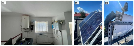
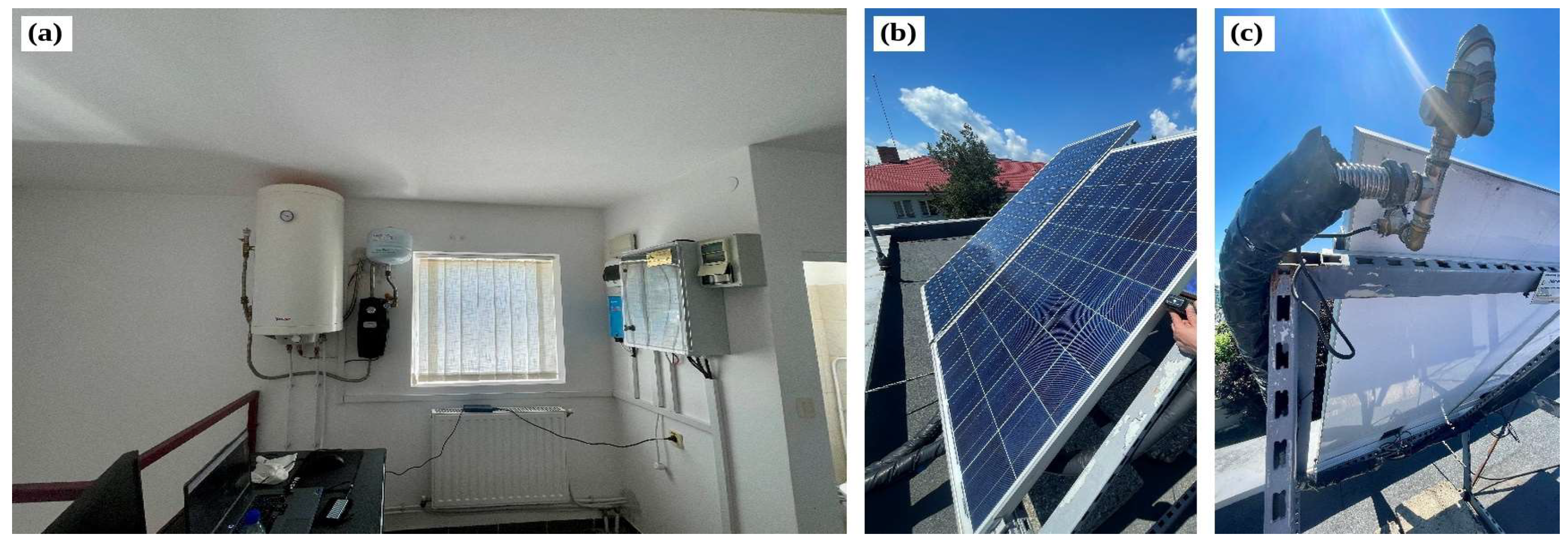
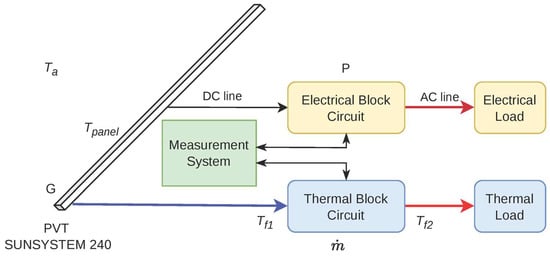
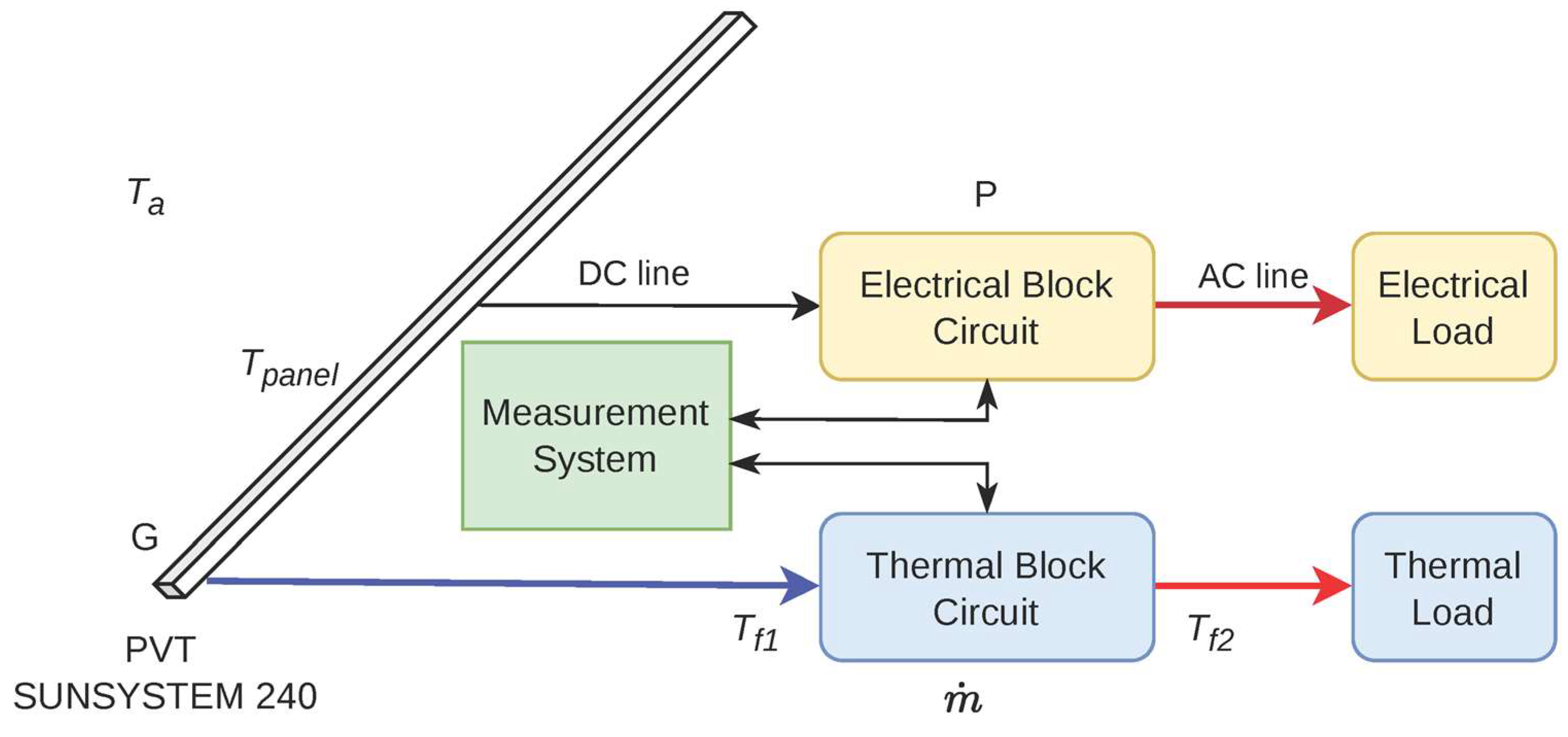
The measurements were made on the PVT test facility of the “Vasile Alecsandri” University of Bacău, Romania (46.554° N, 26.915° E) [42]. A SunSystem PVT 240 collector (NES Ltd., Shumen, Bulgaria) is mounted on the laboratory roof at a tilt of 45° and an azimuth of 0° (south). It combines a 60-cell polycrystalline module with a copper absorber through which a 50% propylene glycol–water mixture circulates. The collector has a gross area of 1.62 m2, a rated power of 240 Wp, a fluid content of 1.17 L and a declared power temperature coefficient of −0.45%/°C. The rated power corresponds to an efficiency of 0.148 on the gross area. At standard test conditions, the module has an open-circuit voltage of 37.2 V, a short-circuit current of 8.52 A, and its maximum-power point at 30.6 V and 7.84 A. The copper pipe register lies behind an aluminium plate and is insulated at the rear with 20 mm of rigid polyurethane, and the manufacturer recommends a flow rate of 1.5–2.5 L/min. The 156 × 156 mm cells lie behind 3.2 mm of tempered glass, and the module efficiency is 14.7%. On the thermal side, the manufacturer gives a zero-loss efficiency of 0.559, a heat-loss coefficient of 9.13 W/(m2·K) and a nominal thermal output of 900 W. Figure 1 shows the installation and Figure 2 the arrangement of the electrical and thermal circuits.
Figure 1.
The experimental facility: (a) storage tank, pumping unit and electrical cabinet; (b) roof-mounted PVT collector; (c) hydraulic connection at the rear of the collector.
Figure 2.
Schematic of the PVT system, showing the electrical and thermal circuits and the measured quantities. Yellow, blue and green blocks denote the electrical, thermal and measurement subsystems; red arrows indicate energy delivered to the loads, the blue arrow the heat-transfer fluid leaving the collector and black arrows the DC line and measurement signals.
The thermal circuit is a closed loop in which the glycol mixture is circulated between the collector and a 100 L storage tank (Eldom Thermo; Eldominvest Ltd., Bulgaria) by a Trollino 05S pumping unit (Barberi Rubinetterie Industriali S.r.l., Italy), under a Westech WT-C1 solar controller (Westech Solar, Garching bei München, Germany). The fluid flows through the copper register at the rear of the collector, takes up the heat conducted through the laminate and the aluminium plate, and returns to the tank. As the tank warms during the day, the collector inlet temperature rises with it (Table 1). The pump ran at its third speed setting in all campaigns, for which the nominal flow rate of the pump is 4.2 L/min. This value is higher than the 1.5–2.5 L/min recommended for the collector [42], and the actual flow depends on the pressure drop of the circuit. The flow was not measured. The nominal value is used wherever a flow rate is needed, and the consequences are discussed in Section 2.3, Section 4.1 and Section 4.4.
Table 1.
Measurement campaigns and ranges of the measured quantities. The pump operated at the same setting throughout (nominal flow rate 4.2 L/min).
On the electrical side, the module feeds a Victron SmartSolar MPPT 100/20 (Victron Energy B.V., Almere, The Netherlands) charge controller within a battery-based system that includes a Victron Energy AGM 12 V, 60 Ah battery (Victron Energy B.V., Almere, The Netherlands), a MultiPlus 500 VA inverter/charger (Victron Energy B.V., Almere, The Netherlands), and a Cerbo GX monitoring device (Victron Energy B.V., Almere, The Netherlands). The electrical power P used in this study is the PV power reported by the charge controller and logged through the Victron Remote Management (VRM) portal. Contemporaneous VRM records from the three experimental campaigns indicate that the battery remained at or close to 100% state of charge during much of the measurement periods. However, the charger operating stage (bulk, absorption, or float) at the individual observation times was not included in the experimental dataset and is no longer available retrospectively. Consequently, unrestricted maximum-power-point operation cannot be independently verified for every observation.
2.2. Instruments and Measurement Campaigns
In-plane global irradiance G was measured directly in the plane of the PVT collector using a Multimetrix SPM72 solar power meter (Chauvin Arnoux, France). These measurements provided the irradiance values used in all subsequent calculations and regression analyses. A second solar power meter (Amprobe SOLAR-100, Amprobe, Everett, WA, USA), positioned in the same plane, was used intermittently during the experiments to check the consistency of the irradiance readings. These comparison readings were not systematically recorded and were therefore not used in the quantitative analysis. The panel front-surface temperature (Tpanel) was measured using a Testo 865s infrared thermal-imaging camera (Testo SE & Co. KGaA, Titisee-Neustadt, Germany), with the emissivity set to 0.95 for the glass surface. The instrument was supplied with a manufacturer-issued calibration and conformity protocol documenting verification against a reference blackbody at 0 and 80 °C, with deviations within the specified tolerance of ±2 °C. For each observation, the camera was successively directed towards five locations on the panel surface (the four corners and the centre), and the arithmetic mean of the five temperature readings was used as Tpanel. The camera was hand-held at a distance of about 0.3 m from the collector, approximately normal to the glass. Glass is opaque in the long-wave infrared band used by the camera, so the reading refers to the outer surface of the front glass and not to the cells. Because the coefficient is derived from the slope of power against temperature, a constant offset in the temperature reading leaves the slope unchanged and enters only through the reference power, whereas a proportional (gain) error changes the slope directly. Both cases are quantified in Section 3.6. Fluid temperatures at the collector inlet Tf1 and outlet Tf2 were measured using PT1000 sensors (±0.3 °C) placed in the inlet and outlet pipes at the collector connections, and ambient temperature Ta using a Testo 410-2 instrument (±0.5 °C). Wind speed and relative humidity were read only occasionally and were not recorded systematically, so they are not part of the dataset.
Three campaigns were carried out on 26 March, 30 April and 21 May 2024. In each, ten observations were taken at 30 min intervals, from 09:00 to 13:30 local time in March and May and from 11:00 to 15:30 in April. Readings were taken when the irradiance display showed no marked short-term fluctuation; no automated stability criterion was applied. Table 1 summarises the conditions. The individual observations are listed in Tables S1–S3.
2.3. Thermal Quantities
The heat removed by the fluid was estimated as
with cp = 3581.4 J/(kg·K) and ρ = 1036.1 kg/m3 for the 50% mixture at the mean fluid temperature [43], which gives = 0.0725 kg/s at the nominal flow rate. The nominal flow rate was used only for the thermal calculations and was not an input to the regression models used to estimate the electrical temperature coefficient. Although the pump operated at a fixed speed setting, the actual flow rate was not monitored and cannot be assumed to have remained strictly constant. The tolerances of the two sensors combine to ±0.42 K on the temperature difference, or ±110 W on Q, before any allowance for the unmeasured flow rate. Q is proportional to the flow rate. If the actual flow were within the range recommended by the manufacturer, 1.5–2.5 L/min, Q and the thermal efficiency would be lower than the values reported here by a factor of 0.36–0.60. Because the observed differences were between 0.5 and 1.9 K, Q and the thermal efficiency ηth = Q/(G A) are reported only as indications of the operating regime. The same applies to the overall efficiency ηtot = ηth + ηel, where ηel = P/(G A) is the electrical efficiency. All three are given per campaign as the mean and standard deviation of the ten observations (Table 2).
Table 2.
Campaign-mean efficiencies of the collector (mean ± standard deviation of the ten observations). ηth and ηtot are based on the nominal flow rate of 4.2 L/min. The last two columns give the uncertainty of an individual ηth value due to the fluid-temperature sensors and the range of the campaign mean of ηth for a flow rate of 1.5–2.5 L/min. The ± values are standard deviations of the ten observations; they describe the variability within each campaign and are not measurement uncertainties. No systematic uncertainty is given for ηel, although nameplate ratios of up to 1.26 (Section 3.1) show that the absolute scale of the electrical data may be biased by up to about a quarter.
2.4. Irradiance Normalisation and the Conventional Model
The simplest description of module power treats the effects of irradiance and temperature as separable [9,15]:
where Pref is the power at reference conditions, G0 = 1000 W/m2 and Tref = 25 °C. Dividing by irradiance gives the normalised power:
which, under Equation (2), depends on temperature alone. Pnorm is a regression variable obtained by scaling. It is not a measurement at 1000 W/m2, and the scaling stops short of the I–V curve translation to STC specified in IEC 60891 [12].
In the conventional analysis (specification A), is modelled as a linear function of with a separate intercept for each campaign j and a common slope b:
The campaign intercepts absorb differences between measurement days that are unrelated to temperature, such as soiling, spectrum or a shift in the irradiance scale. The assumption of a common slope was tested by adding campaign-by-temperature interaction terms and comparing the nested models with an F test (analysis of covariance, ANCOVA).
2.5. Relaxing the Proportionality Assumption
Equation (3) removes the effect of irradiance only if power is proportional to G at a given temperature. To test this, G was added to the model as a covariate (specification B):
Under exact proportionality c = 0. A non-zero c means that normalised power still varies with irradiance at a fixed panel temperature, for physical or instrumental reasons. Because the irradiance on a fixed plane rises and falls with the time of day, a variant with the clock time t (in hours) in place of G was also fitted (specification C).
The field-derived coefficient follows from the slope and the fitted power at reference conditions:
where ā is the mean of the three campaign intercepts. The last term applies to specification B only; in specification C it is replaced by the time coefficient multiplied by a reference time of 12:00. Confidence intervals for were obtained by first-order propagation of the parameter covariance matrix through Equation (6) [44], with Student’s t at the residual degrees of freedom. The intervals therefore include the uncertainty of both b and and their correlation.
2.6. First-Observation Influence Diagnostics and Temperature Variable
Leverage and Cook’s distance [45] were computed for each campaign regression and for the pooled model. To assess sensitivity to the earliest observations in each campaign, two alternative datasets were examined: one omitting the first observation of each campaign and one omitting the first two. A further sensitivity analysis retained only observations for which Tpanel > Tf1. These exclusions were used solely to assess sensitivity to observation selection and were not interpreted as evidence of a specific transient operating state.
The mean fluid temperature, Tfm = (Tf1 + Tf2)/2, was tried as an alternative temperature variable (specification D) to assess how the estimated coefficient depends on the choice of temperature proxy in a liquid-cooled collector. The mean fluid temperature does not represent the cell temperature and was used only for sensitivity analysis.
Eleven specifications result (Section 3.5). Specification A0, the conventional analysis on all observations, was the analysis originally planned. The other ten are sensitivity analyses, and none was chosen in advance as the preferred one. Residual normality (Shapiro–Wilk) and homoscedasticity (Breusch–Pagan) were checked for A0 and B0. All models were fitted by ordinary least squares in Python 3.13.9 (statsmodels) and reproduced with spreadsheet functions in Microsoft Excel 2016 in the workbook supplied with the data.
Three further checks concern the temperature measurement and the ambient conditions. First, models A0 and B0 were refitted under two hypothetical temperature-error scenarios: a constant offset of ±2 °C, chosen to match the camera’s specified tolerance, and a proportional (gain) error of ±2%. These scenarios were used to assess the sensitivity of the regression estimates and do not constitute a complete propagation of measurement uncertainty. Second, to examine the difference between the front glass and the cells, the cell temperature was represented as Tpanel + kG and the models were refitted with this quantity, for k = 3 and 6 K per 1000 W/m2. These values were selected as illustrative sensitivity scenarios, informed by temperature differences reported for conventional PV modules [14], rather than as measured or validated bounds for the glass-to-cell temperature difference in the liquid-cooled PVT collector. Third, the ambient temperature Ta was added as a covariate to A0 and B0. Wind speed and humidity were not available for a similar test.
2.7. Comparison with the Nameplate Rating
As a check on the absolute scale of the measurements, each measured power was compared with the value expected from the rating and the declared coefficient = −0.45%/°C:
with = 240 W.
2.8. Annual-Energy Calculation
To express differences in γ in energy terms, hourly in-plane irradiance and air temperature for 2023 were taken from the PVGIS-SARAH3 database [46,47] for the site and for the plane of the collector. The panel temperature in each hour was estimated from a linear relation fitted to the 30 observations,
with and in °C and G in W/m2 (R2 = 0.80; residual standard error 4.4 °C). The relation has the same linear form as common correlations for module temperature [11,48]. Hourly power was calculated from Equation (2) with = 240 W and summed over the 8760 h of the year to give the annual energy E(γ). The relative difference with respect to the declared coefficient is
so that positive values indicate a lower yield than the datasheet coefficient would predict. Equation (2) is linear in γ, which makes ΔE proportional to γ − ; one sensitivity figure, in per cent of annual yield per 0.1%/°C, therefore describes the whole calculation.
The calculation measures sensitivity; it does not predict the yield of the system. Equation (8) contains no fluid temperature, although the inlet-fluid temperature may influence the operating temperature of a liquid-cooled PVT collector. Its independent contribution could not be established from the present measurements, and the hourly series extends beyond the measured ranges of irradiance and temperature.
3. Results
3.1. Operating Conditions and Absolute Scale
Across the 30 observations, irradiance ranged from 314 to 890 W/m2 and panel temperature from 13.5 to 46.2 °C (Table 1). The fluid gained heat in every observation. The temperature rise was between 0.5 and 1.9 K, which corresponds to Q between 130 and 494 W at the nominal flow rate. Table 2 gives the campaign-mean efficiencies. The electrical efficiency decreased from 0.172 in March to 0.134 in May, while the thermal efficiency increased from 0.28 to 0.34, so that the overall efficiency stayed between 0.45 and 0.48. The decrease in ηel follows mainly the change in the nameplate ratio discussed below and does not indicate a change in collector performance. The sensor tolerances alone correspond to about ±0.10 to ±0.12 on each individual value of ηth, and the unmeasured flow rate adds a one-sided uncertainty: with a flow of 1.5–2.5 L/min the campaign means of ηth would fall to 0.10–0.20. These figures establish that the collector was being cooled and that the three campaigns operated in a similar thermal regime. They do not support a finer thermal analysis.
The electrical data show a discrepancy in absolute scale. The ratio r of Equation (7) averaged 1.19 on 26 March (range 1.10–1.26), 1.10 on 30 April (1.02–1.19) and 0.97 on 21 May (0.86–1.06). Put differently, the apparent electrical efficiency P/(GA) reached 0.192 in March, against the 0.148 implied by the rated power. A module does not exceed its rating by a fifth at these temperatures. The March and April data therefore indicate a systematic inconsistency in the absolute measurement scale. Its source cannot be identified retrospectively from the available data; possible contributions include the irradiance measurement and the power reported by the charge controller. Because the ratio changes from day to day (1.19, 1.10 and 0.97), a constant calibration error of the irradiance meter cannot explain it alone; day-dependent effects such as the angle of incidence, the solar spectrum, soiling of the glass or the charging stage of the controller are more likely contributors. Because the bias differs between campaigns, campaign-specific intercepts are indispensable, and the absolute level of has no physical meaning. Only the variation within campaigns is used below.
The first observations of each campaign also differed from the subsequent measurements. On 30 April, the first reading gave Tpanel = 14.8 °C, while the inlet-fluid temperature was 28.4 °C and the ambient temperature was 14.4 °C. On 21 May, the first reading (17.2 °C) was likewise below the inlet-fluid temperature (21.2 °C), and two later observations showed smaller inversions of less than 1 K. On 26 March, the inlet-fluid temperature increased from 12.5 to 24.3 °C between 09:30 and 10:00. These observations identify the earliest measurements as potentially influential points and also illustrate a limitation of using front-glass temperature as a proxy for cell temperature. Their influence on the estimated temperature coefficient is examined explicitly in Section 3.3.
3.2. Conventional Analysis
Regressed separately, the three campaigns gave slopes of −1.91, −1.61 and −1.62 W/°C, all significant at the 1% level, and coefficients of −0.660, −0.595 and −0.675%/°C (Table 3). The interaction test gave no evidence of different slopes (F(2, 24) = 0.14, p = 0.87). With ten observations per campaign, this test has little power, so the absence of evidence for different slopes does not establish that the slopes are equal. The intercepts, in contrast, differed strongly (F(2, 26) = 34.3, p < 0.001), in line with the scale differences noted in Section 3.1.
Table 3.
Separate regressions of normalised power on panel surface temperature for each campaign (n = 10), with the correlation between irradiance and panel temperature and the influence statistics of the first observation of the day. SE: standard error.
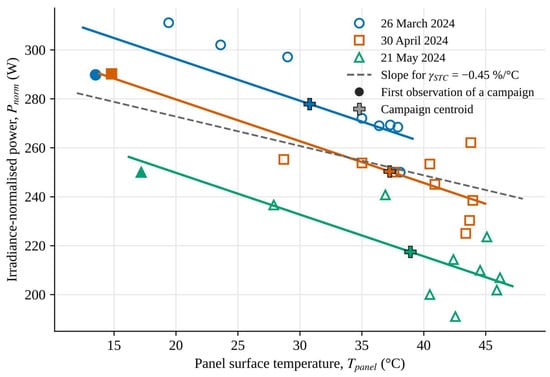
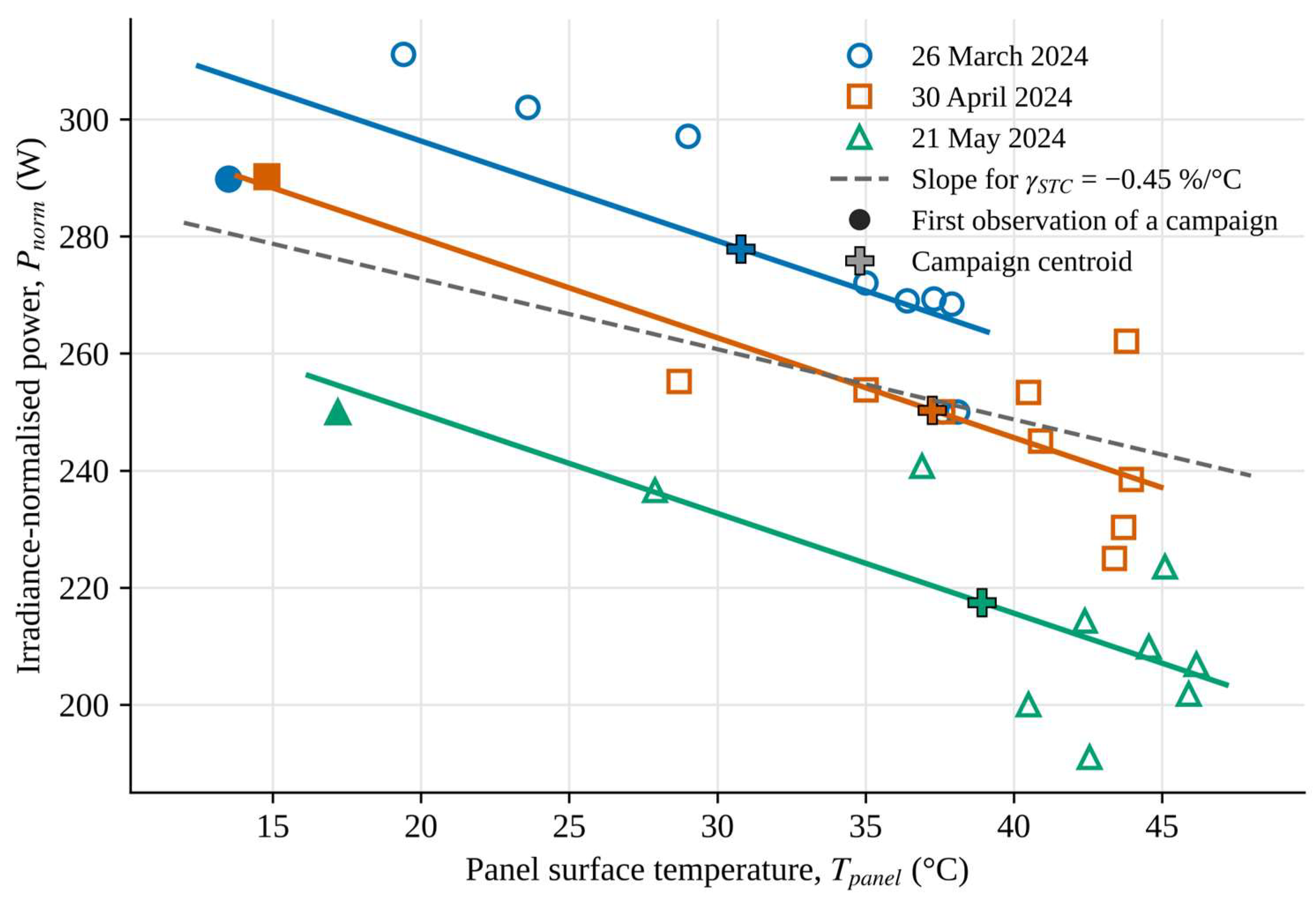
The common-slope model has b = −1.71 W/°C (standard error 0.25 W/°C), R2 = 0.87 and a residual standard error of 12.0 W. With = 266.7 W, Equation (6) gives = −0.64%/°C with a 95% confidence interval of −0.82 to −0.46%/°C (Figure 3). The declared value of −0.45%/°C lies just outside this interval (p = 0.040). The residuals showed no departure from normality (Shapiro–Wilk p = 0.17) or from constant variance (Breusch–Pagan p = 0.91).
Figure 3.
Irradiance-normalised power against panel surface temperature, with the common-slope fit of specification A0 (solid lines, in the colour of each campaign). Filled symbols mark the first observation of each campaign. Crosses mark the campaign centroids, through which the fitted lines pass. The dashed line shows the slope that corresponds to the declared coefficient, drawn through the pooled reference power.
In Figure 3 the vertical position of each line is set by the campaign intercept aj, and with a common slope, each line passes through the centroid of its campaign. The March line lies highest because the March data carry the largest scale excess (mean r = 1.19, Section 3.1). The vertical spacing of the lines therefore reflects the differences in absolute scale between the days and has no thermal meaning. Within March, the points are not scattered at random about the line. The residuals are −17.6 W for the first observation, between +11.9 and +16.2 W for the next three and −15.4 and −16.3 W for the last two, so the data lie below the line at both ends of the morning. A single linear slope cannot follow this pattern, which is examined in Section 3.4.
Read on its own, this result would mean a temperature coefficient about 40% larger in magnitude than the datasheet value, consistent over three days. Section 3.3 and Section 3.4 examine whether this reading holds.
3.3. Influence of the First Observations
In the single-campaign fits the first observation dominates. Its leverage is 0.51, 0.75 and 0.69 for March, April and May, against a mean leverage of 0.20, and Cook’s distance reaches 2.73 for the first March point (Table 3). Each of these points lies 6 to 14 °C below the next one on the temperature axis (Figure 3), and in April and May eight of the ten observations fall within a band of about 9 °C. Without its first point, the April regression is no longer significant (b = −1.16 W/°C, p = 0.19).
Pooling moderates this dependence, since the common slope draws on all three campaigns. In the pooled model, the largest leverage is 0.32 and the largest Cook’s distance is 0.21 (Table S4), and omitting any single observation moves γfield only between −0.70 and −0.61%/°C. Removing the first observations as a group has a larger effect and steepens the slope: γfield becomes −0.79%/°C without the first observation of each campaign (A1) and −0.97%/°C without the first two (A2). Restricting the data to observations with Tpanel > Tf1 (A3) gives −0.67%/°C. Thus, inclusion of the first observations shifts the conventional estimate towards zero. The comparatively large magnitudes obtained under A1 and A2 indicate that the estimated coefficient is sensitive to observation selection and should not be interpreted as a temperature effect alone.
3.4. Residual Dependence on Irradiance
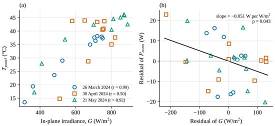
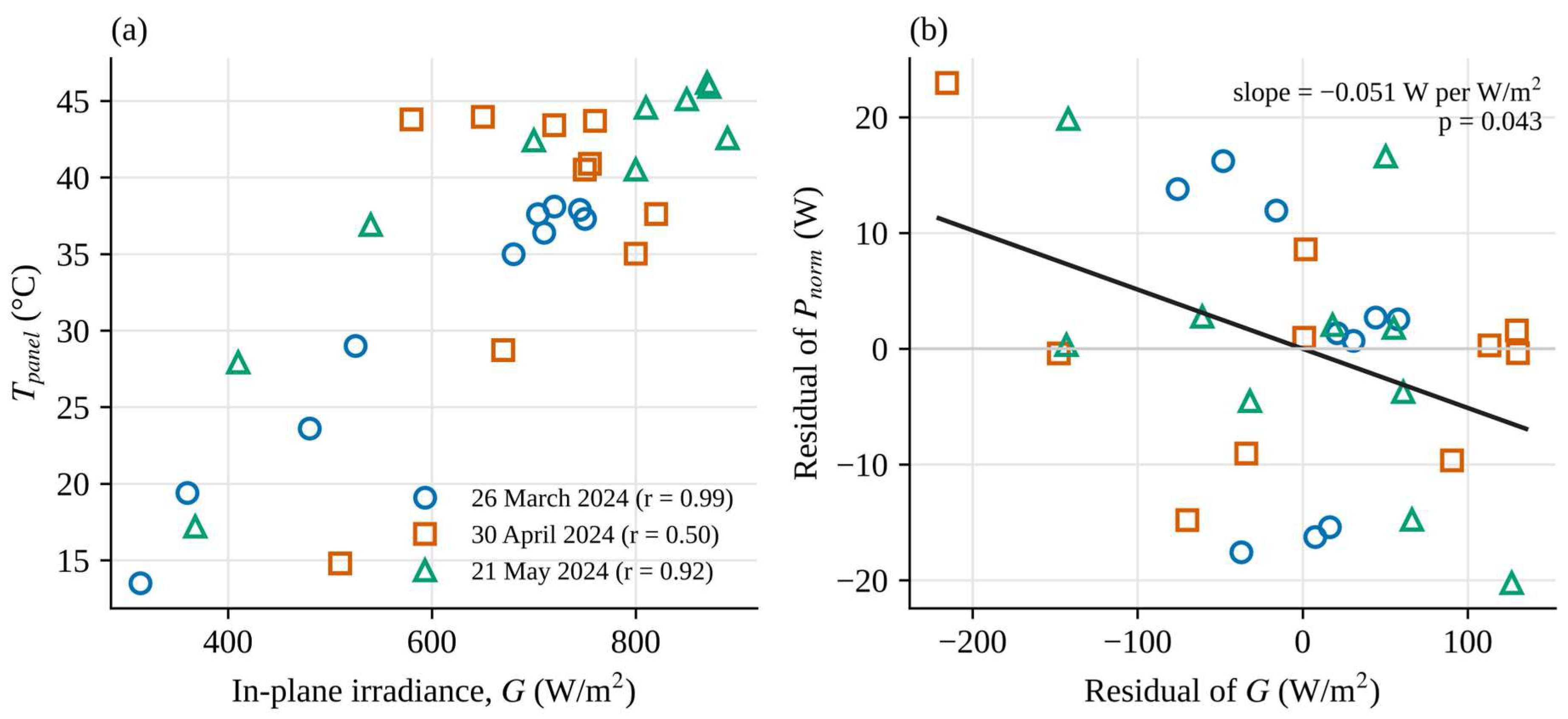
Panel temperature and irradiance were closely correlated: r = 0.84 over all observations, and 0.99, 0.50 and 0.92 within the March, April and May campaigns (Figure 4a). In March the two variables are almost interchangeable.
Figure 4.
(a) Panel surface temperature against in-plane irradiance, with the correlation coefficient of each campaign. (b) Added-variable plot for irradiance in specification B0: residuals of normalised power and of irradiance after each has been regressed on the campaign indicators and on panel temperature. Both axes show deviations from fitted values, centred on zero, and not power or irradiance themselves; negative values therefore do not indicate negative power. The slope of the line equals the coefficient c of Equation (5).
The difference between the campaigns follows from the timing of the measurements. The March series covered the morning of a clear day (09:00–13:30). Irradiance rose from 314 to 750 W/m2, the inlet-fluid and ambient temperatures rose with it, and panel temperature followed irradiance almost exactly. The April series (11:00–15:30) was centred on solar noon. Irradiance varied only between 510 and 820 W/m2, while the ambient temperature rose from 14.4 to 25.6 °C and the inlet-fluid temperature from 28.4 to 36.0 °C, so panel temperature stayed above 43 °C through the afternoon as irradiance decreased. The May series was again a morning series. Its correlation is lower than in March mainly because panel temperature fell from 45.9 to 40.5 °C during the last hour while irradiance remained between 800 and 890 W/m2; the recorded variables do not identify the cause. The low correlation in April depends largely on its first observation, which combines a panel temperature of 14.8 °C with an inlet-fluid temperature of 28.4 °C at 510 W/m2 and is physically doubtful (Section 3.1). Without it, panel temperature and irradiance are practically uncorrelated (r = −0.22), and the April slope becomes −1.16 W/°C, or about −0.44%/°C, close to the datasheet value and to specification B0. With p = 0.19, however, this estimate is not statistically significant. The April data therefore show the value of decoupling temperature from irradiance (Section 4.3) rather than providing a precise estimate.
When G is added to the model (B0), its coefficient is c = −0.051 W per W/m2 (standard error 0.024, p = 0.043). At a given panel temperature, normalised power is about 5 W lower for every additional 100 W/m2 (Figure 4b). In Figure 4b each point is the residual of Pnorm plotted against the residual of G, both obtained after the campaign and panel-temperature effects have been removed, which is why the values scatter around zero. The temperature slope falls to b = −0.97 W/°C (standard error 0.42 W/°C, p = 0.028), and with = 242.1 W at the coefficient becomes = −0.40%/°C (95% CI −0.72 to −0.09). The fit improves modestly: the adjusted R2 rises from 0.854 to 0.871, and the Akaike information criterion falls from 238.1 to 235.1. The variance inflation factor of the temperature term is 3.6, the test for equal slopes remains non-significant (F(2, 23) = 1.31, p = 0.29), and the residual checks are again passed (Shapiro–Wilk p = 0.30; Breusch–Pagan p = 0.77).
The time-of-day variant behaves similarly. Normalised power decreased by 6.0 W per hour at a fixed panel temperature (p = 0.024), and = −0.35%/°C (−0.66 to −0.03) (C0). Irradiance and clock time are themselves correlated in these campaigns, and the data cannot say which of the two describes the residual trend better.
A regression of the raw power on G and , without normalisation or campaign terms, gives P = 52.2 + 0.213 G − 0.90 (W). The temperature term is not distinguishable from zero (p = 0.14), and the constant of 52 W is incompatible with strict proportionality between power and irradiance.
3.5. Summary of the Specifications
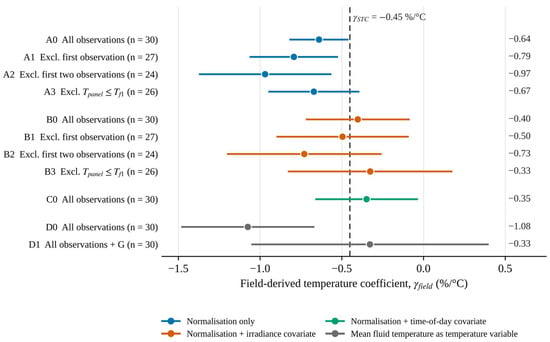
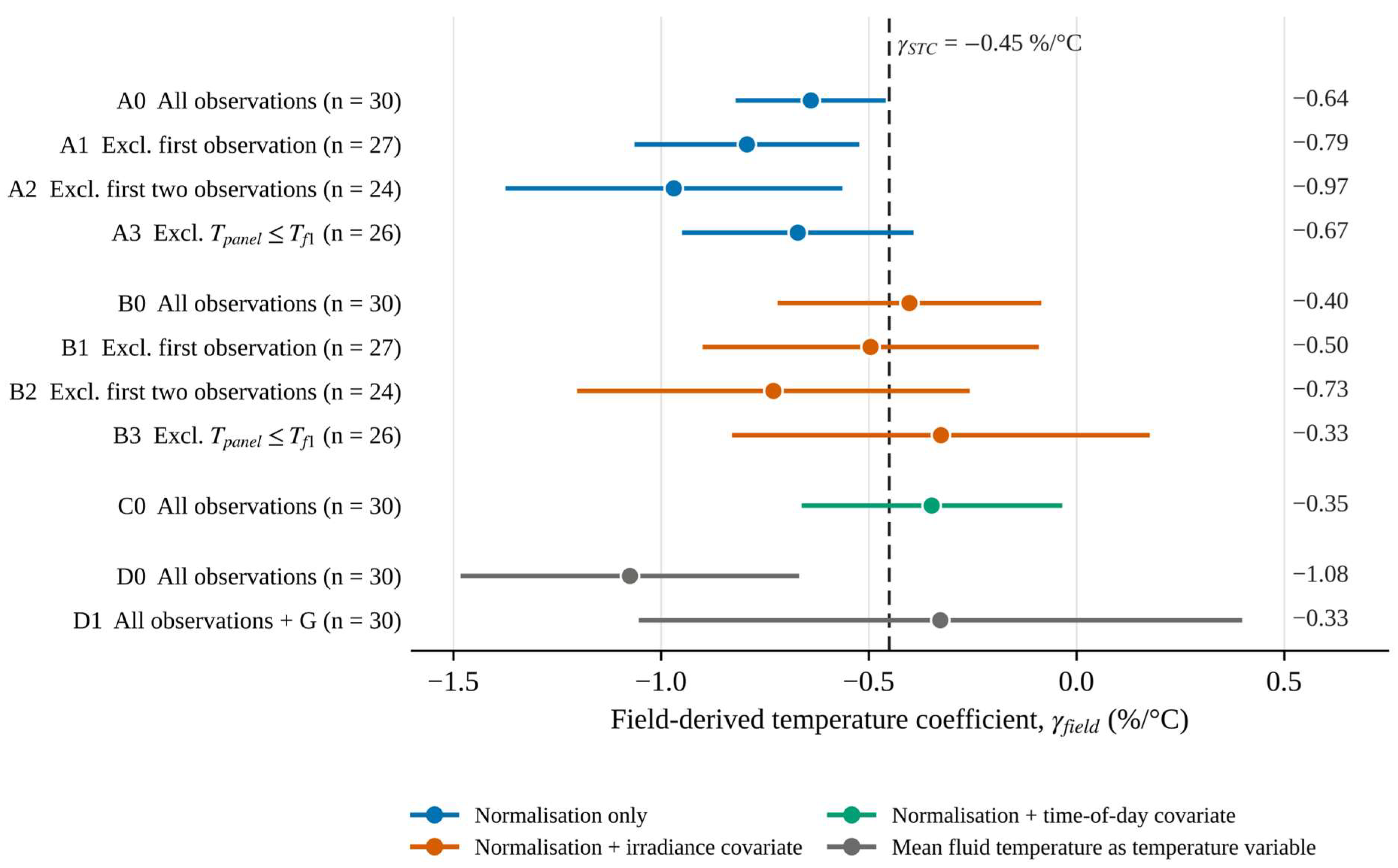
Table 4 and Figure 5 collect the eleven specifications. The point estimates run from −0.33 to −1.08%/°C and fall into two groups. The four specifications that rely on normalisation alone (A0–A3) give −0.64 to −0.97%/°C, and three of their four intervals exclude the declared value. The five that allow a residual dependence on irradiance or time (B0–B3 and C0) give −0.33 to −0.73%/°C, and every interval includes −0.45%/°C. With the mean fluid temperature as the temperature variable, the contrast is sharper still: −1.08%/°C without the irradiance covariate (D0) and −0.33%/°C with it (D1), the latter with an interval from −1.05 to +0.40%/°C.
Table 4.
Field-derived temperature coefficient under the eleven specifications. All models include campaign-specific intercepts. t: time of day; Tfm: mean fluid temperature; SE: standard error; CI: confidence interval. The last column tests the hypothesis that γfield equals the declared coefficient.
Figure 5.
Field-derived temperature coefficient and 95% confidence interval for the eleven specifications of Table 4. The dashed line marks the declared coefficient.
The half-width of the 95% interval is 0.18%/°C for A0 and between 0.31 and 0.50%/°C for the specifications of groups B and C. The conventional analysis has the narrowest interval because it makes the strongest assumption.
3.6. Sensitivity to the Temperature Measurement and Ambient Conditions
Under the hypothetical temperature-error scenarios defined in Section 2.6, the estimated coefficient showed limited sensitivity to constant offsets and proportional errors. A constant temperature offset does not change the fitted slope, so the offset scenario is reassuring only by construction. The proportional-error scenario provides a complementary assessment of the sensitivity of the estimated coefficient to a hypothetical change in the temperature scale.
The assumed emissivity of 0.95 introduces an additional source of uncertainty in the infrared temperature measurements. If the actual emissivity differed from this value, the resulting temperature error would depend on the surface temperature and the reflected apparent temperature, which was not independently measured. Consequently, the magnitude and temperature dependence of this error cannot be established from the available data. The hypothetical offset and gain scenarios examined above indicate the sensitivity of the fitted coefficients to selected temperature perturbations, but they do not quantify the uncertainty associated with emissivity or exclude other systematic temperature-dependent errors. Errors related to reflected radiation and viewing geometry were also not independently quantified.
Hansen and Farr [49] attributed systematic differences between outdoor and indoor temperature coefficients to bias in measured module temperature. For a slope-based estimate, such bias is particularly relevant when it varies with operating conditions, as may occur with the difference between glass and cell temperatures.
When the cell temperature was represented as Tpanel + kG, the estimate of A0 became −0.61%/°C for k = 3 K and −0.59%/°C for k = 6 K per 1000 W/m2, while the corresponding B0 estimates were −0.40 and −0.39%/°C. Within these illustrative scenarios, the conventional estimate moved towards the datasheet value, whereas the covariate-adjusted estimate changed only slightly. However, the actual glass-to-cell temperature difference was not measured, and the assumed gradients do not represent experimentally established or conservative bounds. Using b ≈ −1.7 W/°C, a gradient of 3 K per 1000 W/m2 would correspond to an irradiance-related contribution of approximately −0.005 W per W/m2, about one tenth of the fitted coefficient c. A substantially larger gradient would therefore be required to reproduce the entire fitted irradiance term through this mechanism alone. This calculation is illustrative and does not establish the actual contribution of glass-to-cell temperature differences to the irradiance dependence.
Ambient temperature was strongly correlated with panel temperature within each campaign (r = 0.99, 0.97 and 0.87 for March, April and May), because both rose through the measurement window. When Ta was added to A0, its coefficient was −2.3 W/°C (standard error 1.8 W/°C, p = 0.21), the AIC remained practically unchanged (238.2 versus 238.1), and γfield became −0.43%/°C (95% CI: −0.84 to −0.02%/°C). When Ta was added to B0, its coefficient approached conventional statistical significance (p = 0.053), while γfield shifted to +0.05%/°C (95% CI: −0.62 to +0.73%/°C). The wide confidence interval and the substantial changes in the estimated temperature coefficient indicate that the available observations do not support reliable separation of the effects of panel temperature, ambient temperature, irradiance and time of day. Consequently, adding ambient temperature does not provide a more reliable estimate and reinforces the model-identification limitations discussed in Section 3.5. Wind speed and relative humidity were not systematically recorded, and their potential influence could not be assessed independently. In particular, variations in convective heat transfer may affect the relationship between the measured front-glass temperature and the unmeasured cell temperature, introducing additional uncertainty that is not captured by the illustrative gradient scenarios.
3.7. Annual-Energy Sensitivity
With the declared coefficient, the hourly calculation gives 362.8 kWh for 2023 from an in-plane irradiation of 1575 kWh/m2. Each change of 0.1%/°C in γ shifts this figure by 0.94%, or 3.4 kWh. The conventional estimate of −0.64%/°C lowers the annual yield by 1.8%, to 356.3 kWh. The estimate with the irradiance covariate, −0.40%/°C, raises it by 0.4%, to 364.4 kWh, and its confidence interval corresponds to a range from −3.4% to +2.5%. The monthly sensitivity varies from −0.48% per 0.1%/°C in January, when the modelled panel temperature is mostly below 25 °C, and a steeper coefficient increases output, to +1.91% in August (Table 5).
Table 5.
Monthly and annual electrical energy calculated with the declared coefficient, sensitivity of the result to a coefficient steeper by 0.1%/°C, and relative difference ΔE (Equation (9)) for the estimates of specifications B0 and A0. Positive values denote a lower yield than with the declared coefficient.
About 24% of the annual in-plane irradiation was received at irradiance above the highest measured value (890 W/m2) and 16% below the lowest (314 W/m2). A share of 20% was received at modelled panel temperatures above the measured maximum of 46.2 °C. The calculation therefore extrapolates Equations (2) and (8) over a substantial part of the year.
4. Discussion
4.1. What the Measurements Support
The conventional analysis and its variants disagree by more than their confidence intervals suggest. The interval of specification A0 describes sampling variation on the assumption that Equation (4) is the correct model. It is silent on whether the decline of normalised power over a morning is entirely thermal, and the specification analysis shows that this assumption carries most of the result.
Several mechanisms can lower the ratio of power to irradiance at high irradiance, or late in the measurement window, without any change in cell temperature. The first concerns the power record. The charge controller reports the operating power, which equals the maximum power only in the bulk stage. The VRM records show the battery at or close to full charge for much of the measurement periods (Section 2.1), a condition in which the controller can curtail the array. Power nevertheless followed irradiance closely within each campaign (R2 = 0.96, 0.80 and 0.95 for a linear fit of P on G), which argues against sustained curtailment. A partial limitation that grows towards midday cannot be excluded and would appear in our data as a loss of normalised power. The second concerns the irradiance reading. The response of a handheld meter changes with the position of the sun, and if it reads low at high angles of incidence, normalised power is inflated early in the day. Nameplate-based power ratios above 1.1 in March and April indicate a substantial discrepancy between the recorded power and the value expected from nominal specifications under the measured irradiance. The available data do not establish whether this discrepancy arose from irradiance measurement error, operating conditions or other factors. The third is thermal but is not captured by the surface measurement: the cells are warmer than the front glass by an amount that grows with irradiance. For open-rack modules the difference between the cell and the rear surface is about 3 °C at 1000 W/m2 [14]; for a cooled absorber the relation between glass, cell and fluid temperatures is different and was not measured. The intrinsic irradiance dependence of crystalline silicon does not explain the sign of the effect, because the relative efficiency of such modules generally decreases towards low irradiance [15].
These mechanisms act in the same direction as a temperature effect and are correlated with it in a morning series. Thirty observations cannot reliably apportion the observed decline among these mechanisms. However, the alternative model specifications illustrate the sensitivity of the estimated coefficient to assumptions about irradiance and time dependence. When a linear dependence on irradiance or time is allowed, the coefficient lies between approximately −0.3 and −0.7%/°C, with individual 95% confidence-interval half-widths of approximately 0.3–0.5%/°C. The declared value of −0.45%/°C lies within this range. We regard B0 as the most defensible single estimate because it uses all observations and relaxes a key assumption of the conventional model that is called into question by the data. We do not claim that the true temperature coefficient of the collector is −0.40%/°C. Rather, the available measurements are compatible with the datasheet value but are insufficiently precise to justify revising it.
The collector was cooled in all campaigns, and no uncooled reference module was measured. During cooled operation the panel temperature varied between 13.5 and 46.2 °C at irradiances up to 890 W/m2. The inlet-fluid temperature rose as the tank warmed, but adding it to the panel-temperature relation of Equation (8) did not improve the fit (coefficient 0.09, p = 0.71), so its separate influence on panel temperature cannot be demonstrated with these data. Cooling also changes the heat flow in the laminate: heat leaves the cells mainly towards the absorber at the rear, and the cell temperature is not uniform along the flow path [40]. The actual temperature difference between the photovoltaic cells and the front-glass surface was not measured. Therefore, the gradients of 3 and 6 K per 1000 W/m2 considered in Section 3.6 should be regarded as illustrative sensitivity scenarios rather than conservative bounds. Additional uncertainties may arise from temperature gradients along the coolant flow path and the thermal inertia of the fluid loop, neither of which was independently characterised.
For the question asked here, cooling is part of the object of study and not an experimental option. The coefficient is needed for PVT collectors in their normal operating mode, with the fluid loop running. A measurement on a plain PV module would be simpler, but it would answer a different question, namely whether cells of this type have a coefficient close to −0.45%/°C, and it would remove the possibility of changing the cell temperature through the fluid independently of irradiance (Section 4.3). A parallel uncooled module of the same type would be the most direct way to show whether active cooling alters the apparent coefficient. The present data give no indication either way.
Because the actual coolant flow rate was not measured, its influence on the field-derived temperature coefficient cannot be isolated. Although flow rate does not enter the regression equations directly, variations in flow could affect heat removal and the relationship between front-glass and cell temperatures, potentially influencing the estimated slope. Maintaining the same pump setting throughout the campaigns reduced one source of experimental variability but did not establish a constant flow rate. The sensitivity analysis in Section 3.6 illustrates the possible influence of assumed glass-to-cell temperature gradients but does not quantify the effects of flow-rate variations. Flow-rate uncertainty also affects the thermal quantities reported in Table 2.
4.2. Relation to Earlier Work
Table 6 places the present values beside coefficients reported for crystalline-silicon devices. The studies differ in conditions and method, so the table offers context only.
Table 6.
Power temperature coefficients reported for crystalline-silicon devices and the values obtained in this study (95% confidence interval in parentheses).
Field coefficients that depart from datasheet values have been reported before [18,19], and the dependence of γ on irradiance is documented [17]. Schneider et al. [50] obtained outdoor coefficients between −0.30 and −0.39%/°C for six commercial modules in Germany and found them consistent with the datasheet for modules specified at −0.3%/°C or steeper. They reached this agreement only after restricting the data to irradiances near 1000 W/m2, filtering for wind and selecting clear days, which a series of thirty spot readings cannot do. The value of specification B0, −0.40%/°C, lies close to the −0.46 and −0.50%/°C that Hudișteanu et al. [20] measured in a climatic chamber on mono- and polycrystalline modules, whereas the conventional estimate of −0.64%/°C is steeper than any numerical value listed in Table 6. Field determinations on liquid-cooled PVT collectors are scarce, so the comparison is necessarily with uncooled devices of the same cell technology. Our results add a caution on interpretation. A first-order normalisation followed by regression on temperature returns too steep a coefficient whenever normalised power also falls with irradiance or time of day for non-thermal reasons, and in a single-day series the two cannot be told apart by inspection: in the March data, panel temperature and irradiance had a correlation of 0.99. Studies that derive coefficients from long records with irradiance filtering and spectral correction [19], or from I–V curves at controlled irradiance [17,20], avoid this confounding by design. So do procedures in which a shaded module is uncovered and measured while it warms at nearly constant irradiance [12,16].
Our earlier study on this collector [42] used the declared coefficient as a model input. Nothing in the present analysis argues against that choice.
4.3. Implications for Measurement and Modelling
The analysis identifies what a field determination on a PVT collector needs. Irradiance should be logged continuously by a sensor fixed in the collector plane and synchronised with the power record, so that the cosine response and timing of a handheld reading do not enter the result. Maximum-power operation has to be verified, either by recording the charger stage or, preferably, by tracing I–V curves. Temperature should be measured on the cell side of the laminate at several positions, because the front glass is a poor proxy when the absorber is cooled from behind.
Most of all, the experimental protocol should aim to decouple temperature from irradiance. In principle, a PVT collector could facilitate this by allowing the inlet-fluid temperature to be controlled, for example using a thermostatic bath or a mixing valve, while measurements are conducted around solar noon, when irradiance is relatively stable. The April campaign illustrates the point: the correlation between panel temperature and irradiance was 0.50 (−0.22 without its first observation), compared with 0.92 and 0.99 on the other two days. Potentially influential observations should be identified using predefined stability criteria and influence diagnostics. We also recommend reporting the sensitivity of the coefficient to model specification, as in Table 4, alongside any single estimate.
For yield modelling, the annual calculation shows what is at stake: 0.94% of annual electrical yield per 0.1%/°C at this site. The uncertainty of the covariate-adjusted estimates, from about ±0.3 to ±0.7%/°C, corresponds to about ±3 to ±7% of annual yield, which exceeds the correction that a field-derived coefficient would be intended to supply. Until a better-constrained measurement is available, the datasheet coefficient remains the reasonable input for this collector.
The results transfer to other sites in different ways. The method, and the caution about confounding, apply wherever spot measurements are made; they matter most where clear mornings couple irradiance and temperature tightly. The numbers transfer only in part. The coefficient is a property of the collector, but the precision with which it can be measured depends on the range of temperature and irradiance that a campaign covers. The energy sensitivity depends on the climate. Because Equation (2) is linear in γ, a change of 0.1%/°C alters the annual yield by approximately 0.1(Tw − 25)/[1 + γSTC(Tw − 25)] per cent, where Tw is the irradiance-weighted mean panel temperature in °C. For Bacău Tw = 34.0 °C, which gives 0.94% in Section 3.7. At a site where Tw is 10 K higher, the sensitivity would be about 2.1% per 0.1%/°C, and the uncertainty of a spot-measured coefficient would weigh more than twice as heavily. Measurements on identical PV technologies operated in Cyprus and Germany [51] illustrate this dependence of temperature-related performance on climate. For a PVT collector, Tw may also depend on the inlet-fluid temperature and the operating conditions of the cooling circuit, so the sensitivity of electrical yield to the temperature coefficient may vary with how the recovered heat is used.
4.4. Limitations
The study rests on one collector at one site, measured on three spring days with ten observations per day. The actual coolant flow rate was not measured, although the pump was operated at the same speed setting throughout the three campaigns, and its nominal flow exceeds the range recommended for the collector. Possible flow-rate variations could have affected heat removal and the temperature distribution within the collector. Panel temperature was estimated from infrared measurements of the front-glass surface at five locations rather than from direct cell-temperature measurements. The temperature difference between the glass surface and the photovoltaic cells may vary with irradiance, ambient conditions and coolant operation. In addition, infrared measurements are sensitive to the assumed emissivity, reflected radiation and viewing geometry. The sensitivity scenarios in Section 3.6 do not establish bounds on these condition-dependent measurement errors, which were not independently quantified. Wind speed and relative humidity were not measured during the experimental campaigns, and their potential influence could not be assessed independently. Irradiance was read with a handheld meter, and power was taken from a charge controller whose charging stage was not available. No correction was made for spectrum or angle of incidence. The covariate terms are linear, and other functional forms might fit equally well. The eleven specifications were not fixed before the data were examined, so the spread of estimates should be read as a description of sensitivity and carries no formal confidence level. The annual calculation relies on a panel-temperature relation that ignores the fluid loop and on extrapolation beyond the measured conditions, and it should be read only as a statement of sensitivity.
5. Conclusions
Thirty outdoor observations on a liquid-cooled 240 Wp PVT collector were analysed to estimate its power temperature coefficient and assess the sensitivity of that estimate to the analytical approach. The findings are summarised below against the four aims stated in the Introduction.
- (i)
- The conventional approach, consisting of first-order irradiance normalisation followed by pooled regression on front-glass surface temperature, yielded −0.64%/°C (95% CI: −0.82 to −0.46%/°C), apparently steeper than the declared −0.45%/°C. Residual diagnostics did not reveal major violations of the fitted model’s assumptions, although they cannot establish that the model was correctly specified.
- (ii)
- The assumption that first-order irradiance normalisation fully removes irradiance dependence was not supported by the data. Irradiance and front-glass temperature were strongly correlated (r = 0.84), normalised power retained a dependence on irradiance (p = 0.043), and including irradiance in the regression changed the estimated coefficient to −0.40%/°C (95% CI: −0.72 to −0.09%/°C). The independent contribution of ambient temperature could not be reliably separated from the other correlated variables.
- (iii)
- The first observations of each campaign were influential in the single-day fits, and excluding them steepened the pooled estimate to −0.79 and −0.97%/°C. When mean heat-transfer fluid temperature was used as the temperature variable, the estimates were −1.08%/°C without and −0.33%/°C with the irradiance term. Across the eleven specifications, the estimates ranged from −0.33 to −1.08%/°C, and all specifications incorporating irradiance or time-of-day effects yielded confidence intervals that included the datasheet value. Under hypothetical scenarios involving a ±2 °C temperature offset and a ±2% proportional temperature-scale error, the estimated coefficients changed by less than 0.02%/°C. These scenarios illustrate sensitivity to selected perturbations but do not quantify condition-dependent infrared measurement errors or uncertainty in the difference between front-glass and cell temperatures.
- (iv)
- In an hourly calculation for 2023, a change of 0.1%/°C in the assumed temperature coefficient altered the calculated annual electrical yield by approximately 0.94%. The half-widths of the covariate-adjusted confidence intervals, ranging from approximately 0.3%/°C for the better-constrained specifications to 0.7%/°C when additional covariates were included, translate into approximately ±3 to ±7% variation in calculated annual electrical yield under the assumptions of the simulation. The sensitivity may be greater at sites with higher irradiance-weighted operating temperatures.
The measurements also revealed limitations of the experimental setup. Recorded power exceeded the nameplate-based expectation by up to 26%, revealing an unresolved discrepancy whose origin cannot be established from the available data. In addition, the thermal efficiency estimates relied on a nominal coolant flow rate that was not independently measured.
Overall, the measurements do not contradict the datasheet temperature coefficient of −0.45%/°C, which remains a reasonable input for modelling this collector. A more reliable field determination requires continuous in-plane irradiance measurements, cell-side temperature measurements, verified maximum-power operation, direct measurement of coolant flow rate, and an experimental protocol that varies temperature independently of irradiance. The liquid-cooling circuit of a PVT collector offers a means of implementing such a protocol. Parallel measurements on an otherwise comparable uncooled module would also help establish whether active cooling affects the apparent temperature coefficient.
Supplementary Materials
The following supporting information can be downloaded at: https://www.mdpi.com/article/10.3390/en19215204/s1. Table S1: Observations of 26 March 2024; Table S2: Observations of 30 April 2024; Table S3: Observations of 21 May 2024; Table S4: Influence diagnostics for the pooled model of specification A0.
Author Contributions
Conceptualisation, R.M.G. and S.E.P.; methodology, R.M.G. and S.G.V.; software, R.M.G. and S.E.P.; validation, I.V.B. and R.M.G.; formal analysis, R.M.G. and M.B.; investigation, S.G.V. and R.M.G.; writing—original draft preparation, R.M.G.; writing—review and editing, S.E.P. and R.M.G.; supervision, R.M.G. and M.B. All authors have read and agreed to the published version of the manuscript.
Funding
This research received no external funding.
Data Availability Statement
The measured data, the analysis workbook, the hourly PVGIS-SARAH3 input series, and the annual-energy calculation are openly available in Zenodo at https://doi.org/10.5281/zenodo.23314958.
Conflicts of Interest
The authors declare no conflicts of interest.
Abbreviations
The following abbreviations are used in this manuscript:
| A | Gross collector area (m2) |
| aj | Intercept of campaign j (W) |
| b | Temperature slope of normalised power (W/°C) |
| c | Irradiance coefficient of normalised power (W per W/m2) |
| k | Assumed glass-to-cell temperature gradient (K per W/m2) |
| cp | Specific heat capacity of the heat-transfer fluid (J/(kg·K)) |
| E | Annual electrical energy (kWh) |
| G | In-plane global irradiance (W/m2) |
| G0 | Reference irradiance, 1000 W/m2 |
| Mass flow rate of the heat-transfer fluid (kg/s) | |
| P | PV power reported by the charge controller (W) |
| Pnorm | Irradiance-normalised power (W) |
| Pnorm,ref | Fitted normalised power at reference conditions (W) |
| Pref | Rated power (W) |
| Q | Heat removed by the fluid (W) |
| r | Ratio of measured power to nameplate expectation; correlation coefficient where stated |
| t | Time of day (h) |
| Ta | Ambient air temperature (°C) |
| Tw | Irradiance-weighted mean panel temperature (°C) |
| Tf1, Tf2 | Fluid temperature at collector inlet and outlet (°C) |
| Tfm | Mean fluid temperature (°C) |
| Tpanel | Panel front-surface temperature (°C) |
| γ | Power temperature coefficient (%/°C) |
| γfield | Field-derived power temperature coefficient (%/°C) |
| γSTC | Declared (datasheet) power temperature coefficient (%/°C) |
| ηel | Electrical efficiency, P/(G A) |
| ηth | Thermal efficiency, Q/(G A) |
| ηtot | Overall efficiency, ηel + ηth |
| AIC | Akaike information criterion |
| ANCOVA | Analysis of covariance |
| CI | Confidence interval |
| MPPT | Maximum power point tracking |
| PV | Photovoltaic |
| PVGIS | Photovoltaic Geographical Information System |
| PVT | Photovoltaic–thermal |
| SE | Standard error |
| STC | Standard test conditions (1000 W/m2, 25 °C, AM 1.5) |
| VRM | Victron Remote Management |
References
- Duffie, J.A.; Beckman, W.A. Solar Engineering of Thermal Processes, 4th ed.; Wiley: Hoboken, NJ, USA, 2013. [Google Scholar]
- Chow, T.T. A review on photovoltaic/thermal hybrid solar technology. Appl. Energy 2010, 87, 365–379. [Google Scholar] [CrossRef] [Scilit]
- Zondag, H.A. Flat-plate PV-thermal collectors and systems: A review. Renew. Sustain. Energy Rev. 2008, 12, 891–959. [Google Scholar] [CrossRef] [Scilit]
- El Fouas, C.; Hajji, B.; Gagliano, A.; Tina, G.M.; Aneli, S. Numerical model and experimental validation of the electrical and thermal performances of photovoltaic/thermal plant. Energy Convers. Manag. 2020, 220, 112939. [Google Scholar] [CrossRef] [Scilit]
- Herrando, M.; Markides, C.N.; Hellgardt, K. A UK-based assessment of hybrid PV and solar-thermal systems for domestic heating and power: System performance. Appl. Energy 2014, 122, 288–309. [Google Scholar] [CrossRef] [Scilit]
- Hazi, A.; Grigore, R.; Hazi, G. Energy efficiency of the PVT system used in industry. In Proceedings of the 11th International Conference on Environment and Electrical Engineering (EEEIC), Venice, Italy, 18–25 May 2012; pp. 235–240. [Google Scholar] [CrossRef] [Scilit]
- Hazi, A.; Hazi, G.; Grigore, R.; Vernica, S. Opportunity to use PVT systems for water heating in industry. Appl. Therm. Eng. 2014, 63, 151–157. [Google Scholar] [CrossRef] [Scilit]
- Ma, X.; Ghosh, A.; Cuce, E.; Saboor, S. Building integrated photovoltaic–thermal systems (BIPVT) and spectral splitting technology: A critical review. Next Sustain. 2024, 4, 100056. [Google Scholar] [CrossRef] [Scilit]
- Skoplaki, E.; Palyvos, J.A. On the temperature dependence of photovoltaic module electrical performance: A review of efficiency/power correlations. Sol. Energy 2009, 83, 614–624. [Google Scholar] [CrossRef] [Scilit]
- Dupré, O.; Vaillon, R.; Green, M.A. Physics of the temperature coefficients of solar cells. Sol. Energy Mater. Sol. Cells 2015, 140, 92–100. [Google Scholar] [CrossRef] [Scilit]
- Skoplaki, E.; Palyvos, J.A. Operating temperature of photovoltaic modules: A survey of pertinent correlations. Renew. Energy 2009, 34, 23–29. [Google Scholar] [CrossRef] [Scilit]
- IEC 60891:2021; Photovoltaic Devices—Procedures for Temperature and Irradiance Corrections to Measured I–V Characteristics. International Electrotechnical Commission: Geneva, Switzerland, 2021.
- IEC 61853-1:2011; Photovoltaic (PV) Module Performance Testing and Energy Rating—Part 1: Irradiance and Temperature Performance Measurements and Power Rating. International Electrotechnical Commission: Geneva, Switzerland, 2011.
- King, D.L.; Boyson, W.E.; Kratochvil, J.A. Photovoltaic Array Performance Model; Report SAND2004-3535; Sandia National Laboratories: Albuquerque, NM, USA, 2004. [Google Scholar] [CrossRef] [Scilit]
- Huld, T.; Friesen, G.; Skoczek, A.; Kenny, R.P.; Sample, T.; Field, M.; Dunlop, E.D. A power-rating model for crystalline silicon PV modules. Sol. Energy Mater. Sol. Cells 2011, 95, 3359–3369. [Google Scholar] [CrossRef] [Scilit]
- King, D.L.; Kratochvil, J.A.; Boyson, W.E. Temperature coefficients for PV modules and arrays: Measurement methods, difficulties, and results. In Proceedings of the Conference Record of the Twenty-Sixth IEEE Photovoltaic Specialists Conference, Anaheim, CA, USA, 29 September–3 October 1997; pp. 1183–1186. [Google Scholar] [CrossRef] [Scilit]
- Gasparin, F.P.; Kipper, F.D.; de Oliveira, F.S.; Krenzinger, A. Assessment on the variation of temperature coefficients of photovoltaic modules with solar irradiance. Sol. Energy 2022, 244, 126–133. [Google Scholar] [CrossRef] [Scilit]
- Senturk, A. Investigation of datasheet provided temperature coefficients of photovoltaic modules under various sky profiles at the field by applying a new validation procedure. Renew. Energy 2020, 152, 644–652. [Google Scholar] [CrossRef] [Scilit]
- Paudyal, B.R.; Imenes, A.G. Investigation of temperature coefficients of PV modules through field measured data. Sol. Energy 2021, 224, 425–439. [Google Scholar] [CrossRef] [Scilit]
- Hudișteanu, V.-S.; Cherecheș, N.-C.; Țurcanu, F.-E.; Hudișteanu, I.; Romilă, C. Impact of temperature on the efficiency of monocrystalline and polycrystalline photovoltaic panels. Sustainability 2024, 16, 10566. [Google Scholar] [CrossRef] [Scilit]
- Karaca, C.; Yaver, S. Determining the effect of photovoltaic module surface temperature on generation efficiency. Ing. Investig. 2024, 44, e106383. [Google Scholar] [CrossRef] [Scilit]
- Khyani, H.; Karwa, R. Thermal modeling of photovoltaic panel for cell temperature and power output predictions under outdoor climatic conditions. J. Electr. Comput. Eng. 2023, 2023, 5973076. [Google Scholar] [CrossRef] [Scilit]
- Bilen, K.; Erdoğan, İ. Effects of cooling on performance of photovoltaic/thermal (PV/T) solar panels: A comprehensive review. Sol. Energy 2023, 262, 111829. [Google Scholar] [CrossRef] [Scilit]
- Dwivedi, P.; Sudhakar, K.; Soni, A.; Solomin, E.; Kirpichnikova, I. Advanced cooling techniques of P.V. modules: A state of art. Case Stud. Therm. Eng. 2020, 21, 100674. [Google Scholar] [CrossRef] [Scilit]
- Sultan, W.; Aziz, A.; Shabbir, H. Casson nanofluid-based cooling in PVT systems: Influence of curvature, inclination, radiation, and nanoparticle composition. Case Stud. Therm. Eng. 2025, 74, 106907. [Google Scholar] [CrossRef] [Scilit]
- Azeez, H.L.; Ibrahim, A.; Ahmed, B.O.; Dol, S.S.; Al-Waeli, A.H.A.; Jaber, M. Numerical and experimental investigation of heat transfer in a dimpled and petaled array tube with a coiled twisted tape and SiC nanofluid. Case Stud. Therm. Eng. 2025, 72, 106349. [Google Scholar] [CrossRef] [Scilit]
- Satpute, J.; Petrů, J.; Hiwase, V.; Thorat, P.; Sundge, R.; Channapattana, S.; Bashir, M.N.; Lee, J.S.; Yadav, S.; Campli, S. Experimental evaluation of Al2O3–water nanofluid for efficiency enhancement in a photovoltaic–thermal system under Western Indian climate. Sci. Rep. 2026, 16, 3871. [Google Scholar] [CrossRef] [Scilit] [PubMed]
- Almetwally, M.; Khelifa, A.; Attia, M.E.H.; Kabeel, A.E.; Abdel-Aziz, M.M. Enhancing PVT performance with triangular tubes: A numerical study on bi-fluid cooling efficiency gains. Case Stud. Therm. Eng. 2025, 74, 106831. [Google Scholar] [CrossRef] [Scilit]
- Jaber, M.; Ibrahim, A.; Azeez, H.L.; Ahmed, B.O.; Imad Ud Din, S.; Jarimi, H. Electrical and thermal analysis of a newly designed photovoltaic thermal collector featuring inner and outer micro-fin surface tube with broken double V-cuts twisted tapes: An experimental study. Appl. Therm. Eng. 2025, 274, 126757. [Google Scholar] [CrossRef] [Scilit]
- Khosravi, K.; Eisapour, A.H.; Rahbari, A.; Mahdi, J.M.; Talebizadehsardari, P.; Keshmiri, A. Photovoltaic-thermal system combined with wavy tubes, twisted tape inserts and a novel coolant fluid: Energy and exergy analysis. Eng. Appl. Comput. Fluid Mech. 2023, 17, 2208196. [Google Scholar] [CrossRef] [Scilit]
- Ishak, M.A.A.; Al-Aribe, K.M.; Rahmat, M.A.A.; Din, S.I.U.; Singh, A.; Ibrahim, A. Honeycomb checkered fins photovoltaic thermal (PVT): Numerical analysis and experiment validation. Case Stud. Therm. Eng. 2025, 75, 107095. [Google Scholar] [CrossRef] [Scilit]
- Ishak, M.A.A.; Ibrahim, A.; Fauzan, M.F.; Fazlizan, A.; Ewe, W.E.; Kazem, H.A. The effect of a reversed circular jet impingement on a bifacial module PVT collector energy performance. Case Stud. Therm. Eng. 2023, 52, 103752. [Google Scholar] [CrossRef] [Scilit]
- Mustapha, M.; Fudholi, A.; Nazri, N.S.; Zaini, M.I.A.; Rosli, N.N.; Wan Sulong, W.M.; Sopian, K. Mathematical modeling and experimental validation of bifacial photovoltaic–thermal system with mirror reflector. Case Stud. Therm. Eng. 2023, 43, 102800. [Google Scholar] [CrossRef] [Scilit]
- Hamada, O.Y.; Alomar, O.R. Performance analysis of hybrid PVT-STC system integrated with porous medium and phase change material. Appl. Therm. Eng. 2025, 278, 127115. [Google Scholar] [CrossRef] [Scilit]
- Azeez, H.L.; Ibrahim, A.; Ahmed, B.O.; Kasprzak, J.; Al-Waeli, A.H.A.; Jaber, M. 5E assessments of a novel solar collector under high cooling demand scenarios: Experimental and sustainability studies. Energy 2025, 326, 136297. [Google Scholar] [CrossRef] [Scilit]
- Jaber, M.; Ibrahim, A.; Luqman Azeez, H.; Omer Ahmed, B.; Dol, S.S.; Rahmat, M.A.A. Energetic and exergetic investigation of an innovative solar collector: Experimental study. Case Stud. Therm. Eng. 2025, 74, 106848. [Google Scholar] [CrossRef] [Scilit]
- Zaini, M.I.A.; Mustapha, M.; Nazri, N.S.; Rosli, N.N.; Abd Mutalib, M.; Wan Sulong, W.M.; Ibrahim, M.A.; Fudholi, A. Innovative water-cooling system for enhanced energy efficiency in photovoltaic-thermal system. Case Stud. Therm. Eng. 2025, 70, 106137. [Google Scholar] [CrossRef] [Scilit]
- Junjorn, T.; Deethayat, T.; Asanakham, A.; Kiatsiriroat, T. Evaluation of cold water temperature and tank size impacts on a PVT-assisted heat pump system performance for hot water applications. Case Stud. Therm. Eng. 2025, 76, 107496. [Google Scholar] [CrossRef] [Scilit]
- Nazri, N.S.; Fudholi, A.; Mustapha, M.; Fadhli Shah Khaidzir, M.; Hamsan, M.H.; Lim, K.K.; Hussain, A.H.; Syafiq, U.; Bin Narulhizam, A.A.; Mohammad, M.; et al. Bridging the gap: A comparative analysis of indoor and outdoor performance for photovoltaic-thermal-thermoelectric hybrid systems. Case Stud. Therm. Eng. 2024, 64, 105404. [Google Scholar] [CrossRef] [Scilit]
- Al Tarabsheh, A.; Voutetakis, S.; Papadopoulos, A.I.; Seferlis, P.; Etier, I.; Saraereh, O. Investigation of temperature effects in efficiency improvement of non-uniformly cooled photovoltaic cells. Chem. Eng. Trans. 2013, 35, 1387–1392. [Google Scholar] [CrossRef] [Scilit]
- Dölek, S.; Arslan, G. Investigation of factors affecting photovoltaic thermal system efficiency. Int. J. Energy Stud. 2024, 9, 93–113. [Google Scholar] [CrossRef] [Scilit]
- Grigore, R.; Vernica, S.G.; Popa, S.E.; Banu, I.V. Simulation and experimental results for energy production using hybrid photovoltaic thermal technology. Energies 2024, 17, 1422. [Google Scholar] [CrossRef] [Scilit]
- Leca, A.; Prisecaru, I. (Eds.) Proprietăți Termofizice și Termodinamice: Solide, Lichide, Gaze; Editura Tehnică: Bucharest, Romania, 1994; Volumes 1–3. (In Romanian) [Google Scholar]
- JCGM 100:2008; Evaluation of Measurement Data—Guide to the Expression of Uncertainty in Measurement. Joint Committee for Guides in Metrology: Sèvres, France, 2008.
- Cook, R.D. Detection of influential observation in linear regression. Technometrics 1977, 19, 15–18. [Google Scholar] [CrossRef] [Scilit]
- Huld, T.; Müller, R.; Gambardella, A. A new solar radiation database for estimating PV performance in Europe and Africa. Sol. Energy 2012, 86, 1803–1815. [Google Scholar] [CrossRef] [Scilit]
- European Commission; Joint Research Centre. Photovoltaic Geographical Information System (PVGIS). Available online: https://re.jrc.ec.europa.eu/pvg_tools/en/ (accessed on 9 September 2026).
- Faiman, D. Assessing the outdoor operating temperature of photovoltaic modules. Prog. Photovolt. Res. Appl. 2008, 16, 307–315. [Google Scholar] [CrossRef] [Scilit]
- Hansen, C.W.; Farr, M. Correcting Bias in Measured Module Temperature Coefficients. In Proceedings of the 40th IEEE Photovoltaic Specialists Conference, Denver, CO, USA, 8–13 June 2014; Report SAND2014-4605C. Sandia National Laboratories: Albuquerque, NM, USA, 2014. [Google Scholar]
- Schneider, A.; Chochollek, J.; Nierhoff, T. Advanced determination of temperature coefficients of photovoltaic modules by field measurements. SiliconPV Conf. Proc. 2024, 1. [Google Scholar] [CrossRef] [Scilit]
- Makrides, G.; Zinsser, B.; Georghiou, G.E.; Schubert, M.; Werner, J.H. Temperature behaviour of different photovoltaic systems installed in Cyprus and Germany. Sol. Energy Mater. Sol. Cells 2009, 93, 1095–1099. [Google Scholar] [CrossRef] [Scilit]

Disclaimer/Publisher’s Note: The statements, opinions and data contained in all publications are solely those of the individual author(s) and contributor(s) and not of MDPI and/or the editor(s). MDPI and/or the editor(s) disclaim responsibility for any injury to people or property resulting from any ideas, methods, instructions or products referred to in the content. |
© 2026 by the authors. Licensee MDPI, Basel, Switzerland. This article is an open access article distributed under the terms and conditions of the Creative Commons Attribution (CC BY) license.