


Abstract
Frequency deviations and DC offsets challenge the synchronization of grid-connected converters in power systems with high renewable energy penetration. Frequency-adaptive filter-based phase-locked loops (PLLs) introduce coupling between resonator tuning and frequency estimation, whereas frequency-fixed filters exhibit amplitude and phase errors when the grid frequency departs from its nominal value. This paper proposes a frequency-fixed dual third-order generalized integrator PLL with complex rotation compensation (FFDTOGI-CRC-PLL). Both channels of the dual third-order generalized integrator have a zero at the origin, so the input dc offset is rejected with zero steady-state error; second-order generalized integrator and all-pass prefilters, by contrast, have a non-zero gain at zero frequency and require an additional filter to remove the dc offset. A complex coefficient, obtained from the prefilter transfer function evaluated at the estimated frequency, corrects the amplitude and phase errors through a single complex multiplication. The coefficient is updated without retuning the resonators, removing the resonant-parameter feedback path. A small-signal model is established to analyze the PLL dynamics and guide parameter tuning. Experimental comparisons under frequency deviations and DC offsets demonstrate effective DC rejection, reduced amplitude and phase errors, and fast, accurate phase and frequency tracking.
1. Introduction
Distributed renewable energy sources, represented by photovoltaic and wind power, are increasingly connected to the grid through power electronic converters, making grid synchronization a critical prerequisite for functions such as current control and power regulation. The synchronous reference frame phase-locked loop (SRF-PLL) features a simple structure and ease of implementation. Under balanced and sinusoidal grid-voltage conditions, it transforms the fundamental positive-sequence component into a dc quantity, thereby achieving phase tracking with zero steady-state error. Consequently, the SRF-PLL has been widely adopted in grid-connected power electronic systems [1,2]. However, with the extensive integration of nonlinear loads and power electronic devices, grid voltages are increasingly affected by voltage unbalance, harmonics, frequency deviations, and dc offsets. The SRF-PLL has limited filtering capability against these disturbances; after coordinate transformation, negative-sequence components, harmonics, and dc offsets introduce ac oscillatory components, thereby degrading the accuracy of phase and frequency estimation. Although the filtering capability can generally be improved by reducing the PLL loop bandwidth, this approach compromises the dynamic response and makes it difficult to achieve a satisfactory balance between steady-state accuracy and dynamic performance [3,4].
To enhance the disturbance rejection capability of the synchronous reference frame phase-locked loop (SRF-PLL), existing studies have introduced additional filtering stages, leading to two main technical approaches: in-loop filtering and out-of-loop (pre-loop) filtering. Typical in-loop filtering methods include the moving average filter (MAF) [5], the delayed signal cancellation (DSC) operator [6], and notch filters [7]. The linear modeling and parameter tuning of these methods are relatively straightforward. However, the additional phase lag introduced by the filtering stage directly affects the PLL feedback loop, which may reduce the stability margin and aggravate the trade-off between disturbance rejection capability and dynamic response speed [8]. In contrast, out-of-loop filtering methods, represented by the second-order generalized integrator (SOGI) [9] and complex-coefficient filters [10], preprocess the grid voltage at the input of the PLL to attenuate disturbance components. Compared with in-loop filtering, the prefilter is not directly embedded in the main PLL feedback loop. Nevertheless, dynamic coupling between the prefilter and the PLL may still arise through frequency-adaptive mechanisms. Specifically, in conventional frequency-adaptive generalized-integrator schemes, the frequency estimated by the PLL is fed back to the resonator to update its resonant frequency, thereby establishing a bidirectional coupling between the filter and the PLL. Under certain operating conditions, this frequency-feedback path may introduce positive-feedback effects, reduce the system stability margin, and increase the sensitivity of parameter tuning [11,12].
To mitigate the dynamic coupling introduced by frequency adaptation, fixed-frequency filtering schemes have been proposed in recent years. A fixed-frequency SOGI-PLL was proposed in [13] for single-phase grid-connected converters, in which the tuning frequency of the SOGI is fixed at a predefined value rather than updated in real time using the PLL-estimated frequency. For three-phase systems, ref. [14] proposed a fixed-frequency double second-order generalized integrator phase-locked loop (FFDSOGI-PLL) with low computational complexity. A fixed-frequency all-pass filter was used in [15] to construct a single-phase PLL, providing an alternative to SOGI-based prefiltering. In addition, ref. [16] employed a fixed-frequency fourth-order generalized integrator (FOGI) with separate magnitude and phase correction units to achieve synchronization in single-phase systems. These methods share a common feature: the prefilter operates with a fixed tuning frequency, without real-time updates to its tuning parameters from the PLL-estimated frequency, thereby reducing the dynamic coupling associated with frequency-adaptive tuning. Nevertheless, existing fixed-frequency schemes still have two main limitations. First, when the actual grid frequency deviates from the design frequency of the filter, the resulting mismatch in its magnitude and phase responses introduces an overall gain deviation and phase shift in the extracted positive-sequence fundamental component. For a 50 Hz system the deviation encountered in practice is bounded by the supply-quality limits: EN 50160 permits 47–52 Hz for 100% of the time, and GB/T 19964 specifies 48–50.5 Hz for the continuous operation of photovoltaic stations [17,18]. To address these errors, existing studies employ either separate magnitude correction and phase feedforward compensation paths [13,14,15,16] or cross-compensation between the αβ channels in the real domain [19]. Although these methods can suppress double-frequency power or phase oscillations under steady-state conditions and correct phase errors to some extent, the separate treatment of magnitude and phase compensation complicates a unified analysis of their effects on PLL dynamics. Moreover, the compensation relationships generally need to be derived individually for each filter structure, and a broadly applicable, unified complex-domain representation has yet to be established. Second, some fixed-frequency schemes employ conventional second-order generalized integrators or all-pass filters without dedicated dc-offset suppression mechanisms as prefilters, making it difficult to completely eliminate the effects of dc offsets under steady-state conditions. The dc offsets introduced during voltage measurement and sampling may appear as periodic disturbances near the fundamental frequency after coordinate transformation, thereby degrading the accuracy of PLL phase and frequency estimation [20].
The third-order generalized integrator (TOGI) introduces dc-component estimation and suppression mechanisms into the resonant path. It can effectively suppress dc offsets in the input signal while preserving fundamental-frequency selectivity and orthogonal-signal generation capability. The harmonic attenuation is comparable to that of a conventional second-order generalized integrator (SOGI) with the same parameters [21]. The essential difference between the two structures is the zero at the origin, which removes the dc path entirely. Therefore, replacing the double second-order generalized integrator (DSOGI) with a double third-order generalized integrator (DTOGI) to construct a fixed-frequency prefilter, together with unified error compensation for the positive-sequence fundamental vector based on the coupling between the αβ orthogonal channels, is expected to preserve the stability advantages of the fixed-frequency structure while simultaneously suppressing dc offsets and correcting the overall gain deviation and phase shift caused by frequency mismatch. Accordingly, this paper proposes a fixed-frequency double third-order generalized integrator phase-locked loop with complex-rotation compensation (FFDTOGI-CRC-PLL). In the proposed method, a DTOGI with its resonant frequency fixed at the nominal grid angular frequency is employed as the prefilter. The DTOGI extracts the positive-sequence fundamental component while suppressing dc offsets in the input signal and enhancing harmonic attenuation. Based on the complex-domain transfer function of the DTOGI, the overall gain deviation and phase shift of the positive-sequence fundamental vector caused by grid-frequency mismatch are analytically derived. A rotation-and-scaling complex compensation operator is then constructed. Through a single complex multiplication, this operator applies uniform magnitude scaling and phase rotation to the positive-sequence fundamental vector, thereby compensating its overall gain and phase errors simultaneously. The compensation coefficient is calculated in a feedforward manner from the PLL output frequency, but is not used to update the resonant frequency of the DTOGI. Thus, the resonant-parameter feedback path of frequency-adaptive schemes is removed. On this basis, a locally linearized time-invariant small-signal model of the system is established around the operating point, and a parameter-tuning procedure satisfying the prescribed stability-margin constraints is developed. The effectiveness of the proposed method is then verified through experiments under multiple operating conditions. The results provide a theoretical and experimental basis for applying the proposed PLL to the grid-synchronization stages of renewable-energy grid-connected inverters, energy-storage converters, active power filters, and other power-quality-conditioning devices.
2. Complex-Domain Modeling of the Fixed-Frequency DTOGI
Under nonideal grid conditions, DC offsets, and fundamental negative-sequence components in three-phase voltages can compromise the accurate extraction of the fundamental positive-sequence component. Following the Clarke transformation, DC offsets appear as zero-frequency components, whereas the fundamental positive- and negative-sequence components are represented by complex vectors rotating in opposite directions [22]. To suppress these disturbances, this section develops the transfer-function and complex-domain models of the third-order generalized integrator (TOGI) and dual third-order generalized integrator (DTOGI). These models are used to explain the mechanisms of DC offset rejection, fundamental negative-sequence suppression, and positive-sequence extraction. The amplitude gain error and phase shift caused by frequency mismatch under fixed-frequency operation are then derived, providing a theoretical basis for the subsequent compensation design.
2.1. Structure and Transfer Functions of the Third-Order Generalized Integrator
The in-phase channel of a conventional second-order generalized integrator (SOGI) exhibits a band-pass response, whereas its quadrature channel exhibits a low-pass response. Consequently, the SOGI cannot effectively reject DC components in the input signal, which may compromise the accuracy of amplitude detection and phase estimation. The TOGI incorporates a DC estimation and rejection mechanism into the resonant path of the conventional generalized integrator, enabling inherent DC offset rejection while retaining fundamental-frequency selectivity and quadrature signal generation capability [23].
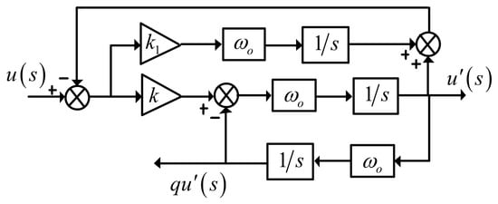
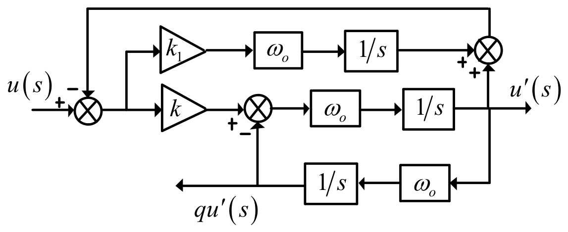
The TOGI structure adopted in this study is shown in Figure 1. It takes u(s) as its input and produces an in-phase output u′(s), and a quadrature output qu′(s). The corresponding transfer functions are expressed as follows:
Figure 1.
Block diagram of the TOGI.
Here, ωo denotes the resonant angular frequency of the TOGI, and k and k1 are the damping coefficient and dynamic tuning coefficient, respectively.
The pole–zero distribution of Equation (1) shows that D(s) has a double zero at the origin, whereas Q(s) has a single zero at the origin. Both channels therefore have zero gain at s = 0, enabling the rejection of input DC components. Compared with the conventional SOGI, the TOGI introduces zeros at the origin to prevent DC offsets from propagating to the outputs, thereby improving the robustness of synchronization signal extraction against DC offsets. Within the stable parameter region, k = 1.414 and k1 = 0.221 are selected according to the optimal pole-placement criterion proposed in [23], which requires all poles to have equal real parts. Unless otherwise stated, these parameter values are used throughout the subsequent analysis.
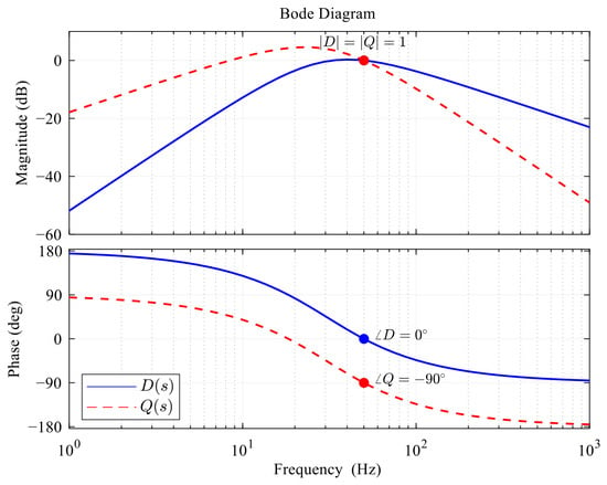
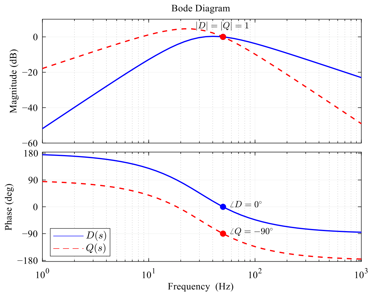
Figure 2 presents the magnitude and phase responses of D(s) and Q(s). At fo = 50 Hz both channels have unity gain and phases of 0° and −90°, respectively, so the TOGI produces two amplitude-matched signals in quadrature. Away from resonance their gains decrease, which provides selective extraction of the fundamental component and attenuation of low-frequency disturbances and higher-order harmonics; Q(s) is the exception, with a residual peak of about +4.6 dB near 23 Hz. This peak is a property of the third-order pole placement and does not materially alter the overall filtering behavior. In the positive-sequence extraction that follows, the outputs of the two channels are combined vectorially, and their contributions add as phasors rather than as magnitudes, so the residual peak of Q(s) is largely cancelled in the positive-sequence output, whose deviation from unity gain is much smaller than the peak of Q(s).
Figure 2.
Bode plots of D(s) and Q(s).
2.2. DTOGI-Based Positive-Sequence Extraction and Complex-Domain Modeling
Under unbalanced three-phase voltage conditions, the input voltages contain both fundamental positive- and negative-sequence components. To extract the fundamental positive-sequence component accurately, symmetrical component theory [24] is employed. The voltage components in the stationary αβ reference frame are cross-combined with the quadrature signals generated by the TOGIs to achieve sequence separation, as expressed in Equation (2).
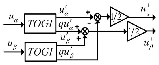
This method exploits the equivalent 90° phase displacement between the in-phase and quadrature outputs of each TOGI, together with appropriate weighting and cross-combination operations, to construct the fundamental positive-sequence component. The resulting filtering structure, consisting of two identical TOGIs and a positive-sequence extraction network, is referred to as the DTOGI. Its overall structure is shown in Figure 3.
Figure 3.
Overall block diagram of the DTOGI.
In Equation (2) uα and uβ denote the α- and β-axis voltage components obtained by applying the Clarke transformation to the three-phase grid voltages. DTOGI filtering and sequence separation yield output signals dominated by the fundamental positive-sequence component. Under nominal tuning conditions, DC offsets and the fundamental negative-sequence component are rejected by the corresponding zeros of the DTOGI transfer function, while other harmonics are attenuated according to its frequency response.
To provide a unified description of the DTOGI’s selectivity with respect to frequency and rotational direction, a complex-filter representation is introduced [25]. The voltage components in the αβ reference frame are expressed in complex form as
uαβ(s) = uα(s) + juβ(s)
Using the positive-sequence extraction relationship in Equation (2), the complex-domain transfer function of the DTOGI is obtained as follows:
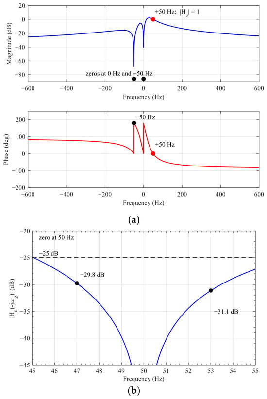
The numerator of Equation (4) indicates that Hc(s) has two zeros, located at s = 0 and s = −jωo. The zero at the origin corresponds to the zero-frequency DC offset component in the stationary αβ reference frame, whereas the zero at s = −jωo corresponds to the fundamental negative-sequence component at the resonant frequency, which rotates in the opposite direction to the positive-sequence component. Thus, when the actual grid angular frequency equals the resonant angular frequency, the DTOGI simultaneously rejects DC offsets and the fundamental negative-sequence component without requiring additional filters. Under this condition, the fundamental positive-sequence component is extracted without amplitude or phase distortion. The complex frequency response is shown in Figure 4.
Figure 4.
Magnitude and phase responses of Hc(s): (a) full range; (b) detail around −50 Hz, showing the negative-sequence gain |Hc(−jω)| between 45 and 55 Hz.
It should be noted that the rejection of the fundamental negative sequence described above holds only at the nominal frequency. When the grid frequency deviates to ωg, the negative-sequence component moves to s = −jωg and the zero no longer coincides with it, so the rejection becomes finite; the residual gain is
Figure 4b shows this gain between 45 and 55 Hz, a range that covers the frequency band permitted for 50 Hz supply systems by EN 50160. Within ±3 Hz of the nominal frequency the rejection remains better than 25 dB, and because the zero is of first order the attenuation deteriorates approximately linearly with the frequency deviation. The residual negative sequence appears in the dq frame as a ripple at 2ωg, which is well above the loop bandwidth and is therefore further attenuated by the loop.
As shown in Figure 3, the TOGI performs both quadrature signal generation and disturbance rejection. Unlike conventional frequency-adaptive SOGI or DSOGI structures, the proposed DTOGI prefilter has a resonant angular frequency fixed at the nominal value ωo, rather than updated in real time using the frequency estimated by the PLL. This arrangement avoids the additional dynamic coupling introduced by adaptive tuning of the resonant parameters. The complex frequency response in Figure 4 shows that, when the actual grid angular frequency ωg equals the fixed resonant angular frequency ωo, the DTOGI satisfies Hc(jωo) = 1, providing unity magnitude gain and zero phase shift for the fundamental positive-sequence component. However, when the grid frequency deviates from its nominal value, the complex gain Hc(jωg) departs from this ideal condition, introducing an overall amplitude gain error and a phase shift in the extracted fundamental positive-sequence vector. Accordingly, the following section derives closed-form expressions for these errors under frequency mismatch using the complex-domain transfer function of the DTOGI. A complex rotation compensation operator is then developed to provide unified correction of the amplitude and phase errors of the fundamental positive-sequence vector.
3. Complex Rotation Compensation Matrix and Its Implementation
The analysis in Section 2 shows that, when the actual grid angular frequency is equal to the resonant angular frequency of the DTOGI, the DTOGI extracts the fundamental positive-sequence component with unity magnitude gain and zero phase shift. However, under fixed-frequency operation, the actual grid frequency may deviate from its nominal value. Consequently, a frequency mismatch occurs between the grid fundamental component and the resonant frequency of the DTOGI. At this point, the complex gain of the DTOGI at the actual positive-sequence fundamental frequency deviates from unity, thereby introducing a magnitude-gain error and a phase shift.
The magnitude error and phase error correspond to the modulus and argument of the same complex gain, respectively. Therefore, they are not independent errors but two components of the same complex distortion. Accordingly, this section first analyzes the complex-frequency response of the fixed-frequency DTOGI under frequency mismatch and clarifies the coupling mechanism between the magnitude and phase errors. A complex rotation compensation operator is then constructed and transformed into a real-valued matrix suitable for digital implementation. Finally, the compensation characteristics and online implementation method are discussed.
3.1. Magnitude and Phase Errors Caused by Frequency Mismatch Under Fixed-Frequency Operation
By fixing the resonant angular frequency of the DTOGI at the nominal grid angular frequency ωo, a fixed-frequency DTOGI (FFDTOGI) is obtained. Unlike the frequency-adaptive DTOGI, the FFDTOGI does not use the frequency estimated by the PLL to update its resonant parameters online. Therefore, the additional frequency-feedback path introduced by resonant-frequency adaptation is eliminated, reducing the dynamic coupling between the filtering unit and the PLL as well as the associated potential stability risks. However, when the actual grid angular frequency ωg deviates from ωo, the fixed resonant frequency causes the DTOGI to produce a magnitude-gain error and a phase shift. Substituting s = jωg into (4) and rearranging yields the complex-frequency response of the FFDTOGI at the actual positive-sequence fundamental frequency:
where
Under normal grid operating conditions, k > 0, ωo > 0, and ωg > 0. Hence, the numerator of (5) is a positive real number. The magnitude and phase of (5) are therefore given by
Accordingly, the phase response of the filter can be expressed as
∠Hc(jωg) = −atan2(B,A)
The two-argument arctangent function, atan2(−B, A) = −atan2(B, A), is used instead of the single-argument arctangent function to avoid phase-quadrant ambiguity when the sign of A changes.
Equation (7a–d) show that the magnitude-gain error and phase shift are not independent distortions, but rather two representations of the same complex-frequency response. To further illustrate their geometric interpretation, let the fundamental positive-sequence voltage in the αβ stationary reference frame be represented by
where Um is the positive-sequence voltage magnitude and θ is its phase angle. The fundamental positive-sequence component at the output of the FFDTOGI is then
Equation (7a–d) shows that frequency mismatch causes both radial scaling and angular rotation of the output positive-sequence vector. The radial scaling is determined by ∣Hc(jωg)∣, whereas the angular rotation is determined by ∠Hc(jωg). Since both quantities originate from the same complex gain, the magnitude-gain error and phase shift are intrinsically coupled. This observation provides the theoretical basis for constructing the complex rotation–scaling compensation operator presented below.
3.2. Construction of the Complex Rotation Compensation Operator
According to (9), the magnitude-gain error and phase shift caused by frequency mismatch can be corrected simultaneously by cascading an appropriate complex compensation operator at the output of the FFDTOGI. The compensation operator is defined as
where Kc is the magnitude compensation coefficient and ϕc is the phase compensation angle. To ensure that the compensated FFDTOGI channel has unity gain and zero phase shift for the fundamental positive-sequence component, the following condition must be satisfied
Gc(ωg)Hc(jωg) = 1
It follows from (11) that
ϕc = atan2(B,A)
The corresponding trigonometric expressions are
Equations (12a,b) and (13a,b) show that the compensation angle has the opposite direction to the phase shift introduced by the filter. When ωg < ωo, B < 0, the filter phase is positive and the compensation angle is negative. When ωg > ωo, B > 0, the filter phase is negative and the compensation angle is positive. Thus, the compensation operator performs a reverse rotation to compensate for the phase shift caused by the frequency mismatch.
Combining (12a,b) and (13a,b), the complex compensation operator can be written as
As indicated by (14), the proposed compensation essentially inverts the complex gain at the fundamental positive-sequence frequency, rather than designing a dynamic inverse system for the entire filter transfer function. When the frequency estimate is accurate and the system is in sinusoidal steady state, the compensated positive-sequence vector has the same magnitude and phase as the ideal input positive-sequence vector. Therefore, both the fundamental positive-sequence magnitude-gain error and phase shift caused by frequency mismatch can be eliminated simultaneously.
3.3. Real-Time Implementation
For digital implementation, the complex compensation operation is expanded into the real domain. Define the uncompensated and compensated complex voltages as
uf = ufα + jufβ, uc = ucα + jucβ
According to uc = Gcuf, and using (14), the compensation operation can be expressed as
Equation (15) is the real-valued equivalent of the complex multiplication. The coefficient Kc corrects the radial deviation of the output vector, whereas the rotation matrix corrects its angular deviation. The two corrections are performed simultaneously through a two-dimensional matrix operation, while preserving the coupling between the α- and β-axis components. Under ideal compensation conditions, the compensated two-axis components recover their equal-amplitude orthogonal relationship.
To avoid the square-root, trigonometric, and inverse-trigonometric operations required by (12a,b) and (13a,b), the real and imaginary parts of the compensation matrix can be directly calculated from (14). Define
ωi denotes the angular-frequency estimate provided by the integral branch of the PLL PI regulator, which is used to replace the actual angular frequency ωg in (6a,b) and (14).
The real and imaginary parts of the complex compensation gain are then given by
Substituting (16a,b) into (16c,d) gives the following simplified expressions:
Equation (16f) indicates that the imaginary part of the compensation gain is directly proportional to the deviation of the estimated angular frequency from the nominal angular frequency, which facilitates rapid calculation in a digital controller.
Expanding the complex multiplication yields the following real-valued matrix operation:
Equations (16a–f) and (17) involve only addition, subtraction, multiplication, and division. No explicit calculation of Kc, ϕc, or the associated trigonometric functions is required. Therefore, the proposed method is suitable for real-time implementation on low-cost digital signal processors, microcontrollers, or field-programmable gate arrays.
In practical applications, the frequency estimate used by the compensation is ωi = ωo + Δω, where Δω is the output of the PI integral branch. To prevent integral windup and to keep the compensation denominator away from zero during start-up, abnormal frequency estimation or a voltage interruption, Δω is limited to [−0.9ωo, 0.9ωo], so that ωi remains within [0.1ωo, 1.9ωo]; the denominator of (16e) then stays above 5.5% of its nominal value and the coefficient magnitude does not exceed 2.9.
3.4. Compensation Characteristics and Overall PLL Implementation
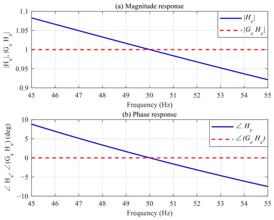
The following parameters are selected: k = 1.414, k1 = 0.221, ωo = 2π × 50 rad/s. The complex-frequency responses of the FFDTOGI before and after compensation are calculated over 45–55 Hz, a range that contains the 47–52 Hz permitted for 50 Hz supply systems by EN 50160, and are shown in Figure 5. Figure 5a presents the magnitude response and Figure 5b the phase response; the uncompensated response is Hc(jωg) and the compensated response is Gc(ωg)Hc(jωg).
Figure 5.
Comparison of the complex-frequency responses before and after compensation: (a) magnitude response; (b) phase response.
Before compensation, both the magnitude gain and the phase deviate from their ideal values as the grid frequency departs from nominal: at the lower and upper limits of the range, 47 and 52 Hz, the gain is 1.0494 and 0.9679, and the phase shift is +5.11° and −3.14°. When the compensation operator defined by (14) is applied, the theoretical response satisfies Gc(ωg)Hc(jωg) = 1, so the compensated gain is unity and the compensated phase shift is 0° over the whole range. These results verify the capability of the proposed complex compensation matrix to correct the magnitude and phase errors of the fundamental positive-sequence component simultaneously.
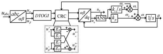
The overall structure of the proposed FFDTOGI-CRC-PLL is shown in Figure 6. First, the three-phase grid voltages are transformed into the αβ components using the Clarke transformation, and the FFDTOGI performs dc-offset suppression and fundamental positive-sequence extraction. Subsequently, the complex rotation–scaling compensation matrix defined in (17) corrects the magnitude and phase of the extracted fundamental positive-sequence voltage vector. The compensated voltage vector is transformed into the d- and q-axis components in the synchronous reference frame using the Park transformation. Amplitude normalization, PI loop filtering, and phase-angle integration are then performed to estimate the grid phase and frequency.
Figure 6.
Overall structure of the proposed FFDTOGI-CRC-PLL.
To reduce the influence of transient fluctuations in the proportional branch of the PI regulator on the compensation coefficients [14], the angular-frequency estimate ωi obtained from the integral branch is used to update gR and gI online according to (16e) and (16f), thereby ensuring smoother variations in the compensation coefficients. If the integral-branch output represents the angular-frequency deviation, the nominal angular frequency ωo must be added before calculating the compensation coefficients.
In addition, an amplitude normalization scheme (ANS) is introduced to normalize the q-axis voltage by the voltage-vector magnitude. This reduces the influence of voltage-magnitude fluctuations on the phase-detector gain and improves the robustness of phase locking.
In summary, the proposed FFDTOGI-CRC-PLL adopts a structure with fixed resonant parameters and output-side complex compensation. The FFDTOGI performs fundamental positive-sequence extraction and dc-offset suppression; the complex rotation compensation matrix corrects the magnitude and phase errors of the fundamental positive-sequence component caused by frequency mismatch; and the PLL tracks the grid phase and estimates the grid frequency. The resonant frequency of the DTOGI is held at the nominal value and is not updated from the frequency estimate, so the filter itself is independent of the estimate; the only quantity that varies with ωi is the compensation coefficient. That coefficient is a memoryless function of the estimate: it contains no integrator or delay, adds no state to the loop and leaves the order of the closed-loop system unchanged, and it reduces to the identity at the nominal operating point. The matrix is therefore intended to correct the complex gain of the extracted vector, not to reshape the dynamics of the DTOGI.
4. Small-Signal Modeling and Parameter Tuning
The overall structure of the proposed FFDTOGI-CRC-PLL is shown in Figure 6. The complex rotation compensation stage acts as a static algebraic element within the loop. Its coefficients are calculated using the frequency information provided by the integral branch of the PI controller. Therefore, this stage introduces no additional dynamic states and is algebraically coupled to the loop. Compared with the frequency-adaptive DTOGI, the fixed-frequency structure avoids the additional nonlinear terms associated with the time-varying ωi, as well as the parameter modulation caused by updating the resonant parameters using the estimated frequency. This simplifies small-signal modeling and controller design.
4.1. dq-Frame Model of the Prefilter
To facilitate small-signal analysis, the operating point is taken at the nominal frequency, so that ωi ≈ ωg ≈ ωo and θi ≈ θg. At this point the complex compensation matrix reduces to the identity, Gc(ωo) = 1/Hc(jωo) = 1, and the analysis below therefore addresses the dynamic relationship between the fixed-frequency DTOGI and the subsequent SRF-PLL.
To establish a unified loop model with the SRF-PLL, the complex transfer function in the stationary αβ reference frame must be transformed into the synchronous rotating dq reference frame. Following the complex-vector description of [25], the prefilter is represented in the αβ frame by Hc(s). Referring its output to the synchronous frame multiplies the signal by e−jθi, which, for a constant frame speed, corresponds to the frequency shift Hdq(s) = Hc(s + jωi) [25]. For a frequency-adaptive prefilter the coefficients of Hc depend on the estimated frequency ωi as well, so Hdq must itself be linearized about the operating point; in the proposed structure the resonant frequency is held at the nominal value ωo, so the coefficients are constant and Hdq is time-invariant. Taking the frame speed as ωo, the operating point about which the model is built gives
where
Separating Equation (18) into its real and imaginary parts gives
The input–output relationship of the DTOGI in the dq reference frame can then be expressed as
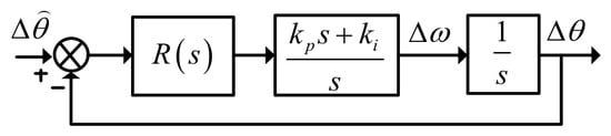
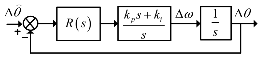
As indicated by Equation (21), the imaginary-part transfer function I(s) introduces cross-coupling between the d- and q-axes. This coupling can be understood as a rotation: the prefilter multiplies the voltage vector by a complex gain, whose magnitude changes the length of the vector and whose angle φ turns it. Within the low-frequency range considered in the PLL small-signal analysis, the influence of this cross-coupling on the system dynamics is generally limited. In particular, when the loop bandwidth is well below the grid fundamental frequency, the contribution of I(s) to the phase-detection channel can be neglected [26]. Accordingly, only the real-part transfer function R(s) is retained in the small-signal model, and the resulting simplified model is shown in Figure 7.
Figure 7.
Simplified small-signal model of the PLL.
4.2. Loop Model, Tuning and Parameter Sensitivity
Equation (20) shows that R(s) is a sixth-order real rational transfer function. Its direct inclusion in the PLL closed-loop analysis would result in a high-order characteristic equation, complicating parameter tuning and obscuring the dominant low-frequency dynamics. Following the model-order reduction approach for high-order PLL systems presented in [26], R(s) is approximated by a first-order lag element in the low-frequency range relevant to the loop dynamics,
where τ = 2/(kωo) is the equivalent time constant. Within this reduction, the value of τ is fixed by matching the low-frequency behavior of the dq-domain response: as s→0, Hdq(s) = 1/(1 + τs) + O(s2), so τ equals the initial slope of the phase response at the nominal frequency, |dφ/dω|. For a generalized integrator this slope is 2/kωo, because it is set by the damping term k rather than by the filter order, and the same constant appears in the small-signal model of the frequency-fixed SOGI-based PLL [14,26]. Because the match is made at low frequency, the reduction becomes progressively less accurate as the crossover frequency rises.
Substituting Equation (22) into the loop model shown in Figure 7 yields the small-signal open-loop transfer function of the PLL:
where kp and ki are the proportional and integral gains of the PI controller, respectively. As indicated by Equation (23), the proposed FFDTOGI-CRC-PLL can be approximated as a third-order type-II system under small-signal conditions. Compared with a conventional SRF-PLL, the additional dynamics introduced by the DTOGI are primarily represented by the equivalent time constant τ, which influences both the loop bandwidth and the damping characteristics.
To derive analytical tuning rules for the PLL controller, the extended symmetrical optimum (ESO) criterion is adopted to determine the PI gains [27]. The PI zero frequency and the equivalent DTOGI pole frequency are defined as ωz = ki/kp, ωp = 1/τ, respectively. Their relationship is specified as ωp = b2ωz, where b is a design parameter. By imposing the symmetrical frequency placement and unity-gain condition at the crossover frequency , the PI gains are obtained as
Under this tuning criterion, the phase margin is primarily determined by the design parameter b. The corresponding values of kp, ki, and ωc for different choices of b are summarized in Table 1.
Table 1.
PI gains and performance for different b values.
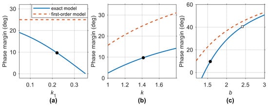
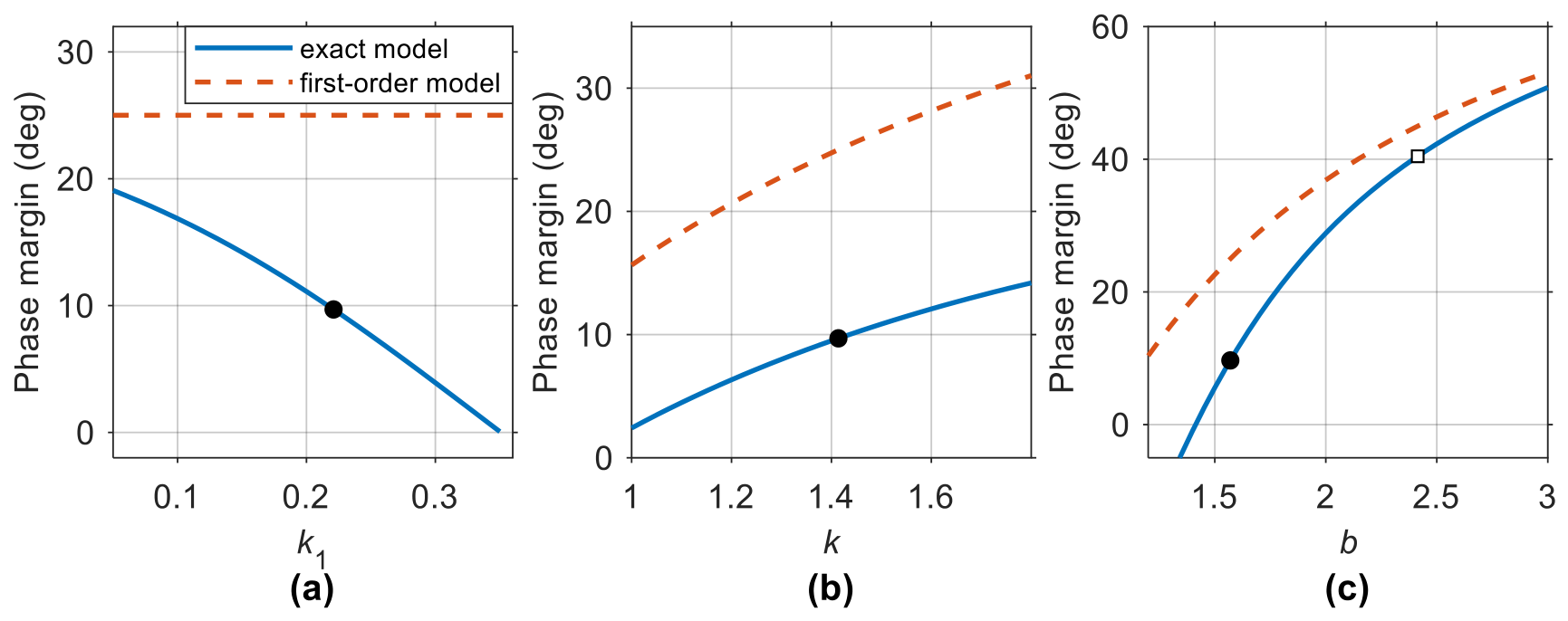
The fifth column of Table 1 gives the margins of the reduced model used for the tuning; the sixth gives the values obtained with the exact model. When k or k1 departs from its nominal value, the margin changes further. The PI gains are fixed by (24), so their influence is already contained in that margin and they are not varied separately. Of the prefilter parameters, only k enters (22) and hence the tuning; k1 does not appear in (22), yet it shifts the poles of R(s). As shown in Figure 8a, the exact margin falls from 16.8° to 3.9° as k1 increases from 0.10 to 0.30, whereas the first-order model remains at 25.0° throughout. The reduced model is thus completely insensitive to k1, so its effect can only be captured by the exact model. This trend also explains why k1 cannot be made large: it sets the decay rate of the dc component, so a larger value rejects the dc offset faster but lowers the margin, and 0.221 is adopted here as a compromise between the two.
Figure 8.
Phase margin versus the prefilter parameter k1 (a) and k (b), and versus the design parameter b (c), computed with the exact model (solid) and the first-order equivalent (dashed). The filled marker denotes the design point k1 = 0.221, k = 1.414, b = 1.570; the open square in (c) marks b = 2.414.
Figure 8b gives the margin as a function of k: as k increases from 1.0 to 1.8 the exact margin rises from 2.4° to 14.2°, because τ is inversely proportional to k. Figure 8c gives the margin as a function of the design parameter b: between b = 1.2 and b = 3.0 the exact margin rises from a negative value to 50.8°, while the first-order model overestimates it by 3–13°, the overestimate being largest on the low-b (high-bandwidth) side. The settings b = 2.414 and b = 1.570 used in this paper form a low- and a high-bandwidth pair, with margins of 40.5° and 9.7°, respectively; although the lower margin is small, it remains within the stable range, and it is mainly at this operating point that the difference between the fixed- and frequency-adaptive structures is manifested.
4.3. Accuracy of the Model and Its Validation
The accuracy of the reduced model is assessed in two steps. It is compared first with the exact sixth-order transfer function that it replaces, and then with a time-domain simulation of the complete PLL.
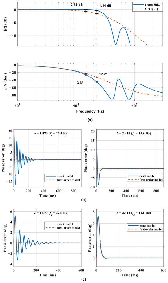
The reduction is assessed in Figure 9a, where R(jω) is compared with the first-order equivalent 1/(1 + jωτ) in a Bode plot and the resulting phase error is plotted on the same axes. At the lower bandwidth (b = 2.414, fc = 14.6 Hz) the phase discrepancy is 3.6° and the magnitude discrepancy 0.73 dB, so that the margin of 45.0° predicted by (23) becomes 40.5° with the exact model; at the higher bandwidth (b = 1.570, fc = 22.5 Hz) the discrepancy grows to 12.2° and 1.14 dB, the margin falls from 25.0° to 9.7°, and the crossover frequency moves from 22.5 to 24.5 Hz. The reduction can therefore be used directly for tuning when fc ≤ 15 Hz, where the phase error stays within 5°, whereas a higher bandwidth requires the margin to be verified with the exact model.
Figure 9.
Accuracy of the reduced-order model: (a) Bode plots of R(jω) and of the first-order equivalent; phase-error responses to (b) a 20° phase step and (c) a 2 Hz frequency step, at b = 1.570 (left) and b = 2.414 (right).
The same difference appears in the time domain. Figure 9b compares the closed-loop phase-error responses of the two models to a 20° phase step, and Figure 9c those to a 2 Hz frequency step. For the 20° step the negative overshoot of the exact model reaches 17.3°, against 11.9° for the first-order model; for the 2 Hz step the peak phase errors are 5.19° and 4.69°, and the oscillations of the exact model decay more slowly. At b = 2.414 the same comparison gives 8.94° against 6.71° for the step and 7.21° against 6.74° for the ramp, with the absolute deviation being smaller although the relative one is comparable. The reduction thus overestimates both the phase margin and the damping, consistently with the phase discrepancy of Figure 9a.
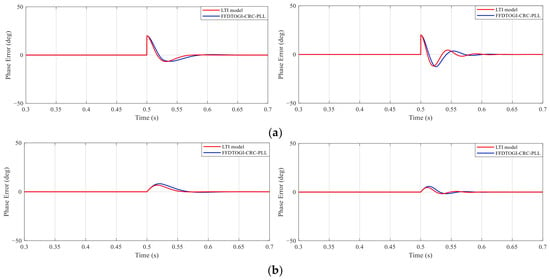
The second check compares the linear model with a time-domain simulation of the complete PLL. The simulation is built in Simulink with the DTOGI implemented from its state equations, the compensation coefficients updated at every sampling instant and the PI regulator running at 10 kHz. Under the 20° phase step and the 2 Hz frequency step of Figure 10 the two responses have the same shape and settle at the same time, but the linearized model underestimates the negative overshoot by about 10%. This is expected once the perturbation is no longer small. The reduction holds only while fc ≪ fo and the perturbation remains small, limits quantified in Figure 9 and Table 1, and in Figure 10, respectively. It serves only to obtain the initial tuning from (24); every margin quoted here is computed with the exact model, and the approximation is not applied beyond the validated bandwidth.
Figure 10.
Phase-error response of the linearized model (red) and of the complete nonlinear model (blue) under (a) a 20° phase step and (b) a 2 Hz frequency step, for b = 1.570 (left) and b = 2.414 (right).
5. Experimental Results and Discussion
5.1. Experimental Setup and Methodology
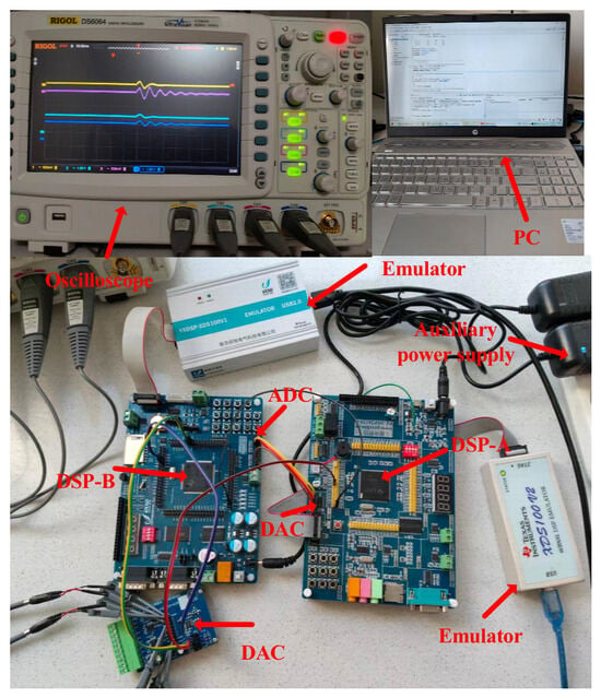
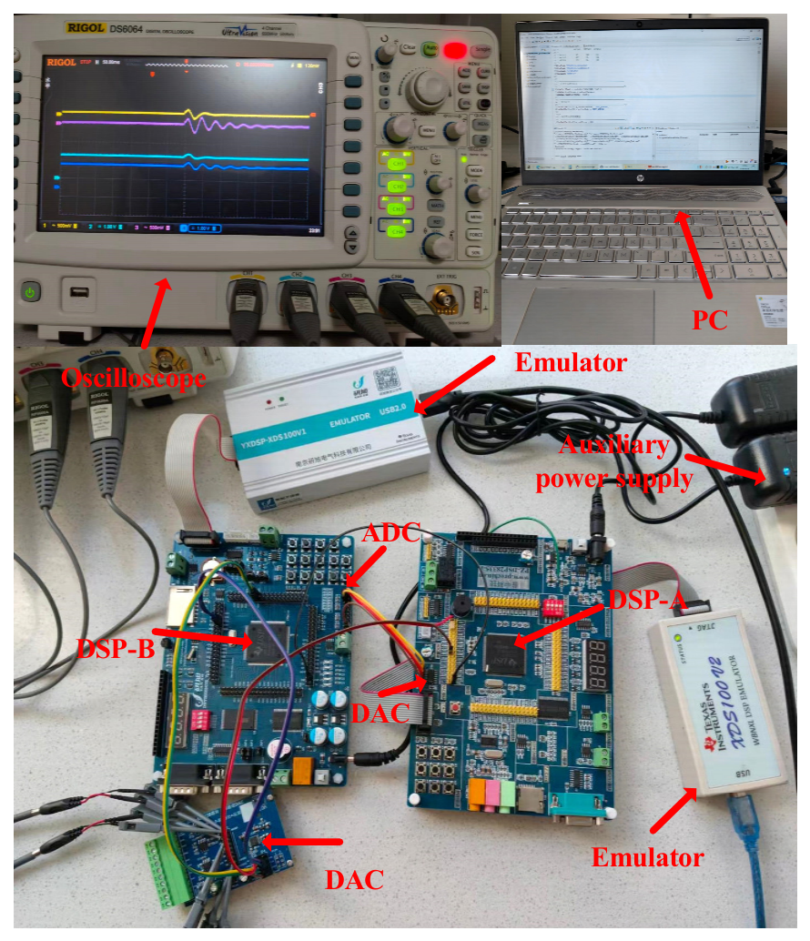
To validate the dynamic response and DC-offset rejection capability of the proposed FFDTOGI-CRC-PLL, a digital signal processor (DSP)-based experimental platform was developed, as shown in Figure 11. The platform consists of two TMS320F28335 DSPs. DSP A generates three-phase voltage signals through a digital-to-analog converter (DAC) to emulate grid voltages. DSP B acquires these signals through an analog-to-digital converter (ADC) and executes the PLL algorithms in real time. The phase-estimation errors and estimated frequencies are then output through a DAC for experimental observation. The sampling frequency is set to 10 kHz. The platform is therefore signal-level: the voltages are generated and acquired digitally, and no converter or grid impedance is involved.
Figure 11.
Experimental setup.
Two sets of comparative experiments were conducted to evaluate the dynamic performance and disturbance rejection capability of the proposed method.
- (1)
- In the first set, the frequency-adaptive DTOGI-PLL(FADTOGI-PLL) was selected as the benchmark. Its structure is derived from the mixed second- and third-order generalized integrator PLL (MSTOGI-PLL) reported in [21] and extended in this study to a dual third-order generalized integrator configuration. The proposed method and the FADTOGI-PLL use identical proportional–integral (PI) controller parameters for each parameter setting, as listed in Table 1. Two settings, b = 2.414 (fc = 14.6 Hz) and b = 1.570 (fc = 22.5 Hz), corresponding to lower and higher control bandwidths, respectively, were considered. The fixed-frequency and frequency-adaptive structures were compared in terms of settling time, maximum transient deviation, and oscillation decay under frequency steps, phase jumps, and combined disturbances.
- (2)
- In the second set, the fixed-frequency DSOGI-PLL (FFDSOGI-PLL) reported in [14] was selected as the benchmark to assess filtering performance and phase-estimation accuracy under combined voltage disturbances, including DC offsets and voltage sags. The proposed FFDTOGI-CRC-PLL uses the PI controller parameters corresponding to b = 1.570 in Table 1. For the FFDSOGI-PLL, kp ≈ 150.0 and ki ≈ 11,244 were selected according to the tuning procedure in [14]. Both methods use the same sampling frequency and nominal grid frequency, with comparable control bandwidths, to ensure a fair comparison.
Five disturbance cases were designed to evaluate operation under different grid conditions, as summarized in Table 2.
Table 2.
Experimental disturbance cases.
The counts in Table 3 refer to the correction stage only—the complex-gain evaluation of (16e,f), the resonator retuning of the FADTOGI-PLL and the magnitude-and-phase correction of the FFDSOGI-PLL. The times were measured by toggling a general-purpose output at the entry and exit of the interrupt and reading the pulse width, which equals the execution time of the interrupt body. The three structures agree within 1.2 µs: the proposed correction is 1.2 µs slower than the resonator retuning because of its eight additional multiplications, and it matches the SOGI correction, whose two transcendental calls are offset by a prefilter of one order lower. The proposed method is therefore no more than 1.2 µs slower than either benchmark, so its improvement in dynamic performance is obtained without a significant penalty in execution time.
Table 3.
Computational cost of the correction stage of the three structures, per sampling period.
5.2. Dynamic Performance
The indicators used in Table 4 and Table 5 are defined as follows. The phase error is εθ = θ − θref, where θref is the phase of the voltage generated by DSP A and is therefore known before the DAC; the frequency error is εf = f − fref. The settling time is the interval after which |εf| < 0.4 Hz and |εθ| < 4° hold continuously for at least 20 ms. The maximum frequency overshoot is the largest |εf| within 200 ms of the disturbance, and the steady-state ripple is the peak-to-peak value measured over the 0.5–1.0 s window that follows it.
Table 4.
Quantitative results for the first set of comparative experiments.
Table 5.
Quantitative results for the second set of comparative experiments.
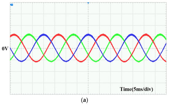
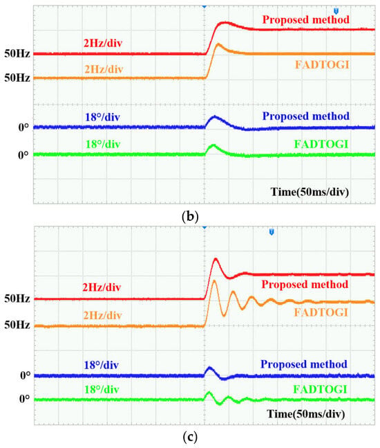
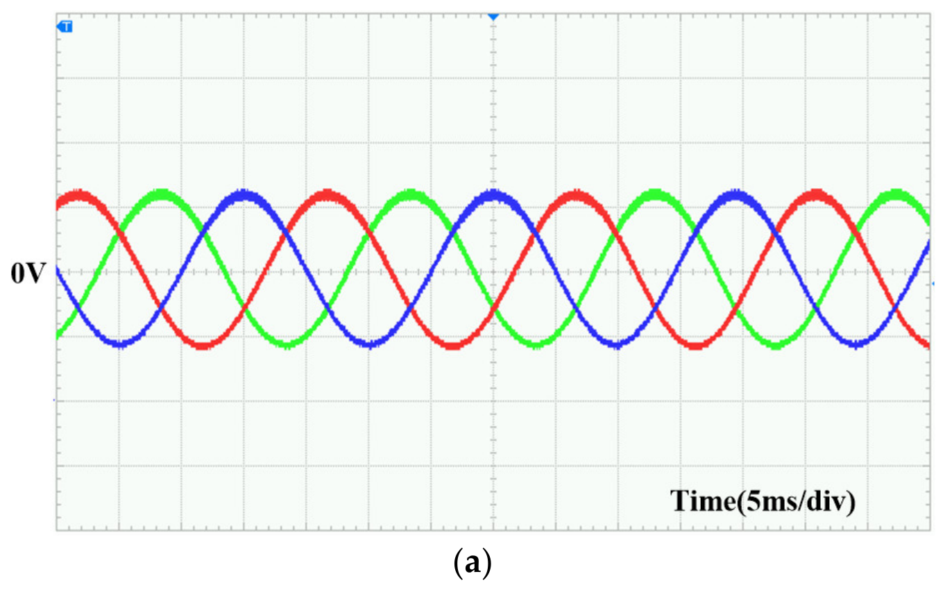
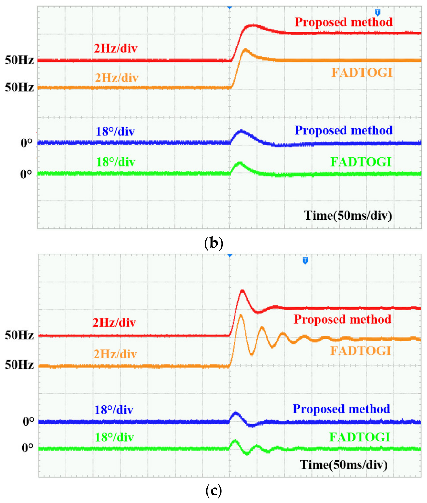
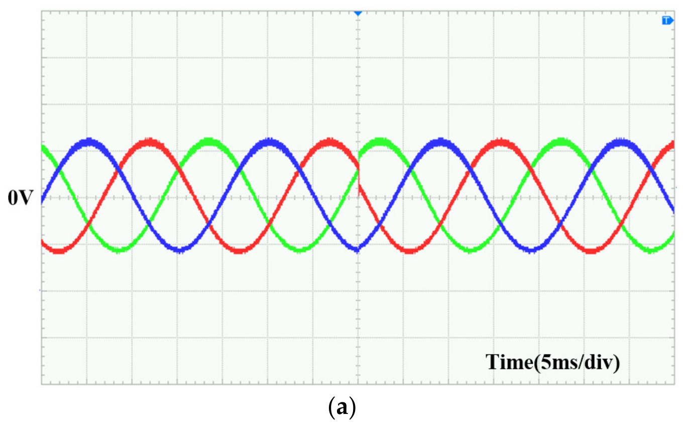
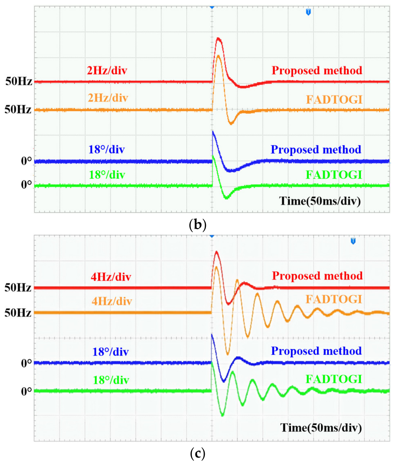
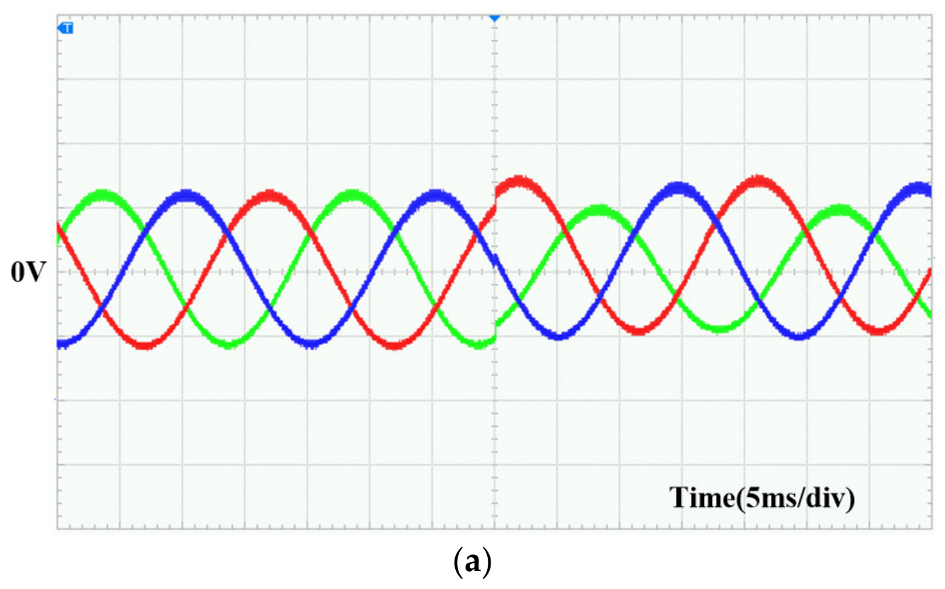
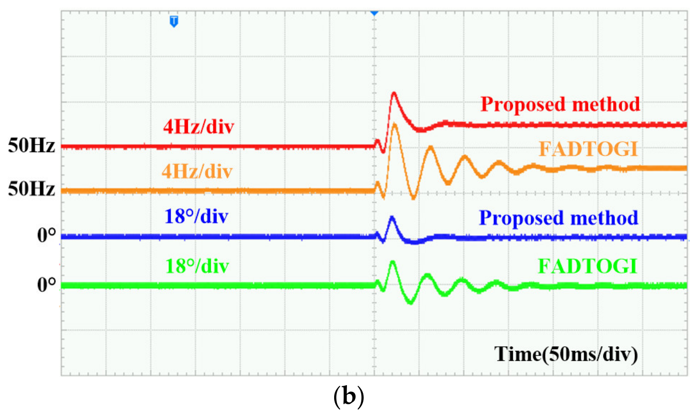
As shown in Figure 12, under the lower-bandwidth setting, both methods track the frequency step and converge to the new steady-state value after some overshoot. Their overall dynamic responses are similar, and neither exhibits pronounced, prolonged oscillatory transients. Under the higher-bandwidth setting, however, the differences become more evident. The estimated frequency and phase-estimation error of the FADTOGI-PLL exhibit pronounced decaying oscillations over multiple cycles, resulting in a longer settling process, whereas the proposed FFDTOGI-CRC-PLL exhibits only small, rapidly decaying transient fluctuations and reaches steady state more quickly.
Figure 12.
Experimental results for Case 1: (a) three-phase grid voltages; (b) estimated frequencies and phase-estimation errors for b = 2.414; (c) estimated frequencies and phase-estimation errors for b = 1.570.
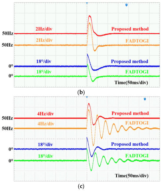
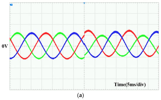
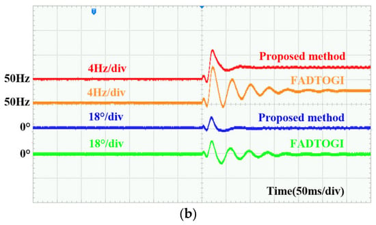
As shown in Figure 13, both methods track the phase jump under the lower-bandwidth setting, with broadly similar dynamic responses. The proposed method exhibits a slightly longer settling time than the FADTOGI-PLL but a smaller transient frequency deviation. Under the higher-bandwidth setting, the phase-estimation transient of the FADTOGI-PLL becomes substantially longer and is accompanied by prolonged decaying oscillations. In contrast, the proposed FFDTOGI-CRC-PLL settles more quickly following the phase jump, with faster attenuation of the transient oscillations.
Figure 13.
Experimental results for Case 2: (a) three-phase grid voltages; (b) estimated frequencies and phase-estimation errors for b = 2.414; (c) estimated frequencies and phase-estimation errors for b = 1.570.
As shown in Figure 14, when the frequency step and combined voltage disturbances are applied simultaneously, the FADTOGI-PLL exhibits pronounced transient fluctuations in both the estimated frequency and phase-estimation error, together with long-lasting decaying oscillations. In contrast, the proposed FFDTOGI-CRC-PLL exhibits a smoother transient response, with faster attenuation of the fluctuations and a shorter settling process.
Figure 14.
Experimental results for Case 3: (a) three-phase grid voltages; (b) estimated frequencies and phase-estimation errors for b = 1.570.
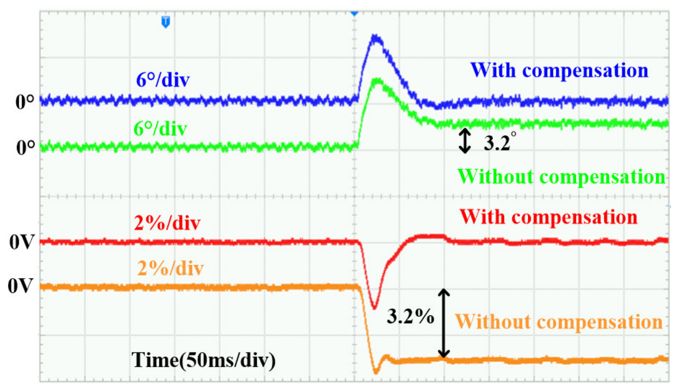
In Figure 15 the compensation matrix of one of two otherwise identical instances is replaced by the identity. After the 2 Hz step the uncompensated instance retains a 3.2° phase offset and a 3.2% magnitude error, whereas the compensated instance settles within 0.1° and 0.1%. These residuals agree with the 3.14° and 3.21% predicted by (7d) and (7a) at 52 Hz. The improvement of Cases 1–3 therefore comes from the compensation itself, not from a different loop gain.
Figure 15.
Effect of the compensation under a 2 Hz frequency step.
The results in Figure 12, Figure 13, Figure 14 and Figure 15 and Table 4 show that, under the higher-bandwidth setting, the FADTOGI-PLL exhibits pronounced multicycle decaying oscillations and substantially longer settling times across all three disturbance cases. By comparison, the proposed FFDTOGI-CRC-PLL exhibits smoother transients and faster oscillation decay, indicating greater dynamic robustness to the tested bandwidth settings and combined disturbances.
These observations are consistent with the theoretical analysis. In the FADTOGI-PLL, the estimated frequency is used to update the resonant parameters online, introducing an additional dynamic coupling path between the filter parameters and frequency estimation. As the control bandwidth increases, this parameter modulation increasingly affects the closed-loop pole locations, leading to dynamic behavior associated with reduced effective damping. Consequently, more pronounced oscillations and longer settling times may occur.
In contrast, the proposed method uses fixed resonant parameters. Although the complex rotation compensation coefficients are updated online using the estimated frequency, they do not modify the resonant parameters of the DTOGI. This eliminates the parameter-modulation path from the estimated frequency to the filter resonance characteristics. The method therefore compensates for frequency-deviation-induced magnitude and phase errors while keeping the DTOGI filter dynamics relatively independent of the frequency-estimation loop, resulting in faster transient convergence and improved oscillation suppression under the tested conditions.
5.3. Steady-State Accuracy and Spectral Analysis
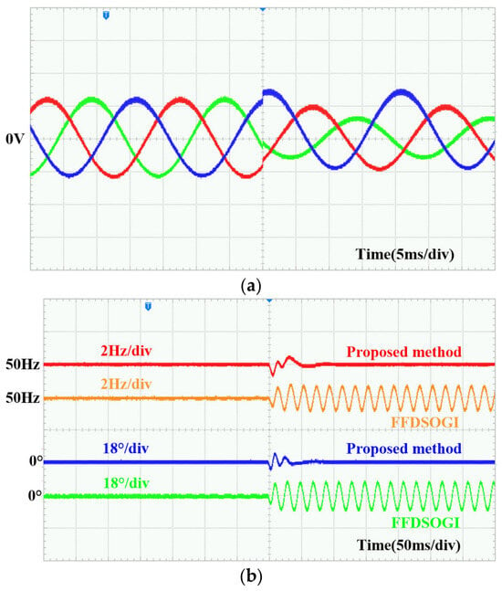
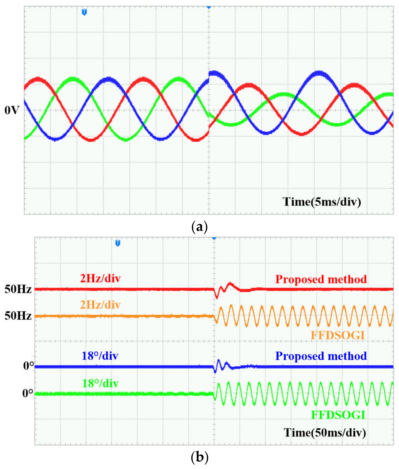
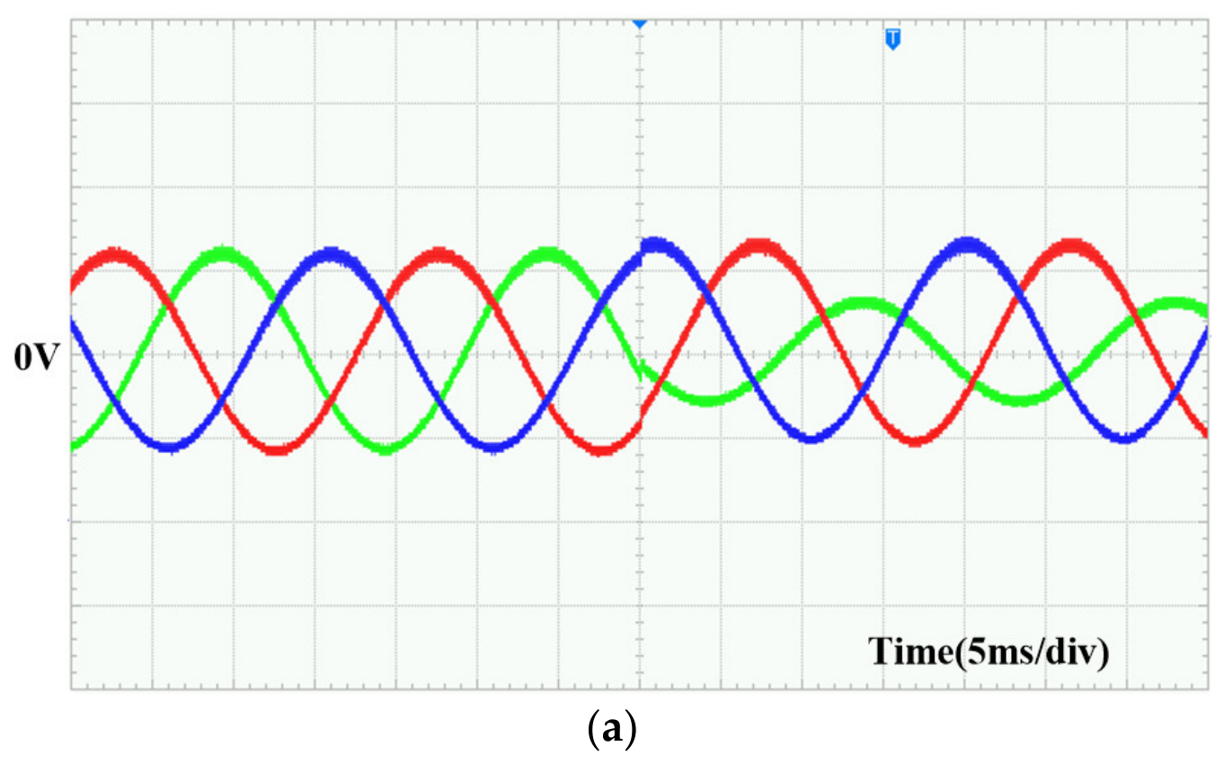
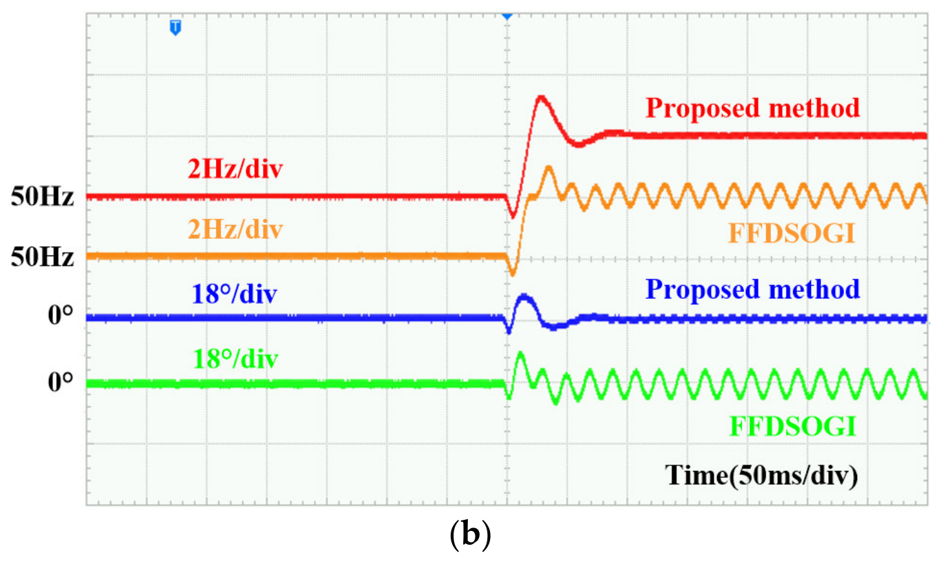
As shown in Figure 16, both methods maintain stable frequency and phase estimates before the disturbances are applied. Following disturbance application, the proposed FFDTOGI-CRC-PLL returns to steady state after a brief transient, with no noticeable steady-state ripple in either the estimated frequency or phase-estimation error. In contrast, the FFDSOGI-PLL exhibits sustained periodic fluctuations in both signals, indicating a noticeable degradation in steady-state estimation accuracy.
Figure 16.
Experimental results for Case 4: (a) three-phase grid voltages; (b) estimated frequencies and phase-estimation errors.
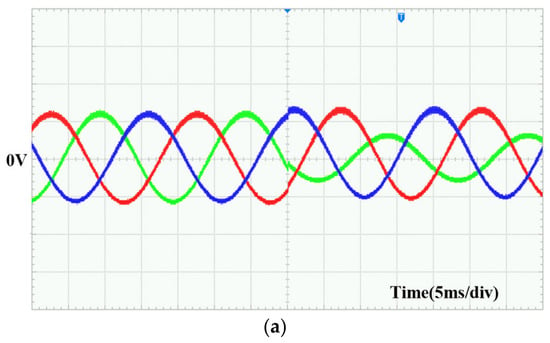
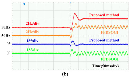
As shown in Figure 17, the proposed FFDTOGI-CRC-PLL tracks the new grid frequency following disturbance application. The transient fluctuations decay rapidly, and the phase-estimation error subsequently settles without sustained oscillations or divergence. In contrast, the FFDSOGI-PLL exhibits pronounced, sustained periodic oscillations in both the estimated frequency and phase-estimation error after the frequency step, indicating substantially degraded steady-state estimation performance under this disturbance condition.
Figure 17.
Experimental results for Case 5: (a) three-phase grid voltages; (b) estimated frequencies and phase-estimation errors.
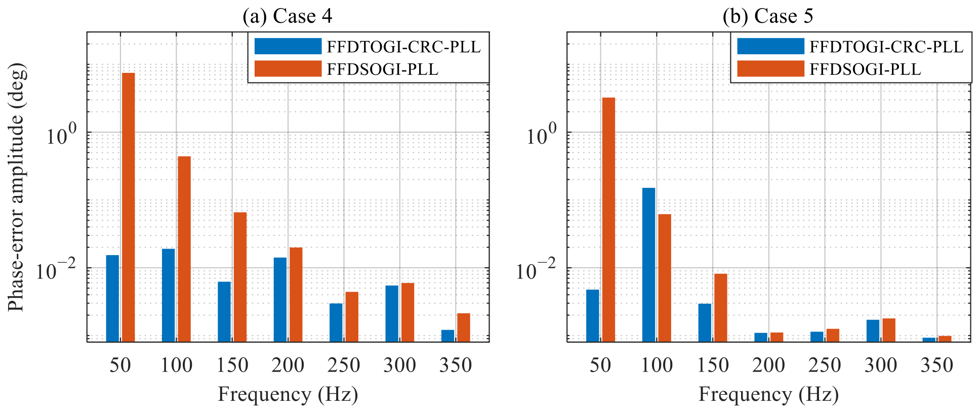
The residual oscillation of Figure 16 and Figure 17 is quantified in Figure 18. In Case 4 the residual of the FFDSOGI-PLL is dominated by the fundamental, 7.48°, against 0.015° for the proposed method, a difference of 54 dB; in Case 5 the benchmark retains 3.24° while the proposed method falls to 0.005°, its largest component moving to the second harmonic at 0.15°. From the third harmonic upwards both methods stay below 0.05°.
Figure 18.
Harmonic spectrum of the phase-error signal in (a) Case 4 and (b) Case 5.
The dc offsets appear as a fundamental ripple because the offsets of the three channels are not equal and therefore do not cancel in the Clarke transform, leaving a constant vector in the αβ frame that rotates at −ω in the synchronous frame. The SOGI passes it to its quadrature output, whose gain at zero frequency is non-zero, whereas the proposed structure rejects it through the zeros of both integrator outputs at the origin.
Taken together, Figure 16 and Figure 17 and Table 5 show that the proposed FFDTOGI-CRC-PLL maintains stable phase locking under the tested combinations of voltage unbalance and DC offsets, including the case with an additional frequency step. These results further demonstrate its steady-state disturbance rejection capability under combined voltage disturbances involving DC offsets. It should be noted, however, that the negative-sequence attenuation analysed in Section 2.2 is not verified here, since only the frequency and phase errors are recorded; Cases 3–5 exercise it only indirectly.
These experimental observations are consistent with the theoretical analysis. The relevant output channels of the third-order generalized integrator used in the proposed method have zero gain at s = 0, thereby rejecting the steady-state transmission of DC components to the quadrature-signal generation and subsequent phase-detection stages. In contrast, the quadrature output channel of the second-order generalized integrator has a nonzero DC gain, allowing DC components to propagate to its output and produce sustained oscillations in the frequency and phase estimates. Furthermore, under frequency-step conditions, complex rotation compensation corrects the magnitude and phase errors introduced by the fixed-frequency filter. The proposed method thus preserves its DC-offset rejection capability while retaining frequency-tracking capability.
6. Conclusions
This paper proposes a fixed-frequency dual third-order generalized integrator phase-locked loop with complex rotation compensation (FFDTOGI-CRC-PLL). The proposed method combines fixed-frequency prefiltering with complex-domain magnitude and phase compensation, thereby improving the PLL’s tolerance to dc offset and frequency deviations without adjusting the resonant frequency of the DTOGI. Experimental results demonstrate that, under the investigated nonideal operating conditions, the proposed FFDTOGI-CRC-PLL exhibits smaller transient oscillations and better stable-operating performance than the FADTOGI-PLL when operating with a high bandwidth. Compared with the FFDSOGI-PLL, the proposed method significantly reduces the steady-state phase-angle error under three-phase voltage dc-offset and compound-disturbance conditions.
The experimental results also verify the effectiveness of the DTOGI in blocking dc components and the capability of the complex compensation scheme to correct the fundamental-frequency magnitude and phase errors caused by the frequency mismatch of the fixed-frequency filter. Consequently, the proposed PLL maintains accurate phase and frequency tracking under different disturbance conditions. These results indicate that disturbance rejection in the prefilter and fundamental-component magnitude–phase correction can be designed as relatively independent functional modules and coordinated through a unified complex-domain representation, providing a feasible solution for the design of fixed-frequency three-phase PLLs.
Three limitations qualify these results. The validation is signal-level and does not cover the power stage, the grid impedance, harmonic distortion or multi-converter operation. Harmonic rejection is set by the prefilter alone, and the compensation, being a constant complex gain, leaves the relative attenuation unchanged; complete suppression is therefore not claimed. Between 15 and 40 Hz the positive-sequence gain of the prefilter exceeds unity by up to 2.1 dB, so inter-harmonics in that band are attenuated less than the higher harmonics. The small-signal model takes the compensation matrix as the identity at the operating point, so the effect of the coefficient update on the loop dynamics is not represented in it, and characterising that effect is left for future work. Future work will also address digital control delays and operation under multiple simultaneous disturbances.
Author Contributions
Conceptualization, L.J. and X.L.; methodology, L.J. and P.J.; software, L.J.; validation, L.J. and X.L.; formal analysis, L.J.; investigation, P.J.; resources, P.J. and H.Y.; data curation, X.L.; writing—original draft preparation, L.J.; writing—review and editing, X.L. and H.Y.; visualization, P.J.; supervision, P.J.; project administration, X.L. and H.Y.; funding acquisition, X.L. All authors have read and agreed to the published version of the manuscript.
Funding
This research was funded by the Science and Technology Research Project of Henan Province, grant number 252102240115; the Scientific Research Project Cultivation Fund of Anyang Institute of Technology, grant number YPY2024002; and the Key Laboratory of New Energy Power Systems, Anyang Institute of Technology, grant number SYS202402.
Data Availability Statement
The original contributions presented in this study are included in the article. Further inquiries can be directed at the corresponding author.
Acknowledgments
The authors gratefully acknowledge the support provided by the Key Discipline of Henan Province (“Electronic Information”).
Conflicts of Interest
The authors declare no conflicts of interest.
Abbreviations
The following abbreviations are used in this manuscript:
| PLL | phase-locked loop |
| SRF-PLL | synchronous reference frame phase-locked loop |
| CRC | complex rotation compensation |
| DC | direct current |
| DSP | digital signal processor |
| SOGI | second-order generalized integrator |
| DSOGI | double second-order generalized integrator |
| FADTOGI-PLL | frequency-adaptive dual third-order generalized integrator phase-locked loop |
| FFDSOGI-PLL | fixed-frequency double second-order generalized integrator phase-locked loop |
| TOGI | third-order generalized integrator |
| DTOGI | dual third-order generalized integrator |
| FFDTOGI | fixed-frequency dual third-order generalized integrator |
| FFDTOGI-CRC-PLL | frequency-fixed dual third-order generalized integrator PLL with complex rotation compensation |
References
- Golestan, S.; Guerrero, J.M.; Vasquez, J.C. Three-phase PLLs: A review of recent advances. IEEE Trans. Power Electron. 2017, 32, 1894–1907. [Google Scholar] [CrossRef] [Scilit]
- Golestan, S.; Guerrero, J.M.; Vasquez, J.C. Single-phase PLLs: A review of recent advances. IEEE Trans. Power Electron. 2017, 32, 9013–9030. [Google Scholar] [CrossRef] [Scilit]
- Xu, J.; Qian, H.; Hu, Y.; Bian, S.; Xie, S. Overview of SOGI-based single-phase phase-locked loops for grid synchronization under complex grid conditions. IEEE Access 2021, 9, 39275–39291. [Google Scholar] [CrossRef] [Scilit]
- Zhou, J.; Wang, E.; Xu, J.; Yu, Y. Robust detection algorithm for single-phase voltage sags integrating adaptive composite morphological filtering and improved MSTOGI-PLL. Energies 2026, 19, 1621. [Google Scholar] [CrossRef] [Scilit]
- Golestan, S.; Ramezani, M.; Guerrero, J.M.; Freijedo, F.D.; Monfared, M. Moving average filter based phase-locked loops: Performance analysis and design guidelines. IEEE Trans. Power Electron. 2014, 29, 2750–2763. [Google Scholar] [CrossRef] [Scilit]
- Zhu, Y.; Yu, J.; Luo, C.; Zhou, Y.; Wang, X.; Li, G.; Dai, Z. An enhanced CDSC-based grid parameter estimation method for distorted grids. Energies 2026, 19, 3868. [Google Scholar] [CrossRef] [Scilit]
- Khazraj, H.; da Silva, F.F.; Bak, C.L.; Golestan, S. Analysis and design of notch filter-based PLLs for grid-connected applications. Electr. Power Syst. Res. 2017, 147, 62–69. [Google Scholar] [CrossRef] [Scilit]
- Zhang, C.; Chen, J.; Si, W. Analysis of phase-locked loop filter delay on transient stability of grid-following converters. Electronics 2024, 13, 986. [Google Scholar] [CrossRef] [Scilit]
- Nguyen, A.T.; Lee, D.-C. Advanced grid synchronization scheme based on dual eSOGI-FLL for grid-feeding converters. IEEE Trans. Power Electron. 2022, 37, 7218–7229. [Google Scholar] [CrossRef] [Scilit]
- Ramezani, M.; Golestan, S.; Li, S.; Guerrero, J.M. A simple approach to enhance the performance of complex-coefficient filter-based PLL in grid-connected applications. IEEE Trans. Ind. Electron. 2018, 65, 5081–5085. [Google Scholar] [CrossRef] [Scilit]
- Zhang, C.; Føyen, S.; Suul, J.A.; Molinas, M. Modeling and analysis of SOGI-PLL/FLL-based synchronization units: Stability impacts of different frequency-feedback paths. IEEE Trans. Energy Convers. 2021, 36, 2047–2058. [Google Scholar] [CrossRef] [Scilit]
- Lei, J.; Quan, X.; Feng, S.; Zhao, J.; Chen, W. Accurate modeling of PLL with frequency-adaptive prefilter: On the positive feedback effect. IEEE Trans. Power Electron. 2022, 37, 3747–3752. [Google Scholar] [CrossRef] [Scilit]
- Xiao, F.; Dong, L.; Li, L.; Liao, X. A frequency-fixed SOGI-based PLL for single-phase grid-connected converters. IEEE Trans. Power Electron. 2017, 32, 1713–1719. [Google Scholar] [CrossRef] [Scilit]
- Hoepfner, B.; Vick, R. A three-phase frequency-fixed DSOGI-PLL with low computational effort. IEEE Access 2023, 11, 34932–34941. [Google Scholar] [CrossRef] [Scilit]
- Gautam, S.; Xiao, W.; Lu, D.D.-C.; Ahmed, H.; Guerrero, J.M. Development of frequency-fixed all-pass filter-based single-phase phase-locked loop. IEEE J. Emerg. Sel. Top. Power Electron. 2022, 10, 506–517. [Google Scholar] [CrossRef] [Scilit]
- Li, J.; Wang, Q.; Xiao, L.; Lu, Y.; Wu, Q. Analysis and improvement of fourth-order generalised integrator based phase-locked loop. IET Power Electron. 2021, 14, 386–396. [Google Scholar] [CrossRef] [Scilit]
- EN 50160; Voltage Characteristics of Electricity Supplied by Public Electricity Networks. European Committee for Electrotechnical Standardization (CENELEC): Brussels, Belgium, 2010.
- GB/T 19964; Technical Requirements for Connecting Photovoltaic Power Station to Power Systems. Standardization Administration of China: Beijing, China, 2012.
- Guo, L.; Ye, Q.; Jin, N.; Li, Y.; Wu, Z. A three-phase phase-locked loop design method based on improved frequency-fixed DSOGI and cross-compensation. Power Syst. Prot. Control 2024, 52, 133–142, (In Chinese with English abstract). [Google Scholar]
- Smadi, I.A.; Albatran, S.; Fawaz, B.B.; Ali, M.S. DC offset rejection and harmonics filtering improvement in second-order generalized integrator based-phase-locked loop: A comprehensive review. Renew. Sustain. Energy Rev. 2025, 220, 115891. [Google Scholar] [CrossRef] [Scilit]
- Zhang, C.; Zhao, X.; Wang, X.; Chai, X.; Zhang, Z.; Guo, X. A grid synchronization PLL method based on mixed second- and third-order generalized integrator for DC-offset elimination and frequency adaptability. IEEE J. Emerg. Sel. Top. Power Electron. 2018, 6, 1344–1356. [Google Scholar] [CrossRef] [Scilit]
- Hui, N.; Wang, D.; Li, Y. An efficient hybrid filter-based phase-locked loop under adverse grid conditions. Energies 2018, 11, 703. [Google Scholar] [CrossRef] [Scilit]
- Hui, N.; Wu, B.; Han, X. Grid synchronization method based on three novel types of third-order generalized integrators. Comput. Electr. Eng. 2024, 117, 109257. [Google Scholar] [CrossRef] [Scilit]
- Golestan, S.; Monfared, M.; Freijedo, F.D.; Guerrero, J.M. Dynamics assessment of advanced single-phase PLL structures. IEEE Trans. Ind. Electron. 2013, 60, 2167–2177. [Google Scholar] [CrossRef] [Scilit]
- Li, W.; Ruan, X.; Bao, C.; Pan, D.; Wang, X. Grid Synchronization Systems of Three-Phase Grid-Connected Power Converters: A Complex-Vector-Filter Perspective. IEEE Trans. Ind. Electron. 2014, 61, 1855–1870. [Google Scholar] [CrossRef] [Scilit]
- Golestan, S.; Akhavan, A.; Vasquez, J.C. On small-signal modelling of advanced phase-locked loops for three-phase grid-connected applications. In Proceedings of the 2024 IEEE International Conference on Environment and Electrical Engineering and 2024 IEEE Industrial and Commercial Power Systems Europe (EEEIC/I&CPS Europe), Rome, Italy, 17–20 June 2024; pp. 1–6. [Google Scholar]
- Golestan, S.; Guerrero, J.M.; Vasquez, J.C.; Abusorrah, A.M.; Khadkikar, V.; Rodriguez, J. Control design of grid synchronization systems for grid-tied power converters using symmetrical optimum method: A comprehensive reference. IEEE Trans. Power Electron. 2023, 38, 13650–13673. [Google Scholar] [CrossRef] [Scilit]

Disclaimer/Publisher’s Note: The statements, opinions and data contained in all publications are solely those of the individual author(s) and contributor(s) and not of MDPI and/or the editor(s). MDPI and/or the editor(s) disclaim responsibility for any injury to people or property resulting from any ideas, methods, instructions or products referred to in the content. |
© 2026 by the authors. Licensee MDPI, Basel, Switzerland. This article is an open access article distributed under the terms and conditions of the Creative Commons Attribution (CC BY) license.