


Abstract
With the large-scale integration of distributed generation (DG) and the fast development of microgrid technologies, microgrid formation (MF) attracts attention. However, existing MF methods neglect the DG’s voltage/frequency-forming and regulation capabilities and the limits of the number of breaker switching actions (NBSA). This results in insufficient load restoration quantity and infeasible MF. To address the above issues, this paper proposes an adaptive MF strategy considering the DG’s voltage/frequency-forming and regulation capabilities and the NBSA limits. First, a model for voltage/frequency-forming and regulation capabilities is established to ensure successful MF and enable the formed microgrid to adapt to power disturbances during its islanded operation, thereby ensuring MF and its reliable islanded operation and maximizing the load restoration quantity. Second, a constraint model for NBSA is established to avoid excessive NBSA and satisfy distribution network requirements for the limits of NBSA, ensuring the feasibility of the MF. Then, an improved Kruskal algorithm is employed for solving. Finally, simulations are conducted on the MATLAB platform using an improved IEEE 33-bus distribution network. The results show that, compared with traditional methods, the proposed method can maximize the load restoration quantity and avoid excessive NBSA, while ensuring the feasibility of MF and its reliable islanded operation.
1. Introduction
With the integration of distributed generation (DG) into distribution networks, the increasing fluctuations on both source and load sides severely affect the continuous and reliable power supply to loads [1,2]. Meanwhile, distribution networks constantly reconfigure topologies to track source/load variations, which poses significant challenges to the safe and reliable operation of distribution networks [3,4]. Therefore, under distribution network fault scenarios, how to utilize various resources to form microgrids and achieve load restoration and continuous reliable power supply has become a key research issue.
For distribution network fault scenarios, existing research methods mainly include network reconfiguration and microgrid partitioning, both of which adjust the distribution network topology to achieve post-fault microgrid formation (MF) and load restoration.
In terms of network reconfiguration, existing studies focus on merging multiple network reconfiguration time periods and simplifying the reconfiguration problem into static reconfiguration problems across multiple time periods. Refs. [5,6,7,8] employ fuzzy C-means clustering methods to cluster different time periods based on time-varying load similarity indicators. Ref. [9] achieves time period division by evaluating the interoperability of topology decisions at each time instant. Ref. [10] determines merging time periods based on indicators such as monotonicity and amplitude variations of loads. Refs. [11,12] divide reconfiguration into multiple time periods according to daily load and DG state variations.
In terms of microgrid partitioning, existing studies focus on partitioning distribution networks into multiple microgrids capable of islanded operation to achieve MF and load restoration. Ref. [13] proposes a heuristic island partitioning algorithm based on a simplified distribution network model. Ref. [14] employs a genetic algorithm to partition distribution networks into several microgrids. Refs. [15,16] employ the Kruskal algorithm and a graph-theory-based search algorithm, respectively, for island partitioning. The above studies do not consider source–load time-series characteristics. To address this issue, Time-Sequential island partitioning methods in multiple time periods are proposed. Refs. [17,18] propose multi-timescale restoration models to address source–load uncertainties. Ref. [19] considers the variability of sources/loads and reduces customer costs through optimal island partitioning. Ref. [20] proposes a whole-process restoration method considering unit start-up sequences and island partitioning. Ref. [21] introduces interruptible loads into island partitioning but fails to exploit the regulation potential of other types of flexible loads.
However, the above research methods still face two key issues:
(1) During the stages of MF and its islanded operation, the neglect of the DG’s voltage/frequency-forming and regulation capabilities severely impacts MF and its reliable islanded operation, leading to insufficient load restoration quantity. This is because existing MF methods only consider the load-serving capability, without considering their voltage/frequency-forming and regulation capabilities. On the one hand, during the stage of MF, the formed microgrid may lack voltage/frequency-forming and regulation capabilities, which may lead to formation failure. On the other hand, during the stage of the microgrid’s islanded operation, due to the inability to adapt to power disturbances, in case of power disturbances induced by source/load fluctuations or secondary faults, the restored loads may be shed again, failing to ensure the microgrid’s reliable islanded operation. The above circumstances severely affect MF and its reliable islanded operation, resulting in insufficient load restoration quantity.
(2) During the stage of MF, the neglect of the limits of the number of breaker switching actions (NBSA) causes excessive NBSA, failing to meet the distribution network’s requirements for the limits of NBSA, leading to infeasible MF. Existing methods neglect the limits of NBSA during the stage of MF, placing no constraints on the limits of NBSA within a single time period, nor on NBSA between adjacent time periods. This results in excessive NBSA during the stage of MF, exceeding the limits of NBSA that the breaker can withstand, or violating distribution network operation codes, leading to infeasible MF.
To address the above issues, this paper proposes an adaptive MF strategy considering DG’s voltage/frequency-forming and regulation capabilities and NBSA limits. The main contributions of this paper are twofold: First, an adaptive MF model considering the DG’s voltage/frequency-forming and regulation capabilities is proposed. This enables the formed microgrid to have adequate capability to adapt to power disturbances and ensures its reliable islanded operation, thereby maximizing the load restoration quantity. Second, an NBSA constraint modeling method is proposed to avoid excessive NBSA, meet the distribution network’s requirements for the limits of NBSA, and ensure the feasibility of MF. Finally, the effectiveness of the proposed method is validated on an improved IEEE 33-bus system and a Simulink simulation platform.
2. Model of the Source/Load Capabilities and NBSA Limits
To achieve reliable microgrid formation (MF) that is resilient to power disturbances during islanded operation, this section establishes a comprehensive constraint framework encompassing sources, loads, and network topology. First, the voltage and frequency-forming and regulation capabilities of distributed generators, specifically grid-forming energy storage (GFMES), are modeled to quantify the foundational physical support boundaries of the microgrid. Second, the regulation capacities of various flexible loads are formulated to provide essential load-side balancing margins that coordinate with the source-side capabilities. Finally, to ensure the structural feasibility of the MF process, operational constraints regarding the limits of NBSA are defined. Together, these component-level physical models and network-level operational constraints provide the necessary boundary conditions for the subsequent adaptive MF decision strategy.
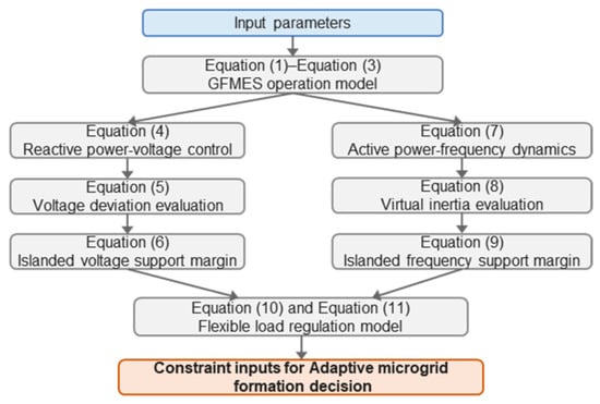
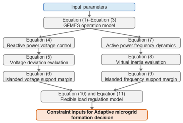
To clarify the logical relationship among the above models, Figure 1 presents the block diagram linking Equations (1)–(11), where the DG operation properties, voltage/frequency-forming and regulation capability margins, and flexible load regulation capability are connected as constraint inputs for the subsequent adaptive MF decision model.
Figure 1.
Block diagram of source/load capability models and their links to the adaptive MF model.
2.1. Model of DG’s Voltage/Frequency-Forming and Regulation Capabilities
To characterize the DG’s voltage/frequency-forming and regulation capabilities, GFMES is utilized as the main source for MF. Based on the virtual synchronous generator (VSG) control principle, a margin model for its voltage/frequency-forming and regulation capabilities is established to characterize the DG’s voltage/frequency-forming and regulation capabilities.
2.1.1. Model of DG’s Operation Properties
The forming and regulation capabilities of GFMES are based on their own energy and charge/discharge power limits. To this end, this subsection establishes the operation properties model of GFMES, including equality constraints on the state of charge (SOC), upper- and lower-bound constraints on energy storage charge and discharge power, and safety operating boundary constraints on energy storage capacity, as shown below:
where SOCb(t) and are the state of charge and the power of GFMES unit b at time instant t; and / are the rated capacity and the maximum/minimum state-of-charge values of GFMES unit b, respectively; and are the maximum charging and discharging power of GFMES unit b, respectively; B is the set of GFMES units; and ∆t is the length of a single time period of the MF.
2.1.2. Model of Voltage/Frequency-Forming and Regulation Capabilities
To characterize the DG’s voltage/frequency-forming and regulation capabilities, this subsection establishes a model for its voltage/frequency-forming and regulation capabilities based on the VSG control principle.
(1) Characterization of voltage-forming and regulation capabilities
To characterize the DG’s voltage/frequency-forming and regulation capabilities, a corresponding model is established based on the VSG control principle.
The VSG control of GFMES enables it to have voltage-forming and regulation capabilities by simulating the voltage regulation characteristics of synchronous generators through the reactive power–voltage control loop [22]. Its reactive power–voltage control equation is:
where Us is the virtual internal electromotive force of the GFMES, and U0 is the no-load electromotive force, and Kq is the reactive power–voltage droop coefficient, and Q0 is the reactive power reference value, and Q is the actual reactive power output of the GFMES.
Us = U0 − Kq(Q − Q0)
It should be noted that Equation (4) is not included as a constraint in the adaptive MF strategy model. Instead, this equation is used to calculate the voltage-forming and regulation capability margin of the GFMES. The calculated margin is then incorporated into the microgrid formation optimization model as a constraint.
The voltage-forming and regulation capabilities of GFMES depend on whether the voltage deviations of each node during islanded operation are within the allowable range [23]. Therefore, the voltage deviations of nodes within the island are used as the core indicator to characterize this capability, as shown below:
where αV is the total voltage deviation index for GFMES at all time instants, and Vi,t is the per-unit voltage value of node i within the island at time instant t, and Vi,N is the system voltage reference value, and T is the set of all time instants for adaptive microgrid formation.
Based on the above characterization of the voltage-forming and regulation capabilities of GFMES, considering the voltage deviation limit requirements under power disturbances during the stage of the microgrid’s islanded operation, this paper further establishes a margin model for its voltage-forming and regulation capabilities to assess the overall voltage deviation over the entire time horizon, expressed as:
where is the maximum allowable voltage deviation during the microgrid’s islanded operation.
(2) Characterization of frequency-forming and regulation capabilities
To characterize the frequency-forming and regulation capabilities of GFMES, a margin model is established based on the VSG control principle and the equivalent virtual inertia time constant of GFMES.
The VSG control of GFMES enables it to have frequency-forming and regulation capabilities by simulating the rotor motion equations of synchronous generators [24]. Its rotor motion equation is:
where J is the virtual moment of inertia; ω0 is the rated angular velocity; ωs is the virtual rotor angular velocity; P0 is the active power reference; P is the actual active power output of the GFMES; Kp is the active power–frequency droop coefficient; and Dp is the virtual damping coefficient.
It should be noted that Equation (7) is not included as a constraint in the adaptive MF strategy model. Instead, this equation is used to calculate the frequency regulation capability margin of the GFMES. The calculated margin is then incorporated into the microgrid formation optimization model as a constraint.
The frequency-forming and regulation capabilities of GFMES depend on whether its virtual inertia is sufficient to adapt to active power disturbances during islanded operation [25]. To evaluate the frequency-forming and regulation capabilities of GFMES during islanded operation, the virtual inertia time constant is adopted as the key metric [26]. It characterizes the ability of the energy storage system, under its current operating state, to mitigate frequency fluctuations, and is expressed as follows:
where Hb,t is the inertia time constant of GFMES unit b at time instant t, unit s; Qb(t) is the remaining capacity of the GFMES unit b at time instant t, unit kWh; is the dimensionless normalization coefficient for the rated capacity of the GFMES units, and the value is 1 in the simulation; S0 is the unit base power, unit MVA; and γmax is the maximum charge/discharge rate of the energy storage converter, dimensionless, and the value is 0.5.
Based on the above characterization of virtual inertia, a frequency-forming and regulation capability margin model is further developed to ensure that the GFMES can withstand power disturbances during islanded operation. In this model, the actual inertia provided by the GFMES must be greater than the minimum inertia required to limit the maximum rate of change of frequency, which is expressed as follows:
where fN is the rated system frequency, taking 50 Hz; ΔPmax is the maximum power variation caused by the system fault, taking 0.104 p.u.; is the maximum rate of change of frequency under the fault, taking 2.0 Hz/s; and Hloss is the system inertia loss after the fault, taking 1.25 s. The above main threshold parameters are selected according to Ref. [27].
It should be noted that Hloss represents the system inertia loss after the fault, caused by the disconnection or tripping of sources. A loss indicator Hloss indicates a more severe inertia deficiency and thus a higher requirement on GFMES frequency support capability.
2.2. Model of Flexible Load Regulation Capability
To fully exploit the regulation potential of flexible loads and ensure MF and its reliable islanded operation, it is necessary to characterize the regulation capability of flexible loads.
Distribution networks generally include three types of flexible loads: interruptible, curtailment, and shiftable loads. This paper characterizes the regulation capability of these three types of flexible loads, respectively, with the regulation models as follows:
where PLoad,i(t) is the forecasted load at node i at time instant t; ΔPLoad,int,i(t), ΔPLoad,cut,i(t) and ΔPLoad,sl,i(t) denote the adjustable active power of the interruptible load, curtailable load and shiftable load, respectively, at node i at time instant t; γi is the binary state variable of the flexible load; Ui,t is the interruption status variable of the interruptible load; αi is the curtailment coefficient of the curtailable load; and βi is the participation coefficient of the shiftable load.
∆PLoad,int,i(t) = γiUi,tPLoad,i(t)
0 ≤ ∆PLoad,cut,i(t) ≤ γiαiPLoad,i(t)
−γiβiPLoad,i(t) ≤ ∆PLoad,sl,i(t) ≤ γiβiPLoad,i(t)
2.3. Model of NBSA Limits
To avoid excessive NBSA, satisfy the distribution network’s requirements for the limits of NBSA, and ensure the feasibility of MF, this section proposes a constraint characterization method considering the limits on NBSA for both a single time period and adjacent time periods to characterize the limits on NBSA during the stage of MF.
(1) The limits of NBSA for a single time period
During the stage of MF, to limit NBSA on the distribution network within a single time period, the NBSA within a single time period shall not exceed the maximum allowable NBSA. The corresponding constraint is:
where Bk,t is the status of breaker k at time instant t, with 0 indicating open status and 1 closed; and is the maximum allowable NBSA in time period t.
(2) The limits of NBSA between adjacent time periods
During the stage of MF, to avoid excessive NBSA between adjacent time periods, the limits of NBSA between adjacent time periods are introduced, as shown below:
where is the maximum allowable NBSA of breaker k between adjacent time periods (taking a value of 0 or 1, where 0 indicates that the switch is not allowed to operate between adjacent time periods); and NB is the number of controllable breakers in the distribution network.
3. Adaptive MF Strategy
To analyze the impact of voltage/frequency-forming and regulation capabilities, flexible load regulation capability, and the limits of NBSA on MF and its islanded operation, making the MF method adaptive to power disturbances during the above stages, this paper integrates the voltage/frequency-forming and regulation capability model, flexible load regulation capability model, and NBSA constraint model established in Section 1 into the adaptive MF process. With the objective of maximizing the load restoration quantity over short-term and long-term scales, an adaptive MF decision model is established.
3.1. Objective Function
To reflect the load restoration effects at different time scales and to restore critical loads as much as possible, while embodying the goal of maximizing the load restoration quantity during the stage of MF and its islanded operation, load priority weights are introduced into the objective function to incorporate both short-term and long-term weighted load restoration quantities. The objective function is:
where L is the set of flexible loads; ci is the actual electricity consumption level of flexible load i; ωi and ωj are the load priority weights at node i, j; and μj is the binary state variable of the rigid load at node j.
3.2. Constraints
To establish a complete constraint system, this subsection incorporates DG’s forming and regulation capability, flexible load regulation capability, and NBSA constraints into the decision-model constraints, together with power flow constraints and island connectivity constraints during the stage of MF and its islanded operation, forming the constraint system of the adaptive MF decision model.
3.2.1. Power Flow Constraints
This section establishes the power flow constraints of the adaptive MF decision model, including islanded operation active power balance constraints, node voltage constraints, and branch current constraints, to ensure the power balance and safe operation of the island in each time period.
(1) Active Power Balance Constraints for Islanded Microgrid Operation
where , PDG,i(t), PLoss(t) are the charge/discharge power of energy storage unit i, the active power output of the i-th DG, and the network loss of the microgrid, respectively, at time instant t; and Is is the set of DG/load resources in the microgrid.
It should be noted that the network loss of the microgrid PLoss(t) and node voltages are calculated by solving the power flow using the MATPOWER toolbox during the constraint verification process.
(2) Node Voltage and Branch Current Constraints
To ensure the microgrid’s reliable islanded operation, the voltage and current of each node within the island shall satisfy the following constraints:
where vi, , and denote the voltage at node i and its upper and lower limits, respectively; N denotes the set of nodes in the distribution network; and lij and denote the squared current of the branch between nodes i and j and its maximum value, respectively.
3.2.2. Island Connectivity Constraints
To avoid invalid topologies such as isolated nodes or paths without actual power supply during the stage of MF, connectivity constraints during the MF process need to be considered, as shown below:
where Gt denotes the set of feasible microgrid topologies at time instant t, satisfying connectivity, radiality, and operational feasibility. In the proposed graph-theoretic solution procedure, gt ∈ Gt is implemented through the improved Kruskal search process rather than only treated as an abstract set constraint.
gt ∈ Gt
Mathematically, the radiality and connectivity of the formed microgrid can be defined by the tree constraints: (1) the number of energized branches equals the number of energized nodes minus the number of microgrids; (2) each load node has exactly one path to a GFMES node. Although these can be formulated using Mixed-Integer Linear Programming (MILP) with virtual flow constraints, the incorporation of dynamic NBSA limits, SOC time-coupling, and nonlinear voltage/frequency margins makes the exact MILP formulation highly complex (or intractable for large systems). Therefore, a graph-theoretic heuristic is employed.
Specifically, the topology construction follows the procedure of GFMES-rooted island initialization, candidate branch testing, cycle detection, constraint verification, and acceptance or rejection. A candidate branch is further tested only when it connects an unserved load node to an existing energized island or supports the feasible merging of two islanded subgraphs. This rule ensures that each restored load node has a valid supply path to at least one GFMES. Cycle detection is then used to reject branches that would create loops, thereby maintaining radiality. After that, the candidate topology is checked against power balance, SOC, voltage/frequency-forming and regulation capability margins, flexible load constraints, and NBSA limits. Therefore, under these rules, each accepted microgrid topology satisfies the connectivity, radiality, and operational feasibility requirements defined in the proposed model.
3.2.3. Summary of Constraints for the Adaptive MF Decision Model
Based on the characterization of DG’s forming and regulation capability, flexible load regulation capability, and NBSA constraints in Section 1, combined with the above power flow constraints and island connectivity constraints, the overall constraints of the adaptive MF decision model are as follows:
The complete optimization model is established from Equations (1)–(20). It is worth noting that this model integrates discrete decisions (breaker states, graph topology) with continuous physical constraints (power flow, SOC dynamics, voltage/frequency margins). To avoid the computational burden of formulating a full Mixed-Integer Nonlinear Programming (MINLP) problem, the next section elaborates on how the improved Kruskal algorithm is employed as a heuristic greedy approach to efficiently obtain a feasible and high-quality solution, where graph search and constraint verification are alternately performed.
4. Solution Algorithm
To efficiently solve the above adaptive MF decision model, this section employs an improved Kruskal algorithm [13]. The improved Kruskal algorithm is used to construct feasible radial islanded topologies under multiple operational constraints. Different from the classical Kruskal algorithm for a standard minimum spanning tree problem, the proposed algorithm embeds constraint checking into the branch-selection process. Each candidate branch is accepted only after radiality, connectivity, power balance, SOC, voltage/frequency-forming and regulation capability margins, flexible load regulation constraints, and NBSA limits are verified. In this way, the adaptive MF problem is transformed into a constrained subtree search problem, where graph search and constraint verification are alternately performed over multiple rolling time periods.
4.1. Graph Representation and Edge Weighting
The distribution network is modeled as an undirected connected graph G = (V,E). To clearly map the load attributes to the branches, the V nodes are categorized into three types: bus nodes, load nodes, and GFMES nodes. The system-side substation is defined as the root node (with a topological depth of 1). Correspondingly, the edges E represent the physical connections between these nodes (e.g., bus-to-bus branches, bus-to-load lines, and bus-to-GFMES lines).
To prioritize the restoration of critical loads and closer nodes, and to determine the search priority of candidate branches, a branch priority weight Wi is defined for edge i (connecting node u to node v) as follows:
where Si is the priority score of the load connected by branch i (3 for the first-level load, 2 for the second-level load, and 1 for the third-level load); LNi is the normalized per-unit value of the load, ranging from 0 to 1; and depth(νi) denotes the topological depth of node νi in the original radial topology of the active distribution network. The system-side power source is taken as the root node, whose depth is defined as 1. Along the power flow direction, the depth increases by 1 each time a downstream branch is passed. A larger depth value indicates that the node is farther from the system-side power source and closer to the end of the distribution network. λ1, λ2, and λ3 are the weighting coefficients of the corresponding terms, respectively. Here, λ1 > λ2 is used to reflect that load priority is given precedence over load size. In this paper, λ1 = 1, λ2 = 0.5, and λ3 = 0.5. Based on the branch priority weight, candidate branches are searched in descending order of Wi. A larger Wi indicates a higher search priority.
4.2. Algorithmic Implementation Procedure
The proposed improved Kruskal algorithm transforms the adaptive MF problem into a constrained subtree search problem, where graph search and constraint verification are alternately performed over multiple rolling time periods. The specific steps are as follows:
(1) Initialization and Parameter Input
Input the network topology, system parameters, GFMES states, breaker states, and forecasted outputs of PV, wind, storage, and loads for the current time period, and assign load priority weights to each node.
(2) Branch Expansion and Constraint Verification
Search the candidate branches sequentially based on the sorted priority weight. For each selected candidate branch that connects an unserved load node to an existing energized island, a trial addition is performed. According to the overall constraint system summarized in Equation (20) of Section 3.2.3, the algorithm then sequentially verifies the following constraints to ensure operational feasibility:
(a) Connectivity and Radiality (Equation (19)): Cycle detection is executed to ensure that adding the branch does not create a loop, thereby maintaining the radial structure.
(b) AC Power Flow and Power Balance (Equations (16)–(18)): The MATPOWER toolbox is invoked to solve the AC power flow for the candidate island. The actual network loss and node voltages are calculated to strictly verify the active power balance of Equation (16), node voltage limits of Equation (17), and branch current limits of Equation (18).
(c) GFMES Capability Margins (Equations (1)–(3), (6), (9)): The state of charge (SOC) limits and power bounds are checked using Equations (1)–(3). The voltage and frequency-forming capability margins are evaluated via Equations (6) and (9) to ensure reliable islanded operation.
(d) Flexible Load Constraints (Equations (10)–(12)): The regulation limits of interruptible, curtailable, and shiftable loads are verified to ensure the load adjustment remains within the allowable range.
(e) NBSA Limits (Equations (13)–(14)): The switching actions are evaluated against both the single-period limit of Equation (13) and the adjacent-period state change limit of Equation (14).
If all constraints are satisfied, the candidate branch and the corresponding node are included in the corresponding islanded subgraph; otherwise, the algorithm backtracks and tests the next candidate node or branch. This process continues until no feasible candidate branch remains, all restorable loads have been included, or the current island reaches the power balance, SOC, voltage/frequency capability, or NBSA boundary.
The backtracking mechanism is implemented through trial addition and rejection. Specifically, when a candidate branch is tested, the topology and operational states are temporarily updated. If any constraint is violated, the branch is removed, and all related states are restored to the values before the trial addition.
(3) Island Merging and Tie-Breaking
If some microgrids have reached the power balance limit and cannot accept more loads, but there remain load nodes not included in any microgrid, candidate inter-island branches are tested in descending order of branch priority weight to merge two microgrids. Constraint verification is then performed on the merged MF scheme. If all constraints are satisfied, the merge is accepted; otherwise, the original microgrid boundaries are maintained, and the next candidate inter-island branch is tested.
For equivalent candidate branches with the same branch priority weight, the tie-breaking rule is applied sequentially. The branch connected to the higher-priority load is selected first. If the load priority is still the same, the branch with the larger load restoration increment is selected. If the tie remains, the branch with the larger remaining voltage/frequency-forming and regulation capability margin is selected. Finally, the branch with the smaller branch index is selected to ensure deterministic implementation.
(4) ESS Power Calculation and SOC Update
After the initial topology is determined, the required charge/discharge power for each GFMES is calculated based on the total load and renewable generation within its island. The actual power is restricted by the maximum power limits and the SOC bounds. Subsequently, the SOC for each GFMES is updated for the current time period, and the available DG capacity is revised for the subsequent final adjustment.
Refine the formed microgrid topology. After completing the microgrid searches in Steps (2) and (3), if there remain nodes without connected loads, remove them from the microgrid to ensure that all retained nodes belong to successfully formed microgrids, thereby obtaining the MF result for the current time period.
(5) Topology Refinement
Refine the formed microgrid topology. Based on the updated SOC and DG capacity, a final adjustment is performed. If there remain nodes without connected loads, remove them from the microgrid to ensure that all retained nodes belong to successfully formed microgrids, thereby obtaining the final MF result for the current time period.
(6) State Update and Multi-Period Rolling
Output the adaptive MF result for the current time period. Update the microgrid’s operational state (including energy storage’s SOC, flexible load, network topology, and breaker status). Take the updated states as the initial states for the next time period while inputting the DG output and load data for the next time period. Repeat steps (1)–(5) until the MF for all time periods is completed.
4.3. Pseudocode of the Proposed Algorithm
To eliminate any ambiguity in the programmatic implementation and to enhance the reproducibility of this study, the complete procedure of the proposed improved Kruskal algorithm is summarized in Algorithm 1.
| Algorithm 1. Improved Kruskal Algorithm for Adaptive Microgrid Formation |
| ------------------------------------------------------------------------- Input: Network topology G(V,E), faulted lines, load priority weights, DG/GFMES parameters (SOC_0, P_max, E^N), constraint limits, and total time horizon T. Output: Per-period microgrid formation schemes g_t, breaker states B_t, and load restoration quantities. ------------------------------------------------------------------------- 1: Initialize system states: SOC(1) ← SOC_0, B(1) ← B_0. 2: for time period t = 1 to T do 3: Set available GFMES nodes as the initial roots of candidate islands. 4: Calculate branch priority weights W_i for all candidate edges using Equation (21). 5: Sort the candidate branches in descending order of W_i. 6: 7: // Phase 1: Branch Expansion and Initial Topology Formation 8: for each candidate branch e in the sorted list do 9: if e connects an unserved load node to an energized island then 10: Perform trial addition for branch e. 11: Invoke MATPOWER to solve the AC power flow for the candidate island. 12: Sequentially check: 13: -Connectivity and Radiality (Equation (19)) 14: -Power Balance (Equation (16)), Voltage (Equation (17)), Current (Equation (18)) 15: -SOC bounds (Equation (3)) and V/f Margins (Equations (6) and (9)) 16: -Flexible Load limits (Equations (10)–(12)) 17: -Single and Adjacent-period NBSA limits (Equations (13) and (14)) 18: if all constraints are satisfied then 19: Accept branch e; Update topology. 20: else 21: Reject branch e; Trigger backtracking to revert states. 22: end if 23: end if 24: end for 25: 26: // Phase 2: Island Merging and Tie-Breaking 27: while unserved load nodes remain AND number of islands > 1 do 28: Select the inter-island branch e_merge with the maximum W_i. 29: Perform trial addition for e_merge and run MATPOWER. 30: if all constraints are satisfied then 31: Accept merge and update topology. 32: else 33: Reject merge and maintain original boundaries. 34: end if 35: end while 36: 37: // Phase 3: ESS Power Calculation and SOC Update 38: for each formed island in the current period do 39: Calculate the required ESS power (P_ess) based on island load and generation. 40: Constrain P_ess by power limits and SOC bounds (Equations (1)–(3)). 41: Update SOC(t) for the current time period. 42: end for 43: 44: // Phase 4: Final Topology Refinement and State Update 45: Perform final topology adjustment using the updated SOC(t). 46: Remove isolated nodes without supply paths to any GFMES. 47: Record MF scheme g_t, load restoration, and NBSA count for period t. 48: Update breaker states B(t + 1) for the next period. 49: end for 50: Return g_t, B_t, and load restoration results. ------------------------------------------------------------------------- |
4.4. Optimality and Heuristic Nature
It should be noted that the proposed improved Kruskal algorithm is a heuristic greedy algorithm. Although the objective function in Equation (15) is formulated as a maximization problem, the proposed algorithm is not claimed to guarantee the global optimum of the full MF problem.
The classical Kruskal algorithm guarantees optimality only for standard minimum spanning tree problems without additional time-coupled physical and operational constraints. In contrast, the proposed adaptive MF model includes SOC constraints, voltage/frequency-forming and regulation capability margins, NBSA limits, power balance constraints, flexible load regulation constraints, and islanded operation constraints. Moreover, the actual network losses and node voltages are calculated by the nonlinear AC power flow (via MATPOWER). These physical and temporal constraints break the standard optimality conditions (matroid structure) of the classical Kruskal algorithm, making the formulation of an exact MINLP model highly complex or intractable for standard commercial solvers.
Therefore, the proposed algorithm aims to obtain a feasible and high-quality solution efficiently under post-fault restoration time requirements, rather than to provide a global optimality guarantee.
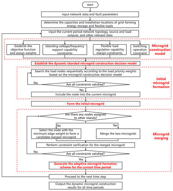
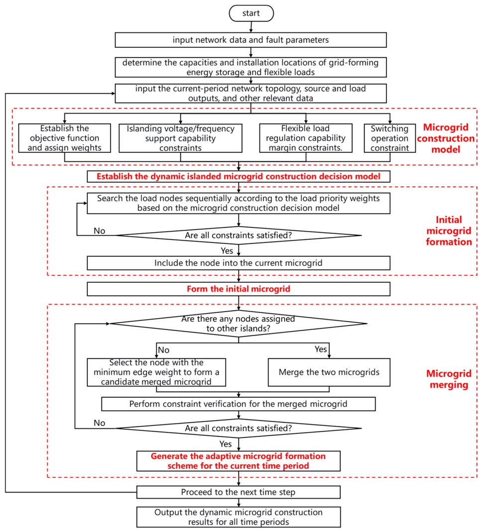
Finally, to provide a clearer and more intuitive overview of the proposed solution, the complete execution procedure of the improved Kruskal algorithm is visualized in the flowchart shown in Figure 2. This flowchart systematically illustrates the entire constrained subtree search process, encompassing the initial input of system parameters, the generation of initial islands based on GFMES nodes, the iterative branch expansion (with trial addition and backtracking), the island merging operations, and the multi-period rolling state updates. It explicitly reflects how the graph search and sequential constraint verification (from MATPOWER power flow to NBSA limits) are alternately performed to guarantee the feasibility and reliability of the final microgrid formation scheme.
Figure 2.
Flowchart of the proposed adaptive MF method.
5. Simulation
5.1. Simulation Setup
To verify the effectiveness of the proposed method, case models are established on the MATLAB/Simulink (R2023b) simulation platform and the improved IEEE 33-bus distribution network. The relevant simulation parameters are set as follows.
(1) Simulation model parameter settings: To simulate power disturbances during the stage of the microgrid’s islanded operation, this paper takes the microgrid formed in the 16th time period after the fault as an example and builds a corresponding simulation model with GFMES as the main source. The same active power disturbance (30 kW) and reactive power disturbance (30 kVar) are applied. The characteristic parameters of the DGs are given in Table 1.
Table 1.
DG location and capacity.
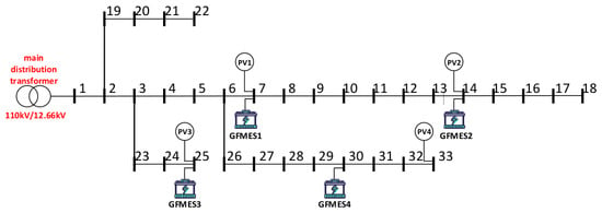
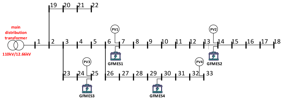
(2) Distribution network parameter settings: The topology of the distribution network is shown in Figure 3. The load priority weights of each node are shown in Table 2, and the nodes with various types of flexible loads are shown in Table 3. The initial breaker status of all lines in the system is set to closed. To simulate the distribution network fault scenario, line 1-2 is set to fail at 8:00, causing loss of power supply in the downstream area of this line. The outage duration is 4 h, and the MF time scale is 15 min.
Figure 3.
Schematic diagram of the topological structure of the modified IEEE 33-bus distribution network. GFMES: grid-forming energy storage.
Table 2.
Load priority weight settings.
Table 3.
Flexible-load node settings.
To improve reproducibility and transparency, the key parameters, limits, and data sources used in the simulation are summarized in Table 4. These parameters include the system parameters, VSG control parameters, droop coefficients, voltage and frequency limits, the rate of change of frequency (RoCoF) limits, NBSA limits, and the time-series inputs. The parameters are either taken from the standard IEEE 33-bus system, set according to relevant grid codes and literature, or selected based on the operating requirements of the modified test system. Specifically, the proposed method maintains sufficient margins for voltage, frequency, RoCoF, SOC, and switching actions, which indirectly indicates its robustness to parameter variations. A more comprehensive sensitivity analysis will be considered in future work.
Table 4.
Key simulation parameters, limits, and data sources.
To analyze the impacts of the DG’s voltage/frequency-forming and regulation capabilities and the NBSA constraint on the load restoration quantity and the NBSA, and to evaluate the effectiveness of the proposed strategy, four schemes are defined for comparative analysis.
(1) Method 1: Conventional Microgrid Formation (CMF). This method utilizes GFMES and relies solely on static power balance, without considering the voltage/frequency-forming capability of the sources or the NBSA limits.
(2) Method 2: MF with the NBSA constraint. This method utilizes GFMES and incorporates the NBSA limits into the constraints. However, the voltage/frequency-forming and regulation capability margins are not considered.
(3) Method 3: MF with the voltage/frequency-forming and regulation capability constraint. This method utilizes GFMES and incorporates the voltage/frequency-forming and regulation capability margins into the constraints. However, the NBSA limits are not considered.
(4) Method 4: Adaptive Microgrid Formation Strategy (AMFS). This method utilizes GFMES. It incorporates the voltage/frequency-forming and regulation capability margins and the NBSA limits into the constraints, ensuring both system stability and operational feasibility during the MF process.
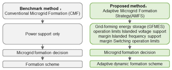
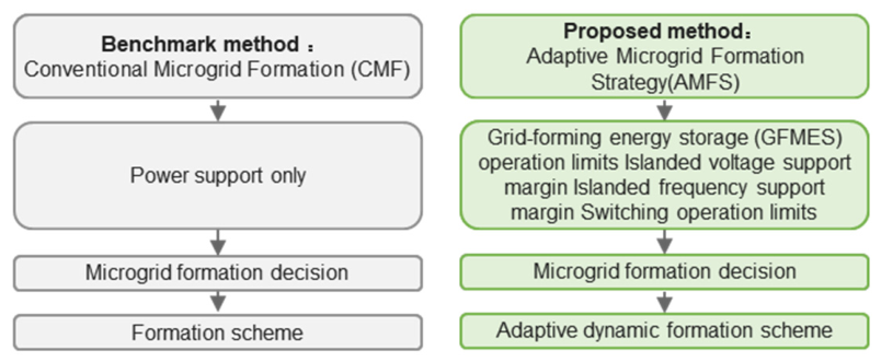
The frameworks of these two methods are compared in Figure 4:
Figure 4.
Framework comparison between methods CMF and AMFS.
5.2. Simulation Result Analysis
5.2.1. Analysis of MF Results
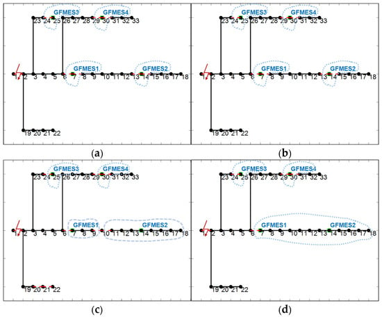
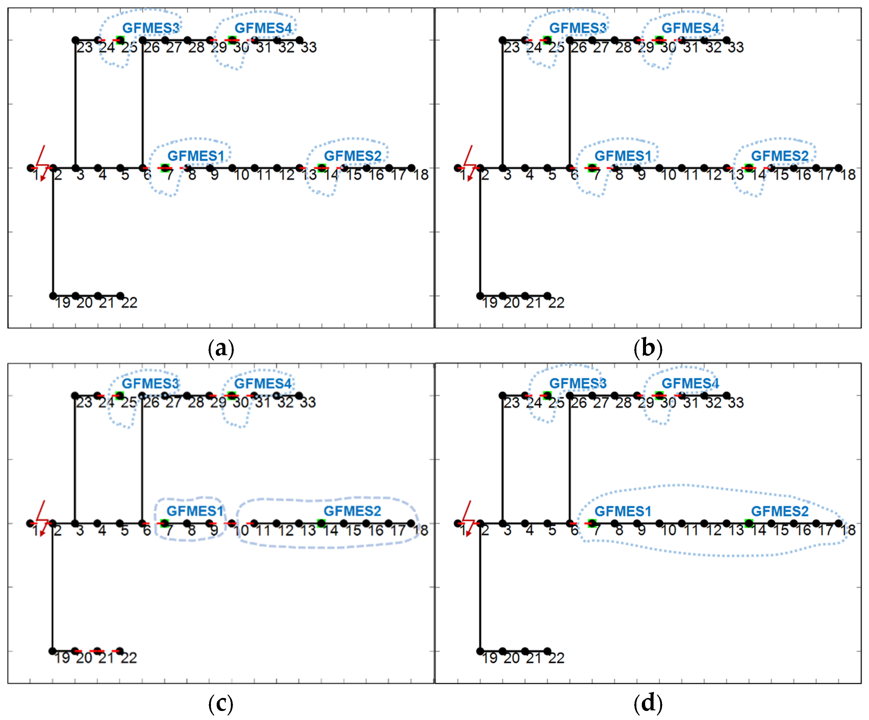
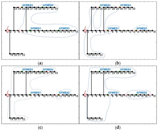
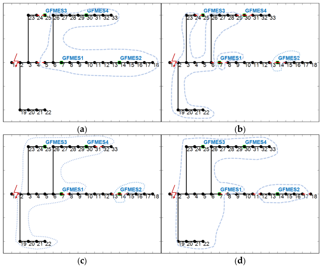
To verify the effectiveness of the proposed method in achieving microgrid formation and topological expansion, this subsection compares the topological evolution results under the four methods. Figure 5 shows the MF results in the first time period after the fault, and Figure 6 shows the results in the 16th time period. In the figures, Method 1 denotes traditional MF without either constraint, Method 2 denotes MF with the limits of NBSA only, Method 3 denotes MF with the voltage/frequency-forming and regulation capability constraint only, and Method 4 denotes the proposed method with both constraints.
Figure 5.
MF results of different methods in the first time period under (a) Method 1, (b) Method 2, (c) Method 3, and (d) Method 4. The dashed circles indicate the open status of the line switches, the green dots indicate the nodes connected with GFMES, and the numbers denote the bus indices. GFMES: grid-forming energy storage.
Figure 6.
MF results of different methods in the 16th time period under (a) Method 1, (b) Method 2, (c) Method 3, and (d) Method 4. The dashed circles indicate the open status of the line switches, the green dots indicate the nodes connected with GFMES, and the numbers denote the bus indices. GFMES: grid-forming energy storage.
It can be observed from Figure 5a,b that in the first time period, Methods 1 and 2, which do not consider the voltage/frequency-forming and regulation capability constraint, fail to adapt to initial power disturbances, resulting in four isolated microgrids that cover fewer restored loads. In contrast, as shown in Figure 5c,d, Methods 3 and 4, which consider the voltage/frequency-forming and regulation capability constraint, successfully construct three larger-scale initial islands and cover more loads by leveraging the forming capability of GFMES. This indicates that the voltage/frequency-forming and regulation capability constraint plays a key role in determining the load restoration quantity and the scale of microgrid formation during the MF stage.
Furthermore, as shown in Figure 6c,d, in the 16th time period, Methods 3 and 4 safely merge adjacent microgrids to further construct two larger-scale islands, thereby incorporating broader load areas. The fundamental reason for this topological evolution is that these two methods evaluate the GFMES’s voltage/frequency-forming and regulation capability margins. This evaluation guarantees the necessary stability margins for microgrid merging and continuous load restoration while satisfying the limits of NBSA (for Method 4) or without considering the limits of NBSA (for Method 3). In contrast, as shown in Figure 6a,b, although Methods 1 and 2 also evolve into two islands, they cover fewer nodes compared to Methods 3 and 4. They fail to incorporate more boundary loads, and their overall restoration scope remains restricted due to the lack of adaptive regulation capability for expansion. These results further confirm that the voltage/frequency-forming and regulation capability constraint is the primary factor affecting the load restoration quantity and the microgrid formation scope, whereas the limits of NBSA mainly affect the switching actions.
5.2.2. Analysis of Islanded Microgrid Operation Results
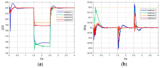
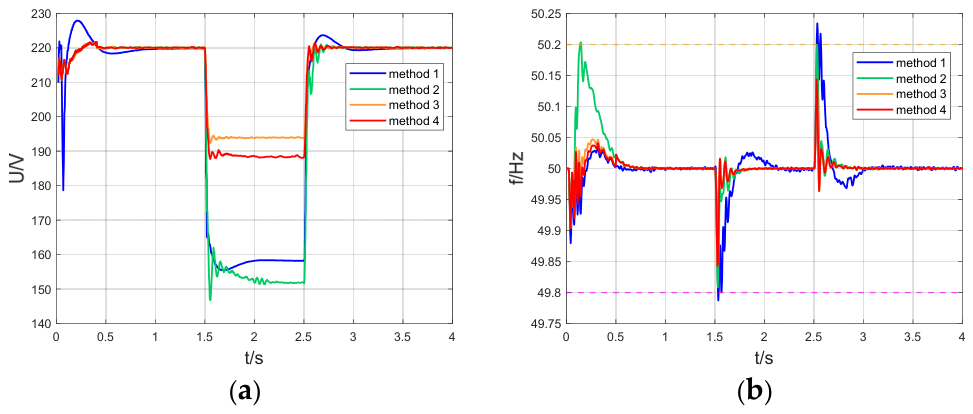
Figure 7a,b show the voltage and frequency response curves of the four methods during the microgrid islanded operation stage. Comparing Method 2 and Method 4, both consider the limits of NBSA, but Method 4 additionally considers the voltage/frequency-forming and regulation capability constraint. As a result, Method 4 significantly outperforms Method 2 in terms of voltage sag depth and maximum frequency deviation. Similarly, comparing Method 1 and Method 3, neither considers the limits of NBSA, but Method 3 considers the voltage/frequency-forming and regulation capability constraint. Method 3 exhibits noticeably better voltage and frequency responses than Method 1.
Figure 7.
Voltage/frequency response curves of different methods under (a) voltage response curves, and (b) frequency response curves. The yellow dotted lines indicate the upper frequency limit, and the pink dotted lines indicate the lower frequency limit.
These comparisons indicate that the voltage/frequency-forming and regulation capability constraint is the primary factor affecting the voltage and frequency response characteristics of the microgrid. The fundamental reason is that methods considering this constraint (Methods 3 and 4) ensure the formed microgrid can adapt to power disturbances during islanding, whereas methods neglecting this constraint (Methods 1 and 2) solely consider the load-serving capability of DGs and fail to adapt to power disturbances. Consequently, incorporating the voltage/frequency-forming and regulation capability constraint successfully empowers the formed microgrid to adapt to power fluctuations, thereby guaranteeing its reliable islanded operation.
The detailed quantitative comparison of the voltage/frequency-forming and regulation capabilities is provided in Table 5. To isolate the effect of the voltage/frequency-forming and regulation capability constraint, a controlled-variable comparison is conducted.
Table 5.
Comparison of voltage/frequency-forming and regulation capabilities.
First, comparing Method 2 and Method 4, both consider the limits of NBSA, but Method 4 additionally considers the voltage/frequency-forming and regulation capability constraint. As shown in Table 5, Method 4 achieves smaller voltage sag depth, smaller maximum frequency deviation, lower maximum frequency change rate, and shorter recovery times than Method 2. This indicates that the voltage/frequency-forming and regulation capability constraint significantly improves the voltage and frequency responses.
Similarly, comparing Method 1 and Method 3, neither considers the limits of NBSA, but Method 3 considers the voltage/frequency-forming and regulation capability constraint. Method 3 also exhibits better voltage and frequency performance than Method 1.
This ablation study consistently shows that the voltage/frequency-forming and regulation capability constraint is the primary factor affecting the voltage and frequency response characteristics during islanded operation. The fundamental reason is that Methods 3 and 4 consider the DG’s voltage/frequency-forming and regulation capabilities, enabling the microgrid to adapt to power disturbances during islanded operation, whereas Methods 1 and 2 only consider the DG’s load-serving capabilities, resulting in their inability to adapt to power disturbances during islanded operation. The above results further verify that the voltage/frequency-forming and regulation capability constraint is the key factor enabling the formed microgrid to adapt to power disturbances during islanded operation, thereby ensuring the microgrid’s reliable islanded operation.
5.2.3. Comprehensive Analysis of MF and Islanded Operation Results
Table 6 presents the comprehensive comparison results of the four methods during the MF and islanded operation stages. To isolate the contribution of each constraint, an ablation study is conducted.
Table 6.
Comparison of MF and its islanded operation effects under different methods.
(1) In terms of MF and its islanded operation
Overall, Methods 3 and 4, which consider the voltage/frequency-forming and regulation capability constraint, achieve significantly higher short-term and long-term weighted load restoration quantities and lower average voltage deviations than Methods 1 and 2, which do not consider this constraint.
During the stage of MF, comparing Method 2 and Method 4, both consider the limits of NBSA, but Method 4 additionally considers the voltage/frequency-forming and regulation capability constraint. As shown in Table 6, Method 4 achieves significantly higher short-term and long-term weighted load restoration quantities and a lower average voltage deviation than Method 2. The fundamental reason is that Method 2 neglects the DG’s islanded voltage/frequency-forming and regulation capabilities, resulting in weak voltage/frequency-forming and regulation capabilities of the formed microgrid, which leads to MF failure and insufficient load restoration. In contrast, Method 4 takes these capabilities into account, ensuring that the microgrid possesses adequate islanded voltage/frequency-forming and regulation capabilities, thereby guaranteeing successful MF and improving the load restoration quantity. Similarly, comparing Method 1 and Method 3, neither considers the limits of NBSA, but Method 3 considers the voltage/frequency-forming and regulation capability constraint. Method 3 also achieves significantly higher load restoration quantities and a lower average voltage deviation than Method 1. The same reason applies: Method 1 neglects the voltage/frequency-forming and regulation capabilities, while Method 3 considers them, thus ensuring successful MF and a larger load restoration quantity. These controlled comparisons consistently show that the voltage/frequency-forming and regulation capability constraint is the primary factor affecting the load restoration quantity and voltage performance during the MF stage.
During the stage of the microgrid’s islanded operation, the same controlled-variable logic applies. Methods 3 and 4, which consider the voltage/frequency-forming and regulation capability constraint, enable the formed microgrids to adapt to power disturbances, thereby maintaining a larger restoration scope and lower voltage deviation. In contrast, Methods 1 and 2 neglect this capability, making the formed microgrids unable to adapt to power disturbances, which may lead to load shedding and a restricted restoration scope. These results further confirm that considering the DG’s voltage/frequency-forming and regulation capabilities enables the microgrid to adapt to power disturbances during islanded operation.
(2) In terms of NBSA
A controlled-variable comparison is also conducted for the limits of NBSA. Comparing Method 1 and Method 2, both neglect the voltage/frequency-forming and regulation capability constraint, but Method 2 considers the limits of NBSA. As shown in Table 6, the NBSA of Method 2 is significantly lower than that of Method 1, while the load restoration quantities and average voltage deviation change only slightly. Similarly, comparing Method 3 and Method 4, both consider the voltage/frequency-forming and regulation capability constraint, but Method 4 considers the limits of NBSA. The NBSA of Method 4 is significantly lower than that of Method 3, and the load restoration quantities further increase while the average voltage deviation further decreases. These results clearly show that the limits of NBSA mainly affect the number of switching actions, and incorporating them can also guide the algorithm toward a more feasible and higher-quality topology.
The fundamental reason is that Methods 1 and 3 neglect the limits of NBSA, causing excessive switching actions and failing to satisfy the distribution network’s requirements, which may render the MF infeasible. In contrast, Methods 2 and 4 establish the NBSA limits model, avoiding excessive switching actions and satisfying the distribution network’s requirements, thus ensuring the feasibility of MF. In particular, Method 3 achieves a high load restoration quantity but incurs a relatively large NBSA, which may exceed the allowable limit. Method 4, by considering both constraints, reduces the NBSA while achieving the highest load restoration quantity and the lowest average voltage deviation, demonstrating that the proposed method balances restoration performance and operational feasibility.
In summary, the above controlled comparisons consistently show that the voltage/frequency-forming and regulation capability constraint is the primary factor affecting the load restoration quantity and voltage performance, and that considering the DG’s voltage/frequency-forming and regulation capabilities enables the microgrid to adapt to power disturbances during islanded operation. Meanwhile, the limits of NBSA mainly affect the number of switching actions. The proposed Method 4 considers both constraints simultaneously and achieves the best overall performance.
6. Conclusions
To address the existing problems of insufficient load restoration quantity and excessive NBSA, this paper proposes an adaptive MF strategy considering the DG’s voltage/frequency-forming and regulation capabilities and the NBSA limits. Through analysis and validation, the following conclusions are drawn:
(1) The proposed method can maximize the load restoration quantity compared with traditional methods. The proposed method considers the DG’s voltage/frequency-forming and regulation capabilities. During the stage of MF, it provides voltage/frequency-forming and regulation capabilities to ensure successful formation. During the stage of the microgrid’s islanded operation, it ensures that the microgrid can adapt to power disturbances, thereby significantly maximizing the load restoration quantity.
(2) The proposed method can avoid excessive NBSA compared with traditional methods. The proposed method considers the limits of NBSA. During the stage of MF, it introduces the limits of NBSA to avoid excessive NBSA, satisfies the distribution network’s requirements for the limits of NBSA, and thus ensures the feasibility of MF.
Future work will include a comprehensive sensitivity analysis with respect to the disturbance magnitude, initial SOC, and NBSA limit to further validate the robustness of the proposed method under a wider range of operating conditions.
Supplementary Materials
The following supporting information can be downloaded at https://www.mdpi.com/article/10.3390/en19215192/s1, Figure S1: Daily load demand profile of the IEEE 33-bus system; Figure S2: Daily PV generation profile of the IEEE 33-bus system; Table S1: Branch impedance data of the IEEE 33-bus system; Table S2: Node injection power data of the IEEE 33-bus system; File S1: Original IEEE 33-bus benchmark data (case33bw.m); File S2: Time-series input profiles for loads and PV (IEEE33_Data_Export.xlsx).
Author Contributions
Conceptualization, R.C.; methodology, R.C. and F.X.; validation, R.C.; formal analysis, Y.C.; investigation, Y.Z.; resources, X.Q. and Y.H.; writing—original draft preparation, R.C.; writing—review and editing, F.X.; visualization, F.X.; supervision, F.X.; project administration, F.X. All authors have read and agreed to the published version of the manuscript.
Funding
This research is supported by the [Smart Grid-National Science and Technology Major Project] under grant number [Proj. #2025ZD0804500; Task #2025ZD0804502]. The APC is supported by the [Smart Grid-National Science and Technology Major Project] under grant number [Proj. #2025ZD0804500; Task #2025ZD0804502].
Data Availability Statement
This study is based on the publicly available IEEE 33-bus test system and simulation data. The original IEEE 33-bus benchmark data (branch impedance and injection power) and the time-series input profiles (load demand and PV generation) used in this study are provided in Tables S1 and S2 and Figures S1 and S2 of the Supplementary Materials and in the separate accompanying Excel files (packaged as a ZIP archive). All modifications to the test system, including the GFMES connection nodes and capacities (Table 1), load priority weights (Table 2), flexible-load node settings (Table 3), and key simulation parameters and limits (Table 4), are fully provided in the article. No confidential data are used. With the article and the Supplementary Materials taken together, all necessary parameters and input data are disclosed to reproduce the case study.
Conflicts of Interest
Authors Xuebo Qiao and Yuting Huang were employed by the company National Institute of Guangdong Advanced Energy Storage Co., Ltd. The remaining authors declare that the research was conducted in the absence of any commercial or financial relationships that could be construed as a potential conflict of interest. The authors declare that this study received funding from the Smart Grid-National Science and Technology Major Project. The funder was not involved in the study design, collection, analysis, interpretation of data, the writing of this article or the decision to submit it for publication.
Abbreviations
The following abbreviations are used in this manuscript:
| DG | distributed generation |
| GFMES | grid-forming energy storage |
| MF | microgrid formation |
| RoCoF | rate of change of frequency |
| MINLP | mixed-integer nonlinear programming |
| CMF | conventional microgrid formation |
| NBSA | number of breaker switching actions |
| VSG | virtual synchronous generator |
| SOC | state of charge |
| MILP | mixed-integer linear programming |
| AMFS | adaptive microgrid formation strategy |
Nomenclature
Symbol
| SOCb(t) | the state of charge of GFMES b at time instant t |
| the rated capacity of GFMES b | |
| the minimum SOC of GFMES b | |
| the maximum discharging power of GFMES b | |
| Us | the virtual internal potential of the GFMES |
| Kq | the reactive power–voltage droop coefficient |
| Q | the actual reactive power output of the GFMES. |
| Vi,t | the per-unit voltage of node i within the island at time instant t |
| T | the set of all time instants for adaptive microgrid formation |
| J | the virtual moment of inertia |
| ωs | the virtual rotor angular velocity |
| P | the actual active power output of GFMES |
| Dp | the virtual damping coefficient |
| Qb(t) | the remaining capacity of the GFMES unit b at time instant t |
| S0 | the unit base power |
| fN | the rated system frequency |
| the maximum rate of change of frequency under the fault | |
| ∆PLoad,int,i(t) | the adjustable active power of the interruptible load at node i at time instant t |
| Ui,t | the interruption state variable of the interruptible load at node i at time instant t |
| ∆PLoad,cut,i(t) | the adjustable active power of the curtailable load at node i at time instant t |
| ∆PLoad,sl,i(t) | the adjustable active power of the shiftable load at node i at time instant t |
| Bk,t | the status of breaker k at time instant t |
| the maximum allowable NBSA in time period t | |
| NB | the number of controllable breakers in the distribution network |
| ci | the actual electricity consumption level of flexible load i |
| μj | The binary state variable of the rigid load at node j |
| PLoss(t) | the network loss of the microgrid |
| vi | the voltage of node i |
| the minimum voltage limit of node i | |
| lij | the squared current of branch (i,j) |
| gt | the topology of the microgrid at time t |
| B | the set of GFMESs |
| LNi | the normalized per-unit value of the load, ranging from 0 to 1 |
| λ1,λ2,λ3 | the weighting coefficients of the load |
| the power of GFMES b at time instant t | |
| the maximum SOC of GFMES b | |
| the maximum charging power of GFMES b | |
| ∆t | the length of a single time period of the MF |
| U0 | the no-load electromotive force |
| Q0 | the reactive power reference value |
| αV | the total voltage deviation index for GFMES at all time instants |
| the system voltage reference value | |
| the maximum allowable voltage deviation of during the microgrid’s islanded operation | |
| ω0 | the rated angular velocity |
| P0 | the active power reference |
| Kp | the active power-frequency droop coefficient |
| Hb,t | the inertia time constant of GFMES unit b at time instant t |
| the dimensionless normalization coefficient for the rated capacity of the GFMES units | |
| γmax | the maximum charge/discharge rate of the energy storage converter |
| ΔPmax | the maximum power variation caused by the system fault |
| Hloss | the system inertia loss after the fault |
| γi | the binary state variable of the flexible load |
| PLoad,i(t) | the forecasted load at node i at time instant t |
| αi | the curtailment coefficient of the curtailable load |
| βi | the participation coefficient of the shiftable load |
| Bk,t−1 | the status of breaker k at time instant t − 1 |
| the maximum allowable NBSA of breaker k between adjacent time periods | |
| L | the set of flexible loads |
| ωi | the load priority weight of node i |
| PDG,i(t) | the active power output of the i-th DG at time t |
| Is | the set of DG/load resources in the microgrid |
| the maximum voltage limit of node i | |
| N | the set of nodes in the distribution network |
| the maximum squared current of branch (i,j) | |
| Gt | the set of topologies that satisfy the connectivity constraints |
| Si | the priority score of the load connected by branch i |
| depth(νi) | the topological depth of node νi in the original radial topology of the active distribution network |
| B | the set of GFMES units |
References
- Vijayan, V.; Arzani, A.; Mahajan, S.M. Network Reconfiguration in electric power distribution networks: A Review. IEEE Trans. Ind. Appl. 2026, 62, 5149–5159. [Google Scholar] [CrossRef] [Scilit]
- Shen, F.; Wu, Q.; Xue, Y. Review of service restoration for distribution networks. J. Mod. Power Syst. Clean Energy 2020, 8, 1–14. [Google Scholar] [CrossRef] [Scilit]
- Igder, M.A.; Liang, X.; Mitolo, M. Service restoration through microgrid formation in distribution networks: A Review. IEEE Access 2022, 10, 46618–46632. [Google Scholar] [CrossRef] [Scilit]
- Alobaidi, A.H.; Fazlhashemi, S.S.; Khodayar, M.; Wang, J.; Khodayar, M.E. Distribution service restoration with renewable energy sources: A Review. IEEE Trans. Sustain. Energy 2023, 14, 1151–1168. [Google Scholar] [CrossRef] [Scilit]
- Cao, H.; Gao, C.; Chen, P.; He, X.; Dong, Z.; Lin, L. Distribution network dynamic reconfiguration based on improved fuzzy C-Means clustering with time series analysis. IEEJ Trans. Electr. Electron. Eng. 2022, 17, 174–182. [Google Scholar] [CrossRef] [Scilit]
- Tian, J.; Li, A.; Gao, F.; Zhao, F.; Geng, F. Island partition of active distribution network with photovoltaic generation and time-varying loads. Acta Energiae Solaris Sin. 2021, 42, 125–131. [Google Scholar]
- Sun, W.; Liu, W.; Zhang, J. Coordinated optimization of dynamic reconfiguration and mobile energy storage in distribution networks under high penetration of renewable energy. Autom. Electr. Power Syst. 2021, 45, 80–90. [Google Scholar]
- Fathabadi, H. Power Distribution network reconfiguration for power loss minimization using novel dynamic fuzzy C-Means (dFCM) clustering based ANN approach. Int. J. Electr. Power Energy Syst. 2016, 78, 96–107. [Google Scholar] [CrossRef] [Scilit]
- Zhou, G.; Wu, Y.; Yu, T.; Pan, Z.; Liu, Q.; Chen, Z.; Zhao, R.; Li, H. An efficient dynamic reconfiguration for distribution networks via learning-assisted decision-oriented period division. Int. J. Electr. Power Energy Syst. 2025, 173, 111406. [Google Scholar] [CrossRef] [Scilit]
- Pan, J.S.; Wang, H.J.; Nguyen, T.T.; Zou, F.-M.; Chu, S.-C. Dynamic reconfiguration of distribution network based on dynamic optimal period division and multi-group flight slime mould algorithm. Electr. Power Syst. Res. 2022, 208, 107925. [Google Scholar] [CrossRef] [Scilit]
- Ji, X.; Zhang, X.; Zhang, Y.; Yin, Z.; Yang, M.; Han, X. Three-Phase symmetric distribution network fast dynamic reconfiguration based on timing-constrained hierarchical clustering algorithm. Symmetry 2021, 13, 1479. [Google Scholar] [CrossRef] [Scilit]
- Chen, Q.; Wang, W.; Wang, H.; Wu, J.; Li, X.; Lan, J. A social beetle swarm algorithm based on grey target decision-making for a multiobjective distribution network reconfiguration considering partition of time intervals. IEEE Access 2020, 8, 204987–205013. [Google Scholar] [CrossRef] [Scilit]
- Yi, X.; Lu, Y. Islanding Algorithm of distribution networks with distributed generators. Power Syst. Technol. 2006, 30, 50–54. [Google Scholar]
- Sahu, A.; Utkarsh, K.; Ding, F. A fast and scalable genetic algorithm-based approach for planning of microgrids in distribution networks. In Proceedings of the 2022 IEEE Power & Energy Society General Meeting (PESGM), Denver, CO, USA, 17–21 July 2022; pp. 1–5. [Google Scholar]
- Liu, M.; Wu, J.; Zhang, Q.; Zheng, H. Fault recovery of distribution network with distributed generation based on pigeon-inspired optimization algorithm. Electronics 2024, 13, 886. [Google Scholar] [CrossRef] [Scilit]
- Osama, R.A.; Zobaa, A.F.; Abdelaziz, A.Y. A planning framework for optimal partitioning of distribution networks into microgrids. IEEE Syst. J. 2020, 14, 916–926. [Google Scholar] [CrossRef] [Scilit]
- Liu, W.; Sun, L.; Lin, Z.; Wen, F.S. Short-period restoration strategy in isolated electrical islands with intermittent energy sources, energy storage systems and electric vehicles. Autom. Electr. Power Syst. 2015, 39, 49–58. [Google Scholar]
- Shamim, Y.; Vennegeerts, H. Parallel Power system restoration planning at distribution level considering uncertainty of renewable generation. In Proceedings of the 28th International Conference and Exhibition on Electricity Distribution (CIRED 2025), Geneva, Switzerland, 9–12 June 2025; pp. 3217–3221. [Google Scholar]
- Zhu, J.; Gu, W.; Jiang, P.; Song, S.; Liu, H.; Liang, H.; Wu, M. Dynamic island partition for distribution system with renewable energy to decrease customer interruption cost. J. Electr. Eng. Technol. 2017, 12, 2146–2156. [Google Scholar]
- Jin, X.; Zhang, G.; Jin, J.; Shen, Y. Whole process restoration strategy of active distribution network considering battery swapping stations’ black-start and dynamic island partition. Energies 2026, 19, 3485. [Google Scholar] [CrossRef] [Scilit]
- Yang, Z.; Xia, Y.; Hu, W.; Jing, J.; Chen, L. Dynamic island partition strategy for active distribution system with controllable load participation. In Proceedings of the 2020 IEEE Sustainable Power and Energy Conference (iSPEC), Chengdu, China, 23–25 November 2020; pp. 1927–1932. [Google Scholar]
- Arévalo, P.; Ramos, C.; Rocha, A. A systematic review of grid-forming control techniques for modern power systems and microgrids. Energies 2025, 18, 3888. [Google Scholar] [CrossRef] [Scilit]
- Xu, H.; Zhang, X.; Liu, F.; Shi, R.; Yu, C.; Cao, R. A reactive power sharing strategy of VSG based on virtual capacitor algorithm. IEEE Trans. Ind. Electron. 2017, 64, 7520–7531. [Google Scholar] [CrossRef] [Scilit]
- Du, H.; Guo, W.; Shi, J.; He, Z. Addressing frequency stability in islanded microgrids with Multi-VSGs: A review of control strategies. Energies 2025, 18, 6017. [Google Scholar] [CrossRef] [Scilit]
- Jafari, M.; Gharehpetian, G.B.; Anvari-Moghaddam, A. Adaptive fuzzy logic-based coordinated tuning of distributed virtual synchronous generators parameters for frequency oscillation suppression in islanded microgrids. Electr. Power Syst. Res. 2026, 254, 112656. [Google Scholar] [CrossRef] [Scilit]
- Long, B.; Liao, Y.; Chong, K.T.; Rodriguez, J.; Guerrero, J.M. MPC-Controlled virtual synchronous generator to enhance frequency and voltage dynamic performance in islanded microgrids. IEEE Trans. Smart Grid 2021, 12, 953–964. [Google Scholar] [CrossRef] [Scilit]
- Wen, Y.; Lin, X. Minimum inertia requirement assessment of microgrids in islanded and grid-connected modes. Proc. CSEE 2021, 41, 2040. [Google Scholar]

Disclaimer/Publisher’s Note: The statements, opinions and data contained in all publications are solely those of the individual author(s) and contributor(s) and not of MDPI and/or the editor(s). MDPI and/or the editor(s) disclaim responsibility for any injury to people or property resulting from any ideas, methods, instructions or products referred to in the content. |
© 2026 by the authors. Licensee MDPI, Basel, Switzerland. This article is an open access article distributed under the terms and conditions of the Creative Commons Attribution (CC BY) license.