


Abstract
Lithium-ion batteries employing a metal fiber fleece as a 3D current collector show an improved ion diffusivity in the electrolyte due to additional surface transport in the electrical double layer at the fiber surface. Since the metal fiber fleece is electrochemically inactive, the objective is to identify a fiber architecture where the enhanced diffusivity overcompensates for the inactive volume penalty. For optimization of the copper fiber architecture in a graphite half-cell, a reduced Poisson-Boltzmann model coupled with a surface diffusion mechanism is fitted against microfluidic channel experiments and integrated into a pseudo-two-dimensional (P2D) battery model. Full-cell reconstruction with a virtual NMC111 cathode enables evaluation of the volumetric energy and power density as optimization objectives. C-rate, electrode thickness, fiber radius and fiber volume fraction are varied to quantify their effect on energy and power. The optimization at fixed electrode thicknesses and given fiber radii identifies design guidelines for the optimal fiber volume fraction across power demands: At low power, fewer metal fibers minimize the inactive volume penalty. More metal fibers are required for high power applications to increase the specific metal fiber surface area and thus the surface transport in the electrical double layer. Compared to electrodes with current collector foils, the power density at improves by up to for a fixed fiber radius of .
1. Introduction
The increasing electrification of mobility and industrial applications requires durable and high-performance energy storage solutions [1,2]. Beyond their high cycle stability (500–1500 cycles), fast charge times and low self-discharge rates [3], lithium-ion batteries offer a broad range of energy and power densities. This enables adaptation to a wide range of applications [4,5]. To push these limits further, the energy and power densities must be improved by optimization across all relevant length scales, from the primary and secondary particle level to the electrode, cell and battery level. At each scale, the objective is to increase the ratio between electrochemically active and inactive components while minimizing transport limitations.
At the electrode level, a common strategy to improve energy density is to increase the electrode thickness. However, in conventional electrode architectures, where the active material is coated onto a current collector foil, thicker electrodes mean longer paths for electron percolation through the solid phase and ion transport through the electrolyte phase [6]. In particular, the resulting electrolyte diffusion limitation leads to an inhomogeneous current density distribution and local overpotential hotspots. During high-rate cycling, such hotspots accelerate capacity fade by thermal effects, lithium plating and SEI layer growth [7]. The characteristic diffusion time of the electrolyte
where L is the electrode thickness, the tortuosity and the intrinsic diffusion coefficient. According to this definition, transport limitations can be reduced by (i) improving the intrinsic properties, such as , by novel electrolyte chemistries, or (ii) optimizing the electrode structure, i.e., reducing L or .
To enhance intrinsic material properties, such as the lithium-ion diffusivity or the ionic conductivity , Logan et al. [8] proposed the use of low-viscosity electrolyte components, which increase ion mobility. To reduce the effective ion transport length L or tortuosity , several concepts have been proposed. Laser structuring introduces straight pores in conventional foil-based electrodes, such as NMC cathodes [9] or graphite anodes [10]. Alternatively, Sander et al. [11] employed a magnetic sacrificial phase that is aligned prior to removal, to form directed electrolyte-filled channels. Further approaches include particle alignment using magnetic fields [12], enabling reduced-tortuosity electrode structures.
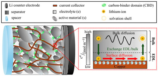
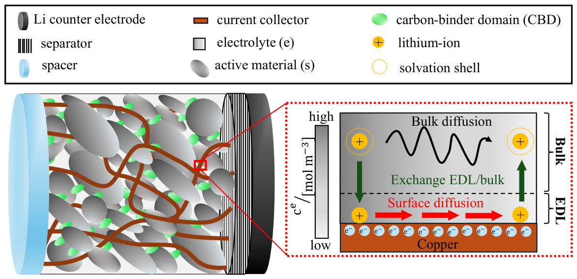
Beyond optimization of conventional foil-based electrodes, Zhang et al. [13] introduced a 3D nickel current collector fabricated using colloidal crystal templates as a sacrificial phase. Electrodeposition of a thin active material layer () onto the nickel nanostructure allows short solid-state diffusion lengths and well-interconnected pores, resulting in low tortuosity. Based on this strategy, Wang et al. [14] proposed a 3D copper fiber fleece as a current collector, fabricated by melt spinning and sintering. After coating the metal fiber fleece with graphite and carbon-binder domain (CBD), the electrode architecture was evaluated within a half-cell setup (see Figure 1). They demonstrated that due to improved electronic and ionic transport, the metal fleece enables significantly thicker graphite electrodes with lower electrolyte transport limitations. As schematically illustrated in Figure 1, this performance improvement is attributed to the breaking of ion-solvent complexes within the electrical double layer (EDL) adjacent to the metal fiber surfaces. As a result, ions move along the metal fiber surface with significantly higher mobility than in the bulk electrolyte, where the transport is hindered by the surrounding solvation shell. Furthermore, Wang et al. [14] experimentally demonstrated that a larger potential difference between the copper surface and the bulk electrolyte promotes the ion transfer from the bulk electrolyte into the EDL. The resulting activation of the high-mobility pathway enhances the effective ion diffusivity within the electrode.
Figure 1.
(Left): Graphite half-cell setup including the copper fiber fleece (orange), the spacer (light blue), the separator (hatched) and the lithium counter electrode (black). The porous graphite electrode consists of the active material (dark gray), the electrolyte (light gray) and the carbon-binder domain (CBD, green). (Right): Concept of the high-mobility pathway at the metal fiber fleece surface. The scheme shows a negatively charged surface, where lithium ions form the EDL. Solvated and desolvated lithium ions are shown in yellow. Adapted from reference [14].
Motivated by these findings, the present work focuses on the fiber-fleece concept proposed by Wang et al. [14]. Since the 3D metal fibers are electrochemically inactive, the central objective is to identify the optimal electrode architecture where the enhanced ion mobility overcompensates for the penalty from the inactive volume. For this purpose, computational modeling is used to investigate the underlying transport processes and systematically optimize the electrode architecture.
To capture the dynamics between electrolyte bulk and EDL, a variety of computational approaches exist. Molecular simulations resolve ion transport and interfacial phenomena at the molecular scale [14,15]. At the continuum scale, the Poisson-Nernst-Planck (PNP) model describes the interaction between ion transport and the electric field [16,17]. Assuming quasi-equilibrium, where ions are Boltzmann-distributed, the PNP equations reduce to the Poisson-Boltzmann (PB) model [18]. Due to their limitation to diluted solutions with point-like ions, both PNP and PB models are invalid for larger potentials [18,19], as typically present in lithium-ion batteries. To overcome this limitation, modified PNP [20,21] and modified PB models [19] have been developed, accounting for finite ion size and crowding effects, which are particularly relevant at higher potentials [22]. Since EDL models resolve the nanometer scale, they are too expensive to simulate complete porous electrodes. Cell-scale battery models, such as microscale [23,24], micro-macroscale [25,26] and macroscale models [27,28,29,30], in contrast, describe ion transport only in the bulk electrolyte and treat the current collector as inert. To our knowledge, no model links EDL ion transport at the metal fiber surface to the electrochemical performance of 3D fiber-fleece electrodes.
The aim of this work is to close this gap. To achieve this, a reduced version of the modified PB model is coupled with a surface diffusion mechanism and the parameters are fitted against the microfluidic channel experiments, reported in [14]. The resulting framework is then integrated into the pseudo-two-dimensional (P2D) model [27,31,32] as a source term at the metal fiber surface. This model is used to analyze and optimize the electrode thickness, fiber radius and the metal fiber volume fraction with respect to the volumetric energy and power density.
The first part of this work introduces the microfluidic channel experiment and presents the PB-surface diffusion framework together with the parameter fitting. The second part focuses on the coupling of this framework with the P2D model, which is used for parameter analysis and optimization of the 3D fiber-fleece architecture.
Use of Generative AI
Generative AI was used in the preparation of this work as follows:
- (i) Main manuscript. The content, data and scientific arguments were provided and developed by the authors. Claude (Anthropic) was used only to assist with wording and language editing of the authors’ text.
- (ii) Supplementary Materials. Claude (Anthropic) was used to assist with the text formulation of parts of the Supplementary Materials. The underlying content and data were provided by the authors.
No generative AI was used for the model development, simulations, data analysis or interpretation of results. All AI-assisted text was reviewed, verified and edited by the authors.
2. Quantification of the Electrical Double Layer Transport
The following section describes the workflow to quantify the enhanced ion transport of the electrical double layer. A model, combining the ion transport inside the electrolyte with a description of transport in the EDL, is proposed. This model is then compared with microfluidic channel experiments reported in literature [14], enabling the determination of the surface diffusivity.
2.1. Experiment
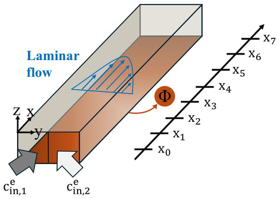
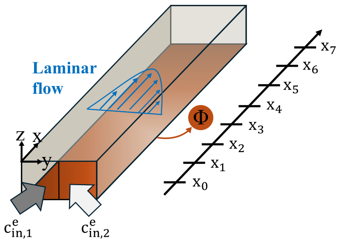
To measure the enhanced ion diffusivity within the EDL near the metal fiber surface, Wang et al. [14] developed a microfluidic channel with a rectangular cross-section, shown in Figure 2. Two electrically grounded electrolyte streams with different concentrations ( and in a mixture of 50:50 ethylene carbonate (EC) and dimethyl carbonate (DMC)) flow over a polarizable copper surface. The concentration difference between the -rich and -poor streams induces a diffusive flux in y-direction, driving lateral concentration mixing.
Figure 2.
Microfluidic channel with length , width and height . The length L, width W and height H correspond to the geometrical extents in x-, y- and z-direction. The parabolic laminar velocity profile is shown in blue. At (left-hand side), the -rich stream enters the channel, whereas at (right-hand side), the -poor stream enters. The applied metal potential is abbreviated as .
The flow rates of both streams are equal and set to satisfy the following two competing requirements: (i) They must be sufficiently low to ensure laminar flow, preventing turbulent mixing of the streams upon first contact and allowing continuous lateral mixing along the channel length in x-direction. (ii) The flow rates must be high enough to maintain convection-dominated transport in x-direction (high Péclet number ). Both requirements ensure that lateral mixing is governed purely by diffusion in y-direction.
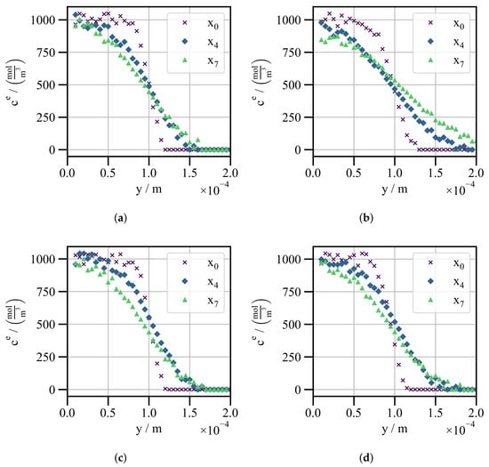
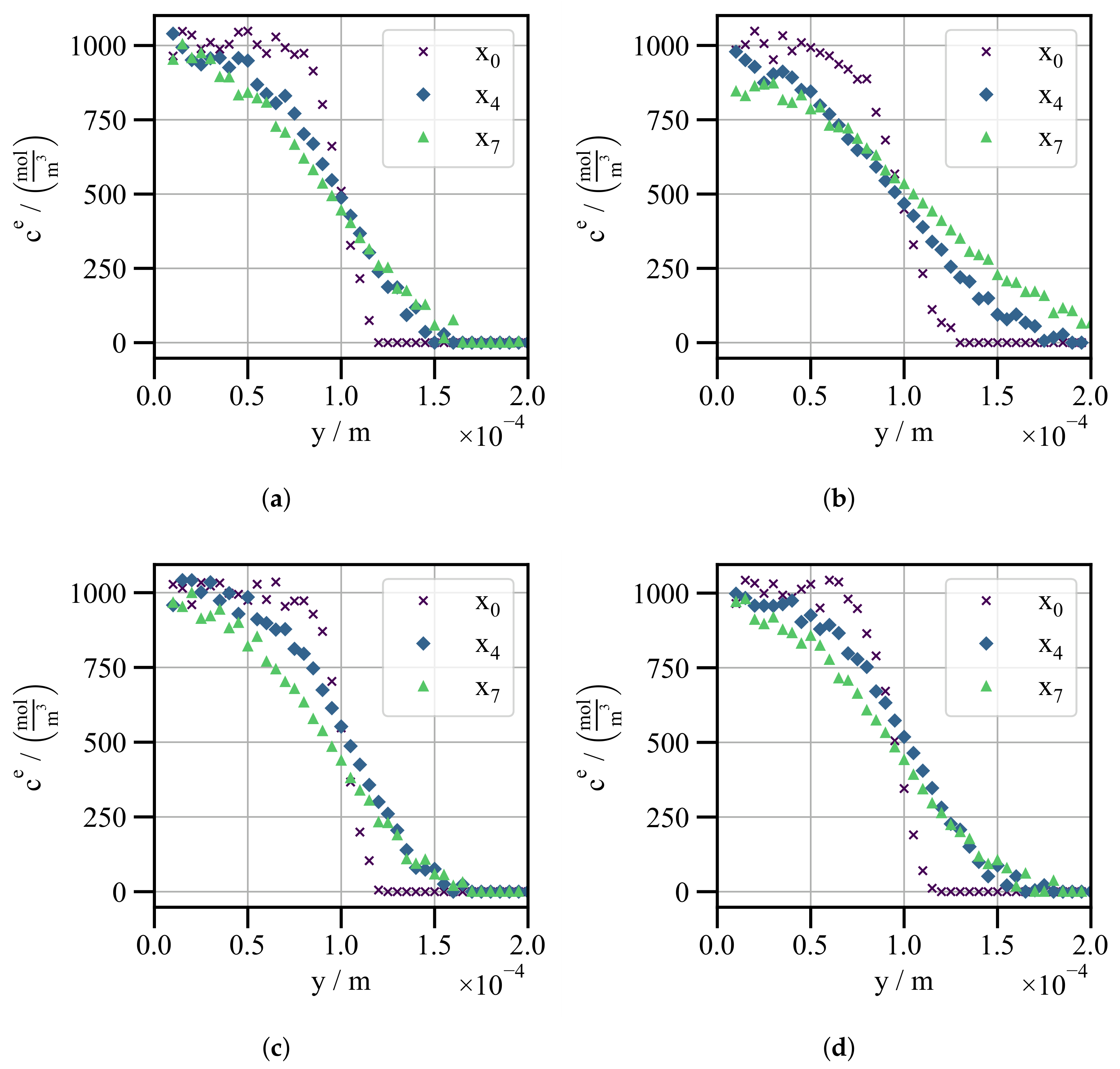
The lateral mixing of the electrolyte concentration profiles is measured by Raman spectroscopy across the full channel width at discrete positions to , separated by in the flow direction. Figure 3 shows the measured concentration profiles at channel heights of for different potentials applied to the copper surface ( and against the potential of zero charge). For clarity, only the profiles at positions are displayed.
Figure 3.
Measured electrolyte concentration across the channel width in y-direction at discrete downstream positions (purple cross markers), (blue diamond markers) and (green triangular markers). The concentration profiles are shown for two channel heights and two applied potentials: (a) , . (b) , . (c) , . (d) , .
Figure 3a displays the concentration profiles at a height of and an electrically neutral copper surface (). As shown for position , there are already pronounced concentration gradients, as the two streams first come into contact upstream of this position at . Even at position , the concentration remains far from complete mixing and still exhibits steep gradients, which serve as a sensitive window for fitting. Increasing the potential from to leads to faster lateral mixing between the -rich and -poor regions (see Figure 3b). This effect is attributed to the potential , which activates the high-mobility pathway in the EDL, resulting in an enhanced effective diffusivity compared to the electrically neutral scenario .
Figure 3c,d show the corresponding concentration profiles at a larger channel height of . At , increasing the channel height has no effect on lateral mixing (see Figure 3c), as the high-mobility pathway in the EDL is inactive and transport is governed only by bulk electrolyte diffusion. As depicted in Figure 3d, a higher applied potential again accelerates lateral mixing. However, compared to , the acceleration is less pronounced, as the larger distance from the copper surface increases the relative contribution of the bulk electrolyte. As a result, the effective diffusivity is reduced.
Figure S1 in the Supplementary Materials presents the remaining data sets for the intermediate height and applied potentials . At positive potentials , mixing is faster than at but slower than at , since the anions form the EDL and travel along the surface while bulk electroneutrality forces the lithium ions to follow (Figure S8 in [14]).
2.2. Model
To predict the lateral mixing at different channel heights and potentials, the model framework in Table 1 is employed. It captures the interaction between the slow bulk diffusion and the high-mobility pathway in the EDL, illustrated in Figure 1.
Table 1.
Coupled bulk and EDL transport model: convection-diffusion in the bulk electrolyte and surface diffusion along the copper surface.
2.2.1. Electrolyte Bulk
The ion transport in the bulk is described by the electrolyte mass transport equation of Latz and Zausch [23], including convection. Assuming electroneutrality, the two-ion transport problem can be reduced to a single effective interdiffusion coefficient , denoted here as the electrolyte bulk diffusivity. Since the electrolyte is electrically grounded, migration is neglected and the ion transport is described by the convection-diffusion model (see Equation (2)). For a fully developed laminar flow, the velocity field is given by Equation (6), which depends on the average velocity , the channel width W and the channel height H.
The parabolic velocity profile assumes laterally uniform viscosity. Since the two streams differ in electrolyte concentration and thus in viscosity, the measured concentration profiles must be normalized. Details of this normalization step are provided in Section S1 of the Supplementary Materials.
According to Figure 2, at the inlet (), we set the Dirichlet boundary condition, given in Equation (7):
At the outlet (), a zero-gradient Neumann boundary condition (see Equation (8))
is applied, corresponding to a purely convective outflow. All remaining boundaries, except for the copper surface, are treated as no-flux boundaries. At the copper surface, the mass transfer is defined by a sink/source term R, which represents the ion exchange with the EDL (see Equation (3)).
2.2.2. EDL
Since the EDL extends only over nanometer length scales, while the bulk electrolyte transport occurs on the micrometer scale, a fully coupled multiscale simulation is computationally demanding. For that reason, as outlined in the introduction, a reduced version of the modified PB model is employed to describe the ion exchange R between the EDL and the bulk electrolyte.
Following the approach of Chu et al. [33,34], the EDL can be considered as an effective boundary condition, as its thickness is negligible compared to the electrolyte bulk size. In this so-called thin double layer limit, the ion concentration reduces to the excess surface concentration of cations (+) or anions (−),
which is obtained by integrating the difference between the ion concentration in the EDL and the adjacent bulk electrolyte concentration across the EDL thickness.
According to the Gouy-Chapman-Stern model, the EDL consists of the Stern layer (inner and outer Helmholtz planes) and the diffuse layer. In the present work, only the diffuse layer is considered, while the Stern layer and its associated linear potential drop are neglected.
For this reason, the electrostatic potential of the diffuse layer can be defined relative to the bulk condition as
The EDL potential extends from the applied surface potential at the copper surface to in the bulk electrolyte. Since the electrolyte streams are electrically grounded, the bulk potential is . Although more accurate descriptions of the diffuse layer are available, the modified Poisson-Boltzmann model is employed to represent the ion distribution within the diffuse layer [19,35]. The motivation is to adopt a computationally efficient model whose predictive performance is enhanced by calibration against experimental data. Assuming a symmetric, binary electrolyte with ions and solvent molecules of the same size, the modified Poisson-Boltzmann model relates the EDL potential to the concentration of cations (+) or anions (−) under quasi-equilibrium conditions.
As shown in Equation (11), depends on the bulk electrolyte concentration , the ion valence , the Faraday constant , the universal gas constant , the temperature T and the dimensionless steric parameter . The numerator corresponds to the classical Boltzmann distribution and describes the dependence of ion concentration on the electrostatic energy. The denominator, containing the dimensionless steric parameter , considers steric effects due to the finite ion size and limits the ion concentration at high potentials .
According to Equation (12), the dimensionless steric parameter depends on , the Avogadro constant and the effective ion size a, which determines the maximum achievable ion concentration [19].
As discussed after Figure 3, enhanced transport occurs for both signs of , with cations forming the EDL at negative and anions at positive potentials. In the modified Poisson-Boltzmann model, the concentration ratio of cations to anions in the EDL is given by . Already at , this ratio reaches approximately , so the anion concentration is negligible compared to the cations, and vice versa at . For that reason, we define the effective ion concentration as
which is independent of the ion species forming the EDL and symmetric in (for equal ion sizes as assumed for ). Integrating Equation (13) over the EDL space according to Equation (9) results in the effective excess surface concentration in quasi-equilibrium :
Using the symmetry in , the arguments of the exponential and sinh in Equation (11) can be replaced by their absolute values. Application of the chain rule allows integration over the EDL potential instead of over the EDL space (see Equation (14)). Using the definition of in (Equation (27) in [19]), the quasi-equilibrium excess surface concentration can be written, in a form similar to (Equation (54) in [34]), as
where denotes the Debye length, and and are the vacuum and relative permittivity, respectively.
This expression of is used in the sink/source term (see Equation (4) in Table 1), where the ion exchange rate R is driven by the deviation between the quasi-equilibrium excess surface concentration and the actual excess surface concentration . The rate constant is approximated as the inverse of the Debye time (see Equation (16)) [18], which describes how fast the EDL approaches its quasi-equilibrium state after a perturbation:
Here, denotes the ionic conductivity of the bulk electrolyte. The characteristic relaxation time of the EDL is typically much smaller than the characteristic time scales of the bulk electrolyte transport. For that reason, normally the EDL is assumed to remain in quasi-equilibrium, allowing direct description by without the evolution approach in Equation (4).
However, since the high-mobility pathway in the EDL is described by a surface transport equation, the quasi-equilibrium excess surface concentration cannot be used directly as a variable, as it represents a static equilibrium state without surface transport. For this reason, we consider the actual excess surface concentration as a dynamic variable, allowing surface transport along the metal surface. The large value of ensures that remains close to its corresponding quasi-equilibrium state .
According to the surface transport equation (see Equation (5) in Table 1), ions accumulate in the EDL due to surface mass transfer with the surface diffusivity and the exchange with the bulk electrolyte by the sink/source term R. Compared to the approach of Chu et al. [33], the ion migration is neglected in the present surface transport equation to improve the determination of the parameters. Under this assumption, the effective ion size a and the surface diffusivity are the only fitting parameters governing the EDL transport.
2.3. Empirical Fitting
For the empirical fitting, the model framework (see Table 1) is solved on the channel geometry, shown in Figure 2, using the finite-element simulation software COMSOL Multiphysics® (version 6.3). The fully coupled transport equations are solved using the direct solver PARDISO and implicit BDF time integration with adaptive step size (relative tolerance , maximum order 5). A mesh sensitivity analysis is performed for a channel height of and an applied potential of , as this is the scenario with the strongest lateral mixing. The geometry is discretized using 45360 hexahedral mesh elements. Further details on the mesh sensitivity analysis are provided in Section S2 of the Supplementary Materials.
Based on this numerical setup, simulations are carried out for each experimental scenario with varying channel heights H and applied potentials using the parameters, summarized in Table 2.
Table 2.
Specifications of the channel experiment and transport parameters utilized for the determination of surface diffusivity.
As shown in Table 2, two values are considered for the relative permittivity . Since the solvent composition within the EDL may differ from the electrolyte bulk composition, simulations are performed with pure dimethyl carbonate ( [37]) and a 50:50 mixture of EC and DMC corresponding to bulk composition ( [38]).
Since the integral in Equation (15) cannot be solved analytically, it is evaluated numerically prior to the simulation to generate a lookup table for the quasi-equilibrium excess surface concentration . The table covers the dependence on the effective ion size a, the bulk concentration and the applied potential to the copper surface .
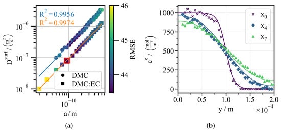
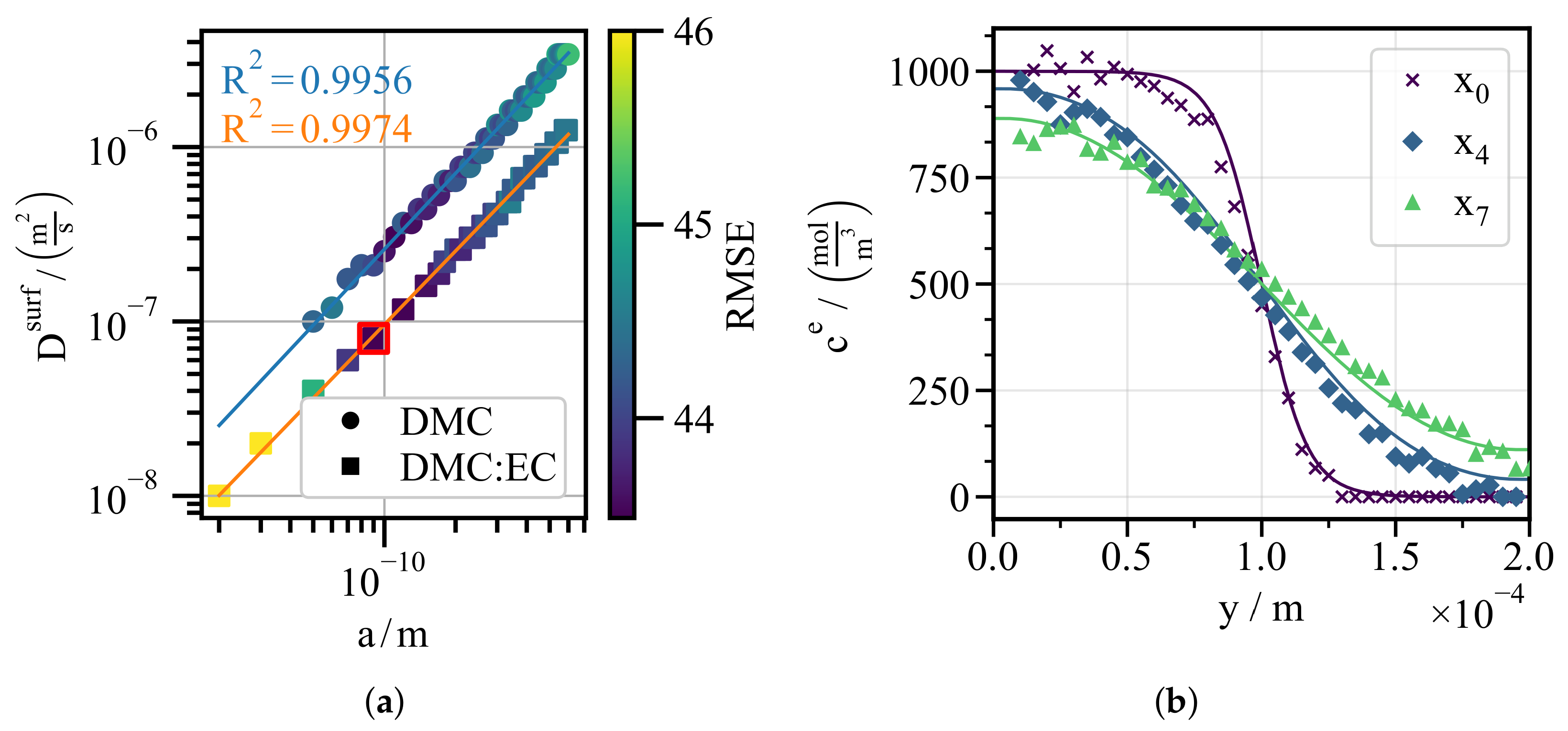
As shown in Figure 4a, due to the lack of identifiability of the effective ion size a, the surface diffusivity is fitted over a range of a. This range spans from the ionic radii of the bare ions (, [39]) to the solvated radii, such as the Stokes radius of in EC/DMC ( [40]). As a fitting metric, the root mean square error
is evaluated for all experimental data sets with varying channel height H and applied potential at all positions . With an overall average of approximately compared to an average electrolyte concentration of , the RMSE indicates good agreement between the model and the experiment. Figure 4a illustrates two data sets corresponding to different values of the relative permittivity . With for both cases, the relation between a and can be considered linear in logarithmic space.
Figure 4.
(a) Linear relationship between the fitted values of the effective ion size a and the surface diffusivity for DMC (circle markers) and DMC:EC (square markers). The color map represents the root mean square error (RMSE) between the experimental and simulated results. (b) Comparison between measured and simulated profiles for and .
Figure 4b compares the experimental data ( and , see Figure 3b) with the simulated concentration profiles. The simulation uses the red-marked parameter set with an effective ion size of and the fitted surface diffusivity for , chosen as a representative pair within the investigated range of a. The other combinations provide equally good fits. Even if a larger effective ion size reduces the quasi-equilibrium excess surface concentration through steric effects, the correspondingly higher fitted compensates, so that the resulting surface flux is maintained. The neglect of the Stern layer is therefore acceptable, as its contribution is absorbed into the fitted surface diffusivity. Since a reliable identification of a would require additional experiments, this parameterization is considered sufficient for the present work, which focuses on establishing a methodology for the optimization of the metal fiber architecture. The sensitivity of the results to the choice of the parameter pair is analyzed in Section S5 of the Supplementary Materials for and (Stokes radius of ), representing the lower and upper ends of the investigated range with their correspondingly fitted surface diffusivities.
3. Metal Fiber Optimization
To optimize the metal fiber architecture, an electrochemical model is required which accurately captures the relevant transport processes while maintaining low computational cost. Therefore, the fitted EDL model framework is coupled with a macroscopic battery model, such as the pseudo-two-dimensional (P2D) model.
3.1. Methodology
3.1.1. Half-Cell Model
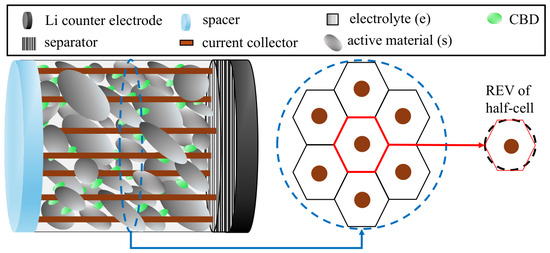
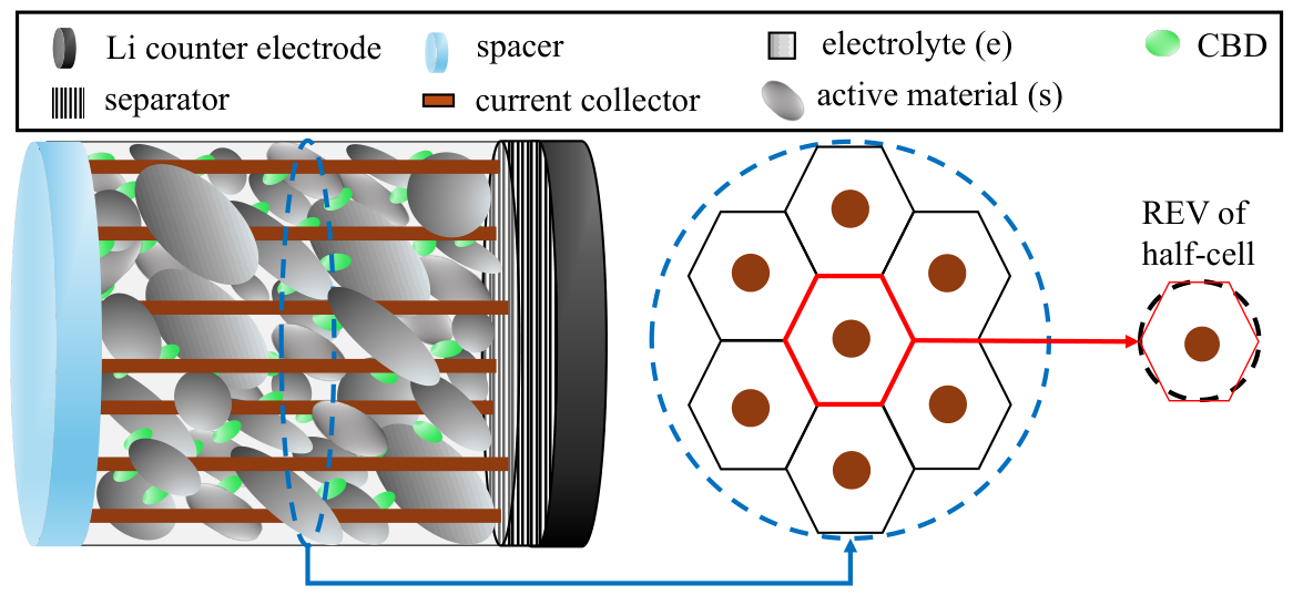
For the sake of simplicity, the fiber-fleece architecture of the half-cell, shown in Figure 1, is reduced to a uniform distribution of straight, cylindrical metal fibers, which extend from the blue spacer to the hatched separator (see left part of Figure 5). The uniform distribution enables the partition of the cross-sectional area into one hexagonal unit cell per fiber (see center of Figure 5). This partitioning becomes more accurate as the fiber number density increases. Each hexagonal unit cell is further approximated by a cylinder, which serves as the representative elementary volume (REV) of the half-cell geometry (see right part of Figure 5).
Figure 5.
(Left): Simplified half-cell geometry with uniformly distributed, straight copper fibers (orange), spacer (light blue), separator (hatched) and lithium counter electrode (black). Each copper fiber is surrounded by the porous electrode, which consists of active material (dark gray), electrolyte (light gray) and the CBD (green). (Center): Partitioning of the cross-sectional area (dashed blue circle) into hexagonal unit cells, one per fiber. (Right): Approximation of the red-highlighted hexagonal unit cell by a cylinder (dashed black contour), which represents the REV of the half-cell geometry.
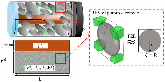
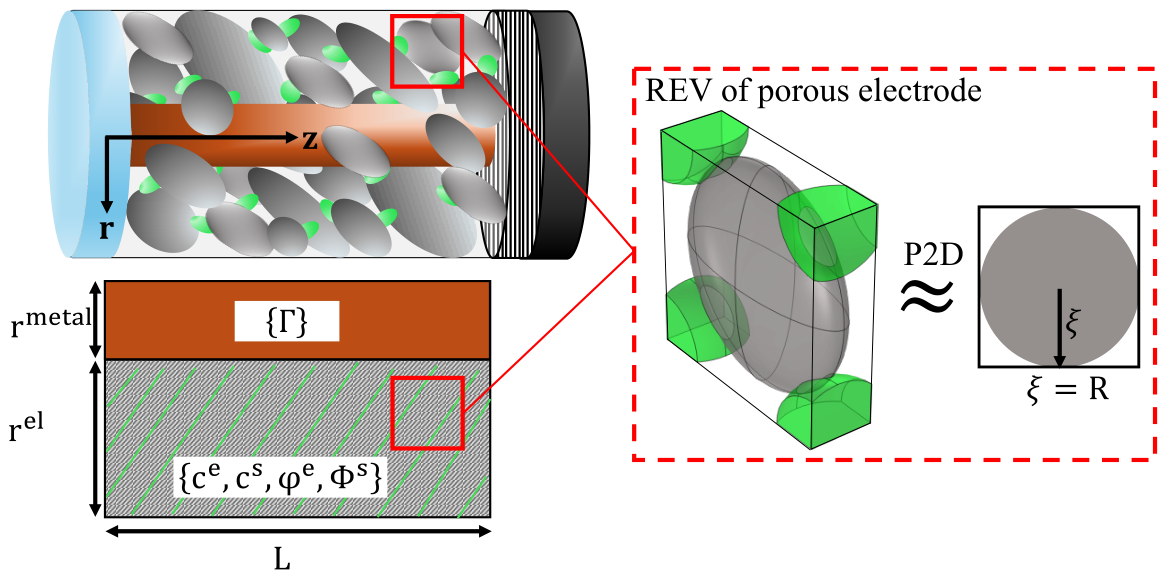
Figure 6 shows the cylindrical REV of the half-cell geometry, comprising one cylindrical metal fiber and the surrounding graphite electrode. The porous electrode, consisting of the graphite active material (superscript s), the carbon-binder domain (CBD) and the electrolyte (superscript e), is treated as a quasi-homogeneous continuum. Since the REV is radially symmetric, the 3D problem can be reduced to a 2D axis-symmetric domain, defined by the electrode thickness L, the fiber radius and the outer electrode radius . As shown in Figure 6, we consider an REV of the porous electrode, in which the graphite particles are approximated as ellipsoids coated by the CBD. The resulting anisotropy is a characteristic of foil-based graphite electrodes, as the calendering process enhances the effective transport in radial direction, while reducing the transport in the axial z-direction [41]. The same microstructure is assumed for the fiber-fleece electrode for consistency of comparison. Based on these anisotropic effective properties, the P2D model employs volume-averaged transport equations to describe the transport of the electrolyte concentration , the electrolyte potential and the solid-phase potential within the homogeneous porous electrode. In the electrolyte phase, mass and charge transport (see Equations (18) and (19) in Table 3) are governed by the Nernst-Planck equation under the assumption of electroneutrality, using the effective electrolyte diffusivity , the effective ionic conductivity , the transference number and the porosity . The solid-phase potential is described by Ohm’s law (see Equation (20) in Table 3) using the effective electronic conductivity .
Figure 6.
(Top Left): 3D cylindrical REV of the half-cell geometry comprising a straight copper fiber (orange), the spacer (light blue), the separator (hatched) and the lithium counter electrode (black). The copper fiber is surrounded by the porous electrode, which consists of active material (dark gray), electrolyte (light gray) and the CBD (green). (Bottom Left): 2D axis-symmetric domain which consists of the copper fiber () and the porous electrode (). The porous electrode is treated as a quasi-homogeneous continuum. (Right): Representative elementary volume (REV) of the quasi-homogeneous porous electrode and its spherical approximation used in the P2D model.
Table 3.
Volume-averaged transport equations of the P2D model [27,31,32]. The CBD is included in the effective transport equations, with lithium-ion transport assigned to the electrolyte and electronic conductivity to the active material. The effective molar ion flux in the electrolyte is defined in Equation (18).
Due to volume-averaging, all transport equations include the Butler-Volmer current density [27] (see Equation (21)) as a reaction source or sink term, where denotes the specific interfacial area of the electrochemically active interface in the porous-electrode REV.
In Equation (21), refers to the maximum lithium concentration, k to the Butler-Volmer rate constant and to the open-circuit voltage.
As illustrated in Figure 6, the P2D model approximates the ellipsoidal graphite particles in the REV by equivalent spherical particles without overlap and without CBD coating. The lithium concentration in the active material is described by radial solid-phase diffusion [27], characterized by the diffusivity (see Equation (22)):
Since the symbol r is already used for the radial coordinate of the cylindrical half-cell REV, we introduce for the radial coordinate in the spheres. Due to spherical symmetry, the following boundary condition applies at the particle center :
At the electrochemically active interface , the diffusive mass transfer is defined by the Butler-Volmer current density:
The determination of the geometrical and effective transport parameters, including the fitting of an equivalent spherical radius to the ellipsoid in the REV, is provided in Section S3 of the Supplementary Materials. The initial and boundary conditions of the half-cell geometry are described in Table A1 in Appendix A.
To capture the high-mobility pathway at the metal fiber surface , the electrolyte concentration of the P2D model is coupled to the EDL model framework described in Table 1 (Equations (4) and (5)). In contrast to the previous section, the bulk concentration is substituted by the volume-averaged concentration . Because the electrolyte is not electrically grounded and the metal fiber potential corresponds to the solid-phase potential, the potential difference replaces the applied potential as the input to the quasi-equilibrium excess surface concentration. Since is reported versus Li/Li+ rather than the potential of zero charge used to define , must be shifted according to
before entering . To our knowledge, of copper in EC/DMC with has not been reported. From the measurements of Fujieda et al. [42], a value of vs. Li/Li+ can be derived for copper, but their electrolyte differs in both solvent and conducting salt, introducing considerable uncertainty. Since this work focuses on establishing an optimization methodology for the metal fiber architecture, vs. Li/Li+ is assumed for simplicity. The sensitivity of the model predictions to is analyzed in Section S5 of the Supplementary Materials, where we consider the literature value vs. Li/Li+.
To evaluate the performance of the 3D fiber-fleece architecture for optimization, the half-cell voltage is defined as the following potential difference
with the electrolyte potential set to zero due to the Dirichlet boundary condition (see Table A1).
Since copper has a high electronic conductivity (), charge transport in the fiber is not explicitly resolved and the fiber is treated as equipotential. As a result, the current enters through the porous electrode cross-section rather than the fiber. Section S7 of the Supplementary Materials confirms that the choice of current inlet does not affect the results.
3.1.2. Full-Cell Reconstruction
To obtain a realistic voltage window for the optimization, the graphite half-cell simulation is transformed into an equivalent full-cell representation by electrode balancing with a virtual NMC111 cathode and an aluminum foil current collector. Following Ahmed et al. [43], the cathode (subscript p) is assumed to possess a capacity that is lower by a factor of compared to the graphite anode (subscript n). Accordingly, the cathode capacity is given by
where denotes the graphite anode capacity, calculated from Faraday’s law. Here, is the anode thickness, the volume fraction of the graphite active material and the initial lithium concentration. The cross-sectional area of the porous graphite electrode, excluding the metal fiber contribution, is defined as:
In the next step, the concentration window between the initial concentration and the maximum concentration is adjusted according to the ratio of transferred charge to the cathode capacity (see Equation (29)).
For a galvanostatic operation, the transferred charge is given by the product of the elapsed time t and the applied current . Since the open-circuit voltage of the cathode is known, the full-cell voltage can be reconstructed from the simulated anode voltage under the assumption of negligible transport limitations in the cathode (see Equation (30)).
3.2. Results and Discussion
To optimize the metal fiber architecture, the graphite electrode thickness , the metal fiber radius and the metal fiber volume fraction are treated as design parameters, while all remaining parameters are chosen according to Table A2 in Appendix A. First, one reference case is simulated to illustrate the underlying physics. Second, the sensitivity of the design parameters with respect to the optimization objective is analyzed. Finally, the optimization is performed for fixed values of .
The graphite half-cell model is implemented in COMSOL Multiphysics® (version 6.3) using the settings, described in the previous section, with a relative tolerance of . All simulations are terminated when either the cut-off voltage reaches or the electrolyte concentration drops below . The mesh sensitivity analysis, performed for the reference case, is provided in Section S4 of the Supplementary Materials.
3.2.1. Reference Case
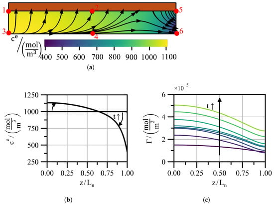
Figure 7a illustrates the half-cell setup of the reference case with an electrode thickness of , a metal fiber radius of , a metal fiber volume fraction of and a discharging rate of .
Figure 7.
(a) 2D axis-symmetric domain of the reference case including the metal fiber (orange) and the porous electrode. The colormap shows the electrolyte concentration at the terminal time , with yellow and purple indicating high and low concentrations, respectively. The streamlines indicate the ion flux into and out of the EDL at the metal fiber surface. The points 1–6 serve as reference locations for the line plots. (b) Electrolyte concentration along line at and . (c) Temporal evolution of the excess surface concentration along line , with green indicating high and purple low values of .
During discharging, lithium deintercalates from the graphite active material and the released ions move toward the separator. As indicated by the streamlines, about half of the ions preferentially follow the high-mobility pathway in the EDL at the metal fiber surface (line between points 1 and 5) rather than the tortuous pore path through the porous electrode. The resulting stationary distribution of the electrolyte concentration , shown as a colormap, exhibits a steep gradient in z-direction and is nearly uniform in the radial direction r.
Figure 7b compares the initial uniform electrolyte concentration profile with the stationary profile along the line between points 3 and 6, highlighting the build-up of the concentration gradient caused by the imposed flux boundary condition at the right boundary (line between points 5 and 6).
As shown in Figure 7c, the excess surface concentration along the metal fiber surface increases during discharging. This can be attributed to the increasing solid-phase potential , which results in a higher quasi-equilibrium excess surface concentration . Depending on and the surface diffusivity , the resulting profiles exhibit a characteristic concentration gradient that drives surface diffusion of the ions toward the separator.
To quantify the contribution of the high-mobility pathway in the EDL, we introduce the dimensionless number , in analogy to the dimensionless number in [44] and the Bikerman number in [19,33]. defines the ratio between the axial surface flux along the high-mobility path (see Equation (5)) and the axial flux through the porous electrode (see Equation (18)):
The specific metal fiber surface area follows directly from the radii and :
To enable comparison across different half-cell geometries, is averaged over time and space. Spatially, is averaged along the radial segment between points 2 and 4 and is evaluated at point 2. For the reference case, the time- and space-averaged value is . This corresponds to a surface flux share of , so about half of the ions use the high-mobility pathway.
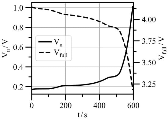
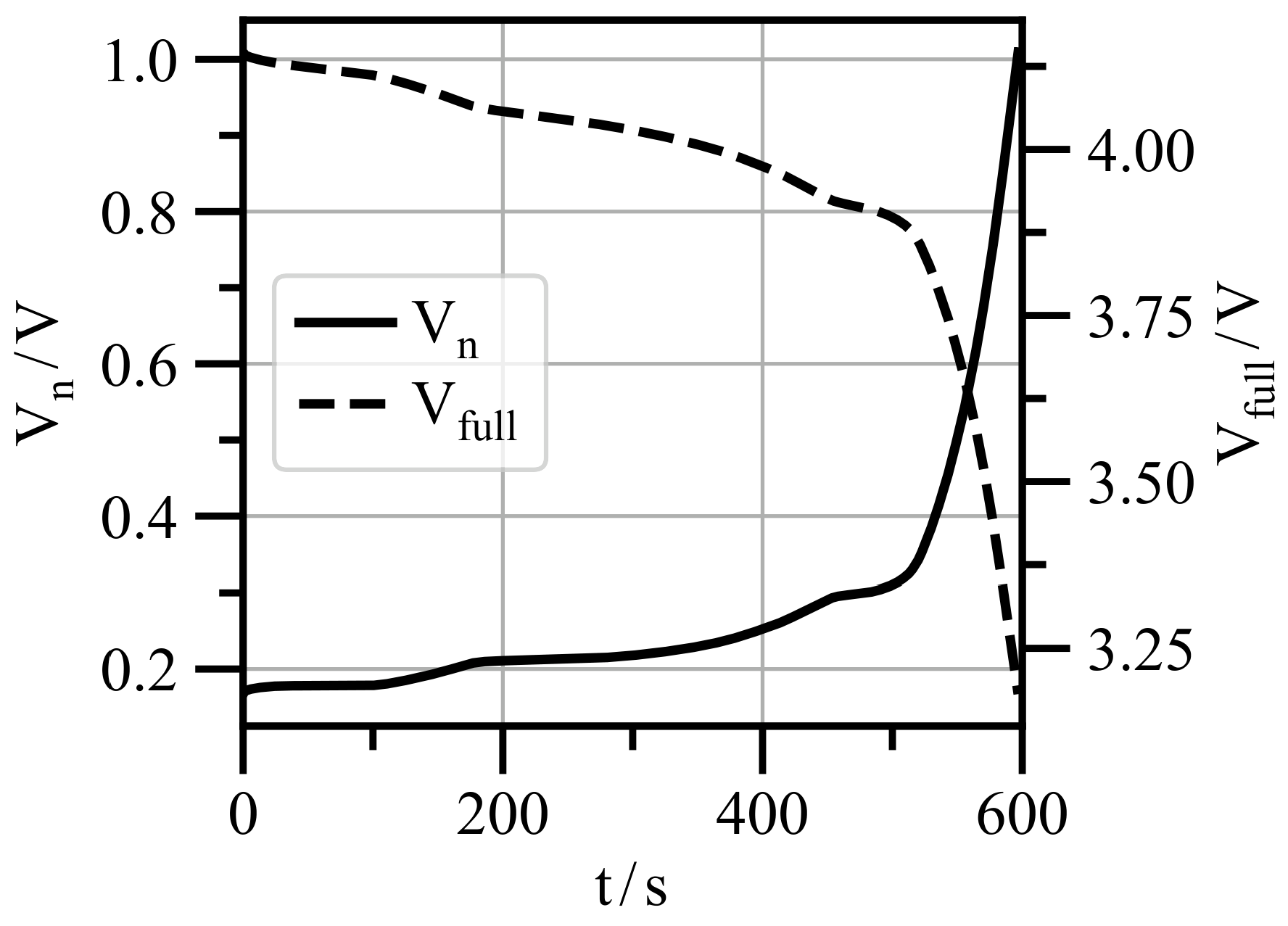
Figure 8 shows the half-cell voltage versus Li/Li+ which corresponds to the solid-phase potential (see Equation (26)) and thus to the metal fiber potential . starts at and rises until the cut-off voltage of is reached.
Using Equation (30), the NMC111/graphite full-cell voltage is reconstructed, resulting in a voltage window between and . Since the full-cell reconstruction assumes a cathode without transport limitations, cathodic overpotentials are neglected and is overestimated relative to a real full cell (see Section S6 of the Supplementary Materials).
To perform the optimization of the 3D fiber-fleece architecture, the reconstructed full-cell voltage is used to determine the volumetric energy density and volumetric power density , which serve as optimization objectives. To evaluate these volumetric quantities, the full-cell volume must be determined. For this reason, the thickness of the virtual NMC111 cathode is derived from the cathode capacity according to
where denotes the active material volume fraction, the maximum lithium concentration of the active material and the initial lithium concentration. Compared to the calculation of the anode capacity in Equation (27), the electrode cross-sectional area is replaced by the total cross-sectional area for the virtual cathode, as a conventional aluminum foil is used instead of the 3D fiber-fleece current collector. Knowing the full-cell volume, the volumetric energy density is determined by the following integration over the discharge time :
where the applied current is determined from the nominal anode capacity and the corresponding C-rate. denotes the aluminum foil thickness of the virtual cathode and the copper foil thickness of the anode. In fiber-based electrodes, the copper fibers replace the copper foil () and their volume is already contained in the anode volume. For metal fiber volume fractions , the electrode is treated as a conventional foil-based electrode with . The corresponding time-averaged volumetric power density is calculated as
Since cathodic overpotentials are neglected, the determined volumetric energy and power densities and represent an upper bound for a complete cell. For the reference geometry, a full-cell simulation shows that the reconstruction overestimates by to in the operating regime without electrolyte depletion (Section S6 of the Supplementary Materials).
3.2.2. Parameter Analysis
As preparation for the optimization, the sensitivity of and to the design parameters is investigated by varying the C-rate, the anode thickness , the metal fiber radius and the metal fiber volume fraction around the reference case (, , and ). Each modification of the reference electrode geometry requires an adaptation of the cathode thickness according to the electrode balancing assumption for the full-cell reconstruction in Equations (27) and (33).
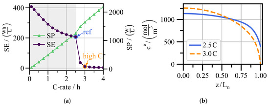
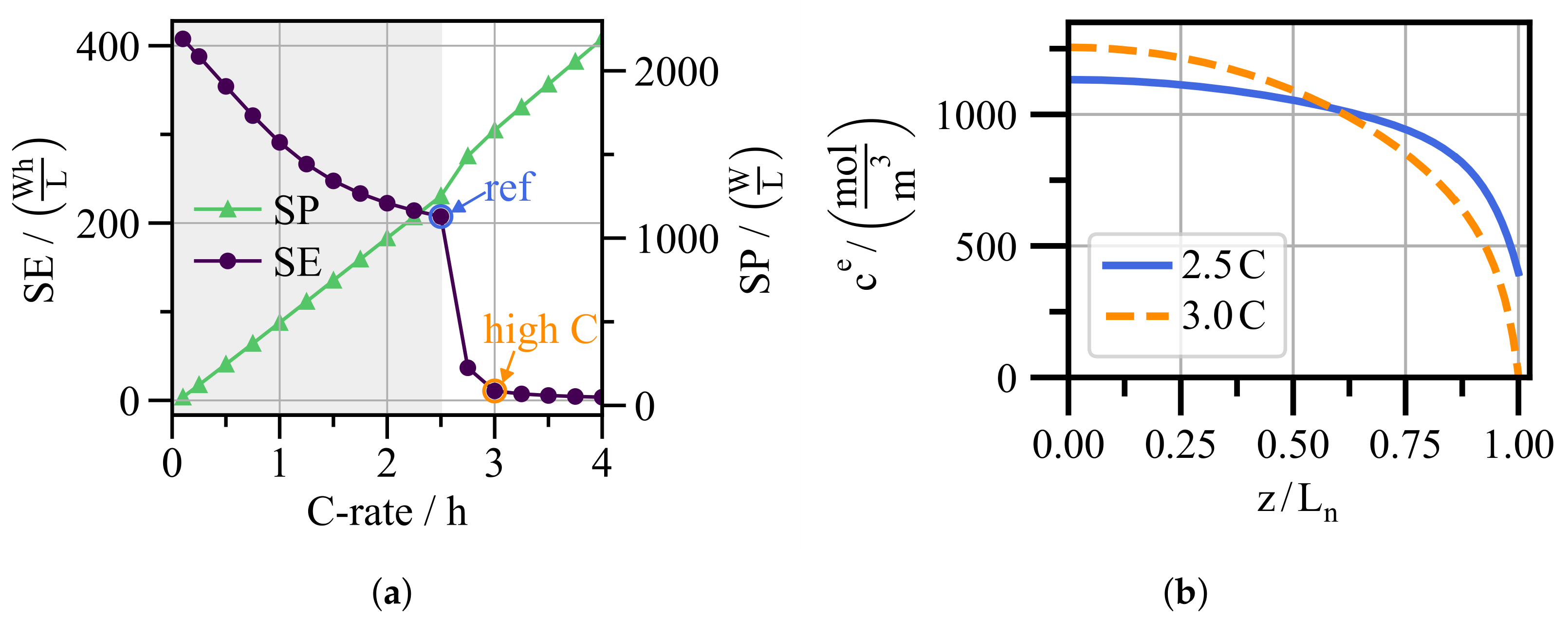
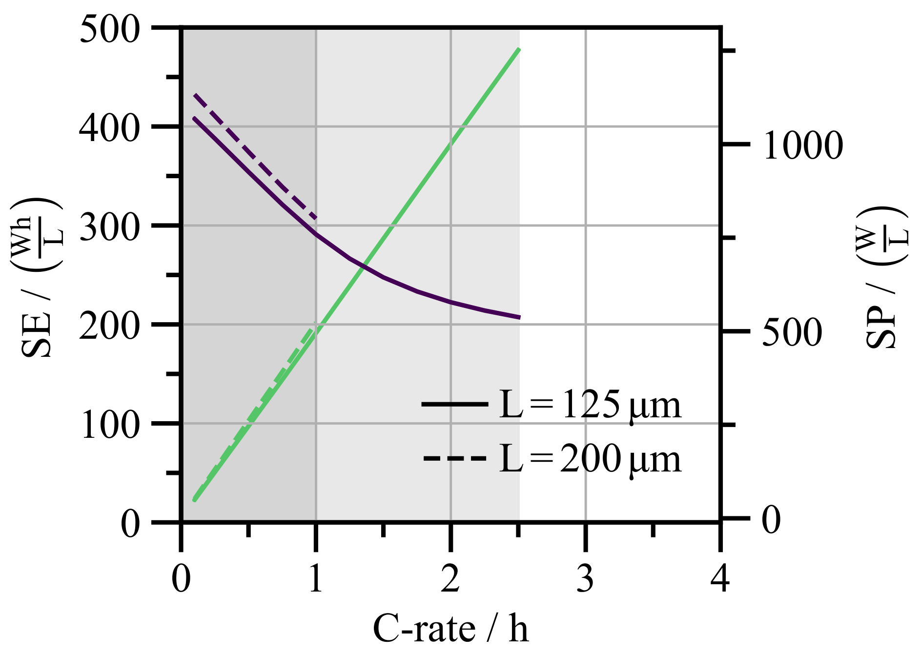
C-rate—To evaluate the effect of the C-rate on and , the C-rate is varied from to for the reference electrode geometry (see Figure 9a). At low C-rates, transport limitations are negligible, allowing full utilization of the available energy density (~). Increasing the C-rate toward the blue-marked reference case with , starts to decrease as solid-phase diffusion limitation becomes relevant. At higher C-rates, and thus higher current densities, the solid-phase diffusivity is no longer sufficient, leading to an increasing concentration deviation between particle interior and surface. This results in a higher overpotential and a lower . Further details on this limitation are discussed in [30].
Figure 9.
(a) Volumetric energy density (purple circle markers) and volumetric power density (green triangular markers) as a function of the C-rate for the reference geometry (solid line). The reference C-rate () is marked in blue, while the higher C-rate of is marked in orange. The gray band marks the operating regime without electrolyte depletion, defined by . (b) Electrolyte concentration along line at for both highlighted C-rates.
To achieve higher power densities, a further increase in C-rate is required. This leads to a pronounced decrease in , which is caused by electrolyte transport limitations. To illustrate this limitation, Figure 9b compares the stationary electrolyte concentration profile of the reference case (see Figure 7b) with the orange-marked simulation scenario exhibiting electrolyte diffusion limitation. While the gradients of the electrolyte concentration in the reference case remain moderate, the increased current demand at higher C-rates results in steep concentration gradients despite the high-mobility pathway at the metal fiber surface. As a result, approaches zero near the separator, indicating electrolyte depletion.
Since the resulting low values of are insufficient for mobility or industrial applications, the following analysis focuses on the gray-marked operating regime without electrolyte depletion.
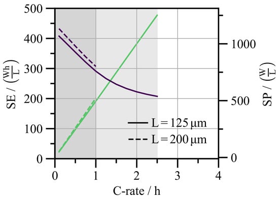
Electrode thickness—To investigate the effect of the electrode thickness, Figure 10 compares the reference geometry with a thicker electrode of while keeping the metal fiber radius at and the metal fiber volume fraction at . For clarity of comparison, the individual C-rate markers are omitted in the following.
Figure 10.
(purple) and (green) as a function of the C-rate for the reference geometry (solid lines) and for the thicker electrode (dashed lines). The operating regime without electrolyte depletion is highlighted in light gray for the reference geometry and dark gray for the thicker electrode.
At low C-rates, the thicker electrode achieves a higher value of compared to the reference geometry. This improvement comes from the larger electrode thickness which reduces the relative fraction of electrochemically inactive components, such as the separator and the aluminum current collector. In the introduction, this is referred to as the inactive volume penalty.
However, the longer ion transport path through the thicker electrode causes pronounced electrolyte diffusion limitation, leading to depletion already at 1 C. Both increasing electrode thickness at a fixed C-rate and increasing the C-rate at a fixed electrode thickness lead to electrolyte diffusion limitation.
Since both the C-rate and the volumetric power density scale with the electrode thickness, the two electrodes exhibit similar values. However, the operating regime without electrolyte depletion is limited to lower C-rates for the thicker electrode, which results in lower maximum compared to the reference geometry.
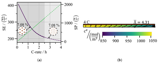
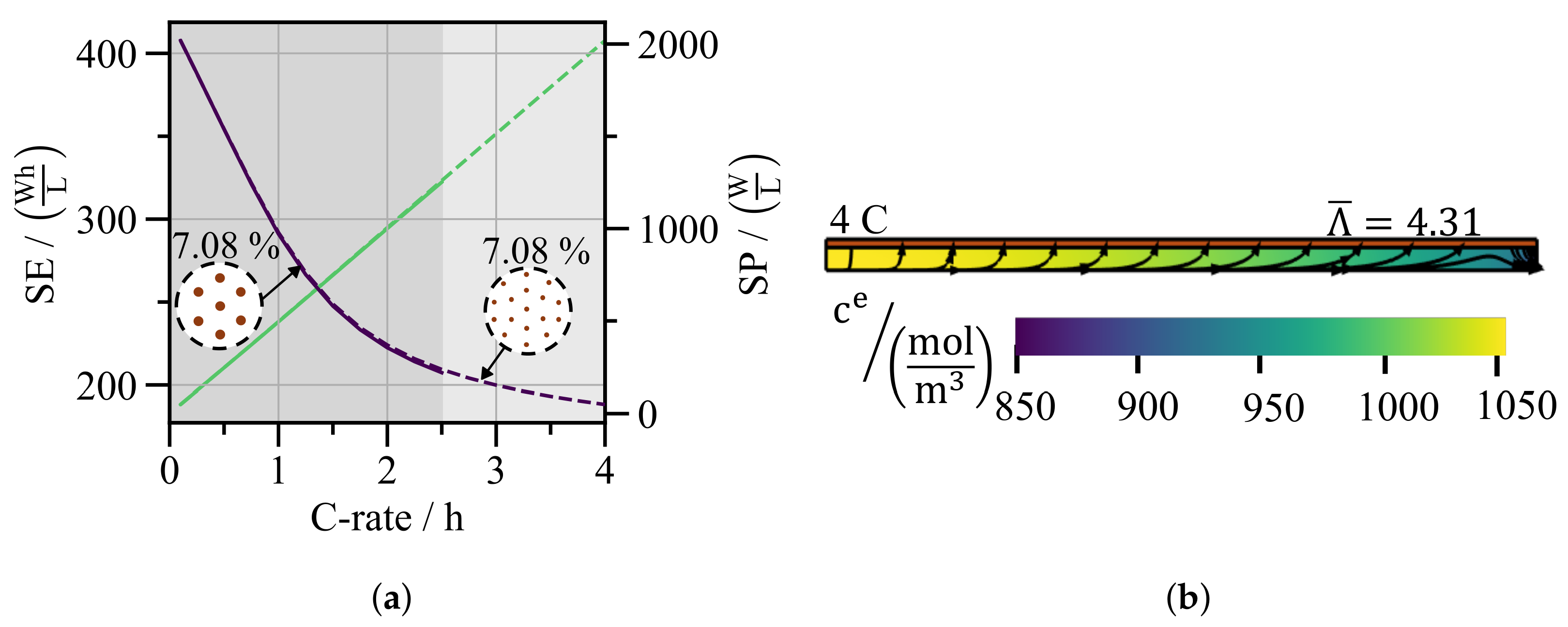
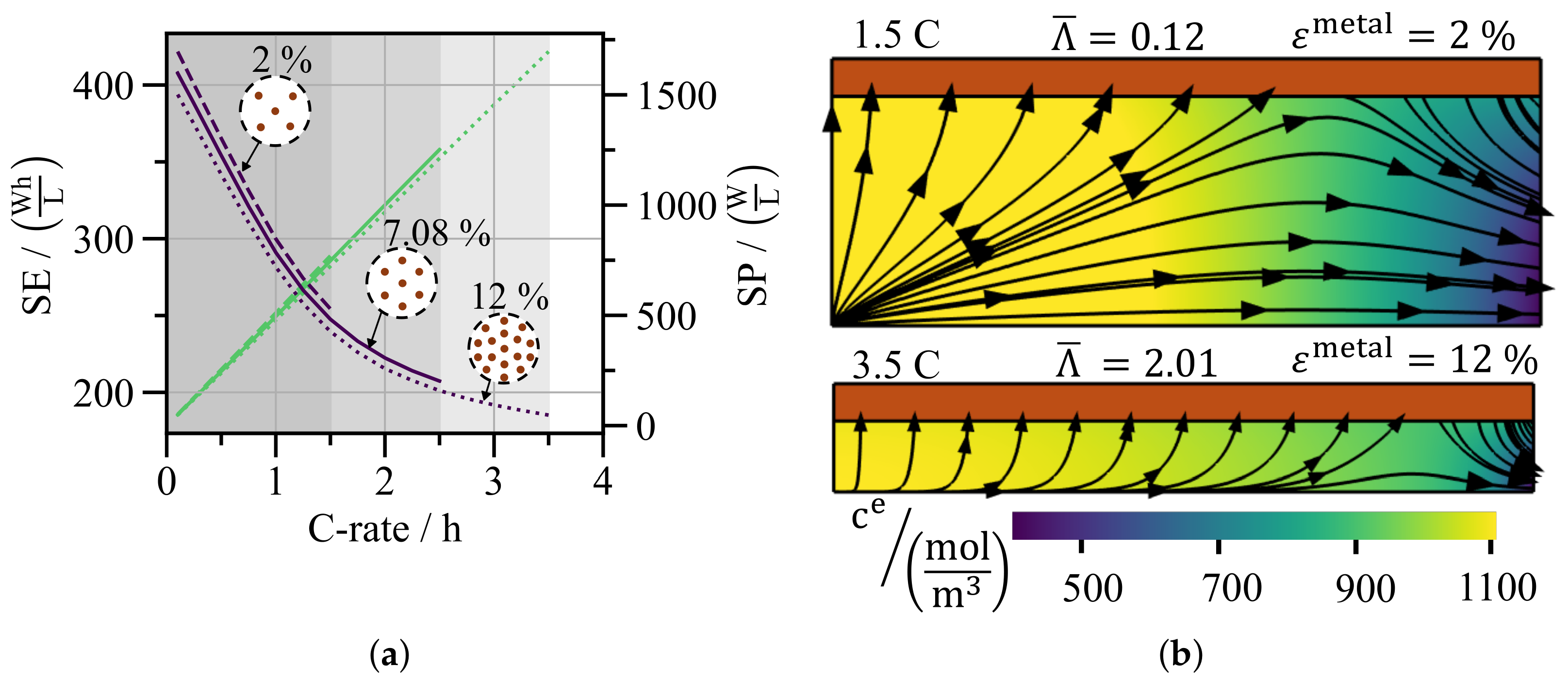
Metal fiber radius—Figure 11 evaluates the effect of the metal fiber radius by comparing the reference geometry with an electrode of identical thickness and fiber volume fraction , but a reduced metal fiber radius of . Since the fiber volume fraction and thus the active material volume are identical for both radii, the inactive volume penalty is the same and both electrodes reach the same volumetric energy density at low C-rates. As the pictograms in Figure 11a illustrate, reducing the metal fiber radius to at constant volume fraction increases the number of fibers per cross-section and therefore the specific metal fiber surface area . As shown by the 2D axis-symmetric domain in Figure 11b, a larger value of means less porous electrode volume per fiber surface, so most ions move along the fiber surface rather than through the porous electrode. This is confirmed quantitatively by , which corresponds to a surface flux share of . As shown in Figure 11a, the increased contribution of the high-mobility pathway extends the operating regime without electrolyte depletion from C to beyond 4 C. As a result, the electrode with thinner metal fibers reaches a volumetric power density up to .
Figure 11.
(a) (purple) and (green) as a function of the C-rate for the reference geometry (solid line) and for a decreased metal fiber radius (dashed line). The gray bands mark the operating regime without electrolyte depletion, defined by . (b) 2D axis-symmetric domain of the case with reduced metal fiber radius. The colormap shows the electrolyte concentration at the terminal time , with yellow and purple indicating high and low concentrations, respectively. The streamlines indicate the ion flux into and out of the EDL at the metal fiber surface.
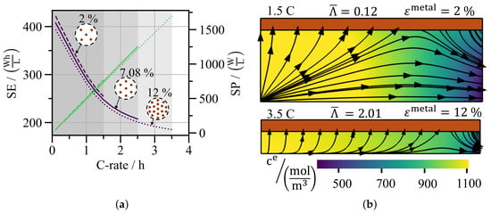
Volume fraction of metal fibers— Figure 12 analyzes the effect of varying metal fiber volume fraction at constant electrode thickness and metal fiber radius . Starting from the reference at , the volume fraction is reduced to and increased to .
Figure 12.
(a) (purple) and (green) as a function of the C-rate for the reference geometry (solid line) and for varying metal fiber volume fractions . The gray bands mark the operating regime without electrolyte depletion, defined by . (b) 2D axis-symmetric domain of the case with reduced (top) and increased (bottom) metal fiber volume fraction. The colormap shows the electrolyte concentration at the terminal time , with yellow and purple indicating high and low concentrations, respectively. The streamlines indicate the ion flux into and out of the EDL at the metal fiber surface.
Reducing the metal fiber volume fraction lowers the inactive volume penalty and increases the volumetric energy density at low C-rates. In contrast, increasing leads to a larger inactive volume penalty and a reduced at low C-rates.
As the pictograms in Figure 12a show, we vary the metal fiber volume fraction by removing or adding fibers of equal radius. Fewer fibers reduce the specific metal fiber surface area and weaken the contribution of the high-mobility pathway. More fibers have the opposite effect and strengthen the high-mobility pathway.
The streamlines in Figure 12b illustrate this directly. For , most ions choose the path through the porous electrode instead of the fiber surface. As a result, the surface flux share is only about (). For , the majority of ions follow the metal fiber surface, resulting in a surface flux share of ().
As shown in Figure 12a, the electrode with low metal fiber volume fraction operates without electrolyte depletion only up to C, which reduces the achievable volumetric power densities by approximately compared to the reference. The electrode with higher metal fiber volume fraction extends the operating regime to ~ C, raising by relative to the reference.
Unlike the variation of the metal fiber radius, varying the metal fiber volume fraction introduces a fundamental trade-off. A higher volume fraction extends the operating regime but increases the inactive volume penalty. This motivates the optimization of the fiber-fleece architecture, which is discussed in the following section.
3.3. Optimization
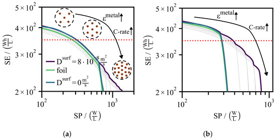
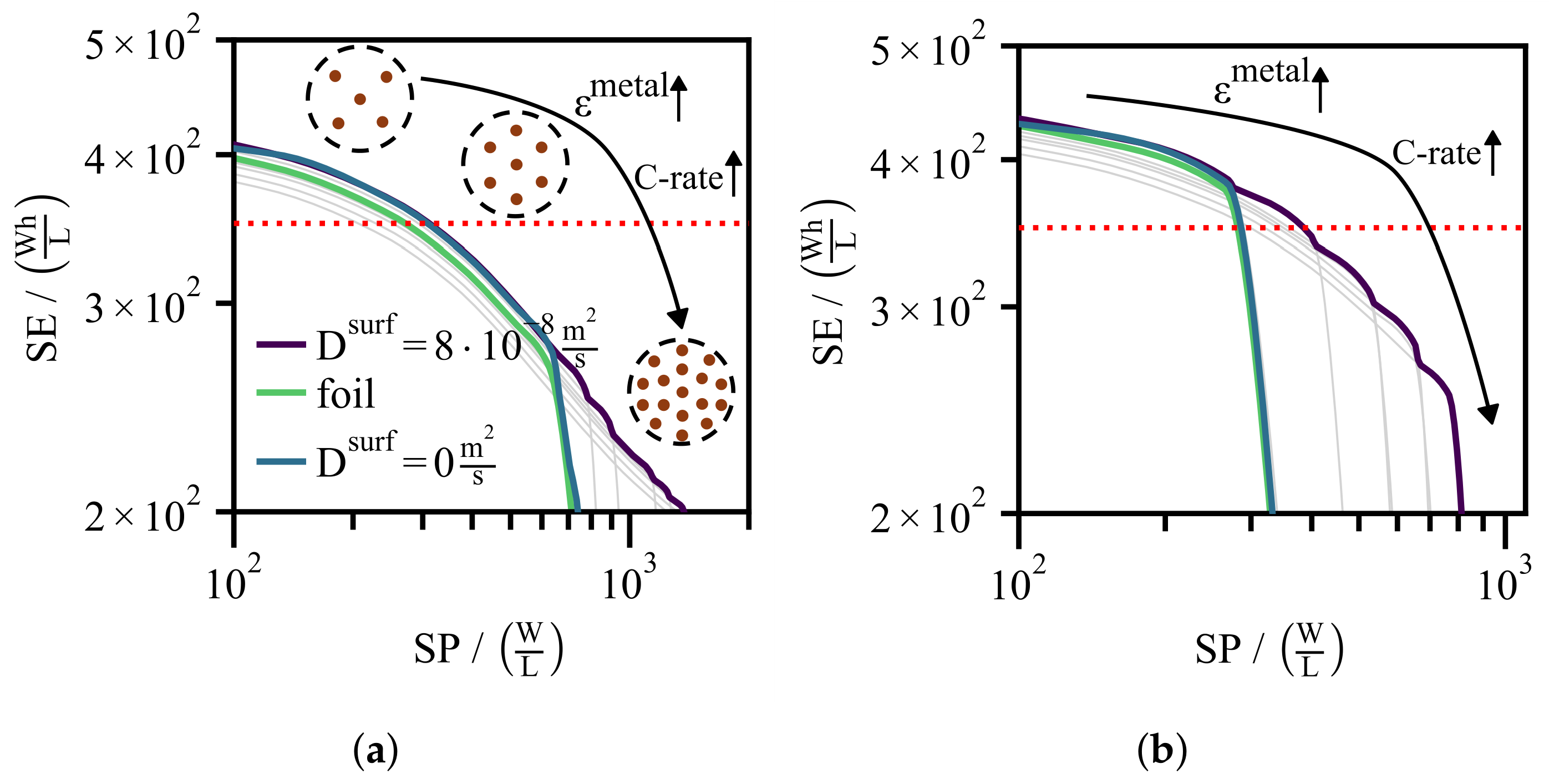
To emphasize the transport improvements provided by the high-mobility pathway in the EDL, the optimization is performed by varying the metal fiber volume fraction and the C-rate while keeping the electrode thickness constant at and the metal fiber radius at . The optimization objective is to maximize for a given target to derive design guidelines for the metal fiber architecture for different power density requirements. Although the fiber radius has a significant influence on and , it is treated as a design constraint rather than an optimization variable, since its variation does not introduce the inactive volume penalty trade-off that motivates the optimization. Figure 13 shows the optimized as a function of (purple Ragone curves). For comparison, the individual curves for different metal fiber volume fractions are shown in gray.
Figure 13.
Ragone plots for electrode thicknesses of (a) and (b) at fixed metal fiber radius . The gray Ragone curves correspond to different metal fiber volume fractions , with the curve that drops first corresponding to the smallest volume fraction. The optimized metal-fiber Ragone curve is shown as a purple solid line, the Ragone curve of the conventional foil-based electrode as a green solid line and the limit as a blue solid line. The red dotted line marks .
Electrodes with a planar current collector foil (green) serve as the benchmark. As confirmed in Section S8 of the Supplementary Materials, the limit corresponds to these foil-based electrodes, which can be described by the classical P2D model.
To distinguish between the contributions of the high-mobility pathway and the inactive volume penalty to the observed improvements, the limit with varying metal fiber volume fraction is included as an additional reference, where surface transport of the fiber-based electrodes is switched off (see Section S8 of the Supplementary Materials).
As shown in Figure 13a, for an electrode thickness of , low metal fiber volume fractions are optimal at lower power demands where the inactive volume penalty dominates. At higher power demands, a higher metal fiber volume fraction is required to increase the specific metal fiber surface area and enhance the high-mobility pathway in the EDL.
The power densities of all three scenarios are evaluated at (red dotted line) for a direct comparison in Table 4.
Table 4.
Volumetric power density at for the optimized fiber architecture (purple), the limit (blue), and the foil-based electrode (green).
Since the values of the fiber-based electrode and the limit are close, the improvement of the optimized Ragone curve over the foil-based electrode is driven primarily by the lower inactive volume penalty of the fiber architecture.
As shown in Figure 13b, the optimized Ragone curve for follows the same design guideline, with low metal fiber volume fractions being optimal at low power demands and high metal fiber volume fractions becoming optimal as the power demand increases. Since electrolyte diffusion limitation is more pronounced in thick electrodes, the high-mobility pathway contributes more strongly to the performance improvement. As confirmed by the limit, which lies close to the foil-based curve, the improvement can be attributed mainly to the high-mobility pathway rather than the inactive volume penalty. According to Table 4, the optimized fiber architecture improves over the foil-based electrode by approximately at .
4. Conclusions
This work builds on the experimental findings of Wang et al. [14], who demonstrated that a metal fiber fleece as a 3D current collector enhances the ion mobility by breaking ion-solvent complexes in the EDL. The resulting high-mobility pathway at the metal fiber surface provides an additional transport path, which improves the overall ion diffusivity with less pronounced electrolyte diffusion limitations.
Since the metal fiber fleece is electrochemically inactive, the central objective is to identify the optimal fiber architecture where the enhanced diffusivity overcompensates for the penalty from the inactive volume.
In the first part of this work, we propose a model approach for the high-mobility pathway in the EDL. For this purpose, the modified Poisson-Boltzmann model is reduced by treating the EDL as an effective boundary condition in the thin double layer limit. To prevent non-physical ion concentrations at high applied metal potentials , the modified Poisson-Boltzmann model captures steric effects which depend on the effective ion size a. The resulting quasi-equilibrium excess surface concentration , which depends on the effective ion size a, the potential and the bulk electrolyte concentration, is used to couple a surface transport equation with a bulk convection-diffusion model. Within this coupled model framework, the surface diffusivity and the effective ion size a are fitted against the microfluidic channel experiments.
In the second part, the fitted model framework is coupled to the P2D model to optimize the metal fiber-fleece architecture. The half-cell geometry is represented by a single cylindrical REV, comprising one metal fiber and the surrounding porous graphite electrode. Full-cell reconstruction with a virtual NMC111 cathode sets a realistic voltage window for evaluating volumetric energy density and power density .
Starting from a reference case with , , and , we vary the C-rate, electrode thickness, metal fiber radius and the metal fiber volume fraction to quantify their effect on volumetric energy density and power density . Thicker electrodes raise through a lower inactive volume penalty, but the electrolyte diffusion limitation becomes more pronounced and reduces the maximum C-rate before depletion. Metal fiber radius variation at constant volume fraction exhibits negligible effects on . Smaller radii increase the specific surface of the metal fibers , strengthening the high-mobility pathway and raising the maximum C-rate before electrolyte depletion. An increase in fiber volume fraction leads to lower (more inactive material) but larger maximum C-rates, resulting from the increased specific surface of the metal fibers.
Ragone-plot optimization at and with fixed metal fiber radius identifies design guidelines for the optimal metal fiber volume fraction across different power demands. At lower power, fewer metal fibers are preferable, as the inactive volume penalty dominates. At high power, the electrolyte diffusion limits performance. There, more metal fibers are required to increase and sustain the high-mobility pathway. In thicker electrodes, more pronounced electrolyte diffusion limitations lead to a larger improvement of the optimized fiber architecture over the foil-based design: at , the volumetric power density improves by approximately for and about for .
The model framework has three main limitations. First, the full-cell reconstruction is based on a virtual cathode. Since cathode polarization and transport limitations are neglected, the improvements of and represent an upper bound for a complete cell. Second, the potential of zero charge of copper in in EC/DMC is unknown and is set to vs. Li/Li+. The sensitivity analysis in Section S5 of the Supplementary Materials shows that and depend strongly on this value. Third, the P2D model is well established for lithium-ion batteries, but its coupling with the EDL surface transport model has not yet been validated experimentally for fiber-fleece electrodes. In addition, the REV assumes uniformly distributed, straight fibers.
To address these limitations, will be determined by differential capacitance measurements. The EDL framework will be coupled with the microstructure-resolved model of Latz and Zausch [23], which represents real porous electrode structures and fiber-fleece geometries, including curved and arbitrarily oriented fibers.
This allows direct experimental validation and the study of local current distributions and lithium plating during fast charging. Finally, the microfluidic channel experiment will be repeated with an aluminum surface to parameterize the cathode, enabling a full-cell simulation without virtual reconstruction.
Supplementary Materials
The following supporting information can be downloaded at: https://www.mdpi.com/article/10.3390/en19215177/s1, File S1: Supplementary Materials, containing Section S1: Experimental data of the microfluidic channel; Section S2: Mesh sensitivity analysis, microfluidic channel simulation; Section S3: Parameterization of the P2D model; Section S4: Mesh sensitivity analysis, half-cell simulation; Section S5: Sensitivity to uncertain model parameters; Section S6: Full-cell simulation; Section S7: Current inlet; Section S8: Limiting cases of the proposed battery model; Figure S1: Measured electrolyte concentration across the channel width for the remaining channel heights and applied potentials; Figure S2: Residual and parity plots for ; Figure S3: Residual and parity plots for ; Figure S4: Residual and parity plots for ; Figure S5: Interface displacement caused by the viscosity deviation between the two streams; Figure S6: Mesh sensitivity study and mesh for the microfluidic channel simulation; Figure S7: Basic functions of the electrolyte and the solid phase; Figure S8: Microscopic half-cell simulation setup and concentration distributions; Figure S9: Comparison between microscopic and P2D model at C; Figure S10: Mesh sensitivity study and mesh for the half-cell simulation; Figure S11: Simulation results for different effective ion sizes a; Figure S12: Volumetric energy and power densities for different effective ion sizes a; Figure S13: Simulation results for different potentials of zero charge; Figure S14: Full-cell simulation setup for the reference geometry; Figure S15: Volumetric energy and power density of the simulated and the reconstructed full cell; Figure S16: Full-cell voltage over time of the simulated and the reconstructed full cell; Figure S17: Simulation results for the two current inlet conditions; Figure S18: Comparison between the limiting case of the proposed model and the classical P2D model; Figure S19: Simulation results with and without surface diffusion; Table S1: RMSE for all channel heights, applied potentials and downstream positions; Table S2: Cell problems for the electrolyte and solid transport; Table S3: RMSE of the volumetric energy density for the alternative parameter sets; Table S4: Volumetric energy density of the simulated and the reconstructed full cell. References [23,24,25,26,36,42,45,46,47] are cited in the Supplementary Materials.
Author Contributions
Conceptualization, U.N. and J.P.S.; methodology, G.L. and Y.W.; software, G.L.; validation, G.L. and C.S.; investigation, G.L. and Y.W.; resources, Y.W.; writing—original draft preparation, G.L.; writing—review and editing, Y.W., C.S., U.N. and J.P.S.; visualization, G.L.; funding acquisition, U.N. and J.P.S. All authors have read and agreed to the published version of the manuscript.
Funding
This research was funded by the Deutsche Forschungsgemeinschaft (DFG, German Research Foundation) under grant number 507026050 and under Germany’s Excellence Strategy via the Excellence Cluster 3D Matter Made to Order (EXC-2082/1 – 390761711).
Data Availability Statement
The data that support the findings of this study are available from the corresponding author upon reasonable request.
Acknowledgments
The authors would like to acknowledge the generous and outstanding support of the Dieter Schwarz Foundation (DSS). They also gratefully acknowledge the excellent support of the Max Planck Society. During the preparation of this manuscript, the authors used Claude (Sonnet 4.5, Sonnet 4.6, Sonnet 5.5 and Opus 5.5) to assist with the formulation and wording of parts of the manuscript. The authors have reviewed and edited the output and take full responsibility for the content of this publication.
Conflicts of Interest
The authors declare no conflicts of interest.
Abbreviations
The following abbreviations are used in this manuscript:
| CBD | Carbon-binder domain |
| DMC | Dimethyl carbonate |
| EC | Ethylene carbonate |
| EDL | Electrical double layer |
| EIS | Electrochemical impedance spectroscopy |
| NMC | Nickel manganese cobalt (oxide) |
| OCV | Open-circuit voltage |
| P2D | Pseudo-two-dimensional |
| PB | Poisson-Boltzmann |
| PGSE-NMR | Pulsed gradient spin echo nuclear magnetic resonance |
| PNP | Poisson-Nernst-Planck |
| REV | Representative elementary volume |
| RMSE | Root mean square error |
| SEI | Solid electrolyte interphase |
Appendix A
The initial and boundary conditions of the P2D model for the half-cell setup are listed in Table A1.
Table A1.
Initial and boundary conditions of the P2D model for the half-cell.
The effective molar ion flux in the electrolyte is defined in Equation (18). The corresponding effective transport parameters are obtained from the asymptotic homogenization theory, as described in Section S3 of the Supplementary Materials.
Similarly, the effective electronic conductivity tensor is given by:
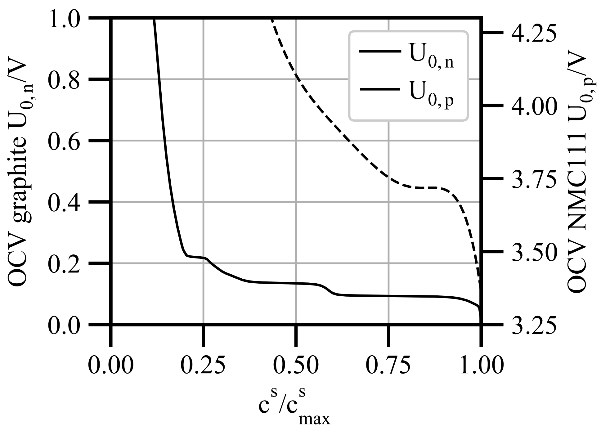
The remaining parameters for the half-cell model and the full-cell reconstruction are listed in Table A2. The geometric parameters are derived from the REV geometry, while the graphite electrode properties are taken from [30]. The parameters of the NMC111 cathode, used for the full-cell reconstruction, are obtained from Xu et al. [48].
Table A2.
Parameters of the half-cell simulation and the corresponding full-cell reconstruction. The electrolyte diffusivity and the ionic conductivity are listed in Table 2.
Both OCV profiles are displayed in Figure A1.
Figure A1.
Open-circuit voltage (OCV) of the graphite active material versus lithium (, solid black line) and of NMC111 vs lithium (, dashed black line).
References
- Masias, A.; Marcicki, J.; Paxton, W.A. Opportunities and challenges of lithium ion batteries in automotive applications. ACS Energy Lett. 2021, 6, 621–630. [Google Scholar] [CrossRef] [Scilit]
- Hesse, H.; Schimpe, M.; Kucevic, D.; Jossen, A. Lithium-Ion Battery Storage for the Grid—A Review of Stationary Battery Storage System Design Tailored for Applications in Modern Power Grids. Energies 2017, 10, 2107. [Google Scholar] [CrossRef] [Scilit]
- Phogat, P.; Dey, S.; Wan, M. Powering the sustainable future: A review of emerging battery technologies and their environmental impact. Rsc Sustain. 2025, 8, 3266–3306. [Google Scholar] [CrossRef] [Scilit]
- Zubi, G.; Dufo-López, R.; Carvalho, M.; Pasaoglu, G. The lithium-ion battery: State of the art and future perspectives. Renew. Sustain. Energy Rev. 2018, 89, 292–308. [Google Scholar] [CrossRef] [Scilit]
- Ngoy, K.R.; Lukong, V.T.; Yoro, K.O.; Makambo, J.B.; Chukwuati, N.C.; Ibegbulam, C.; Eterigho-Ikelegbe, O.; Ukoba, K.; Jen, T.-C. Lithium-ion batteries and the future of sustainable energy: A comprehensive review. Renew. Sustain. Energy Rev. 2025, 223, 115971. [Google Scholar] [CrossRef] [Scilit]
- Kuang, Y.; Chen, C.; Kirsch, D.; Hu, L. Thick electrode batteries: Principles, opportunities, and challenges. Adv. Energy Mater. 2019, 9, 1901457. [Google Scholar] [CrossRef] [Scilit]
- Heubner, C.; Nikolowski, K.; Reuber, S.; Schneider, M.; Wolter, M.; Michaelis, A. Recent insights into rate performance limitations of Li-ion batteries. Batter. Supercaps 2021, 4, 268–285. [Google Scholar] [CrossRef] [Scilit]
- Logan, E.R.; Dahn, J.R. Electrolyte design for fast-charging Li-ion batteries. Trends Chem. 2020, 2, 354–366. [Google Scholar] [CrossRef] [Scilit]
- Rakebrandt, J.-H.; Smyrek, P.; Zheng, Y.; Seifert, H.J.; Pfleging, W. Laser processing of thick Li(NiMnCo)O2 electrodes for lithium-ion batteries. In Proceedings of the Laser-Based Micro- and Nanoprocessing XI; Klotzbach, U., Washio, K., Kling, R., Eds.; SPIE: Bellingham, WA, USA, 2017; p. 100920M. [Google Scholar]
- Chen, K.-H.; Namkoong, M.J.; Goel, V.; Yang, C.; Kazemiabnavi, S.; Mortuza, S.M.; Kazyak, E.; Mazumder, J.; Thornton, K.; Sakamoto, J.; et al. Efficient fast-charging of lithium-ion batteries enabled by laser-patterned three-dimensional graphite anode architectures. J. Power Sources 2020, 471, 228475. [Google Scholar] [CrossRef] [Scilit]
- Sander, J.S.; Erb, R.M.; Li, L.; Gurijala, A.; Chiang, Y.-M. High-performance battery electrodes via magnetic templating. Nat. Energy 2016, 1, 16099. [Google Scholar] [CrossRef] [Scilit]
- Billaud, J.; Bouville, F.; Magrini, T.; Villevieille, C.; Studart, A.R. Magnetically aligned graphite electrodes for high-rate performance Li-ion batteries. Nat. Energy 2016, 1, 16097. [Google Scholar] [CrossRef] [Scilit]
- Zhang, H.; Yu, X.; Braun, P.V. Three-dimensional bicontinuous ultrafast-charge and -discharge bulk battery electrodes. Nat. Nanotechnol. 2011, 6, 277–281. [Google Scholar] [CrossRef] [Scilit] [PubMed]
- Wang, Y.; Aubermann, F.; Spatz, J.P. Enhanced ion mobility in Helmholtz layer enabling ultrathick electrodes. ACS Nano 2025, 19, 17917–17928. [Google Scholar] [CrossRef] [Scilit] [PubMed]
- Wu, Q.; McDowell, M.T.; Qi, Y. Effect of the electric double layer (EDL) in multicomponent electrolyte reduction and solid electrolyte interphase (SEI) formation in lithium batteries. J. Am. Chem. Soc. 2023, 145, 2473–2484. [Google Scholar] [CrossRef] [Scilit] [PubMed]
- Vlassiouk, I.; Smirnov, S.; Siwy, Z. Ionic selectivity of single nanochannels. Nano Lett. 2008, 8, 1978–1985. [Google Scholar] [CrossRef] [Scilit] [PubMed]
- Ma, L.; An, X.; Song, F.; Qiu, Y. Effective charged exterior surfaces for enhanced ionic diffusion through nanopores under salt gradients. J. Phys. Chem. Lett. 2022, 13, 5669–5676. [Google Scholar] [CrossRef] [Scilit] [PubMed]
- Bazant, M.Z.; Thornton, K.; Ajdari, A. Diffuse-charge dynamics in electrochemical systems. Phys. Rev. E 2004, 70, 021506. [Google Scholar] [CrossRef] [Scilit] [PubMed]
- Kilic, M.S.; Bazant, M.Z.; Ajdari, A. Steric effects in the dynamics of electrolytes at large applied voltages. I. Double-layer charging. Phys. Rev. E 2007, 75, 021502. [Google Scholar] [CrossRef] [Scilit] [PubMed]
- Yochelis, A.; Singh, M.B.; Visoly-Fisher, I. Coupling bulk and near-electrode interfacial nanostructuring in ionic liquids. Chem. Mater. 2015, 27, 4169–4179. [Google Scholar] [CrossRef] [Scilit]
- Kilic, M.S.; Bazant, M.Z.; Ajdari, A. Steric effects in the dynamics of electrolytes at large applied voltages. II. Modified Poisson-Nernst-Planck equations. Phys. Rev. E 2007, 75, 021503. [Google Scholar] [CrossRef] [Scilit] [PubMed]
- Bazant, M.Z.; Storey, B.D.; Kornyshev, A.A. Double layer in ionic liquids: Overscreening versus crowding. Phys. Rev. Lett. 2011, 106, 046102. [Google Scholar] [CrossRef] [Scilit] [PubMed]
- Latz, A.; Zausch, J. Thermodynamic consistent transport theory of Li-ion batteries. J. Power Sources 2011, 196, 3296–3302. [Google Scholar] [CrossRef] [Scilit]
- Less, G.B.; Seo, J.H.; Han, S.; Sastry, A.M.; Zausch, J.; Latz, A.; Schmidt, S.; Wieser, C.; Kehrwald, D.; Fell, S. Micro-scale modeling of Li-ion batteries: Parameterization and validation. J. Electrochem. Soc. 2012, 159, A697–A704. [Google Scholar] [CrossRef] [Scilit]
- Taralova, V.; Iliev, O.; Efendiev, Y. Derivation and numerical validation of a homogenized isothermal Li-ion battery model. J. Eng. Math. 2016, 101, 1–27. [Google Scholar] [CrossRef] [Scilit]
- Ciucci, F.; Lai, W. Derivation of micro/macro lithium battery models from homogenization. Transp. Porous Media 2011, 88, 249–270. [Google Scholar] [CrossRef] [Scilit]
- Doyle, M.; Fuller, T.F.; Newman, J. Modeling of galvanostatic charge and discharge of the lithium/polymer/insertion cell. J. Electrochem. Soc. 1993, 140, 1526–1533. [Google Scholar] [CrossRef] [Scilit]
- Traskunov, I.; Latz, A. New reduced-order lithium-ion battery model to account for the local fluctuations in the porous electrodes. Energy Technol. 2021, 9, 2000861. [Google Scholar] [CrossRef] [Scilit]
- Traskunov, I.; Latz, A. Localized fluctuations of electrochemical properties in porous electrodes of lithium-ion batteries: Beyond porous electrode theory. Electrochim. Acta 2021, 379, 138144. [Google Scholar] [CrossRef] [Scilit]
- Lombardo, G.; Wang, Y.; Stockinger, C.; Spatz, J.P.; Nieken, U. A particle-based model reduction for lithium-ion batteries. J. Electrochem. Soc. 2025, 172, 060512. [Google Scholar] [CrossRef] [Scilit]
- Fuller, T.F.; Doyle, M.; Newman, J. Relaxation phenomena in lithium-ion-insertion cells. J. Electrochem. Soc. 1994, 141, 982–990. [Google Scholar] [CrossRef] [Scilit]
- Newman, J.; Tiedemann, W. Porous-electrode theory with battery applications. Aiche J. 1975, 21, 25–41. [Google Scholar] [CrossRef] [Scilit]
- Chu, K.T.; Bazant, M.Z. Nonlinear electrochemical relaxation around conductors. Phys. Rev. E 2006, 74, 011501. [Google Scholar] [CrossRef] [Scilit] [PubMed]
- Chu, K.T.; Bazant, M.Z. Surface conservation laws at microscopically diffuse interfaces. arXiv 2007, arXiv:physics/0702042. [Google Scholar]
- Borukhov, I.; Andelman, D.; Orland, H. Steric effects in electrolytes: A modified Poisson-Boltzmann equation. Phys. Rev. Lett. 1997, 79, 435–438. [Google Scholar] [CrossRef] [Scilit]
- Lombardo, G.; Wang, Y.; Stockinger, C.; Spatz, J.P.; Nieken, U. A Particle-Based Model for Optimization of Lithium-Ion Battery Electrodes. J. Electrochem. Soc. 2026, 173, 200510. [Google Scholar] [CrossRef] [Scilit]
- Barthel, J.; Gores, H.J. Liquid Nonaqueous Electrolytes. In Handbook of Battery Materials; Besenhard, J.O., Ed.; Wiley-VCH: Weinheim, Germany, 1998; pp. 457–497. [Google Scholar]
- Yao, N.; Chen, X.; Shen, X.; Zhang, R.; Fu, Z.-H.; Ma, X.-X.; Zhang, X.-Q.; Li, B.-Q.; Zhang, Q. An atomic insight into the chemical origin and variation of the dielectric constant in liquid electrolytes. Angew. Chem. Int. Ed. 2021, 60, 21473–21478. [Google Scholar] [CrossRef] [Scilit] [PubMed]
- Karatrantos, A.V.; Khan, M.S.; Yan, C.; Dieden, R.; Urita, K.; Ohba, T.; Cai, Q. Ion transport in organic electrolyte solutions for lithium-ion batteries and beyond. J. Energy Power Technol. 2021, 3, 1–36. [Google Scholar] [CrossRef] [Scilit]
- Berhaut, C.L.; Lemordant, D.; Porion, P.; Timperman, L.; Schmidt, G.; Anouti, M. Ionic association analysis of LiTDI, LiFSI and LiPF6 in EC/DMC for better Li-ion battery performances. RSC Adv. 2019, 9, 4599–4608. [Google Scholar] [CrossRef] [Scilit] [PubMed]
- Ebner, M.; Chung, D.-W.; García, R.E.; Wood, V. Tortuosity anisotropy in lithium-ion battery electrodes. Adv. Energy Mater. 2014, 4, 1301278. [Google Scholar] [CrossRef] [Scilit]
- Fujieda, T.; Xia, Y.; Koike, S.; Shikano, M.; Sakai, T. Effect of acid on passivation of a copper electrode in LiCF3SO3/propylene carbonate in underpotential region. J. Power Sources 1999, 83, 186–192. [Google Scholar] [CrossRef] [Scilit]
- Ahmed, S.; Gejjiganahalli Ningappa, N.; Srivastava, M.; Bouguern, M.D.; M R, A.K.; Selva, T.M.G.; Dawkins, J.I.G.; Reddy, M.V.; Brassard, M.; Zaghib, K. Electrode balancing as a key factor in lithium-ion batteries: From fundamentals to ultrafast charging. J. Power Sources 2026, 667, 239188. [Google Scholar] [CrossRef] [Scilit]
- Alberto Ochoa-Tapia, J.; Del Antonio Rio, P.J.; Whitaker, S. Bulk and surface diffusion in porous media: An application of the surface-averaging theorem. Chem. Eng. Sci. 1993, 48, 2061–2082. [Google Scholar] [CrossRef] [Scilit]
- Bensoussan, A.; Lions, J.-L.; Papanicolaou, G. Asymptotic Analysis for Periodic Structures; Studies in Mathematics and Its Applications; North-Holland: Amsterdam, The Netherlands, 1978; Volume 5. [Google Scholar]
- Allaire, G.; Raphael, A.-L. Homogenization of a convection–diffusion model with reaction in a porous medium. Comptes Rendus Mathématique 2007, 344, 523–528. [Google Scholar] [CrossRef] [Scilit]
- Tang, W.; Zhao, S.; Huang, J. Origin of solvent dependency of the potential of zero charge. JACS Au 2023, 3, 3381. [Google Scholar] [CrossRef] [Scilit] [PubMed]
- Xu, M.; Reichman, B.; Wang, X. Modeling the effect of electrode thickness on the performance of lithium-ion batteries with experimental validation. Energy 2019, 186, 115864. [Google Scholar] [CrossRef] [Scilit]

Disclaimer/Publisher’s Note: The statements, opinions and data contained in all publications are solely those of the individual author(s) and contributor(s) and not of MDPI and/or the editor(s). MDPI and/or the editor(s) disclaim responsibility for any injury to people or property resulting from any ideas, methods, instructions or products referred to in the content. |
© 2026 by the authors. Licensee MDPI, Basel, Switzerland. This article is an open access article distributed under the terms and conditions of the Creative Commons Attribution (CC BY) license.