Passive–Active Co-Design for Robust LCL-Filtered Grid-Connected Photovoltaic Inverters

Abstract

Efficient operation of LCL-filtered grid-connected photovoltaic inverters under uncertain grid conditions requires coordinated treatment of passive-filter and current-controller interactions. This study addresses the interaction mechanism between passive LCL network parameters and active controller parameters through a systematic simultaneous passive–active co-design framework for a 10 kW inverter. A controlled five-strategy M1–M5 comparison separates conventional, control-only, passive-network-only, sequential, and simultaneous designs under a common plant, delay, modulation, switching, FFT, and uncertainty-validation protocol. Multi-objective search is supported by fast physical indicators, while leakage-free Gaussian process regression is used only as a candidate-screening accelerator before direct switching verification. The selected M5 design achieves a switching-model current total harmonic distortion of 0.8004%, passive damping loss of 8.236 W, and nominal phase and gain margins of 59.13° and 8.13 dB, respectively. Across 1000 shared Monte Carlo samples, its strict acceptance ratio is 98.3%, with zero true discrete-pole instability; rejected samples are conservative all-crossover margin anomalies. These simulation-based results indicate that M5 provides a balanced engineering compromise among harmonic performance, damping loss, dynamic response, and robustness rather than a design that dominates every individual metric. Gaussian process regression reduces screening cost but neither defines the objective nor replaces high-fidelity validation. Hardware-in-the-loop and experimental validation remain future work.

1. Introduction

1.1. Challenges of LCL-Filtered Grid-Connected Photovoltaic Inverters

Grid-connected photovoltaic (PV) inverters increasingly operate as actively controlled grid interfaces rather than passive power-injection units. Their current quality, dynamic tracking, and stability depend on the interaction among the converter, the grid-interface filter, digital control, and a grid impedance that may vary over operating conditions. LCL filters are attractive because they provide stronger switching-frequency attenuation than a single inductor, but their resonance introduces an additional stability problem [1,2,3,4,5,6].

For a practical PV inverter, the interface design must therefore balance power quality, passive loss, magnetic utilization, controller bandwidth, digital delay, and robustness. Treating any one of these aspects in isolation can transfer the burden to another part of the system rather than improve the complete converter.

1.2. Coupled LCL Passive-Network and Controller Design

The design contains two coupled spaces. The passive topology is described by the inverter-side inductance L₁, grid-side inductance L₂, filter capacitance C_f, and series damping resistor R_d. In this study, passive topology design refers to the parameterized design of the passive network within the fixed LCL configuration through L₁, L₂, C_f, and R_d, rather than structural topology synthesis among different filter configurations. Accordingly, the terms passive-network-only and passive–active co-design denote optimization of the passive-network parameters and their coordination with the controller parameters within the fixed LCL configuration. The active controller is described here by the quasi-proportional-resonant gains K_p and K_r and the capacitor current feedback gain K_a. The passive variables determine resonance location, ripple attenuation, reactive current, and damping loss, while the controller reshapes the same resonance and determines tracking and delay sensitivity [7,8,9,10,11,12,13]. Grid impedance further changes the effective plant seen by the controller [14,15,16,17].

This coupling means that a topology judged feasible using conventional component rules may still produce weak controlled margins, whereas a controller tuned for one topology may become unnecessarily conservative or ineffective after the filter parameters change. A fair method comparison must therefore keep the plant model, passive-damping representation, modulation limit, delay model, margin routine, switching model, and FFT window identical.

1.3. Limitations of Existing Design Sequences

Existing studies have addressed different parts of the LCL-filtered inverter design problem separately. Passive-network studies include LCL parameter design and optimization [18,19,20], passive damping [21,22], and magnetic integration [23]. Controller-oriented stabilization includes PLL and phase-compensation methods [24,25,26,27], PR-based control [28,29], capacitor current and wide-band active damping [30,31,32], hybrid damping [33,34,35], delay compensation and direct grid-current control [36,37], and active damping/current-controller co-design [38].

Reference [38] co-designs the active damping loop and grid-current controller for an LCL-filtered inverter. The present work addresses a different methodological question: the passive-network parameters (L₁, L₂, C_f, and R_d) and controller parameters (K_p, K_r, and K_a) are coordinated within one fixed-LCL design space, and the controlled M1–M5 framework separates controller-only, passive-network-only, sequential, and simultaneous effects. Direct switching verification and a shared-sample uncertainty audit are then applied to the selected designs. The contribution is therefore the coupled formulation and controlled comparative evidence, rather than a claim that this study introduces a new optimization algorithm or the general concept of controller co-design.

Robustness studies address system-level grid-impedance allocation [39], parametric uncertainty [40,41], weak-grid multiresonance and multi-bus interactions [42,43], and passivity- or impedance-based stabilization [44,45]. Sequential control formulations have also been investigated [46]; in the design sequence considered here, fixing the first-stage topology restricts the controller search space of the second stage.

Harmonic assessment is considered in [47]. Surrogate-assisted optimization can reduce expensive model evaluations [48,49,50,51], while NSGA-II provides the multiobjective Pareto-search engine [52]. Interconnection and harmonic requirements are documented in IEEE Std 1547 and IEEE Std 519 [53,54].

Despite these advances, four gaps remain relevant to the present study. First, controller-oriented tuning cannot directly redesign the passive resonance and loss mechanisms. Second, passive-filter optimization alone does not explicitly coordinate the resulting plant with controller compensation requirements. Third, sequential topology-then-controller design remains order dependent because the first-stage decision constrains the second-stage search space. Fourth, high-fidelity switching evaluation of a large candidate archive remains computationally expensive, which motivates surrogate screening provided that final claims are verified by direct switching simulation. These complementary gaps motivate the controlled M1–M5 comparison, which isolates controller-only, passive-network-only, sequential, and simultaneous design effects under one common validation protocol.

Therefore, a systematic framework that simultaneously considers passive LCL topology and active controller parameters, while combining surrogate-assisted screening with high-fidelity switching verification, is required to achieve a balanced trade-off among harmonic performance, damping loss, dynamic response, and robustness.

1.4. Contributions and Paper Organization

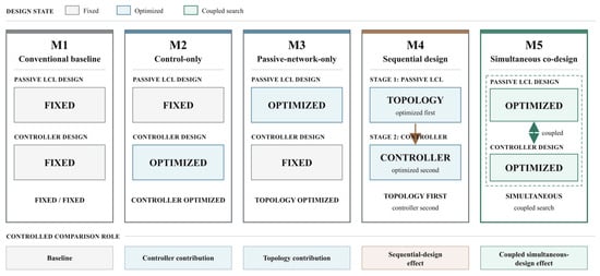
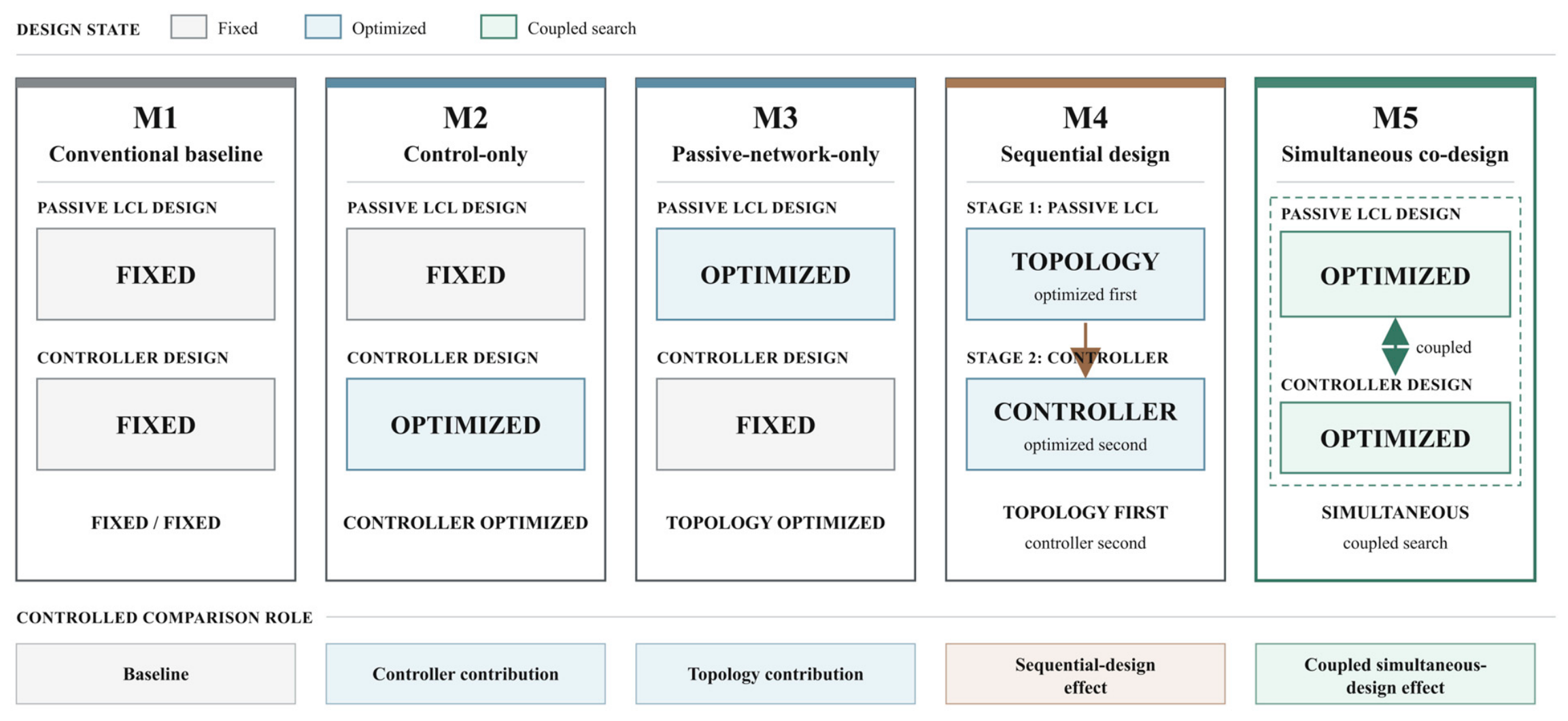
This paper establishes a controlled five-strategy comparative framework (M1–M5) to quantitatively decouple the individual and coupled contributions of passive filter topology and active controller design. M1 provides the conventional baseline, M2 isolates the controller-only contribution, M3 isolates the passive-network-only contribution with the M1 controller fixed, M4 exposes the limitation of sequential optimization, and M5 quantifies the simultaneous coupling effect.

A simultaneous LCL-parameter and controller co-design formulation is developed to explicitly coordinate passive resonance shaping and active damping compensation within a unified design space.

The key contribution is not the increase in optimization dimensions, but the explicit formulation of the coupled interaction between passive-network characteristics and controller compensation requirements. By considering both effects within a unified design space, the proposed framework reveals the trade-off relationships that cannot be captured by independent optimization sequences.

A leakage-free GPR-assisted screening strategy is introduced to reduce the computational burden of high-fidelity switching evaluations. The surrogate model serves only as a candidate screening tool and does not replace switching verification.

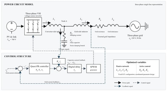
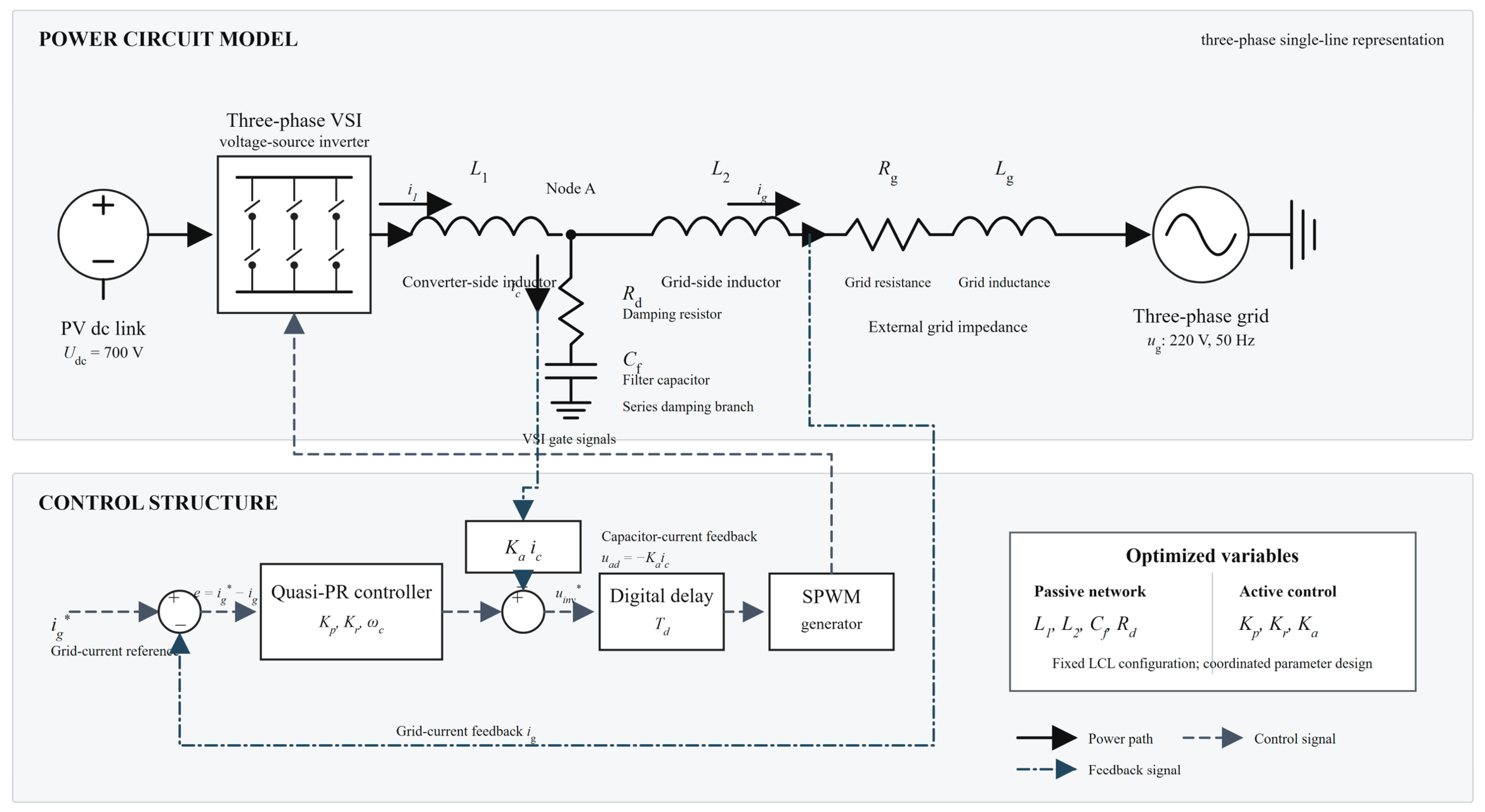
A unified uncertainty validation framework is conducted using identical Monte Carlo samples and criteria for all design strategies. An all-crossover and discrete-pole audit distinguishes strict margin rejection from true pole instability. Figure 1 summarizes the system configuration and control structure used for the comparative analysis.

Figure 1. System configuration of the grid-connected PV inverter with LCL filter and active damping control, including the power-stage topology, grid impedance, and capacitor current feedback control loop.

Unlike conventional approaches that optimize passive filtering and controller tuning as separate design stages, this study formulates the LCL-filtered inverter as a coupled passive-active system. In this formulation, passive-network parameters modify the resonance characteristics and damping requirements observed by the controller, while controller parameters influence the feasible passive-network compromise through active damping capability and dynamic constraints. Therefore, the design problem is treated as a coordinated interaction rather than an independent parameter optimization problem.

2. System Description and Unified Model

2.1. System Configuration

The study considers the grid-side conversion stage of a 10 kW three-phase grid-connected photovoltaic inverter. An ideal 700 V DC source represents a regulated DC link maintained by the upstream PV-side conversion stage, thereby isolating the passive-active interaction of the grid-current loop. PV-array dynamics, irradiance and temperature variation, maximum-power-point tracking, and DC-link outer-loop dynamics are outside the present scope. Accordingly, the photovoltaic designation identifies the intended application, whereas the technical claims are limited to the grid-side VSI, LCL filter, current controller, and grid-impedance interaction. The inverter is connected to a 220 V RMS phase-voltage, 50 Hz grid through an LCL filter and external grid impedance. The common implementation parameters are listed in Table 1.

Table 1. System and controller implementation parameters.

Parameter	Symbol	Value	Unit
Rated active power	Pn	10,000	W
DC-link voltage	Udc	700	V
Grid phase voltage	Ug,rms	220	V RMS
Grid frequency	fg	50	Hz
Switching frequency	fsw	10,000	Hz
Control sampling frequency	fs	10,000	Hz
Switching-model step	Ts,sim	1	μs
Nominal grid resistance	Rg	0.10	Ω
Nominal grid inductance	Lg	0.50	mH
Inverter-side parasitic resistance	R1	0.08	Ω
Grid-side parasitic resistance	R2	0.05	Ω
Nominal digital delay	Td	1.5	Ts
SPWM modulation limit	mlim	0.98	p.u.
Control sampling period	Ts	100	μs
PR fundamental angular frequency	w0	314.159	rad/s
PR resonant bandwidth	wc	31.416	rad/s
Proportional gain	Kp	Method-specific	V/A
Resonant gain	Kr	Method-specific	V/A
Active damping gain	Ka	Method-specific	V/A

Note: Values already reported as system parameters are not duplicated. The controller gains follow the direct physical-unit convention used in the simulation model, and method-specific K_p, K_r, and K_a values are reported in the later method-comparison table. The frozen M1 benchmark uses K_p = 9.6936982919 V/A, K_r = 31.0296969696 V/A, K_a = 0 V/A, and the archived resonant-bandwidth parameter w_c = 12.8463151978 rad/s. The common w_c = 31.416 rad/s value in Table 1 applies to the unified controller description unless a method-specific archived configuration is explicitly retained. Preserving the stated M1 configuration reproduces the formally recorded conventional-baseline switching result; the other methods use their finalized controller configurations reported in that comparison.

2.2. Unified LCL Plant and Current Controller

For one stationary-frame axis, the state vector is x = [i₁, u_c, i_g]^T and the capacitor current direction is i_c = i₁ − i_g. The damping resistor is represented consistently as a series element in the capacitor branch. Equations (1)–(3) define the plant, Equation (4) gives the resonance frequency including the external grid inductance when grid-strength variation is studied, and Equation (5) defines the quasi-PR controller.

$$L_1{\displaystyle \frac{\mathrm{d}{i}_1}{\mathrm{d}t}} = u_i - u_c - R_1{i}_1 - R_d\left(i_1 - i_g\right)$$

(1)

$$C_f{\displaystyle \frac{\mathrm{d}{u}_c}{\mathrm{d}t}} = i_1 - i_g$$

(2)

$$\left(L_2 + L_g\right){\displaystyle \frac{\mathrm{d}{i}_g}{\mathrm{d}t}} = u_c - u_g - \left(R_2+R_g\right)i_g + R_d\left(i_1 - i_g\right)$$

(3)

$$f_r = {\displaystyle \frac{1}{2\pi }}\sqrt{{\displaystyle \frac{L_1 + L_2 + L_g}{L_1\left(L_2 + L_g\right)C_f}}}$$

(4)

$$G_c\left(s\right) = K_p+{\displaystyle \frac{2K_r{\omega }_{c}s}{s^2 + 2{\omega }_{c}s + {\omega }_0^2}}$$

(5)

Capacitor current feedback is applied as u_ad = −K_a i_c, and grid-voltage feedforward is added to the inverter voltage command. The stationary-frame current error is expressed in amperes and the controller output is a phase-voltage command in volts; consequently, K_p, K_r, and K_a are reported in V/A under the model’s direct physical-unit convention, without an additional per-unit normalization. The controller gains are reported according to the implementation convention used in the simulation model. K_a supplies active damping through the measured capacitor current, but its useful range is constrained by digital-delay phase lag and the SPWM modulation limit. The same unified plant is used for controller tuning, optimization, frequency-domain analysis, the fast discrete model, and the switching-function model.

The unified quasi-PR controller description uses w₀ = 2π(50) = 314.159 rad/s and w_c = 2π(5) = 31.416 rad/s unless a method-specific archived controller configuration is explicitly retained for baseline reproduction. In particular, the frozen M1 benchmark uses w_c = 12.8463151978 rad/s together with the K_p, K_r, and K_a values stated in the note to Table 1. For both stationary-frame axes, the resonant state-space realization is discretized at Ts = 100 μs by the ordinary bilinear transform (Tustin method), without frequency prewarping. The proportional term Kp remains the direct feedthrough term.

For implementation, the resonant state is x_r = [x_r1, x_r2]^T with A_r = [0, 1; −ω₀², −2 ω_c], B_r = [0; 1], C_r = [0, 2 K_r ω_c], and D_r = K_p. Ordinary Tustin discretization gives A_d = (I − T_s A_r/2)⁽⁻¹⁾(I + T_s A_r/2), B_d = (I − T_s A_r/2)⁽⁻¹⁾ T_s B_r, C_d = C_r (I − T_s A_r/2)⁽⁻¹⁾, and D_d = D_r + C_r (I − T_s A_r/2)⁽⁻¹⁾ _Ts B_r/2. No prewarping at ω₀ or any other frequency is used.

For the frozen M1 implementation (T_s = 100 microseconds and archived w_c = 12.8463151978 rad/s), the numerical matrices are _Ad = [0.999507274326, 9.98470969883 × 10⁻⁵; −9.85451347872, 0.996941939767], B_d = [4.99235484942 × 10⁻⁹; 9.98470969884 × 10⁻⁵], C_d = [−3928.17923802, 796.015539911], and D_d = 9.73349906891. These coefficients are reported at reproduction precision and are not rounded values used internally by the evaluator.

For stability-margin evaluation, the loop is broken at the negative grid-current feedback path, for which e = i_ref − i_g. The return ratio contains the zero-order-held unified plant, the quasi-PR controller, the inner capacitor current active damping feedback, and the specified digital command delay T_d. The grid-voltage feedforward path is excluded because it is an additive exogenous path and does not close the grid-current feedback loop. No additional unreported PWM or sampling delay is added to T_d.

2.3. Digital Implementation and Common Validation Protocol

The frequency-domain model represents the specified command delay exactly by exp(−jwT_d). Integer delays in the rapid discrete model are exact shift registers. For a noninteger delay, the automatic path first tests a second-order Thiran all-pass realization. The candidate is accepted only when its maximum absolute phase error is no greater than 2 degrees and its maximum absolute magnitude error is no greater than 0.2 dB over 0−3 kHz on a 400-point validation grid. For 1.5 T_s, the second-order Thiran response has a 6.348-degree maximum phase error and therefore activates the fallback.

The fallback tests real-coefficient band-limited least-squares FIR orders 2−14 using an 800-point design grid and retains the first order that satisfies both limits. The selected 1.5 T_s implementation is order 8, with maximum errors of 1.430 degrees and 0.164 dB over the validation band. The switching model instead uses the exact simulation-step delay buffer described in Section 3.5. Because the inverter uses triangular-carrier SPWM, the available phase-voltage peak is m_limU_dc/2; the SVPWM value U_dc/sqrt(3) is not used. Phase and gain margins are obtained from all crossover points and are cross-checked with MATLAB all-margin when available. All numerical analyses and switching-function simulations reported in this study were performed using MATLAB/Simulink R2023b.

The high-fidelity implementation is a deterministic three-phase switching-function-based time-domain evaluator with a 1 μs fixed step. Final harmonic values are calculated from the last ten complete 50 Hz periods after steady state, with the DC component removed and harmonics from the second to the fiftieth order included. Components around the switching frequency are reported separately from THD_sw.

2.4. Conventional M1 Design Procedure

The conventional passive network is fixed before controller retuning. At 10 kW and 220 V RMS phase voltage, the rated phase current is I_rms = P_n/(3U_g,rms) = 15.1515 A and I_peak = sqrt(2)I_rms = 21.4275 A. The allowable inverter-side peak-to-peak ripple is 0.30I_peak = 6.4282 A. Using the conservative SPWM estimate Delta i_1,pp = U_dc/(6L₁f_sw), L₁ = 1.9 mH gives 6.1404 A, or 28.66% of rated peak current. The adopted inductance split L₂/L₁ = 0.4 gives L₂ = 0.76 mH.

The capacitor value C_f = 5 microfarads gives Q_c = 3w_gC_fU_g,rms² = 228.08 var, equal to 2.28% of rated power. With the external grid inductance excluded from the conventional component check, f_r = (1/(2pi))sqrt((L₁ + L₂)/(L₁L₂C_f)) = 3054.87 Hz, which satisfies 10f_g ≤ f_r ≤ 0.5f_sw. The fundamental inductor-voltage-drop ratio is 5.76%. The empirical series-damping relation R_d = 1/(3(2pi f_r)C_f) gives 3.4733 ohms; the implemented value is 3.47 ohms. Thus, the conventional set satisfies the 30% ripple, 5% capacitor-reactive-power, resonance-window, and 10% voltage-drop checks before closed-loop tuning.

The conventional controller retains K_a = 0. Its reproducible gain tuning first scans f_c = 400:25:800 Hz and 35 logarithmically spaced K_r values from 15 to 150, with K_p = (L₁ + L₂)2pi f_c. Nominally stable points must satisfy PM ≥ 45 degrees, GM ≥ 6 dB, and modulation ≤ 0.98. The five leading coarse points are refined over f_c +/− 50 Hz in 5 Hz increments and K_r from 0.70 to 1.30 times each seed using 21 logarithmic points. The top three nominally feasible points are then switching-verified, and the first normal steady-state case is frozen as M1. This procedure yields K_p = 9.6936982919 V/A and K_r = 31.0296969696 V/A; the archived M1 resonant-bandwidth configuration is retained as specified in Section 2.2.

3. Proposed Passive–Active Co-Design Framework

3.1. Problem Formulation

The simultaneous decision vector is x = [L₁, L₂, C_f, R_d, K_p, K_r, K_a], where K_a is implemented in the project as K_ad. The fast-search objective vector contains THD_est, passive damping-loss estimate, total inductance L_sum = L₁ + L₂, current-step ITAE, negative worst phase margin, and negative worst gain margin. THD_est is a physics-based screening indicator and is never substituted for the final switching-model THD_sw.

The optimization is constrained by conventional LCL feasibility, nominal closed-loop stability, all-crossover margins, and SPWM modulation. Robust candidate refinement then evaluates the common grid-resistance, grid-inductance, and delay domain before switching verification. Infeasible candidates receive finite penalties rather than missing objective values.

During rapid candidate evaluation, the worst-margin objectives are calculated at L_g = [0.1, 0.5, 1.0, 2.0, 3.0] mH and T_d = [1.0, 1.5, 2.0] T_s with R_g fixed at its nominal value of 0.10 ohm, giving 15 operating points. The final robustness audit is broader: it uses the full Cartesian product of the same five L_g values, R_g = [0.05, 0.10, 0.20, 0.30, 0.40] ohm, and the three delay values, giving 75 operating points. The rapid-search objective and final reported audit are therefore not treated as equivalent.

3.2. Comparative Design Strategies for Passive–Active Co-Design Evaluation

M1–M5 are defined by which variable groups are allowed to change. M3 fixes the complete M1 controller, including K_a = 0, while optimizing only the four LCL parameters. M4 first selects a topology with the M1 controller fixed and then tunes the controller with that topology fixed. Consequently, M4 is a sequential baseline and is not equivalent to M5, which searches all seven variables simultaneously. Figure 2 provides a visual comparison of the five controlled design strategies, while Table 2 gives their corresponding optimization variables, fixed quantities, bounds, and engineering constraints.

Figure 2. Comparison of five controlled design strategies for passive–active co-design evaluation. Gray, blue, and green blocks denote fixed, independently optimized, and coupled-search de-sign states, respectively; the dashed outline in M5 groups the jointly optimized passive-network and controller variables.

Table 2. Optimization variables, bounds, and engineering constraints.

Category	Method or Item	Variables or Range	Fixed Variables or Criterion
Strategy	M1 conventional	None	Conventional topology and fixed M1 controller
Strategy	M2 control-only	Kp, Kr, Ka	L1, L2, Cf, and Rd fixed to M1
Strategy	M3 passive-network-only	L1, L2, Cf, Rd	Kp, Kr, and Ka fixed to M1
Strategy	M4 sequential	Topology, then controller	Only one variable group changes in each stage
Strategy	M5 simultaneous	All seven variables	One coupled Pareto search; no M2–M4 initialization
Search bound	L1	0.5–3.0 mH	Logarithmic encoding
Search bound	L2	0.2–2.0 mH	Logarithmic encoding
Search bound	Cf	2–15 μF	Logarithmic encoding
Search bound	Rd	0–8 Ω	Linear encoding
Search bound	Kp	2.908–29.081	Linear encoding; 0.3–3 times M1
Search bound	Kr	6.206–155.148	Logarithmic encoding; 0.2–5 times M1
Search bound	Ka	0–10	Linear encoding
Constraint	Resonance frequency	500–5000 Hz	10fg ≤ fr ≤ 0.5fsw
Constraint	Capacitor reactive power	≤5% of rated power	Engineering feasibility
Constraint	Inductor voltage drop	≤10% of phase voltage	Engineering feasibility
Constraint	Inverter-side ripple	≤30% of rated peak current	Engineering feasibility
Constraint	Nominal PM and GM	≥45° and ≥6 dB	All-crossover calculation
Constraint	SPWM modulation	≤0.98; no saturation	Available phase peak = 0.98Udc/2
Selection filter	M5 total inductance	≤3.5 mH	Switching-aware candidate refinement
Selection filter	M5 ITAE	≤3 × M1 ITAE	Avoid severe dynamic degradation

Note: M5 bounds and encoding are taken from the simultaneous-search configuration. The L_sum and ITAE rows are switching-aware candidate-selection filters applied after the Pareto search.

3.3. Simultaneous Co-Design Framework

NSGA-II is adopted as the search engine for exploring the coupled design space, using a population of 120, 100 generations, crossover probability 0.90, mutation probability 1/7, and random seed 20260721. L₁, L₂, C_f, and K_r use logarithmic encoding to limit scale imbalance. The Pareto archive is generated independently of M2−M4; those methods are used only for post-selection comparison. The methodological contribution lies in formulating and validating the coupled interaction between passive-network design and controller compensation rather than introducing a new optimization algorithm.

Optimizer repeatability was evaluated through 20 independent runs using different recorded seeds while retaining the same population size (120), generation count (100), crossover probability (0.90), mutation probability (1/7), objectives, bounds, and constraints. A common normalized empirical nondominated union containing 2052 points was used as the reference front. Across the 20 runs, the approximate hypervolume was 0.5213 +/− 0.0351 (range 0.4628–0.5888), and IGD was 0.1614 +/− 0.0060 (range 0.1535–0.1754). Every run produced 117 feasible nondominated points with a final feasible ratio of 1.0. Nineteen of the 20 independently selected fast-stage compromise points lay within 1% of at least one variable bound, indicating that stochastic dispersion and boundary sensitivity remain relevant. These repeats assess search reproducibility only; they do not replace or reselect the frozen switching-verified Candidate 15.

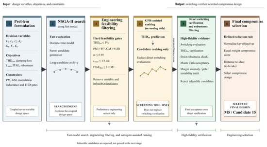
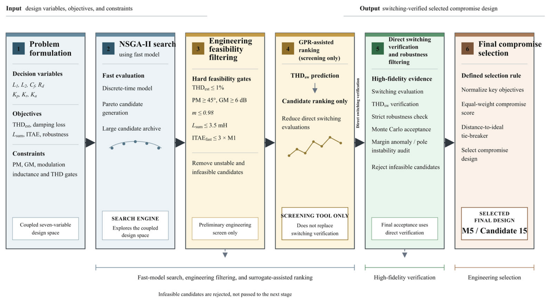
Candidates are first filtered by engineering feasibility and nominal stability. The compromise selection jointly considers THD_est, passive damping loss, total inductance, ITAE, and robust PM/GM rather than selecting a maximum-margin or minimum-THD point. An initial fast-model knee candidate that did not reach switching-model steady state was rejected. The final M5 result is therefore drawn from the switching-verified, robust candidate set without changing the simultaneous optimization framework. Figure 3 summarizes the staged candidate-generation and verification workflow, in which NSGA-II search, engineering screening, GPR-assisted ranking, and switching-domain robustness verification are combined to identify the final selected compromise design.

Figure 3. Workflow of simultaneous co-design, surrogate-assisted candidate ranking, and switching-verified final compromise selection. Blue, yellow, green, and brown blocks denote problem/search, engineering screening/ranking, direct verification, and final selection stages, respectively; arrows indicate the direction of candidate flow.

Final Compromise Selection Strategy

Step 1 generates the simultaneous M5 Pareto archive from the seven-variable search. Step 2 applies the predefined engineering and hard feasibility gates: valid LCL constraints, closed-loop stability, nominal PM ≥ 45°, nominal GM ≥ 6 dB, maximum modulation index ≤ 0.98, L_sum ≤ 3.5 mH, and ITAE_fast ≤ 3 × M1 ITAE. No M2–M4 result initializes or modifies this archive.

Step 3 sends representative feasible candidates to the common switching-function model. A candidate is rejected if it does not reach steady state, has a nonzero saturation duration, or does not provide a valid FFT window; THD_est is never substituted for THD_sw. The subsequent benchmark-aware and robust gates require THD_sw ≤ 1%, passive damping loss below M1, stable poles throughout the common grid-delay scan, worst PM ≥ 45°, and worst GM ≥ 6 dB.

The gate values serve distinct engineering and screening purposes. PM ≥ 45 degrees and GM ≥ 6 dB are conventional robustness targets applied consistently to every method, rather than statutory limits. The modulation limit of 0.98 preserves a 2% command headroom below the linear SPWM boundary defined by U_dc/2. The Lsum limit of 3.5 mH is 31.6% above the conventional M1 value of 2.66 mH and prevents the search from obtaining attenuation primarily through unrestricted magnetic oversizing. The ITAE_fast limit of three times the M1 value rejects severe dynamic degradation while retaining a broad Pareto pool. The 1% THD_sw threshold is an internal switching-candidate screen selected to retain designs close to the conventional benchmark; it is not presented as an IEEE 519 compliance limit. Requiring passive damping loss below M1 ensures that a retained co-design does not obtain its performance solely through increased resistive dissipation.

Step 4 normalizes the verified THD_sw, passive damping loss, L_sum, ITAE_fast, and robustness quantities over the eligible pool. Robustness is the mean benefit obtained from the normalized worst PM and worst GM. Step 5 uses an equal-weight mean cost, with distance to the ideal point only as a numerical tie-breaker, and independently repeats the switching and robustness evaluations of the leading candidates. Candidate 15 was selected from three robust switching-verified candidates with a final compromise score of 0.435351. It was not selected as the minimum-THD or maximum-margin point and is therefore reported as the selected compromise design rather than an undefined overall optimum.

The compromise selection criterion is introduced to avoid selecting a single-metric optimum. In practical LCL-filtered inverter design, excessive stability margin may be achieved at the expense of harmonic performance, passive loss, or dynamic response. Therefore, the selected design represents a balanced feasible solution rather than a universally dominant optimum.

A frozen-pool sensitivity analysis was conducted to determine whether this choice is invariant to the compromise weights. The three repeat-verified candidates (Candidates 6, 14, and 15) were rescored without rerunning optimization or switching simulation, using fixed normalization limits for THD_sw, passive damping loss, total inductance, ITAE_fast, and the combined PM/GM robustness benefit. Candidate 15 is selected by the equal-weight and THD-emphasis cases, whereas Candidate 14 is selected when damping loss, ITAE, or robustness is emphasized and Candidate 6 is selected when total inductance is emphasized. Over all 10,626 nonnegative weight combinations on a 0.05 simplex grid, Candidate 15 is selected 3558 times (33.48%). The selection is therefore materially weight-dependent. The equal-weight result is retained as a declared balanced engineering preference, not as a weight-invariant optimum.

3.4. GPR-Assisted Screening

The Gaussian process regression (GPR) model accepts the seven physical design variables [L₁, L₂, C_f, R_d, K_p, K_r, K_a] and returns a prediction of THD_sw. THD_est is not the training target. After duplicate and leakage checks, 146 unique labeled designs remain: 102 training samples, 22 validation samples, and 22 independent test samples. The selected M5 candidate is excluded from all GPR splits, and the independent test set is not used for fitting, hyperparameter selection, or ranking.

The role of GPR in this study is computational acceleration rather than design prediction. Since switching-domain evaluation contains detailed modulation and harmonic information, it is retained as the final verification stage. GPR only reduces unnecessary switching evaluations after engineering feasibility screening.

The GPR model is not intended to provide a global surrogate representation of the entire seven-dimensional design space. Instead, it is used as a local candidate-ranking tool within the engineering-feasible region after preliminary screening. Therefore, the objective of the surrogate model is to reduce unnecessary switching-domain evaluations rather than replace high-fidelity verification. The limited but leakage-free dataset is consistent with this screening-oriented role.

The labeled source pool contains 150 switching-evaluated designs from the archived run-31 switching dataset. Three rows with missing or nonfinite required switching labels and the frozen Candidate 15 row were excluded before model construction. The remaining 146 unique seven-variable design vectors were identified using exact 17-significant-digit design keys and divided, with seed 20260721, into 102 training, 22 validation, and 22 independent-test designs. Pairwise design-key overlap among the three splits is zero. Candidate 15 is absent from every split, so its final switching result is independent of GPR fitting, hyperparameter selection, and testing.

After hard engineering and stability filtering and exclusion of already labeled designs and the frozen M5 candidate, 2962 unseen feasible archive candidates remain. They are ranked by a normalized screening score comprising predicted THD_sw (weight 0.30), estimated passive damping loss (0.20), total inductance (0.15), ITAE_fast (0.15), and a PM/GM-based robustness benefit (0.20). These quantities were selected because they correspond directly to the harmonic, dissipation, magnetic utilization, dynamic response, and stability objectives of the co-design problem. They are not claimed to be a unique set of universally optimal ranking metrics. The ten highest-ranked designs are only a computationally manageable verification subset; every one must still pass the common switching-domain and robustness checks before it can be accepted.

The squared-exponential GPR model uses training-only cross-validation for hyperparameter selection. Its purpose is to order unseen feasible candidates before direct simulation. It does not replace switching verification or determine the final M5 performance values.

3.5. Switching-Domain Verification

The final candidates were evaluated using a deterministic switching-function-based time-domain evaluator, while retaining the same inverter, LCL filter, delay, and grid-impedance assumptions used in the previous design stages. The switching and controller sampling frequencies are both 10 kHz, the fixed simulation step is 1 μs, and the controller is updated once every 100 simulation steps. At every simulation step, each held delayed modulation command is compared with the common triangular carrier; the resulting two-level pole voltages are ±U_dc/2, and their instantaneous common-mode component is removed to obtain the three-phase inverter voltages. The grid impedance is R_g = 0.1 Ω and L_g = 0.5 mH.

The nominal command delay is T_d = 1.5 T_s = 150 μs. Because the simulation step is 1 μs, this case is represented exactly by a 150-row first-in-first-out command buffer and does not require fractional interpolation. At a control-update instant, the new raw voltage command is calculated from the current states; the inverter and plant first use the command at the buffer head, the plant state is advanced, and the new command is then shifted into the buffer tail. For a delay that is noninteger in simulation steps, the same implementation linearly interpolates the two oldest buffered commands.

The switching simulation lasts 0.42 s. Steady state is detected from one-cycle moving averages of active power and three-phase grid-current RMS. Both quantities must enter and remain within their respective bands: ±3% of the active-power reference and ±2% of the final current RMS. The FFT window is accepted only when the detected steady-state start precedes the fixed analysis window; otherwise, the candidate is marked NOT STEADY and no THD_sw is accepted.

The analysis uses the final ten complete 50 Hz periods after steady state. A steady-state record of approximately 0.20 s was extracted from the final simulation interval for FFT analysis. The evaluator follows deterministic method-specific sample indexing: the inclusive 200,001-point records retained for M1–M4 give a frequency resolution of 4.999975 Hz, whereas the 200,000-point M5 record gives exactly 5 Hz. The resulting frequency resolutions are therefore reported explicitly rather than rounded to an approximate common value.

For each phase, THD_sw = 100 sqrt(sum(h = 2 to 50, Ihrms²))/I1rms, where I1rms is the fundamental RMS and Ihrms is the RMS of harmonic order h. The reported three-phase THD_sw is the mean of the phase values. The peak component within ±500 Hz of the 10 kHz switching frequency is reported separately and is not included in the second-to-fiftieth-order THD_sw. The recorded outputs also include power factor, inverter- and grid-side ripple, capacitor current RMS, passive damping loss, maximum modulation index, and saturation duration.

Individual harmonic currents are additionally assessed against IEEE Std 1547-2018 Tables 26 and 27 [53]. Appendix A and Table A1 report the maximum phase RMS component for each harmonic order, normalized by the rated phase current I_rated = 10,000/(3 × 220) = 15.1515 A. This rated-current comparison is distinct from THD_sw, whose denominator is the phase fundamental RMS. IEEE Std 519 [54] requires an installation-specific PCC assessment; formal site compliance is not claimed without the corresponding short-circuit and maximum-demand currents.

Performance metric definitions. In the switching evaluation, passive damping loss is calculated over the accepted steady-state window as P_Rd = R_d ∑(p = a, b, c) I_c,p,rms², where I_c,p,rms is the RMS capacitor-branch current of phase p. The inverter-side and grid-side ripple values are the largest phase-wise peak-to-peak residuals after a least-squares fit removes the 50 Hz sine, cosine, and DC components from i₁ and i_g, respectively. THD_sw follows the phase-wise second-to-fiftieth-order definition given above, and switching-frequency components remain separate.

The ITAE values reported in Table 3 are the fast-model metric ITAE_fast from the nominal discrete average model, not a switching-model transient metric. A 1 A grid-current reference step is applied at t = 0 from zero initial state, with e_i[k] = 1A − i_g[k]. Over T = 0.04 s and T_s = 100 μs, $\mathit{ITA}{E}_{\mathrm{fast}}={\sum }_{k=0}^{N-1}\left(k{T}_s\right)\left|e_i\left[k\right]\right|T_s$.

Table 3. Performance comparison of five passive–active design strategies (M1−M5).

Method	Final Design Parameters	THDsw (%)	Rd Loss (W)	Lsum (mH)	ITAE (×10−5 A·s2)	Nominal PM/GM	Worst PM/GM
M1 conventional	L1/L2 = 1.900/0.760 mH; Cf = 5.000 μF; Rd = 3.470 Ω; Kp/Kr/Ka = 9.694/31.030/0.000	0.8389	11.036	2.660	1.880	53.26/6.04	35.53/3.98
M2 control-only	L1/L2 = 1.900/0.760 mH; Cf = 5.000 μF; Rd = 3.470 Ω; Kp/Kr/Ka = 7.963/13.106/0.000	0.9906	11.102	2.660	2.275	59.61/7.75	46.84/5.76
M3 passive-network-only	L1/L2 = 2.008/0.717 mH; Cf = 4.006 μF; Rd = 3.181 Ω; Kp/Kr/Ka = 9.694/31.030/0.000	0.8249	9.029	2.725	1.914	52.06/6.68	37.24/4.44
M4 sequential	L1/L2 = 2.008/0.717 mH; Cf = 4.006 μF; Rd = 3.181 Ω; Kp/Kr/Ka = 5.397/9.742/0.185	1.3442	9.142	2.725	3.322	69.02/11.82	60.77/9.61
M5 simultaneous	L1/L2 = 2.785/0.636 mH; Cf = 5.863 μF; Rd = 4.606 Ω; Kp/Kr/Ka = 9.400/20.924/4.625	0.8004	8.236	3.421	1.969	59.13/8.13	48.65/6.49

Note: ITAE denotes the nominal fast-model current-step metric ITAE_fast and is reported in A·s². PM is reported in degrees (°) and GM in dB. A pole-stable operating point can still fail the stricter PM/GM acceptance gates.

Table 3. Performance comparison of five passive–active design strategies (M1−M5).

Method	Final Design Parameters	THDsw (%)	Rd Loss (W)	Lsum (mH)	ITAE (×10−5 A·s2)	Nominal PM/GM	Worst PM/GM
M1 conventional	L1/L2 = 1.900/0.760 mH; Cf = 5.000 μF; Rd = 3.470 Ω; Kp/Kr/Ka = 9.694/31.030/0.000	0.8389	11.036	2.660	1.880	53.26/6.04	35.53/3.98
M2 control-only	L1/L2 = 1.900/0.760 mH; Cf = 5.000 μF; Rd = 3.470 Ω; Kp/Kr/Ka = 7.963/13.106/0.000	0.9906	11.102	2.660	2.275	59.61/7.75	46.84/5.76
M3 passive-network-only	L1/L2 = 2.008/0.717 mH; Cf = 4.006 μF; Rd = 3.181 Ω; Kp/Kr/Ka = 9.694/31.030/0.000	0.8249	9.029	2.725	1.914	52.06/6.68	37.24/4.44
M4 sequential	L1/L2 = 2.008/0.717 mH; Cf = 4.006 μF; Rd = 3.181 Ω; Kp/Kr/Ka = 5.397/9.742/0.185	1.3442	9.142	2.725	3.322	69.02/11.82	60.77/9.61
M5 simultaneous	L1/L2 = 2.785/0.636 mH; Cf = 5.863 μF; Rd = 4.606 Ω; Kp/Kr/Ka = 9.400/20.924/4.625	0.8004	8.236	3.421	1.969	59.13/8.13	48.65/6.49

Note: ITAE denotes the nominal fast-model current-step metric ITAE_fast and is reported in A·s². PM is reported in degrees (°) and GM in dB. A pole-stable operating point can still fail the stricter PM/GM acceptance gates.

For baseline comparison, the conventional M1 case uses the frozen controller parameters and archived resonant-bandwidth value specified in Section 2.2 and the note to Table 1. The switching verification therefore preserves the complete controller state associated with each frozen design case rather than replacing it with a common default bandwidth.

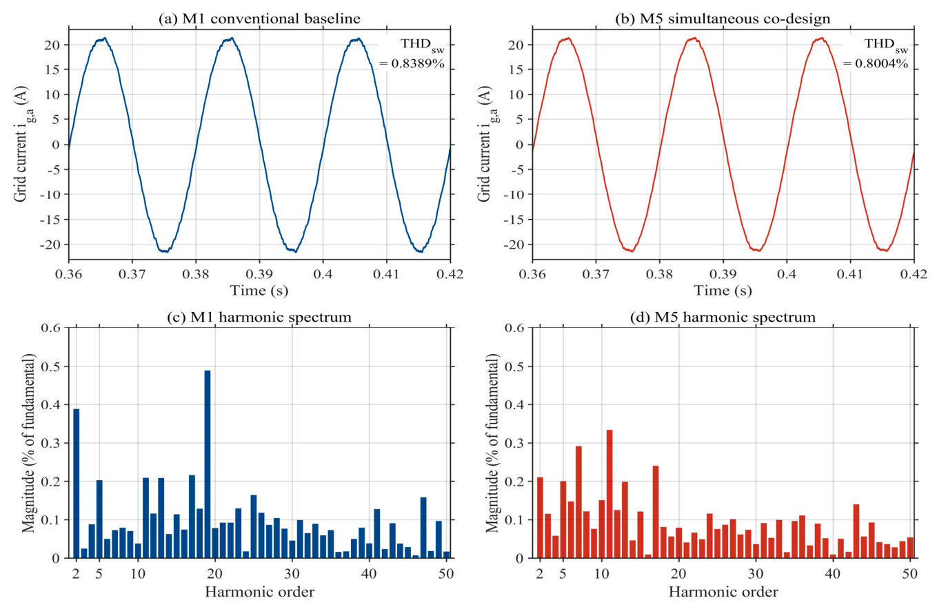
The resulting steady-state current waveforms and harmonic spectra are further visualized in the following comparison figure to provide direct waveform-level evidence of the switching-domain evaluation.

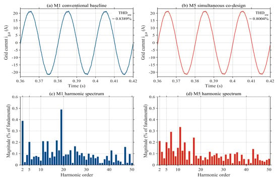
Figure 4 provides a waveform-level comparison between the conventional M1 design and the selected M5 design. Both the current waveform and harmonic spectrum are obtained using the same deterministic switching-domain evaluation procedure. The results reproduce the THD_sw values listed in Table 3 and provide direct waveform-level evidence for the switching-performance comparison.

Figure 4. Switching-domain comparison between the conventional M1 design and the selected M5 design using the same deterministic switching-function-based evaluator: (a) phase-a steady-state grid-current waveform for M1; (b) phase-a steady-state grid-current waveform for M5; (c) harmonic spectrum from the 2nd to 50th order for M1; and (d) harmonic spectrum from the 2nd to 50th order for M5.

3.6. Monte Carlo Robustness Assessment

The unified robustness experiment uses 1000 shared samples generated with rng(20260721, ‘twister’). For every method, L₁, L₂, C_f, R_d, K_p, K_r, and K_a are varied by ±10% around the nominal value of each finalized design; L_g is sampled from 0.1 to 3.0 mH, R_g from 0.05 to 0.40 Ω, and T_d from 1.0 to 2.0 T_s.The ±10% perturbation applied to the finalized design parameters is used as a prescribed engineering uncertainty range for comparative stress testing. It is not intended to represent a specific manufacturer tolerance. All normalized parameter perturbations are sampled independently from uniform distributions over their prescribed ranges. The same normalized perturbation samples and grid-delay samples are applied to M1–M5 so that differences in acceptance ratio reflect the design strategies rather than different random uncertainty realizations. The 95% confidence intervals for the strict acceptance ratios were calculated using the exact Clopper–Pearson binomial confidence interval.

The uncertainty ranges are selected as engineering stress-test intervals rather than a claim that every physical component has the same catalog tolerance. For L₁, L₂, C_f, and R_d, the +/−10% interval represents a common comparison envelope that can include manufacturing spread together with temperature, aging, and parameter-identification effects. The +/−10% controller-gain perturbations represent implementation and calibration sensitivity rather than component manufacturing tolerance. Variations in L_g, R_g, and T_d separately represent grid-strength and digital-delay uncertainty. Independent uniform sampling is retained to provide an identical controlled stress test for M1–M5; hardware-specific qualification would instead require the actual datasheet tolerances, distributions, and correlations of the selected components.

A sample passes the strict criterion only when all discrete poles lie inside the unit circle, all-crossover PM is at least 45°, all-crossover GM is at least 6 dB, and the modulation index does not exceed 0.98 with zero saturation. THD is not part of this Monte Carlo stability criterion. For M5, every failed row is independently cross-checked with all-margin and a discrete-pole audit.

4. Results and Discussion

4.1. Baseline Comparison

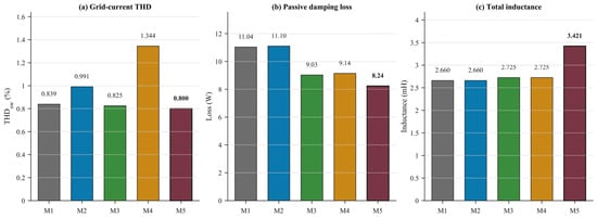
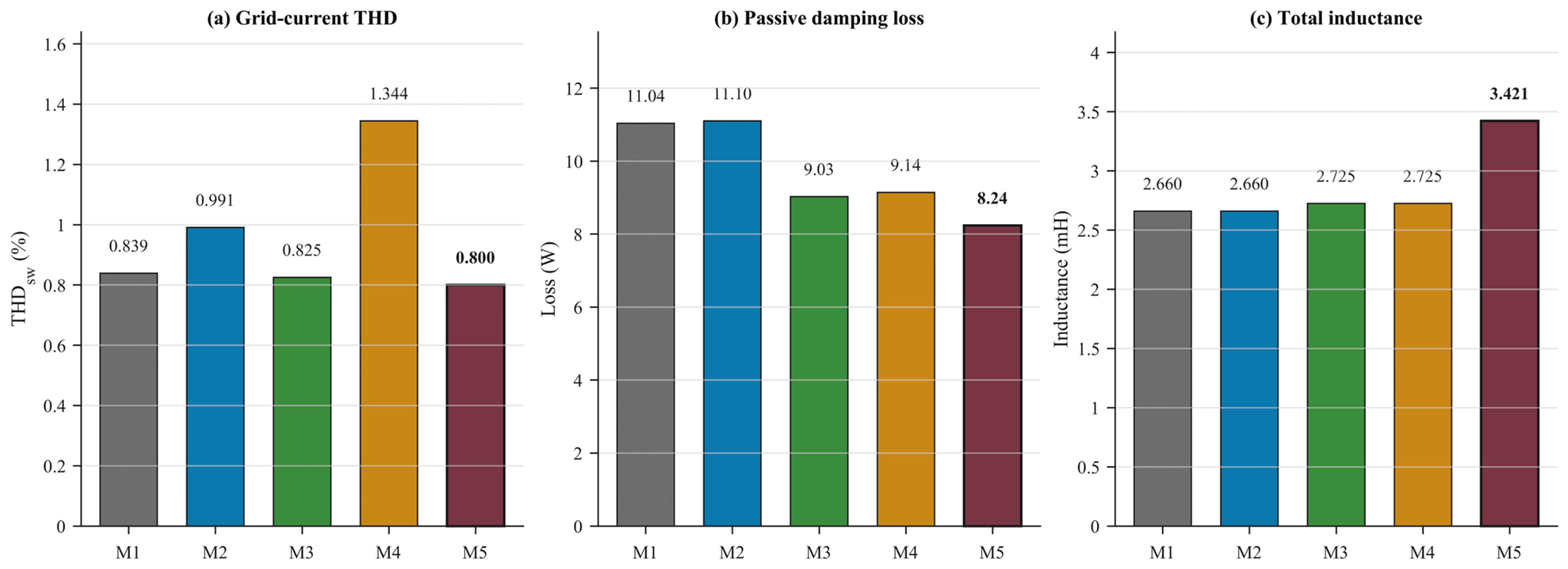
Table 3 compares the five design strategies using the same switching and robustness evaluation protocols. The reported worst stability margins are obtained from the common Cartesian audit over grid resistance, grid inductance, and digital delay. Figure 5 visualizes the switching THD, passive loss, and inductance comparison.

Figure 5. Comparison among M1–M5 of (a) switching-model grid-current THD; (b) passive damping loss; and (c) total inductance.

Numerical precision is standardized by quantity throughout the comparison: design parameters, passive loss, total inductance, and ITAE are reported to three decimal places; THD_sw is reported to four decimal places; stability margins are reported to two decimal places; and ratios are reported to one decimal place unless additional digits are required to reproduce an algorithmic setting. Table 1 retains engineering precision appropriate to each implementation parameter.

4.2. Effect of Controller Optimization

The M2 optimization decision vector is [K_p, K_r, K_a], with K_a searched over the same 0–10 range stated in Table 2. The selected Pareto compromise converges to the lower bound K_a = 0.000; therefore, the finalized M2 design differs from M1 only in K_p and K_r, rather than because K_a was excluded from the search. Relative to M1, nominal PM increases from 53.26 degrees to 59.61 degrees and nominal GM from 6.04 to 7.75 dB. The strict Monte Carlo acceptance ratio increases from 83.1% to 99.2%. This demonstrates a stability benefit from controller optimization. It does not improve every metric: THD_sw increases from 0.8389% to 0.9906%, ITAE increases, and passive damping loss remains approximately 11.1 W because the topology is fixed.

4.3. Effect of Passive-Network Parameter Optimization

M3 fixes the M1 controller exactly and modifies only L₁, L₂, C_f, and R_d. THD_sw decreases from 0.8389% to 0.8249%, and passive damping loss decreases from 11.036 W to 9.029 W, while total inductance increases from 2.660 to 2.725 mH. The Monte Carlo acceptance ratio also rises to 91.6%, although the worst PM and GM remain below the prescribed 45° and 6 dB gates. The passive-network-only result therefore improves passive harmonic/loss performance without providing the margin performance obtained by controller tuning.

4.4. Sequential Optimization Analysis

M4 applies passive-network parameter optimization first and controller optimization second. It has the largest nominal margins among the five strategies, PM = 69.02° and GM = 11.82 dB, and passes all 1000 strict Monte Carlo samples. This robustness is accompanied by a conservative performance trade-off: THD_sw is 1.3442%, ITAE is 3.322 × 10⁻⁵ A·s², power factor is 0.9918, and passive damping loss is 9.142 W. Because the second-stage controller is restricted to the topology selected in Stage 1, M4 cannot explore the same coupled design space as M5.

4.5. Proposed Simultaneous Co-Design

M5 simultaneously selects L₁ = 2.7849 mH, L₂ = 0.6364 mH, C_f = 5.8632 μF, R_d = 4.6063 Ω, K_p = 9.3996, K_r = 20.9242, and K_a = 4.6250. Compared with M1, THD_sw decreases by 4.6% and passive damping loss by 25.4%. Inverter-side and grid-side ripple decrease by 33.5% and 27.3%, respectively. These benefits require a 28.6% increase in total inductance.

The absolute THD_sw change from M1 to M5 is 0.0385 percentage points, so the harmonic improvement is modest and does not by itself justify the 0.761 mH (28.6%) increase in total inductance. The engineering rationale is instead multi-metric: passive damping loss decreases by 2.800 W (25.4%), inverter-side and grid-side ripple decrease by 33.5% and 27.3%, and nominal PM/GM improve by 5.87 degrees and 2.09 dB. More importantly, the worst PM/GM increases from 35.53 degrees/3.98 dB to 48.65 degrees/6.49 dB, thereby crossing the prescribed 45-degree/6 dB gates, while the strict Monte Carlo acceptance ratio rises from 83.1% to 98.3%. The nominal ITAE increases by about 4.7%, which confirms that M5 is a selected compromise with a larger magnetic requirement rather than an across-the-board improvement.

M5 gives a nominal PM/GM of 59.13°/8.13 dB and a worst PM/GM of 48.65°/6.49 dB. Its power factor is 0.9972, the maximum modulation index is 0.9153, and the saturation duration is zero. M5 is not the most robust method in the Monte Carlo comparison, because M4 reaches 100%; it is selected because it combines lower switching THD and passive loss with near-baseline ITAE and margins above the prescribed gates. The result is therefore a balanced improvement without claiming an improvement in every metric.

Although M4 achieves a higher strict robustness acceptance ratio, its sequential optimization nature leads to a more conservative design with increased switching THD and transient-performance degradation. The purpose of M5 is therefore not to maximize robustness margin alone, but to coordinate harmonic quality, damping loss, dynamic response, and robustness within the same coupled design space.

This comparison indicates that robustness margin alone is insufficient for the overall LCL-filtered inverter design. A highly conservative sequential design may improve stability margins at the expense of harmonic performance and dynamic behavior. The simultaneous co-design strategy therefore targets a balanced feasible region among harmonic quality, damping loss, transient response, and robustness.

Mechanism of Passive–Active Coupling

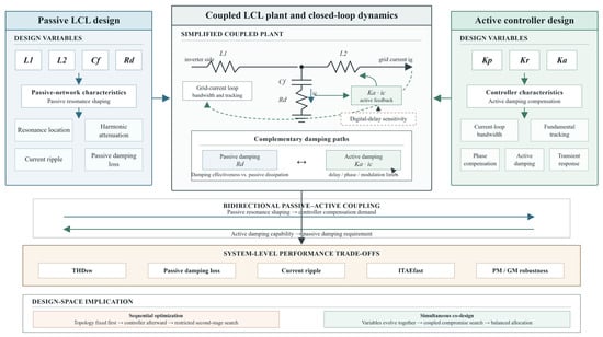
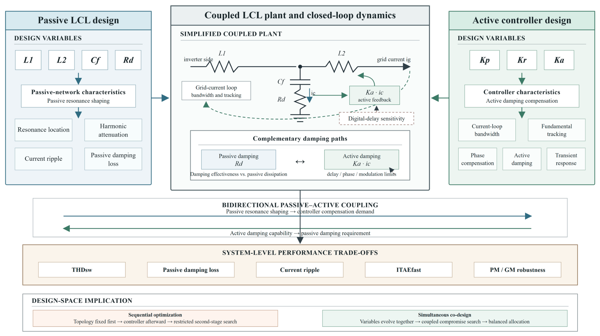
LCL-filter performance is jointly determined by passive resonance characteristics, active damping capability, and controller-bandwidth compatibility. The passive filter parameters reshape the frequency-domain plant characteristics, while the controller parameters determine the available compensation capability. Because each variable group changes the design requirements of the other, optimizing them independently can produce less balanced compromises even when each isolated design stage is feasible. Figure 6 illustrates the bidirectional coupling considered in the co-design: passive LCL parameters reshape the resonance and damping requirements seen by the controller, while controller bandwidth and active damping capability affect the feasible passive-network compromise.

Figure 6. Schematic illustration of passive–active coupling in the LCL-filter co-design, showing how passive-network parameters and controller parameters jointly affect resonance shaping, damping allocation, dynamic response, and robustness-related performance. Blue, gray, green, and beige regions denote passive design, the coupled plant, active control, and system-level trade-offs, respectively; arrows indicate the directions of influence and coupling.

Passive topology influence on system dynamics. Changes in L₁, L₂, and C_f shift the resonance frequency, modify harmonic attenuation, and alter inverter-side and grid-side current-ripple characteristics. The M3 passive-network-only result demonstrates that passive performance can be improved through these variables. However, because the controller parameters remain fixed, the achievable balance between stability and performance remains limited by the unchanged compensation capability.

Controller compensation and active damping coordination. K_p, K_r, and K_a determine controller bandwidth, resonant tracking, phase compensation, transient response, and active damping strength. The controller therefore cannot be designed independently of the LCL resonance characteristics presented by the plant. M2 improves stability through controller tuning, but the passive resonance characteristics remain unchanged because the LCL topology is fixed.

Coordination between passive and active damping. The series damping resistor R_d and capacitor current feedback gain K_a provide complementary damping paths. Increasing R_d can improve passive damping but also raises the passive damping-loss penalty. Increasing K_a can strengthen active damping and compensate resonance without relying exclusively on passive dissipation, but its useful range remains constrained by phase, delay, bandwidth, and modulation limits. Simultaneous co-design can therefore balance damping effectiveness against loss, whereas a sequential procedure may settle on a more conservative allocation because R_d and K_a are adjusted in different stages.

Sequential optimization first determines one subsystem and then compensates the other. Since the second optimization stage operates on a restricted design space, part of the topology-controller interaction information is no longer available to the joint search. M4 remains an effective baseline, but it is less flexible than simultaneous co-design. In M5, passive and active variables evolve together, allowing the search to identify compromise solutions rather than sequentially corrected solutions.

The improvement of M5 therefore does not originate merely from increasing the number of optimization variables. Instead, it results from explicitly considering the coupled relationship between passive resonance shaping and active damping compensation.

From the optimization results, the coupling effect can also be observed from the coordinated variation in passive and active damping variables. Compared with M3, the simultaneous design modifies both R_d and K_a, indicating that damping allocation is no longer limited to passive dissipation alone. The increase in active damping capability enables a different passive-network compromise, reducing damping loss while maintaining acceptable stability margins. The associated variable-level interpretation is summarized in Table 4.

Table 4. Interpretation of passive–active coupling mechanisms.

Variable	Primary Influence	Coupled Effect
L1/L2	Resonance shaping	Changes controller compensation requirement
Cf	Ripple attenuation	Changes active damping demand
Rd	Passive damping	Loss-performance trade-off
Ka	Active damping	Allows lower passive dissipation

Table 4. Interpretation of passive–active coupling mechanisms.

Variable	Primary Influence	Coupled Effect
L1/L2	Resonance shaping	Changes controller compensation requirement
Cf	Ripple attenuation	Changes active damping demand
Rd	Passive damping	Loss-performance trade-off
Ka	Active damping	Allows lower passive dissipation

4.6. Computational Role of GPR-Assisted Screening

Direct switching-function evaluation is computationally expensive when applied to a large Pareto archive. The surrogate model is introduced only as a computational acceleration tool for candidate screening. It does not define the optimization objective, replace the high-fidelity switching model, or determine the final design independently. Its held-out performance is reported in Table 5.

Table 5. GPR screening performance on validation and independent test sets.

Dataset	n	R2	RMSE (Percentage Points)	MAE (Percentage Points)	Spearman	Pearson
Validation	22	0.7327	0.1009	0.0801	0.8701	0.8576
Independent test	22	0.6557	0.1638	0.1374	0.7708	0.8307

Note: The independent test set is excluded from fitting, hyperparameter selection, and candidate ranking. Final M5 performance is obtained from direct switching simulation.

The surrogate model should be interpreted as a lightweight ranking mechanism. Its contribution is reflected in reducing the number of candidates requiring expensive switching-domain evaluation rather than replacing the physical model.

On the independent test split, the surrogate gives R² = 0.6557, RMSE = 0.1638 percentage points, and MAE = 0.1374 percentage points. These results characterize a moderate-fidelity approximation that provides screening capability and ranking assistance rather than a replacement for direct switching evaluation.

The retained candidate archive contains 2962 unseen feasible designs, of which 10 are sent to direct switching verification after GPR-assisted ranking. Thus, 2952 candidate-level switching evaluations are avoided, corresponding to 1 − 10/2962 = 99.66% fewer switching evaluations at this screening stage. This is an evaluation-count reduction, not a measured 99.66% reduction in total elapsed time. End-to-end runtime also includes archive generation, engineering filtering, feature preparation, GPR fitting and inference, the retained switching evaluations, and parallelization overhead; because those contributions were not timed as one controlled benchmark, no wall-clock acceleration factor is claimed.

Although the surrogate model reduces computational burden, final candidate acceptance still relies on independent switching verification and robustness assessment.

4.7. Unified Monte Carlo Robustness Assessment

Three complementary robustness indicators are considered: (1) the strict acceptance ratio, which applies the complete margin, pole, modulation, and saturation gates; (2) the true pole stability ratio, which identifies samples whose discrete closed-loop poles remain inside the unit circle; and (3) the effective margin anomaly ratio, which records conservative all-crossover rejections that do not coincide with true pole instability. Together, these indicators distinguish strict frequency-domain acceptance from closed-loop pole stability. Table 6 reports these indicators under the common uncertainty protocol.

Table 6. Monte Carlo robustness assessment under shared uncertainty samples.

Method	Samples	Strict Acceptance Ratio (%)	95% CI (%)	Minimum All-Crossover PM Indicator (°)	Worst Effective GM (dB)	True Pole Instability Ratio (%)	Margin Anomaly Ratio (%)
M1	1000	83.1	[80.6, 85.4]	32.92	3.37	0.0	16.9
M2	1000	99.2	[98.4, 99.7]	45.28	5.15	0.0	0.8
M3	1000	91.6	[89.7, 93.2]	34.85	3.84	0.0	8.4
M4	1000	100.0	[99.6, 100.0]	60.56	9.01	0.0	0.0
M5	1000	98.3	[97.3, 99.0]	−174.99	5.73	0.0	1.7

Note: The minimum all-crossover PM indicator is a conservative frequency-domain diagnostic and does not directly represent closed-loop instability. Discrete-pole analysis is therefore additionally performed to distinguish effective margin anomalies from true pole instability. For M5, the audit confirms zero true pole instability; the rejected cases are classified as conservative margin anomalies caused by multiple crossover conditions. PM is reported in degrees (°) and GM in dB. The same uncertainty samples and strict acceptance criteria were applied to all five strategies. For M5, the rejected samples were additionally examined using MATLAB’s all-margin and discrete-pole analysis to interpret the multiple-crossover anomalies; this additional audit did not alter the original strict acceptance classification.

The shared uncertainty samples ensure that the comparison reflects differences among design strategies rather than different random realizations.

The minimum all-crossover PM indicator originates from a secondary crossover condi-tion under the all-crossover criterion. Although this criterion provides a conservative frequency-domain evaluation, discrete pole analysis confirms zero true pole instability among the Monte Carlo samples.

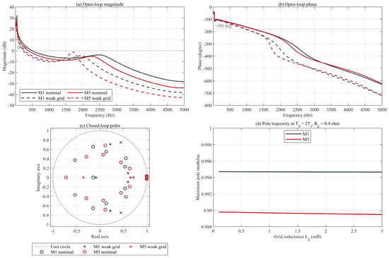
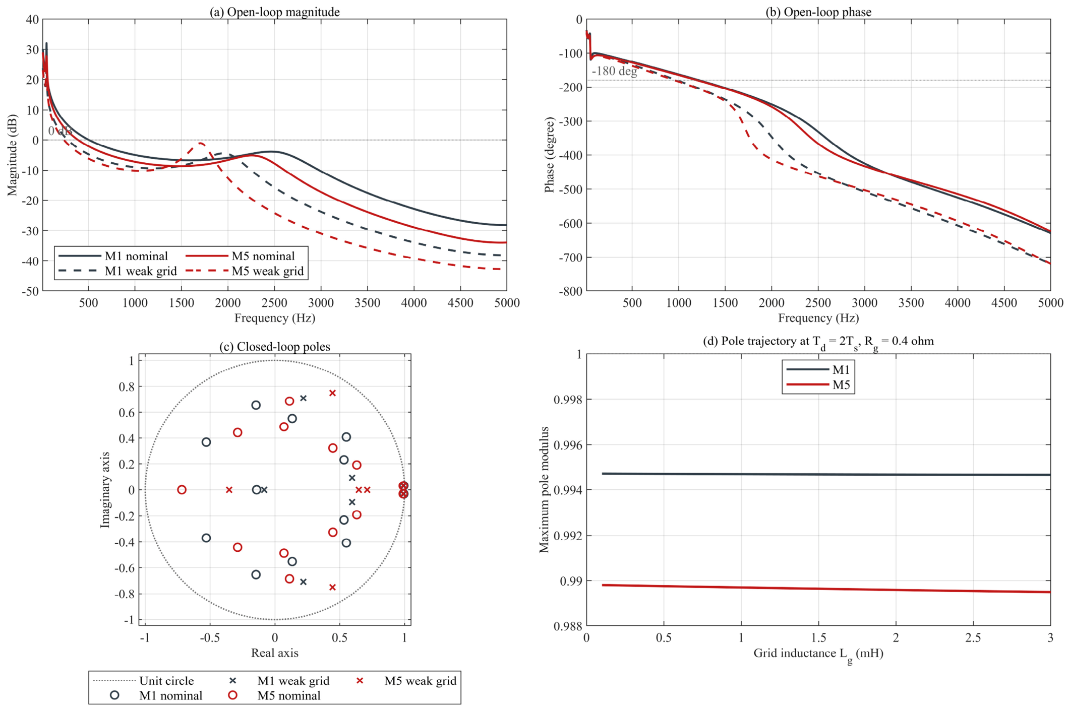
To complement the scalar margins in Table 6, Figure 7 compares representative open-loop Bode responses and discrete closed-loop poles for the frozen M1 and M5 designs. The nominal case uses L_g = 0.5 mH, R_g = 0.1 ohm, and T_d = 1.5 T_s; the weak-grid maximum-delay case uses L_g = 3 mH, R_g = 0.4 ohm, and T_d = 2 T_s. The pole trajectory panel further sweeps L_g from 0.1 to 3 mH at T_d = 2 T_s and R_g = 0.4 ohm. All curves use the unified LCL plant, method-specific frozen controllers, and the exact frequency-domain delay response.

Figure 7. Representative frequency-domain and closed-loop pole comparison for the frozen M1 and M5 designs: (a) open-loop magnitude; (b) open-loop phase; (c) nominal and weak-grid discrete poles; and (d) maximum-pole-modulus trajectory versus grid inductance at T_d = 2 T_s and R_g = 0.4 ohm.

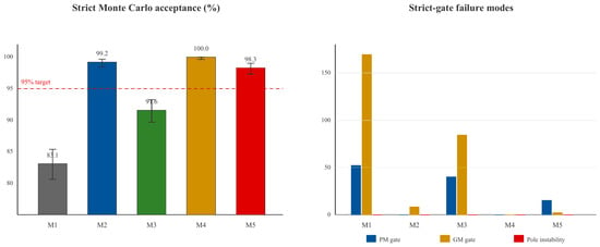
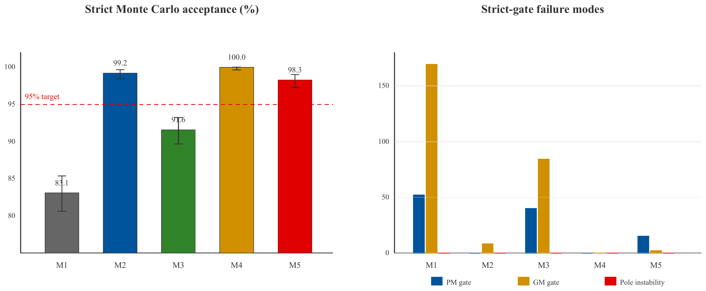
Figure 8 reports the shared-sample acceptance and gate-failure counts.

Figure 8. Monte Carlo robustness assessment under shared uncertainty samples.

The shared strict acceptance ratios are 83.1%, 99.2%, 91.6%, 100.0%, and 98.3% for M1–M5, respectively. The proposed M5 design achieves a high strict acceptance ratio within the investigated uncertainty domain. Its 17 strict failures comprise 15 PM-gate failures and two GM-gate failures. All 17 samples retain poles inside the unit circle and are reproduced by direct all-margin evaluation, giving a true pole-instability ratio of 0% and an effective margin anomaly ratio of 1.7%.

The reported minimum all-crossover PM indicator of −174.99° occurs at a secondary gain crossover in a multiple-crossover sample. It is neither a phase-processing error nor evidence of a discrete pole outside the unit circle. The original 98.3% strict acceptance ratio is retained, while the pole audit shows that the observed rejections are effective-margin anomalies under the conservative all-crossover criterion rather than true pole instability.

5. Engineering Implications and Limitations

5.1. Passive Damping and Magnetic Utilization

M5 reduces the modeled capacitor-branch damping loss from 11.036 W to 8.236 W, a 25.4% reduction. This result indicates lower auxiliary damping dissipation in the modeled operating condition, but it is not a complete converter-efficiency calculation. Semiconductor conduction and switching energies, magnetic core and copper losses, thermal behavior, and auxiliary consumption are not modeled.

The M5 total inductance increases from 2.660 mH to 3.421 mH. Consequently, the study does not claim reduced magnetic volume or cost. Instead, it exposes the quantified trade-off between magnetic requirement, damping loss, current ripple, dynamic response, and robust stability.

5.2. Applicability to Renewable Integration

Coordinating passive and active design variables helps maintain acceptable margins over the investigated grid-impedance and delay domain while limiting harmonic current and passive loss. This supports reliable PV integration under uncertain grid conditions within the validated model scope. It is not a complete low-voltage-ride-through or grid-code compliance demonstration.

5.3. Limitations

The DC source is ideal, and the model omits PV-array dynamics, MPPT, the DC-link voltage loop, semiconductor switching transients, dead time, magnetic nonlinearity, detailed device losses, and thermal effects. The inverter is represented by a switching function rather than a device-level power stage. The GPR model is calibrated on a finite design domain and must not be extrapolated. The Monte Carlo study estimates performance under the stated distributions and is not a proof over every continuous uncertainty combination. Reactive-power operation and low-voltage ride-through require separate controller validation. Hardware-in-the-loop and experimental hardware validation will be conducted in future work.

6. Conclusions

A five-strategy comparative study was conducted under a common plant, delay, modulation, switching, FFT, and Monte Carlo protocol. Control-only optimization improved nominal margins and the strict uncertainty acceptance ratio relative to M1, although it did not improve harmonic or passive-loss metrics. Passive-network-only optimization reduced switching THD and damping loss while retaining the M1 controller, but its worst margins remained below the prescribed gates.

Sequential topology-then-control optimization was effective for robustness and passed all 1000 strict samples, but it produced a conservative trade-off in switching THD, power factor, and ITAE. The simultaneous co-design produced the selected compromise design among the evaluated strategies. The proposed framework improves the overall trade-off among harmonic quality, damping loss, dynamic performance, and uncertainty tolerance. M5 combined THD_sw = 0.8004%, damping loss = 8.236 W, near-baseline ITAE, nominal PM/GM of 59.13°/8.13 dB, and worst PM/GM above 45°/6 dB, while accepting a larger total inductance than M1.

The leakage-free GPR surrogate reduced candidate switching evaluations by 99.66%, but its independent-test errors confirm that it should remain a screening accelerator. Direct switching verification remains the final harmonic-performance gate. The M5 Monte Carlo strict acceptance ratio is 98.3%, with zero true discrete-pole instability and a 1.7% effective margin anomaly ratio; the conclusion is therefore probabilistic, and M5 is described as robust within the investigated uncertainty domain. Future work will add HIL and hardware experiments, device-level loss analysis, and broader grid-support control validation.

References

- Twining, E.; Holmes, D.G. Grid current regulation of a three-phase voltage source inverter with an LCL input filter. IEEE Trans. Power Electron. 2003, 18, 888–895. [Google Scholar] [CrossRef] [Scilit]
- Liserre, M.; Blaabjerg, F.; Hansen, S. Design and Control of an LCL-Filter-Based Three-Phase Active Rectifier. IEEE Trans. Ind. Appl. 2005, 41, 1281–1291. [Google Scholar] [CrossRef] [Scilit]
- Liserre, M.; Teodorescu, R.; Blaabjerg, F. Stability of photovoltaic and wind turbine grid-connected inverters for a large set of grid impedance values. IEEE Trans. Power Electron. 2006, 21, 263–272. [Google Scholar] [CrossRef] [Scilit]
- Blaabjerg, F.; Teodorescu, R.; Liserre, M.; Timbus, A.V. Overview of Control and Grid Synchronization for Distributed Power Generation Systems. IEEE Trans. Ind. Electron. 2006, 53, 1398–1409. [Google Scholar] [CrossRef] [Scilit]
- Teodorescu, R.; Blaabjerg, F.; Liserre, M.; Loh, P.C. Proportional-resonant controllers and filters for grid-connected voltage-source converters. IEE Proc. Electr. Power Appl. 2006, 153, 750–762. [Google Scholar] [CrossRef] [Scilit]
- Sun, J. Impedance-Based Stability Criterion for Grid-Connected Inverters. IEEE Trans. Power Electron. 2011, 26, 3075–3078. [Google Scholar] [CrossRef] [Scilit]
- Balasubramanian, A.K.; John, V. Analysis and design of split-capacitor resistive-inductive passive damping for LCL filters in grid-connected inverters. IET Power Electron. 2013, 6, 1822–1832. [Google Scholar] [CrossRef] [Scilit]
- Pan, D.; Ruan, X.; Bao, C.; Li, W.; Wang, X. Capacitor-Current-Feedback Active Damping With Reduced Computation Delay for Improving Robustness of LCL-Type Grid-Connected Inverter. IEEE Trans. Power Electron. 2014, 29, 3414–3427. [Google Scholar] [CrossRef] [Scilit]
- Bao, C.; Ruan, X.; Wang, X.; Li, W.; Pan, D.; Weng, K. Step-by-Step Controller Design for LCL-Type Grid-Connected Inverter with Capacitor–Current-Feedback Active-Damping. IEEE Trans. Power Electron. 2014, 29, 1239–1253. [Google Scholar] [CrossRef] [Scilit]
- Xu, J.; Xie, S.; Tang, T. Active damping-based control for grid-connected LCL-filtered inverter with injected grid current feedback only. IEEE Trans. Ind. Electron. 2014, 61, 4746–4758. [Google Scholar] [CrossRef] [Scilit]
- Zhang, C.; Li, Y.; Jia, C.; Fu, H.; Zhang, X.; Zhang, H. Direct active damping control for grid-connected AC/DC converter with LCL filter using augmented look-up table. IET Power Electron. 2021, 14, 1089–1101. [Google Scholar] [CrossRef] [Scilit]
- Jayalath, S.; Hanif, M. Generalized LCL-Filter Design Algorithm for Grid-Connected Voltage-Source Inverter. IEEE Trans. Ind. Electron. 2017, 64, 1905–1915. [Google Scholar] [CrossRef] [Scilit]
- Liu, J.; Zhou, L.; Molinas, M. Damping region extension for digitally controlled LCL-type grid-connected inverter with capacitor-current feedback. IET Power Electron. 2018, 11, 1974–1982. [Google Scholar] [CrossRef] [Scilit]
- Xu, J.; Xie, S.; Zhang, B.; Qian, Q. Robust Grid Current Control With Impedance-Phase Shaping for LCL-Filtered Inverters in Weak and Distorted Grid. IEEE Trans. Power Electron. 2018, 33, 10240–10250. [Google Scholar] [CrossRef] [Scilit]
- He, Y.; Chung, H.-S.-H.; Lai, C.-T.; Zhang, X.; Wu, W. Active Cancelation of Equivalent Grid Impedance for Improving Stability and Injected Power Quality of Grid-Connected Inverter Under Variable Grid Condition. IEEE Trans. Power Electron. 2018, 33, 9387–9398. [Google Scholar] [CrossRef] [Scilit]
- Zhou, X.; Zhou, L.; Chen, Y.; Shuai, Z.; Guerrero, J.M.; Luo, A.; Wu, W.; Yang, L. Robust Grid-Current-Feedback Resonance Suppression Method for LCL-Type Grid-Connected Inverter Connected to Weak Grid. IEEE J. Emerg. Sel. Top. Power Electron. 2018, 6, 2126–2137. [Google Scholar] [CrossRef] [Scilit]
- He, Y.; Wang, X.; Ruan, X.; Pan, D.; Xu, X.; Liu, F. Capacitor-Current Proportional-Integral Positive Feedback Active Damping for LCL-Type Grid-Connected Inverter to Achieve High Robustness Against Grid Impedance Variation. IEEE Trans. Power Electron. 2019, 34, 12423–12436. [Google Scholar] [CrossRef] [Scilit]
- Kim, Y.-J.; Kim, H. Optimal design of LCL filter in grid-connected inverters. IET Power Electron. 2019, 12, 1774–1782. [Google Scholar] [CrossRef] [Scilit]
- Cai, Y.; He, Y.; Zhou, H.; Liu, J. Design Method of LCL Filter for Grid-Connected Inverter Based on Particle Swarm Optimization and Screening Method. IEEE Trans. Power Electron. 2021, 36, 10097–10113. [Google Scholar] [CrossRef] [Scilit]
- Sgrò, D.; Souza, S.A.; Tofoli, F.L.; Leão, R.P.S.; Sombra, A.K.R. An integrated design approach of LCL filters based on nonlinear inductors for grid-connected inverter applications. Electr. Power Syst. Res. 2020, 186, 106389. [Google Scholar] [CrossRef] [Scilit]
- Ma, G.; Xie, C.; Li, C.; Peng, C.; Zou, J. Passivity-Based Design of External Passive Damper for LCL-Type Grid-Connected Inverter. IEEE Trans. Power Electron. 2024, 39, 11558–11570. [Google Scholar] [CrossRef] [Scilit]
- Ali, R.; Heydari-Doostabad, H.; Sajedi, S.; O’Donnell, T. Improved design of passive damping for single phase grid-connected LCL filtered inverter considering impedance stability. IET Power Electron. 2024, 17, 511–523. [Google Scholar] [CrossRef] [Scilit]
- Liu, X.; Liu, Y.; Yin, J. Magnetic integration of a symmetrical LCL filter in the grid-tied inverter with reduced EMI noise. IET Power Electron. 2024, 17, 1526–1539. [Google Scholar] [CrossRef] [Scilit]
- Zhu, D.; Zhou, S.; Zou, X.; Kang, Y. Improved Design of PLL Controller for LCL-Type Grid-Connected Converter in Weak Grid. IEEE Trans. Power Electron. 2020, 35, 4715–4727. [Google Scholar] [CrossRef] [Scilit]
- Xue, T.; Sun, P.; Xu, Z.; Luo, Q. Feedforward phase compensation method of LCL grid-connected inverter based on all-pass filter in grid-impedance condition. IET Power Electron. 2020, 13, 4407–4416. [Google Scholar] [CrossRef] [Scilit]
- Huang, L.; Wu, C.; Zhou, D.; Blaabjerg, F. A Double-PLLs-Based Impedance Reshaping Method for Extending Stability Range of Grid-Following Inverter Under Weak Grid. IEEE Trans. Power Electron. 2022, 37, 4091–4104. [Google Scholar] [CrossRef] [Scilit]
- Lin, X.; Yu, J.; Yu, R.; Zhang, J.; Yan, Z.; Wen, H. Improving Small-Signal Stability of Grid-Connected Inverter Under Weak Grid by Decoupling Phase-Lock Loop and Grid Impedance. IEEE Trans. Ind. Electron. 2022, 69, 7040–7053. [Google Scholar] [CrossRef] [Scilit]
- Quan, X. Improved Dynamic Response Design for Proportional Resonant Control Applied to Three-Phase Grid-Forming Inverter. IEEE Trans. Ind. Electron. 2021, 68, 9919–9930. [Google Scholar] [CrossRef] [Scilit]
- Alathamneh, M.; Ghanayem, H.; Yang, X.; Nelms, R.M. Three-Phase Grid-Connected Inverter Power Control under Unbalanced Grid Conditions Using a Proportional-Resonant Control Method. Energies 2022, 15, 7051. [Google Scholar] [CrossRef] [Scilit]
- He, S.; Xiong, J.; Wang, Z.; Lin, S. Robust AD for LCL-type grid-connected inverter with capacitor current quasi-integral feedback. IET Power Electron. 2020, 13, 1332–1342. [Google Scholar] [CrossRef] [Scilit]
- Li, S.; Lin, H. A Capacitor-Current-Feedback Positive Active Damping Control Strategy for LCL-Type Grid-Connected Inverter to Achieve High Robustness. IEEE Trans. Power Electron. 2022, 37, 6462–6474. [Google Scholar] [CrossRef] [Scilit]
- Liu, J.; Zhang, X.; Wang, B. Wide-Band Harmonic Resonance Damping Strategy for Grid-Connected Digitally Controlled LCL-Type Inverter. IET Power Electron. 2025, 18, e70126. [Google Scholar] [CrossRef] [Scilit]
- He, Y.; Wang, X.; Ruan, X.; Pan, D.; Qin, K. Hybrid Active Damping Combining Capacitor Current Feedback and Point of Common Coupling Voltage Feedforward for LCL-Type Grid-Connected Inverter. IEEE Trans. Power Electron. 2021, 36, 2373–2383. [Google Scholar] [CrossRef] [Scilit]
- Jia, X.; Yu, S.; Zhang, Y.; Feng, Y.; Zhou, B. LCL Grid-Connected Inverter Resonance Feedforward-Active Damping Hybrid Control Strategy for Mitigating Weak Grid Resonance and Harmonic Currents. Energies 2025, 18, 6010. [Google Scholar] [CrossRef] [Scilit]
- Wang, A.; Guo, Z.; Li, Z.; Zhang, J.; Wu, X.; Tan, G. Hybrid active damping based on fixed-gain capacitor current positive feedback and unit capacitor voltage positive feedback for LCL-type grid-connected inverter. IEEE J. Emerg. Sel. Top. Power Electron. 2026. early access. [Google Scholar] [CrossRef] [Scilit]
- Hu, Z.; Xing, X.; Wang, H.; Li, Z.; Li, Y.; Blaabjerg, F. Modeling and Delay Compensation Method for Improving the Stability of Grid-Connected Inverter With LCL Filter Under Weak Grid Conditions. IEEE Trans. Power Electron. 2026, 41, 6111–6124. [Google Scholar] [CrossRef] [Scilit]
- Zhu, J.; Zhou, B.; Li, Y.; Peng, F.Z.; Lehman, B. Generalized direct grid current control for voltage sensorless grid-connected inverter with output LCL filter. IEEE Trans. Power Electron. 2026. early access. [Google Scholar] [CrossRef] [Scilit]
- Lyu, J.; Yan, Y.; Wu, F.; Sun, Z.; Farooq, A.; Xu, W. Parameter co-design of active damping loop and grid current controller for a 3-phase LCL-filtered grid-connected inverter. Int. J. Electr. Power Energy Syst. 2021, 133, 107203. [Google Scholar] [CrossRef] [Scilit]
- Fang, T.; Shen, S.; Jin, Y.; Ruan, X. Robustness Investigation of Multi-Inverter Paralleled Grid-Connected System With LCL-Filter Based on the Grid-Impedance Allocation Mechanism. IEEE Trans. Power Electron. 2021, 36, 14508–14524. [Google Scholar] [CrossRef] [Scilit]
- Chen, Y.; Sangwongwanich, A.; Huang, M.; Pan, S.; Zha, X.; Wang, H. Failure Risk Assessment of Grid-Connected Inverter With Parametric Uncertainty in LCL Filter. IEEE Trans. Power Electron. 2023, 38, 9514–9525. [Google Scholar] [CrossRef] [Scilit]
- Rashidi, N.; Wang, Q.; Burgos, R.; Roy, C.; Boroyevich, D. Multi-objective Design and Optimization of Power Electronics Converters With Uncertainty Quantification—Part I: Parametric Uncertainty. IEEE Trans. Power Electron. 2021, 36, 1463–1474. [Google Scholar] [CrossRef] [Scilit]
- Liu, J.; Sun, X.; Chen, Z.; Chi, Y.; Song, W.; Zhu, Q.; Wheeler, P. A Hybrid Multiresonances Suppression Method for Nonsynchronous LCL-Type Grid-Connected Inverter Clusters Under Weak Grid. IEEE Trans. Power Electron. 2024, 39, 5386–5399. [Google Scholar] [CrossRef] [Scilit]
- Amorim, T.S.; Carletti, D.; Sepulchro, W.N.; Encarnação, L.F. Decentralized inverter control with selective harmonic damping connected to a multi-bus grid. Electr. Power Syst. Res. 2026, 251, 112318. [Google Scholar] [CrossRef] [Scilit]
- Sui, Z.; Sun, Q.; Wang, R.; Li, D.; Wang, P. The Grid-Connected Inverter Stability Enhancement Control Based on Impedance Instability Region Elimination. IEEE Trans. Power Electron. 2025, 40, 9606–9624. [Google Scholar] [CrossRef] [Scilit]
- Xie, C.; Li, K.; Zou, J.; Guerrero, J.M. Passivity-Based Stabilization of LCL-Type Grid-Connected Inverters via a General Admittance Model. IEEE Trans. Power Electron. 2020, 35, 6636–6648. [Google Scholar] [CrossRef] [Scilit]
- Zhang, H.; Tao, R.; Li, Z.; Zhang, X.; Ma, Z. Multivariable sequential model predictive control of LCL-type grid connected inverter. IET Power Electron. 2023, 16, 558–574. [Google Scholar] [CrossRef] [Scilit]
- Cho, N.; Wendha, B.; Luthfi, M. Evaluations on the harmonic allocation methods of IEC 61000-3-6 and IEEE Standard 519 in the distribution systems. Electr. Power Syst. Res. 2024, 230, 110260. [Google Scholar] [CrossRef] [Scilit]
- Jones, D.R.; Schonlau, M.; Welch, W.J. Efficient Global Optimization of Expensive Black-Box Functions. J. Glob. Optim. 1998, 13, 455–492. [Google Scholar] [CrossRef] [Scilit]
- Shahriari, B.; Swersky, K.; Wang, Z.; Adams, R.P.; de Freitas, N. Taking the Human Out of the Loop: A Review of Bayesian Optimization. Proc. IEEE 2016, 104, 148–175. [Google Scholar] [CrossRef] [Scilit]
- Cong, H.; Wang, B.; Wang, Z. A Novel Gaussian Process Surrogate Model with Expected Prediction Error for Optimization under Constraints. Mathematics 2024, 12, 1115. [Google Scholar] [CrossRef] [Scilit]
- Khatouri, H.; Benamara, T.; Breitkopf, P.; Demange, J. Metamodeling techniques for CPU-intensive simulation-based design optimization: A survey. Adv. Model. Simul. Eng. Sci. 2022, 9, 1. [Google Scholar] [CrossRef] [Scilit]
- Deb, K.; Pratap, A.; Agarwal, S.; Meyarivan, T. A fast and elitist multiobjective genetic algorithm: NSGA-II. IEEE Trans. Evol. Comput. 2002, 6, 182–197. [Google Scholar] [CrossRef] [Scilit]
- IEEE Std 1547-2018; IEEE Standard for Interconnection and Interoperability of Distributed Energy Resources with Associated Electric Power Systems Interfaces. IEEE: Piscataway, NJ, USA, 2018. [Google Scholar] [CrossRef] [Scilit]
- IEEE Std 519-2022; IEEE Standard for Harmonic Control in Electric Power Systems. IEEE: Piscataway, NJ, USA, 2022. [Google Scholar] [CrossRef] [Scilit]
Disclaimer/Publisher’s Note: The statements, opinions and data contained in all publications are solely those of the individual author(s) and contributor(s) and not of MDPI and/or the editor(s). MDPI and/or the editor(s) disclaim responsibility for any injury to people or property resulting from any ideas, methods, instructions or products referred to in the content. |
© 2026 by the authors. Licensee MDPI, Basel, Switzerland. This article is an open access article distributed under the terms and conditions of the Creative Commons Attribution (CC BY) license.