A Polynomial Regression-Based Approach for Efficiency and Performance Trend Monitoring of Hydropower Turbines

Abstract

Hydropower plays an increasingly important role in sustainable energy systems. While efficient plant operation is essential, hydropower efficiency is often assessed only during commissioning or over short measurement periods, leaving long-term trends largely unexplored. This limits the early detection of performance degradation and reduces opportunities for timely maintenance and optimization. To address this gap, this paper presents a framework for continuous efficiency trend monitoring based on polynomial regression, combined with measurement uncertainty analysis to distinguish genuine performance changes from noise. Particular attention is given to data preprocessing and aggregation. The resulting regression models used to estimate turbine efficiency from operational and discharge measurements achieved root mean square error (RMSE) values between 0.149% and 0.176%. An alternative model that predicts power output from head and guide vane opening yielded an RMSE of 0.28% in the most frequently used operating range. The resulting residuals were tracked over time and remained within the confidence levels defined by measurement uncertainty. Seasonal effects were also evident in the results, demonstrating the potential of the proposed approach for long-term monitoring of hydropower plant performance.

1. Introduction

With a 14% share in global electricity production in 2025, hydropower remains a cornerstone of the global transition toward sustainable and low-carbon energy systems [1]. The reliable and efficient operation of hydropower plants is crucial not only for maximizing energy output but also for reducing environmental impacts and operational costs. However, the efficiency and operational lifespan of hydropower turbines can deteriorate over time due to various factors such as sedimentation, mechanical wear, and fluctuating operational conditions [2].

Continuous monitoring of turbine efficiency is therefore essential to detect performance degradation at an early stage and enable timely maintenance interventions. Traditional efficiency assessments often rely on intermittent measurements conducted during scheduled inspections or standardized tests at fixed intervals [3]. While these periodic evaluations provide snapshots of plant performance, they may fail to capture subtle or gradual efficiency declines occurring over longer timescales, thereby limiting the plant operator’s ability to optimize performance and manage risks effectively. Moreover, measurement uncertainty—arising from instrumentation limitations, environmental variability, and data processing techniques—can mask genuine efficiency trends and complicate the interpretation of monitoring results [4].

This study presents a regression-based framework for continuous monitoring of hydropower-plant efficiency trends. Uncertainties associated with the efficiency estimates are quantified and explicitly incorporated into the analysis. The framework is validated using operational data from a modern run-of-river hydropower plant in Northern Europe. Commissioned in 2014, the plant comprises two Kaplan turbine units, each rated at approximately 50 MW, and is representative of contemporary large-scale hydropower installations.

The investigation addresses the following research questions:

•

How can continuous, long-term monitoring of hydropower-turbine efficiency be implemented effectively?

•

Can operational process data yield statistically meaningful and accurate efficiency trends when measurement uncertainty is explicitly considered?

•

Are direct discharge measurements necessary to obtain statistically meaningful indicators of performance degradation?

The remainder of this paper is organized as follows. Section 2 reviews the current state of research on hydropower efficiency monitoring. Section 3 describes the methodology, including data preprocessing, regression modeling, and uncertainty propagation. Section 4 presents the application of the proposed framework to operational data and discusses the resulting findings. Section 5 summarizes the main conclusions and identifies directions for future research.

2. State of the Art

IEC 60041:1991 [3] provides an established and accepted international standard for warranty measurements. It is commonly applied to test the efficiency of a limited number of operating points or parts of the operating range at a given point in time. In this sense, such a specific turbine efficiency measurement represents only sort of a snapshot of the turbine performance in the context of refurbishments or completion of new hydropower plants. Long-term efficiency monitoring is neither scope nor object of this standard.

However, studies addressing long-term monitoring of hydropower generation remain scarce. Multi-year field data show that turbine efficiency losses correlate poorly with operating hours or sediment load and are hardly predictable, so continuous long-term monitoring is recommended [5]. Building on this, Abgottspon et al. [6] propose a continuous turbine-efficiency monitoring approach that incorporates input-data validation and the detection of quasi-steady operating conditions. Daily efficiency values are compared with a reference hill chart established through a comprehensive measurement campaign, thereby accounting for potential deviations between actual turbine efficiency and values derived from model tests or numerical simulations. The approach thus requires a dedicated measurement campaign to establish the reference.

Gloor and Staubli [7] describe a methodology for identifying quasi-steady operating conditions in turbine-efficiency monitoring and for validating input data through the automated detection and removal of outliers. The removal of anomalous observations reduces variability in the calculated performance indicators, resulting in more stable trends and greater confidence in turbine-condition assessment. However, the focus lies on data preparation rather than on the modeling of efficiency trends.

Amini et al. [8] studied the prediction of generated power at a hydropower unit with a hybrid physics-informed deep learning model, besides other approaches. Fluctuations observed in the raw data were specifically addressed. However, the study period spanned two weeks. A dedicated preprocessing of the raw data in terms of quasi-steady operation identification is not explicitly mentioned in the study.

Kumar et al. [9] predict the efficiency of a Kaplan unit from historical operating data using curve fitting, multiple linear regression, and artificial neural networks; the latter achieve a root mean square percentage error of 0.18%. Since the data are split randomly, changes over time are not analyzed, and measurement uncertainty is not considered. Additionally, discharge is the most influential input of their model, and the target efficiency is itself calculated from head, discharge, and power. Efficiency-based monitoring therefore depends on discharge, the quantity most difficult to measure in the field. In low-head plants, it is often determined by relative methods such as the Winter–Kennedy method, whose uncertainty can reach 5% [10].

Abgottspan et al. [11] highlight that records of efficiency, operating patterns, and energy-loss analysis are essential for cost-effective maintenance decisions, support rehabilitation specifications at the tender stage that avoid gaps between design and actual performance, and ultimately for reducing costs.

Existing approaches thus rely on reference measurements, short periods or discharge data, and none evaluates long-term trends against measurement uncertainty. The current paper therefore combines quasi-steady operation filtering, polynomial regression and uncertainty propagation for multi-year trend monitoring, including an alternative model without the need for discharge measurement.

3. Methodology

In line with the International Standard IEC 60041:1991 [3], the turbine efficiency is considered as

$$\eta ={\displaystyle \frac{P}{P_h}}$$

(1)

where

•

P is the mechanical power delivered by the turbine shaft, assigning to the hydraulic machine the mechanical losses of the relevant bearings through the coupling of the runner and the shaft;

•

P_h is the hydraulic power available for producing power.

As P is the mechanical power on the shaft coupling between turbine and generator, it equals

$$P=P_a+P_b={\displaystyle \frac{P_a}{{\eta }_{\mathit{Gen}}}}$$

(2)

where

•

P_a is the generator power as measured at the generator terminals;

•

P_b are the mechanical and electric losses in the generator, including winding losses;

•

η_Gen is the generator efficiency.

This equation is significant since, in practice, the mechanical power P cannot be measured directly, but indirectly by means of the electrical active power measurement according to Equation (2).

For the paper at hand, no directly driven auxiliary machine, no electric supply to any auxiliary equipment for the turbine or generator, and no considerable losses in rotating elements external to the turbine and the generator, such as flywheel, gear, etc., are considered.

The electric losses of the generator P_b vary in dependence on the reactive load of the generator and require proper accounting.

For the calculation of hydraulic power P_h, the standard [3] defines high- and low-pressure reference sections of the machine to which the performance guarantees refer. These sections are usually located close to the spiral case inlet and the draft tube outlet. In the present study, operational data from a reference power plant were used. Based on the available measurements, the water level measurement downstream of the trash rack and the tailrace water level measurement were used, with the definition that the losses in the waterways are not compensated but attributed to the hydraulic machine.

Therefore, Equation (1) can be extended as

$$\eta ={\displaystyle \frac{P}{P_h}}={\displaystyle \frac{P}{\mathit{\rho gQH}}}$$

(3)

where

•

g is the acceleration due to gravity;

•

ρ is the water density;

•

H is the head difference (i.e., the pressure difference expressed as a water column length) between the reference sections and comprises the pressure head, kinetic head, and elevation head according to the equation of Bernoulli;

•

Q is the discharge (volume flow rate).

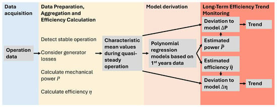
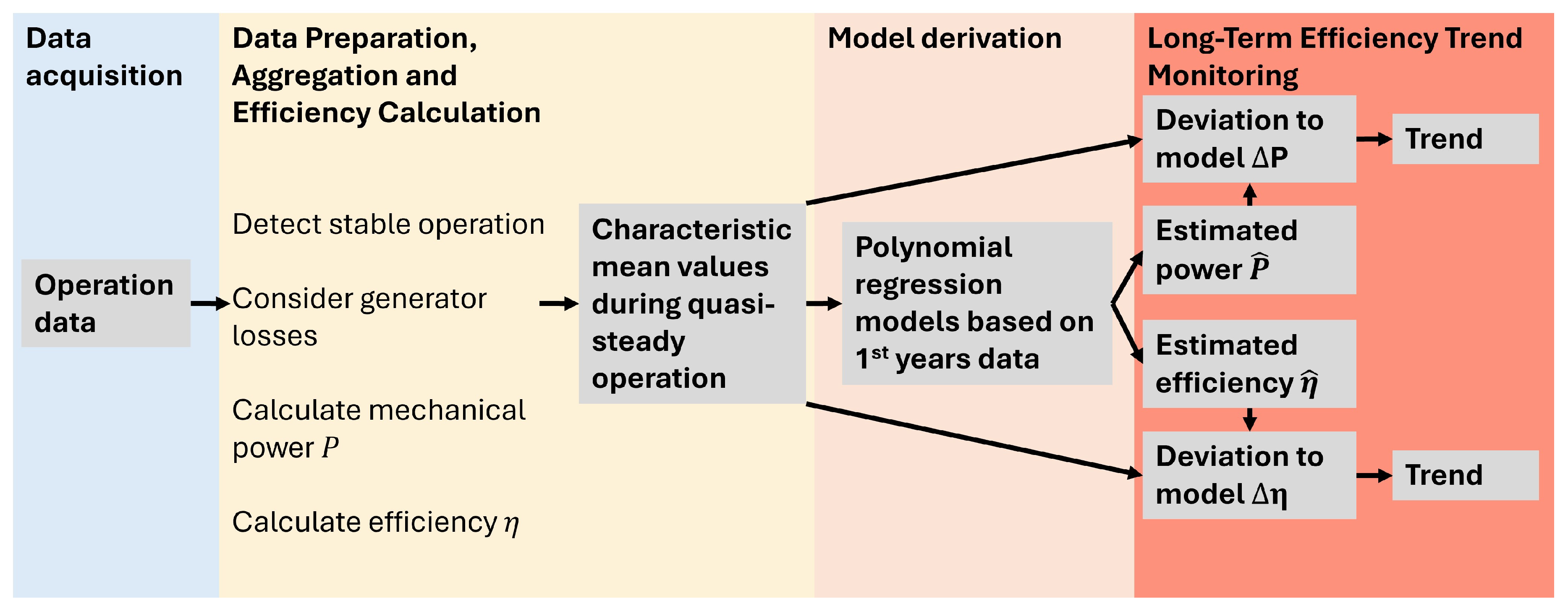
Figure 1 presents the efficiency monitoring workflow, structured into its main process steps.

Figure 1. Efficiency monitoring flowchart.

3.1. Data Preparation, Aggregation and Efficiency Calculation

Prior to efficiency evaluation, the operational data are preprocessed to ensure consistency and comparability during long-term monitoring.

Data preparation delivers mean values of measured signals for periods in which quasi-steady operation was detected. Due to the large amount of data in multi-year considerations, efficient and automated processing, including outlier identification, is necessary.

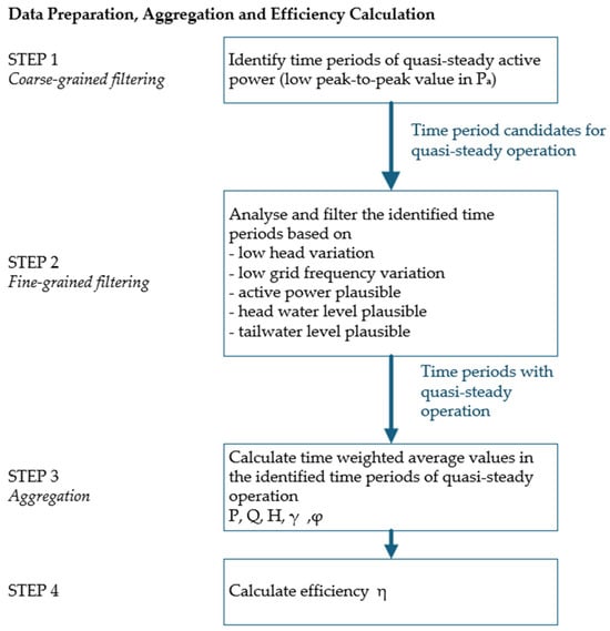
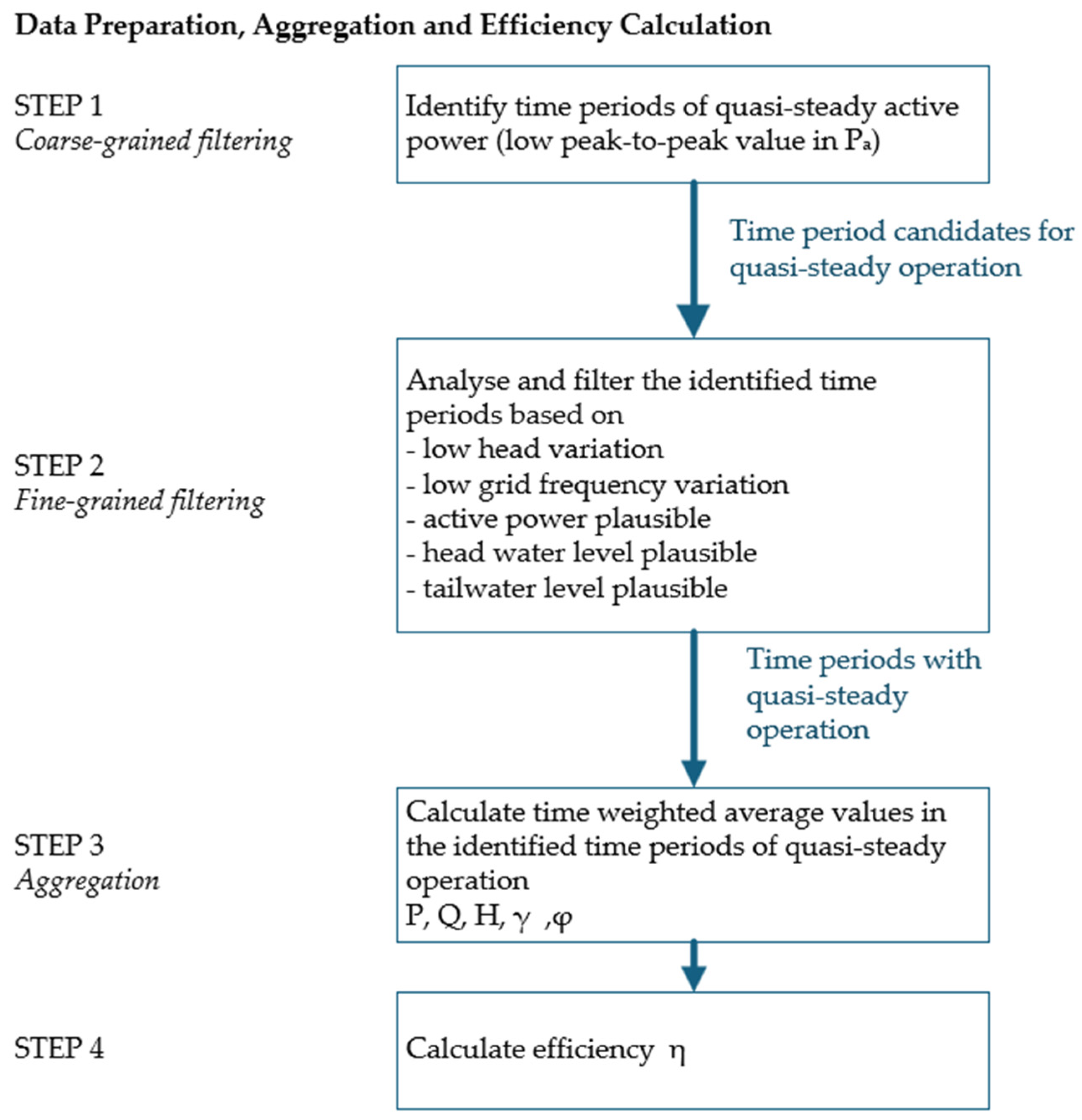
Operational data as measured (so-called raw data) is preprocessed as outlined in Figure 2 to ensure consistency, comparability and under consideration of the basic principles of IEC 60041:1991 [3].

Figure 2. Schematic flowchart of data preparation, aggregation and efficiency calculation.

Application of this International Standard requires consideration of its defined scope and objective: specifying the arrangements for on-site acceptance tests used to assess compliance with contractual guarantees. Accordingly, the present study adopts the underlying principles of the standard and adapts them, where appropriate, to the requirements of long-term performance trending.

Coarse-grained filtering: To ensure reliable and robust long-term efficiency monitoring, only quasi-steady operation is considered. The implemented methodology employs a two-step filtering procedure. In the first step, coarse-grained filtering, time intervals exhibiting low fluctuations in generator power are identified as candidate quasi-steady periods. The parameterization follows [3], which specifies that power variations within the measurement interval should not exceed ±1.5% of the average value.

Fine-grained filtering: In the second step, fine-grained filtering, low fluctuations in grid frequency are verified. Reference [3] specifies that the rotational speed shall not deviate by more than ±0.5% from the average speed. Different rotational speeds result in different stored energy in the rotational masses and a shifted operating point. In addition, only periods during which the head variations are smaller than 0.7% in comparison to the mean head value of that period are considered. Furthermore, periods in which water level measurements yielded implausible values outside the plant-specific typically expected range are excluded. Also, periods containing any electrical-power sample that is negative or exceeds the nominal power are excluded. The duration of the considered periods is 210 s. Accordingly, any period in which at least one sample violates the predefined range or variation criterion is excluded from the subsequent aggregation step.

Aggregation: The losses of the generator P_b vary depending on the reactive load of the generator. Therefore, Ref. [3] suggests that ‘the power factor shall be unity if possible (i.e., cosφ = 1)’. For long-term efficiency monitoring, which must not interfere with power dispatch or grid requirements, such comparable operating conditions are rarely achieved. This greatly limits the number of comparable operating points. Therefore, the mechanical shaft power P was calculated from the measured generator power P_a using the theoretical, manufacturer-provided generator efficiency curves.

For the identified quasi-steady operating periods, time-weighted average values are calculated to compensate for non-equidistant sampling in the operational data. In addition to the averaged values of P, H, and Q, which are required for the subsequent calculation of η, the average guide vane position γ, runner blade position φ, and river water temperature ϑ_water are also determined.

Efficiency calculation: For each previously identified stable operating interval, a single turbine efficiency value is calculated from the corresponding averaged operating point. The efficiency is determined from the mechanical shaft power P, the head H, and the volumetric flow rate Q according to Equation (3). The river water temperature ϑ_water is considered for the density ρ. The calculation of an absolute efficiency value is possible if the physical quantities in Equation (3) are known or measured. In particular, the measurement of discharge Q is not commonly measured in hydropower plants, as accurate measurement systems are relatively expensive and require comparably high installation efforts.

3.2. Determining the Estimated Efficiency

3.2.1. Mathematical Modeling

To estimate unit efficiency and power output, polynomial regression models were employed as a flexible, data-driven approach. A low-order polynomial model function has multiple advantages:

•

Based on characteristic data from a wide range of turbine models and field tests, the turbine efficiency surface as a function of H and Q is expected to be smooth and to exhibit a single dominant maximum over the operating range. A low-order polynomial is well suited to capture the curvature around the best-efficiency point as well as the shift in the optimum with head through interaction terms.

•

The degree of the polynomial and therefore the complexity can be chosen in such a way that the main characteristics of the surfaces of efficiency and power are captured without overfitting to noise in the data. The polynomial degree is determined by observing the RMSE as the polynomial degree is increased. The chosen degree is the lowest degree at which a further increase no longer meaningfully reduces the RSME.

•

Since the model is linear in its coefficients, parameter estimation reduces to a standard linear regression problem with a unique and reproducible solution, avoiding iterative optimization and extensive hyperparameter tuning.

•

The purpose of the model is not to explain the turbine physics in detail but to provide a reliable reference for the current operating point. For this purpose, a smooth model that does not overfit to local anomalies is desirable.

•

In contrast to black-box models, the fitted surface remains transparent and can be visually compared with the manufacturer’s characteristic data from turbine model tests, which is important for establishing plausibility and acceptance in the field.

Two approaches are pursued to estimate the behavior in a given operating point:

•

A flow-dependent estimation of the expected efficiency $\widehat{\eta }$;

•

A flow-independent estimation of the mechanical power P.

3.2.2. Estimation of the Expected Efficiency η

According to Equation (3), the availability of flow measurement data allows the calculation of the absolute efficiency. In the actual model, the target efficiency is therefore expressed as a function of head H and volumetric flow rate Q:

$$\widehat{\eta }=f(H,Q)$$

(4)

As the mechanical power P is linearly dependent on the efficiency, it is excluded from the regression to avoid trivial predictions and to focus on the contribution of H and Q. In the efficiency estimation, the water density ρ is not considered because the temperature dependency of the density has been considered already in the efficiency calculation. The gravitational acceleration g is also excluded, since in the actual context it can be considered as invariant.

3.2.3. Estimation of the Mechanical Power P

Accurate measurement of the volumetric flow rate Q is often challenging and associated with noticeable uncertainty. This is also one of the reasons that such measurements are rarely available in most hydropower plants. To address this issue, it is investigated whether readily available operational parameters can be used as input variables to estimate the expected power output. Specifically, guide vane position γ and, for Kaplan turbines with adjustable runner blades, blade position φ are considered as surrogate inputs. These proxy variables replace the measured flow rate Q in a regression model used to estimate power output P.

With the estimation of the mechanical power P, absolute efficiency cannot be determined directly. However, the change in efficiency δη can be estimated if a corresponding efficiency value from this operating point is known, e.g., from an on-site measurement campaign or characteristic data from turbine tests.

Let

δP = P_t2 − P_t1

(5)

and

δη = η_t2 − η_t1

(6)

where P_t1 corresponds to the absolute efficiency η_t1, for example from a reference measurement, and P_t2 is associated with η_t2 from another measurement. For both measurements, the identical hydraulic operating point is assumed, i.e., Q = constant, H = constant and ρ = constant.

Under these conditions, Equation (3) can be written as

$${\displaystyle \frac{P}{\mathsf{\eta }}}=\rho gQH=\mathit{constant}={\displaystyle \frac{P_{t1}}{{\mathsf{\eta }}_{t1}}}={\displaystyle \frac{P_{t2}}{{\mathsf{\eta }}_{t2}}}$$

(7)

Rearranging Equations (5)–(7) gives

$$\mathrm{\delta }\mathsf{\eta }={\displaystyle \frac{\mathrm{\delta }P}{P_{t1}}}{\mathsf{\eta }}_{t1}.$$

(8)

This means that if a deviating power δP can be determined and the reference power P_t1 and reference efficiency η_t1 are known, the deviating efficiency δη can be calculated.

3.2.4. Training Approaches for Modeling

To determine the most effective training strategy, two alternative approaches for selecting operational data were considered:

• Broad operating range OR-0: Training of the model using most of the available operating points in the dataset, thereby capturing the majority of operating conditions.
• Most frequent operating range OR-1: Training of the model on a relatively narrow operating range that contains the empirical dominant operating region (e.g., the most frequently occurring operating region), thereby focusing on the dominant plant operating condition.

These strategies were analyzed and assessed with respect to whether efficiency or performance can be monitored reliably across the relatively wide operating range in hydropower operation.

At the same time, working within defined operating ranges addresses one of the main limitations of polynomial regression by avoiding unintentional extrapolation beyond the range on which the model was trained.

3.3. Measurement Uncertainty of the Efficiency

Since efficiency is not measured directly but is derived from the measured quantities P, Q, and H, the uncertainties associated with these quantities propagate into the calculated efficiency η. Consequently, an uncertainty analysis is required to quantify the uncertainty of the resulting efficiency values. In this study, the law of propagation of uncertainty is applied, with consideration of Type B uncertainty components [4]. The principal contributors to the uncertainty of η—namely P, Q, and H (see Equation (3))—are examined in detail below, consistent with the measurement principles used in hydraulic turbine field acceptance testing [3].

Type A evaluation of uncertainty was not conducted in the present study because it requires repeated observations under identical measurement conditions, for which the best estimate of the expected value is the arithmetic mean [4]. In this context, identical measurement conditions effectively imply static conditions. However, hydropower turbine operation is generally not static. In the present case, based on a reference power plant in which turbine control is primarily performed in power-control mode (see Section 4.1), the process is inherently dynamic. Permanent micromovements induce, even if only minimally, pressure pulsations, which in turn cause slight flow variations. The conditions identified by our methodology are therefore not strictly static, but only quasi-steady. Any standard deviation of a physical quantity would thus also reflect these fluctuations and would therefore be misleading.

Uncertainty in Power: The electrical power output P_a is determined from measurements of generator terminal currents and voltages using instrumentation such as voltage transformers, current transformers, and power transducers. The combined standard uncertainty $u_{P_a}$ depends on the accuracy of these instruments, as specified by manufacturer data sheets.

Uncertainty in Head: The head H, between the high-pressure measuring section H₁ and low-pressure measuring section H₂, is calculated as

H = H₁ − H₂

(9)

The exact sensor placement should be as close to the turbine as possible. In this study, upstream measurements are taken downstream of the trash rack. Downstream measurements represent the tailwater level. Both head values are measured using pressure sensors, and the pressure values are converted to equivalent distance values. The head at the upstream point H₁, based on the Bernoulli equation for incompressible, frictionless flow, is given by

$$H_1=z_1+{\displaystyle \frac{p_1}{\mathit{\rho g}}}+{\displaystyle \frac{v_1^2}{2g}}$$

(10)

where z₁ is the elevation, p₁ is the pressure, and v₁ = Q/A₁ is the flow velocity, with A₁ the cross-sectional area. A similar expression applies for the head at low-pressure measuring section H₂.

The head is thus

$$H=(z_1-z_2)+{\displaystyle \frac{p_1-p_2}{\mathit{\rho g}}}+{\displaystyle \frac{Q^2}{2g}}\left({\displaystyle \frac{1}{A_1^2}}-{\displaystyle \frac{1}{A_2^2}}\right)$$

(11)

If H₂ is measured at tailwater level, as in our case, the downstream velocity head can be neglected due to low exit velocities, simplifying the equation to

$$H\approx (z_1-z_2)+{\displaystyle \frac{p_1-p_2}{\mathit{\rho g}}}+{\displaystyle \frac{Q^2}{2g{A}_1^2}}$$

(12)

The total uncertainty ∆H in H arises from uncertainties in pressure measurements upstream Δp₁ and downstream Δp₂ and flow rate ∆Q, obtained from sensor specifications, while elevations z₁, z₂, and area A₂ are assumed constant with negligible uncertainty.

Uncertainty in Discharge: The flow rate can be measured using the ultrasonic transit-time technique. The standard uncertainty ∆Q, taken from the device’s specifications, must be accounted for in both Q and its influence on H.

Total Uncertainty in Efficiency: Using Equations (2), (3) and (12), the efficiency is given by

$$\eta ={\displaystyle \frac{P_a}{{\eta }_{\mathit{Gen}}\mathit{\rho gQ}\left[(z_1-z_2)+\frac{p_1-p_2}{\mathit{\rho g}}+\frac{Q^2}{2g{A}_1^2}\right]}}$$

(13)

The combined standard uncertainty u_η is calculated using the law of propagation of uncertainty, assuming the independent variables P_a, Q, p₁ and p₂ are uncorrelated, as

$$u_{\eta }=\sqrt{{\left({\displaystyle \frac{\partial \eta }{\partial P_{\mathit{el}}}}\mathrm{\Delta }{P}_a\right)}^2+{\left({\displaystyle \frac{\partial \eta }{\partial Q}}\mathrm{\Delta }Q\right)}^2+{\left({\displaystyle \frac{\partial \eta }{\partial p_u}}\mathrm{\Delta }{p}_1\right)}^2+{\left({\displaystyle \frac{\partial \eta }{\partial p_d}}\mathrm{\Delta }{p}_2\right)}^2}$$

(14)

with the partial derivatives of η being

$$\begin{array}{l}{\displaystyle \frac{\partial \eta }{\partial P_a}}={\displaystyle \frac{\eta }{P_a}}\\ {\displaystyle \frac{\partial \eta }{\partial Q}}=-{\displaystyle \frac{\eta }{P_h}}\left[\mathit{\rho g}(z_1-z_2)+(p_1-p_2)+{\displaystyle \frac{3\rho Q^2}{2A_1^2}}\right]\\ {\displaystyle \frac{\partial \eta }{\partial p_1}}=-{\displaystyle \frac{\mathit{\eta Q}}{P_h}}\\ {\displaystyle \frac{\partial \eta }{\partial p_2}}={\displaystyle \frac{\mathit{\eta Q}}{P_h}}\end{array}$$

(15)

The combined uncertainty can thus be calculated as

$$u_{\eta }=\eta \sqrt{{\left[\frac{\Delta P_a}{P_a}\right]}^2+{\left[{\displaystyle \frac{\mathit{\rho g}(z_1-z_2)+p_1-p_2+\frac{3\rho Q^2}{2A_1^2}}{P_h}}∆Q\right]}^2+{\left[\frac{Q}{P_h}\right]}^2\left[{∆p_1}^2+{∆p_2}^2\right]}$$

(16)

where P_h = ρgQH. This expression combines the main uncertainty sources that vary with operating conditions.

3.4. Efficiency and Performance Trend Analysis

The efficiency or performance trend is assessed by comparing the actual efficiency η or mechanical power P, computed from the mean values of operational data over each interval of quasi-steady operation, with the estimated efficiency $\widehat{\mathsf{\eta }}$ or estimated mechanical power $\widehat{P}$ predicted by the regression model.

Those comparisons are quantified through the residuals

$$∆\mathsf{\eta }=\mathsf{\eta }-\widehat{\mathsf{\eta }}$$

(17)

$$∆P=P-\widehat{P}.$$

(18)

A residual of zero indicates expected unit performance, while negative values of ∆η or ∆P indicate an efficiency or performance decrease.

4. Results

The developed methodology was validated using a case study of a run-of-river hydropower plant in Northern Europe, commissioned in 2014. The plant comprises two Kaplan turbines, each with a rated power of approximately 50 MW and adjustable runner blades. Each unit has its own penstock where an ultrasonic transit time flow measurement system with four measuring paths from a renowned manufacturer is installed. Operational data have been recorded via a Supervisory Control and Data Acquisition (SCADA) system from July 2020 to September 2026, spanning more than six years, at an approximate sampling rate of 1 Hz.

4.1. Data Preparation, Aggregation and Efficiency Calculation

Data preparation and Aggregation were conducted as described in Section 3.1. This ensured that only representative measurements were aggregated and included. During the first year of data availability, 102,806 candidate intervals satisfying the coarse-grained filtering criteria were identified. Of these, 90,853 intervals with a duration of 210 s passed the fine-grained filtering.

It is worth noting that the turbine was primarily operated in power-control mode. In this mode, the operator provides power setpoints to the control loop, while the guide vane position γ is adjusted by the controller. Consequently, small continuous movements of the guide vane regulating mechanism occur. Measurements according to IEC 60041:1991 [3] are usually conducted in opening-control mode, which typically provides more stable conditions. However, since long-term efficiency monitoring must not interfere with operation or grid requirements, power-control mode must be accepted, although opening-control mode would be preferable from a measurement and analysis perspective.

The efficiency η is calculated based on characteristic mean values during quasi-steady periods, with the temperature dependence of water density taken into account.

4.2. Determining the Estimated Efficiency

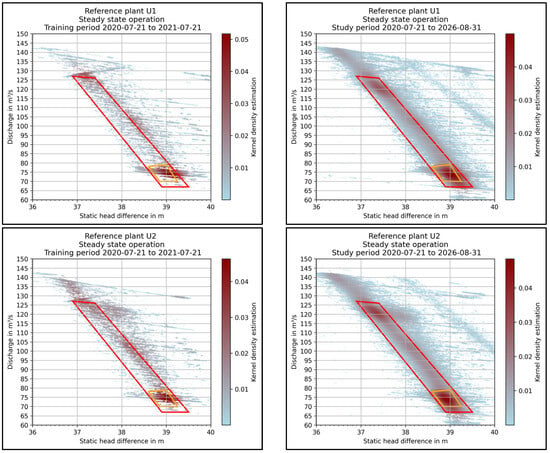
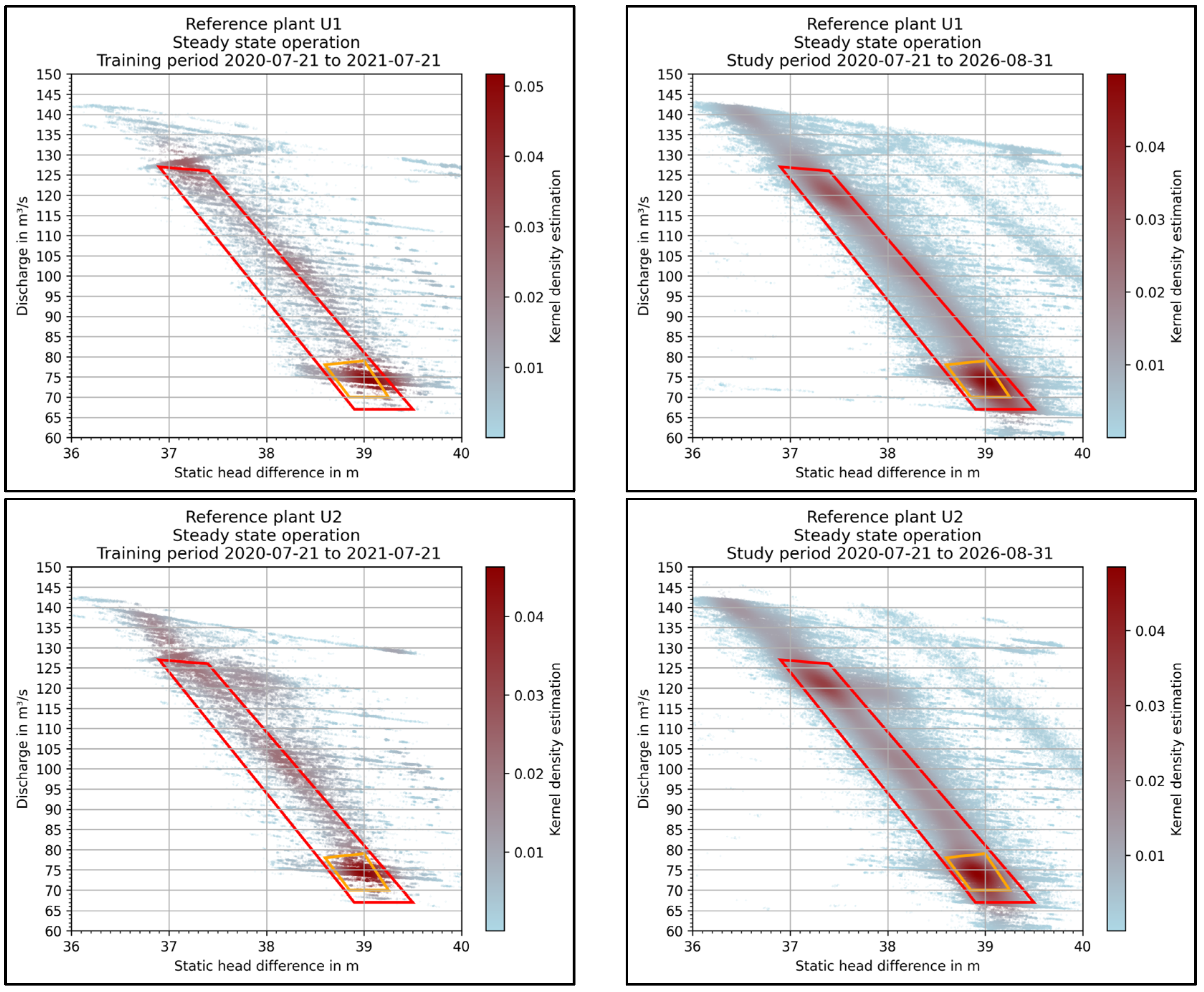
Figure 3 illustrates the distribution of quasi-steady operating points in the H–Q diagram. The kernel density estimate highlights the most frequented regions of operation and provides a representation of the units’ operating scheme. The upper panels correspond to power unit 1 of the reference power plant, and the lower panels to power unit 2. The panels on the left show the first year of data availability (21 July 2020 to 21 July 2021), which was used as the training period for the multivariate regression model. The panels on the right show the full study period, including all available data.

Figure 3. Distribution of quasi-steady operating points for the two examined power units (top unit 1, bottom unit 2) of the reference power plant. Left: training period. Right: entire study period. Red trapezoid: broad operating range (OR-0). Orange trapezoid: most frequent operating range (OR-1).

For comparability, OR-0 and OR-1 were defined identically for both power units, with the boundaries primarily based on the long-term operating scheme of unit 2.

The training period was chosen to span one calendar year in order to capture and balance seasonal effects on performance or efficiency.

Based on the defined operating ranges and the selected training period, the following set of polynomial regression models was derived for both units and both operating ranges:

• Estimation of efficiency $\widehat{\mathsf{\eta }}$, based on the operating point identified in the H-Q-domain.
• Estimation of mechanical power $\widehat{P}$, based on the operating point identified in the H_static-Q-domain using the static head difference.
• Estimation of mechanical power $\widehat{P}$, based on the operating point identified in the H_static-γ-domain using the static head difference.

For the guide vane position γ-based models, the static head H_static was selected as an input variable to obtain a flow-independent model. For consistency and ease of comparison H_static was used for all power estimation models.

To evaluate the model fit, 20% of the data from the training period was reserved for testing. This subset was used to calculate the test RMSE and test R², and was not used for training purposes. Table 1 and Table 2 contain the model performance metrics. The bold figures indicate the selected polynomial degree.

Table 1. Performance metrics of the efficiency estimation models for the two power units and considered operating ranges (dimensionless). Values without brackets are from the validation split; values in brackets from the training split. The selected polynomial degree is indicated in bold.

		Feature Variables/Unit/Operating Range
Polynomial Degree		H, Q/ U1/ OR-0	H, Q/ U2/ OR-0	H, Q/ U1/ OR-1	H, Q/ U2/ OR-1
1	Test RMSE	0.002321	0.002152	0.001786	0.001626
	Test R2	0.7201	0.6659	0.0545	0.0813
	Train RMSE	0.002346	0.002130	0.001765	0.001612
2	Test RMSE	0.001694	0.001492	0.001783	0.001621
	Test R2	0.8509	0.8393	0.0582	0.0866
	Train RMSE	0.001685	0.001470	0.001764	0.001595)
3	Test RMSE	0.001694	0.001489	0.001782	0.001619
	Test R2	0.8510	0.8400	0.0587	0.0892
	Train RMSE	0.001684	0.001466	0.001763	0.001593
4	Test RMSE	0.001692	0.001485	0.001763	0.001619
	Test R2	0.8512	0.8409	0.0791	0.0892
	Train RMSE	0.001681	0.001460	0.001746	0.001591
5	Test RMSE	0.001692	0.001484	0.001765	0.001621
	Test R2	0.8512	0.8410	0.0773	0.0873
	Train RMSE	0.001680	0.001459	0.001746	0.001587
6	Test RMSE	0.001687	0.001472	0.001770	0.001621
	Test R2	0.8521	0.8436	0.0724	0.0870
	Train RMSE	0.001677	0.001449	0.001742	0.001586
7	Test RMSE	0.001682	0.001472	0.001770	0.001621
	Test R2	0.8530	0.8436	0.0721	0.0869
	Train RMSE	0.001672	0.001448	0.001742	0.001586
8	Test RMSE	0.001679	0.001471	0.001770	0.001621
	Test R2	0.8535	0.8437	0.0718	0.0864
	Train RMSE	0.001670	0.001448	0.001742	0.001588
9	Test RMSE	0.001680	0.001472	0.001770	0.001621
	Test R2	0.8534	0.8436	0.0717	0.0863
	Train RMSE	0.001670	0.001448	0.001741	0.001587

Table 2. Performance metrics of the power estimation models for the two power units and defined operating ranges. RMSE values are expressed in MW. Bold values denote the selected polynomial degree of the implemented model.

		Feature Variables/Unit/Operating Range
Polynomial Degree		Hstatic, Q/U1/ OR-0	Hstatic, Q/U2/ OR-0	Hstatic, Q/U1/ OR-1	Hstatic, Q/U2/ OR-1	Hstatic, γ/U1/ OR-0	Hstatic, γ/U2/ OR-0	Hstatic, γ/U1/ OR-1	Hstatic, γ/U2/ OR-1
1	Test RMSE	0.111758	0.106917	0.049455	0.045479	0.126104	0.112814	0.079426	0.076385
	Test R2	0.9997	0.9997	0.9854	0.9891	0.9996	0.9997	0.9622	0.9698
	Train RMSE	0.109499	0.108287	0.049317	0.045037	0.125516	0.113121	0.078831	0.077235
2	Test RMSE	0.056216	0.049403	0.049332	0.045211	0.114117	0.102922	0.079569	0.076209
	Test R2	0.9999	0.9999	0.9854	0.9892	0.9996	0.9997	0.9621	0.9700
	Train RMSE	0.055583	0.049091	0.049241	0.044631	0.113345	0.103188	0.078480	0.077119
3	Test RMSE	0.055875	0.049328	0.049286	0.045150	0.101363	0.090237	0.078901	0.075314
	Test R2	0.9999	0.9999	0.9855	0.9892	0.9997	0.9998	0.9627	0.9707
	Train RMSE	0.055268	0.048932	0.049229	0.044611	0.100061	0.090062	0.077901	0.076238
4	Test RMSE	0.055786	0.049202	0.048808	0.045103	0.101000	0.089577	0.078204	0.074951
	Test R2	0.9999	0.9999	0.9857	0.9893	0.9997	0.9998	0.9634	0.9709
	Train RMSE	0.055129	0.048794	0.048789	0.044584	0.099636	0.089230	0.077215	0.075860
5	Test RMSE	0.055797	0.049185	0.048782	0.045048	0.095470	0.085347	0.077810	0.073747
	Test R2	0.9999	0.9999	0.9858	0.9893	0.9998	0.9998	0.9637	0.9719
	Train RMSE	0.055078	0.048784	0.048783	0.044463	0.094894	0.084954	0.076616	0.075181
6	Test RMSE	0.055701	0.048790	0.048738	0.044971	0.094382	0.084233	0.077770	0.073545
	Test R2	0.9999	0.9999	0.9858	0.9893	0.9998	0.9998	0.9638	0.9720
	Train RMSE	0.054950	0.04841	0.048728	0.044434	0.093743	0.083884	0.076418	0.074955
7	Test RMSE	0.055605	0.048789	0.048735	0.044972	0.093445	0.083364	0.077773	0.073548
	Test R2	0.9999	0.9999	0.9858	0.9893	0.9998	0.9998	0.9638	0.9720
	Train RMSE	0.054881	0.048408	0.048726	0.044434	0.093031	0.082915	0.076424	0.074968
8	Test RMSE	0.055552	0.048791	0.048729	0.045005	0.093343	0.083222	0.077775	0.073550
	Test R2	0.9999	0.9999	0.9856	0.9893	0.9998	0.9998	0.9638	0.9720
	Train RMSE	0.054823	0.048403	0.048720	0.044497	0.092889	0.082724	0.076430	0.074982
9	Test RMSE	0.055561	0.048792	0.048721	0.044991	0.093342	0.083248	0.077777	0.073554
	Test R2	0.9999	0.9999	0.9856	0.9893	0.9998	0.9998	0.9638	0.9720
	Train RMSE	0.054835	0.048407	0.048711	0.044483	0.092891	0.082743	0.076436	0.074996

To justify the selected polynomial degrees of the implemented models, the RMSE obtained on the training data was primarily considered. Lower values indicate a better model fit. In general, the polynomial degree was chosen as a compromise between model complexity and predictive accuracy, such that a higher degree was only selected when it led to a meaningful improvement in the performance metrics.

For the efficiency estimation $\widehat{\mathsf{\eta }}$, based on the operating point identified in the H-Q-domain, the test RMSE ranged from 1.490‰ to 1.746‰ for the selected fourth-degree polynomial. Training and test RMSE values were comparable, indicating that the models generalize with an error level similar to that observed during training. The fourth-degree polynomials were selected for U2 because a higher polynomial degree did not improve the performance metrics significantly. For U1, the test RMSE even decreased for the fifth-degree polynomial, suggesting overfitting. The relatively low coefficient of determination R² obtained for OR-1 must be interpreted in light of the limited dispersion of the target variable η. For U2 OR-1, the total sum of squares (SST) was 0.006348, and the sum of squared errors (SSE) was 0.005782, yielding an R² value of 0.0892 according to R² = 1 − SSE/SST. The standard deviation of the OR-1 target variable η was 0.001697, indicating a narrow spread of the data. Although the RMSE remained small in absolute terms (0.001619), this error constitutes a substantial proportion of the inherent variability in the OR-1 response. As a result, the model accounts for only a limited fraction of the variance in this subset. Therefore, the low R² observed for OR-1 reflects the restricted dynamic range of the target variable rather than necessarily indicating poor absolute predictive performance.

For the mechanical power estimation $\widehat{P}$, based on the operating point identified in the H-Q-domain using the static head difference, the RMSE ranged from 0.0451 MW to 0.0558 MW for the selected fourth-order polynomial. Training and test RMSE values were comparable, indicating that the models generalize with an error level similar to that observed during training.

When the operating point is identified using the static head difference H_static and the guide vane opening γ, the RMSE for estimation ranged from 0.0737 MW to 0.0934 MW. For example, for OR-1, where the mechanical power is typically in the range of 25–28 MW, an RMSE of 0.0737 MW corresponds to a relative error of approximately 0.28% (0.0737 MW/26.5 MW).

For the mechanical power estimation $\widehat{P}$, we observed a better model fit for the narrower operating range OR-1 than for the broader operating range OR-0. This is consistent with the fact that OR-1 covers a smaller range of operating conditions than OR-0. In addition, U2 generally showed a better model fit than U1. This is consistent with the fact that the selected operating range was primarily based on the long-term operating data of U2.

4.3. Measurement Uncertainty of the Efficiency η

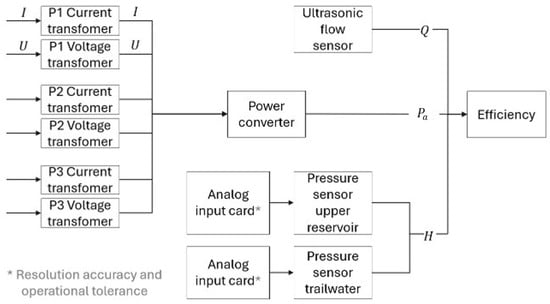
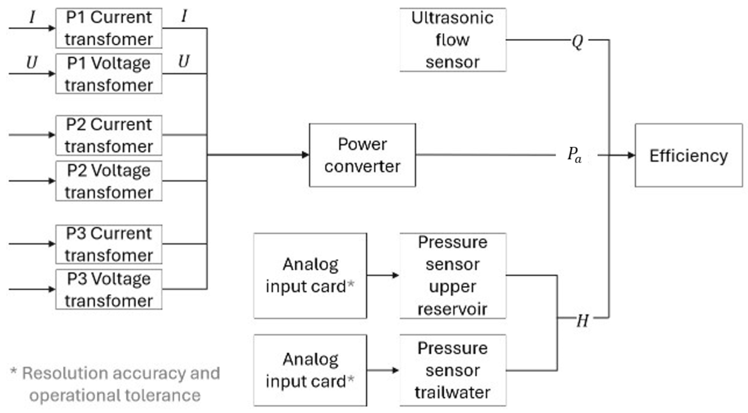
To enable comparison with the measured data, this section presents the measurement uncertainty estimation for the hydropower plant. The measurement chain can be seen in Figure 4.

Figure 4. Measurement chain of the used instrumentation.

In this study, we used type B uncertainties from manufacturer specifications, as shown in Table A1, listing the relevant measurement instrumentation, the stated uncertainty, and its type (e.g., standard deviation or maximum error). When a maximum error was provided, the value specified by the manufacturer was interpreted in this study according to Section 4.3.7 in ref. [4] which assumes a rectangular probability distribution. In this case, the standard uncertainty u is calculated as

$$u={\displaystyle \frac{\left|a\right|}{\sqrt{3}}}$$

(19)

where a is the maximum deviation from the true value, as specified in the manufacturer’s data sheet. This conversion ensures consistency with standard uncertainty propagation practices. Throughout this work, the expanded uncertainty with a coverage factor k = 2 according to [4] is used. This corresponds approximately to a 95% coverage probability under the stated assumptions.

To evaluate the total uncertainty in efficiency, the relevant standard measurement uncertainty of the components in the measuring chain is quantified; see Equation (14).

Uncertainty in discharge Q: The derived standard deviation is based on the manufacturer’s specified uncertainty of ±1.155%.

Uncertainty in pressure difference ∆p: This arises from the used equipment—in this case, the pressure sensor and the analog input card with the resolution accuracy and the operational tolerance. It is identical for p₁ and p₂, as the same instrumentation is used and can be calculated as

$$\Delta p=\pm \sqrt{{(0.37\%)}^2+{(0.00087\%)}^2+{(0.058\%)}^2}\cdot p=\pm 0.3745\%\cdot p$$

(20)

Uncertainty in the generator power P_a: This results from the uncertainties of the current and voltage transformers P_tf as well as the power transducer P_td:

$${\displaystyle \frac{\Delta P_a}{P_a}}=\sqrt{{\left(\frac{\Delta P_{\mathrm{tf}}}{P_a}\right)}^2+{\left(\frac{\Delta P_{\mathrm{td}}}{P_a}\right)}^2}.$$

(21)

For a three-phase system with balanced load, the total power is given by

$$P_{\mathrm{a}}=\sqrt{3}\mathit{U}I\cos {\phi }_{\mathit{el}}$$

(22)

where U and I denote the voltage and current, respectively, and φ_el is the angular difference between the voltage and the current. The phase shift uncertainty was neglected, as the phase angle is small under normal conditions and the cosine function varies minimally near zero, making its impact on power calculation negligible.

The relative uncertainty of the transformer measurements is

$${\displaystyle \frac{\Delta P_{\mathrm{tf}}}{P_a}}=\sqrt{{\left(\frac{\Delta U}{U}\right)}^2+{\left(\frac{\Delta I}{I}\right)}^2}=0.1626\%$$

(23)

where ΔU/U = ΔI/I = ± 0.115%. The uncertainty of the power transducer is

$${\displaystyle \frac{\Delta P_{\mathrm{td}}}{P_a}}=0.289\%$$

(24)

The total uncertainty of the power measurement is then calculated as

$$\Delta P_a=\pm \sqrt{\Delta P_{\mathrm{tf}}^2+\Delta P_{\mathrm{td}}^2}=\pm 0.3316\%\cdot P_a$$

(25)

Total Uncertainty in the Efficiency η: The overall uncertainty in efficiency u_η is calculated using Equation (16) with the input values above, to consider the operating point, which yields the following formula

$$u_{\eta }=\eta \sqrt{{\left[0.3316\%\right]}^2+{\left[{\displaystyle \frac{\mathit{\rho g}(z_1-z_2)+p_1-p_2+\frac{3\rho Q^2}{2A_1^2}}{P_h}}\cdot 1.155\%\cdot Q\right]}^2+{\left[0.3745\%{\displaystyle \frac{Q}{P_h}}\right]}^2\left[p_1^2+p_2^2\right]}$$

(26)

The boundary points of the trapezoidal operating range OR-0 in the HQ-diagram are selected to illustrate the uncertainty values: the maximum and minimum head H at the highest and lowest flow rate Q. For each of the four operating points, the standard uncertainty u_η (68% level of confidence) and the expanded uncertainty U_η = 2u_η (approximately 95% level of confidence) were calculated. The standard uncertainty provides an estimate of the typical variation expected in repeated measurements, whereas the expanded uncertainty indicates the interval within which the true value is likely to lie with a higher level of confidence. Both are considered to provide a more comprehensive assessment of measurement reliability. As shown in Table 3, the standard uncertainties range from ±1.086%pt to ±1.123%pt, while the expanded uncertainties range from ±2.172%pt to ±2.246%pt for the four representative operating points.

Table 3. Measurement uncertainty of the efficiency at the boundary points of the operating range OR-0 as mean values during the training period of U2.

OR-0	Hmin, Qmin	Hmin, Qmax	Hmax, Qmax	Hmax, Qmin
Efficiency η	91.40%	92.21%	92.31%	91.75%
Standard uncertainty uη	1.086%pt	1.123%pt	1.122%pt	1.092%pt
Expanded uncertainty Uη	2.172%pt	2.246%pt	2.244%pt	2.184%pt

4.4. Efficiency and Performance Trend Analysis

4.4.1. Trend Analysis for U1 of the Reference Power Plant

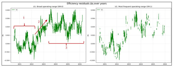
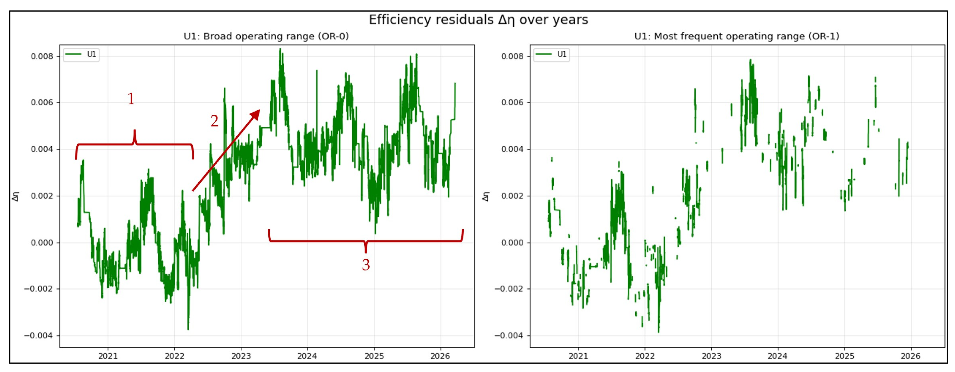
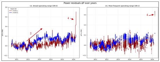
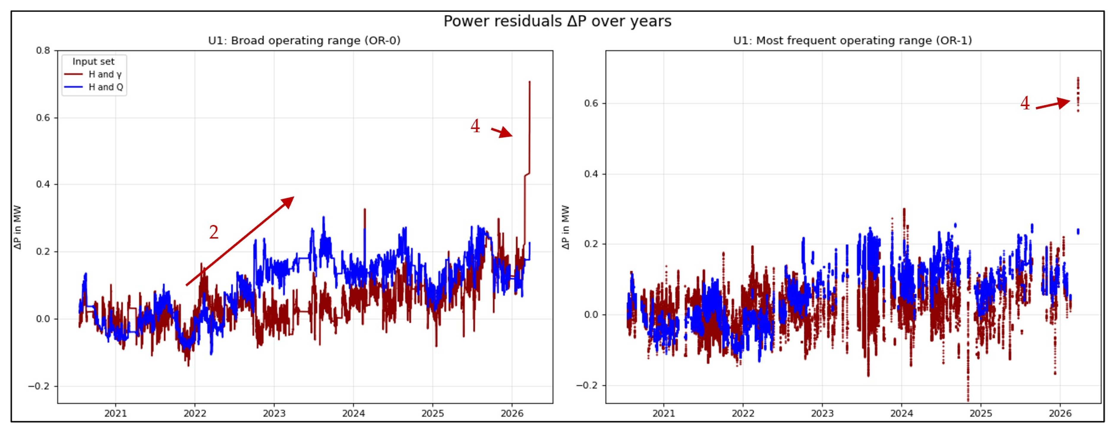
Figure 5 shows the multi-year trend of the efficiency residuals Δη for reference unit 1, i.e., the deviation of the actual efficiency η from the regression model OR-0 and 1. Figure 6 illustrates the multi-year trend of the power residuals ΔP for reference unit 1, i.e., the deviation of the actual efficiency η from the regression model OR-0 and OR-1. The following observations can be made about the two figures. The models were fitted to data from 20 July 2020 to 20 July 2021. A rolling mean with a window size of 200 samples was applied, as the present study focuses on long-term trends. As noted in Section 3.1, after mean aggregation, each quasi-steady period has a fixed duration of 210 s. Because the 200-sample mean is specific to the operating range, and the power unit may operate for an unpredictable duration outside this range, a time-based rolling mean would only produce values once 200 samples are available within the respective time window. In particular, this would reduce the number of data points for OR-1 in the diagram. Since the objective of this study is to capture long-term trends, a sample-based rolling mean was therefore chosen.

Figure 5. Efficiency residual ∆η over time in the broad operating range OR-0 (right) and in the most frequented operating range OR-1 (left) for reference unit 1.

Figure 6. Power residual ∆P over time in the broad operating range OR-0 (left) and in the most frequented operating range OR-1 (right) for reference unit 1.

The following observations can be made.

• From June 2020 to April 2023, the trend remains relatively stable. Except for two peaks, Δη stays within ±3‰, which is well within the expanded uncertainty U_η. Similar to unit 2, we observe—despite temperature compensation for water density—a seasonal pattern in the efficiency, with the highest efficiency occurring around August and the lowest at the beginning of the calendar year. This is remarkable as the higher water density at lower temperature is expected to yield more power; see Equation (7). A possible explanation is an uncompensated temperature-dependent bias in the water-level measurements. In the vertical measurement pipes, piezoelectric pressure transducers are installed below the water surface and suspended by relatively long wire-mesh-reinforced polyurethane cables. At the upper end of each measuring pipe, the cable is fixed with a clamping device. The same principle is used for both the tailrace and headwater level measurements, although with different cable lengths. Therefore, the thermal expansion of the cable of the tailrace water-level probe may show higher values, causing the measured head to decrease at higher water temperatures. This would result in an apparent seasonal increase in efficiency during the warmer period of the year.
• In period 2, a gradual improvement in efficiency is observed. However, this improvement is not reflected in a rising power residual resulting from the power prediction of the H-γ-model. Therefore, it is concluded that a drift in the flow measurement has occurred during that period. A consultation with the plant owner after conducting the analytics of this study supports this conclusion. A warning for one ultrasonic measuring path occurred before autumn 2025. The exact date was not logged. However, in line with the findings of this study, it is likely to have occurred in period 2.
• After the flow-meter fault as per point 2, the efficiency residual fluctuated slightly around approximately 5‰, in with a variation between 1‰ and 8, the overall trend does not indicate an efficiency degradation.
• Like U2, in spring 2026, the cam curve was modified to improve vibrational behavior rather than to optimize efficiency. The observed step change is caused by the resulting mismatch with the original base model. This retrospective interpretation is based on the information provided by the plant owner after conducting the analytics of this study. A new model derivation is therefore required in the future to account for this change.

4.4.2. Trend Analysis for U2 of the Reference Power Plant

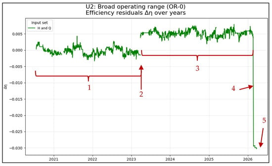
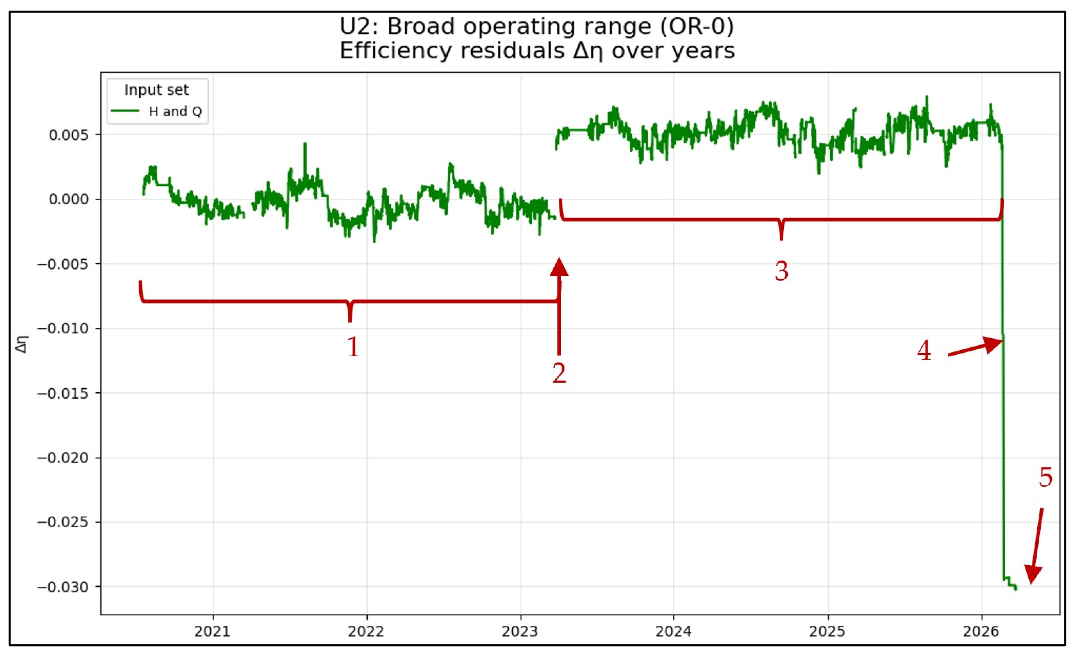
Figure 7 shows the multi-year trend of the efficiency residuals Δη for reference unit 2, i.e., the deviation of the actual efficiency η from the regression model OR-0, which was fitted to data from 20 July 2020 to 20 July 2021. A rolling mean with a window of 200 samples was applied because the focus of this study is on long-term trends, while short-term fluctuations are considered negligible. The following observations can be made.

Figure 7. Efficiency residual ∆η over time in the broad operating range OR-0 for reference unit 2.

• From June 2020 to April 2023, the trend remains relatively stable. Except for two isolated peaks, Δη stays within ±3‰, which is well within the expanded uncertainty U_η. Despite temperature compensation for water density, a seasonal pattern is still visible in the efficiency, with the highest efficiency occurring around August and the lowest at the beginning of the calendar year.
• Between periods 1 and 3, an apparent and sudden improvement (jump) in efficiency is observed. However, consultation with the plant operator revealed that a flow-meter fault was detected on 2 April 2023, most likely caused by a malfunction in one of the four ultrasonic measuring paths.
• After the revealed flow-meter fault in April 2023, as per point 2, the efficiency residual variation is comparable to the period prior to point 2 but with fluctuations now in the range from +2‰ to +7.5‰.
• Also, similar to the discussion of Figure 6, a flow-meter fault is likely to be observed and justified.
• As noted at the beginning of Section 4, operational data are available from July 2020 to September 2026. However, no efficiency residuals were calculated after 25 March 2026, because after that date the tailwater level at the plant was lowered by approximately 2 m. This led to a head increase, which is not covered by the predefined operating ranges OR-0 and OR-1. Thus, there exists no valid model for that operating range.

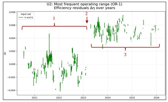
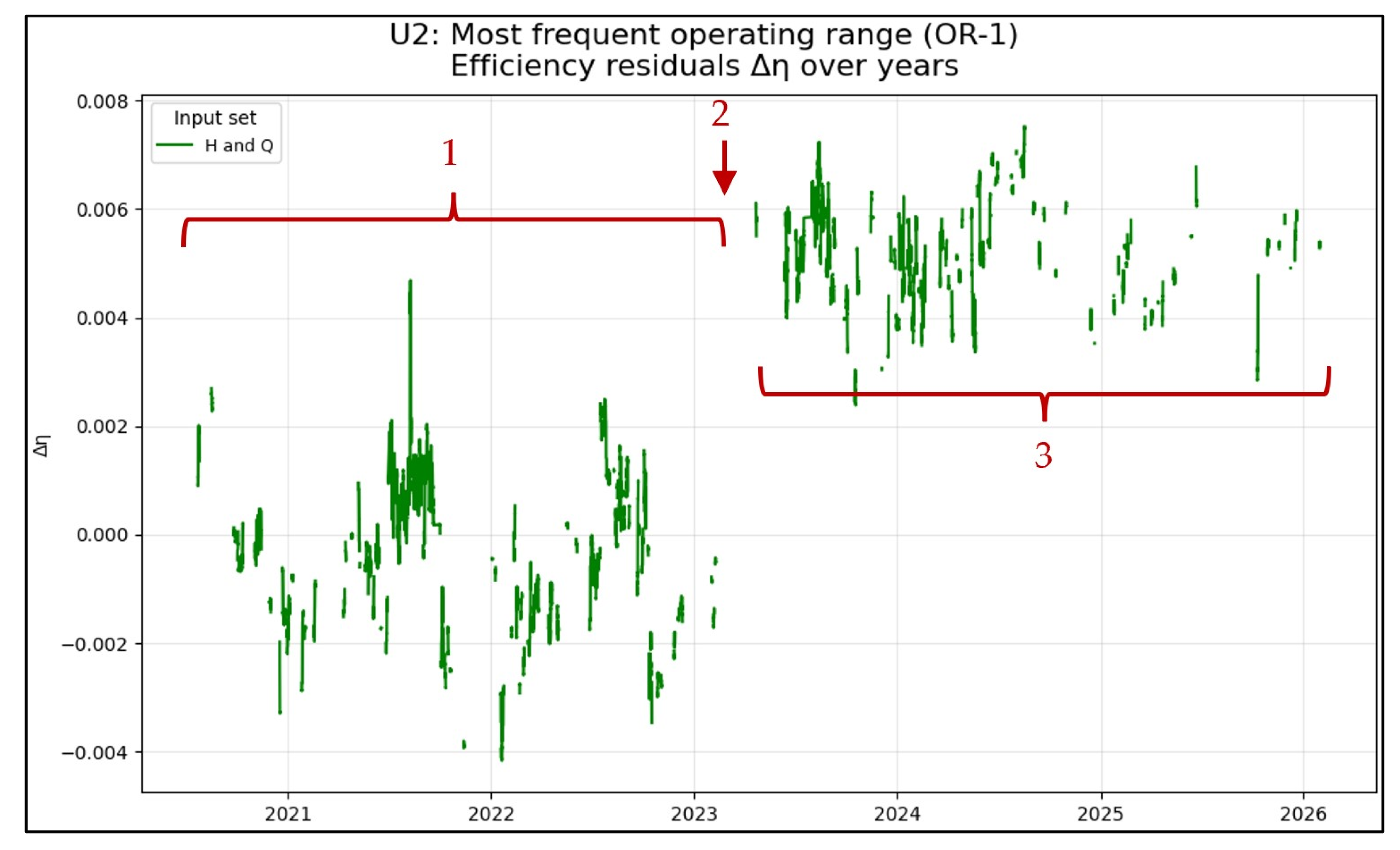
Figure 8 shows the multi-year trend of the efficiency residuals Δη for reference unit 2, i.e., the deviation of the actual efficiency η from the regression model OR-1. As for OR-0, a rolling mean with a window of 200 samples was applied.

Figure 8. Efficiency residual ∆η over time in the most frequented operating range OR-1 for reference unit 2.

The observations are congruent with those of OR-0.

• From June 2020 to April 2023, the trend shows fluctuations, but an overall decreasing trend cannot be deduced. Also, a seasonal pattern is observable here. Except for the isolated peak in August 2021, Δη stays within a range of approximately +2.5‰ to −4‰, which is again well within the calculated expanded uncertainty U_η.
• Between periods 1 and 3, also an apparent improvement in efficiency is observed. As described above, this falls in line with a failure indication of the flow-meter reported by the plant owner after conducting the analytics of the study.
• After the revealed flow-meter fault in April 2023, as per point 2, the efficiency residual fluctuated slightly around approximately +5‰, in the range from +2.5‰ to +7.5‰.

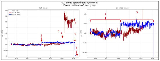
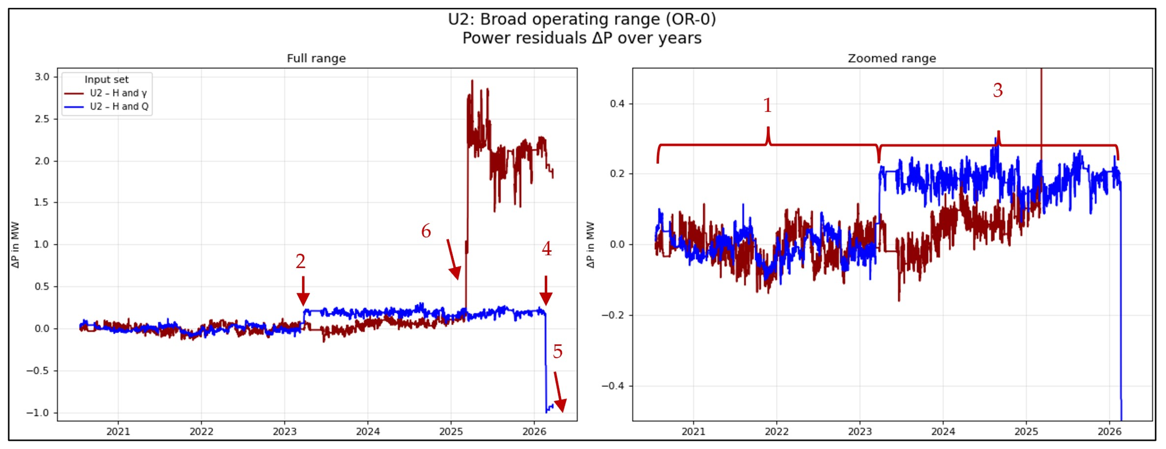
Figure 9 shows the multi-year evolution of the power residuals ΔP for reference unit 2, i.e., the deviation of the actual power P from the regression model OR-0 fitted to data from 20 July 2020 to 20 July 2021. A rolling mean with a window length of 200 samples was applied. The following observations can be made.

Figure 9. Power residual ∆P over time in the broad operating range OR-0 for reference unit 2. The left panel shows the full range. The right panel shows the zoomed range.

• From June 2020 to April 2023, both residual trends remained relatively stable. The residuals based on H and Q exhibit smaller fluctuations than those based on H and γ. Moreover, no seasonal pattern is apparent in the residuals based on H and γ. Overall, no degradation in performance is visible during this period.
• When the previously mentioned flow-meter fault occurred, the residual trend based on H and γ remained essentially unchanged, supporting the hypothesis of a fault in the flow-meter path. In contrast, only the residual based on H and Q showed a step change.
• During Period 3, the residual based on the H-Q-model remained stable. The residual based on the H-γ-model, however, indicates a slight apparent performance improvement. Since such an improvement is unlikely and is not reflected in the efficiency analysis, we assume a minor change in the guide-vane regulating mechanism or drift in the position measurement. A drift in head measurement would also affect the power and efficiency estimates based on H and Q, which is not observed in any other figure. The trend suggests that a slightly smaller guide-vane opening is required to achieve the power predicted by the model.
• Again, the power estimated from flow rate and head exhibits a step change. In contrast to point 2, this step indicates a significant loss in performance. No step of comparable magnitude is observed in the residuals of the power estimate based on H and γ. This further suggests the presence of an additional flow-meter fault as the most likely explanation.
• As noted above, operational data are available until September 2026; however, due to a lowering of the tailwater level, the operating point left the valid model range, and residuals are therefore not evaluated beyond this point.
• In March 2025, the cam curve was modified to improve vibrational behavior rather than optimize efficiency. The observed step change is caused by the resulting mismatch with the original base model. A new model derivation is therefore required to account for this change.

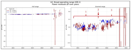
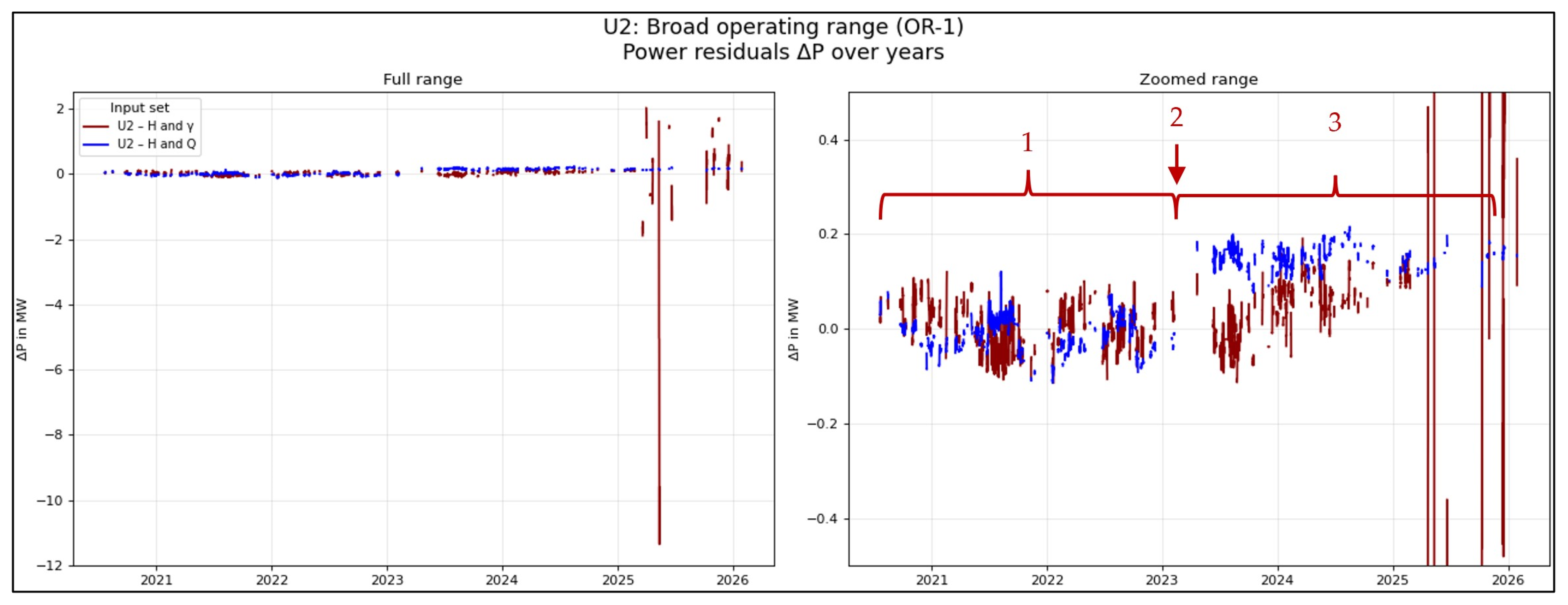
Figure 10 shows the multi-year evolution of the power residuals ΔP for reference unit 2, i.e., the deviation of the actual power P from the regression model OR-1 fitted to data from 20 July 2020 to 20 July 2021. A rolling mean with a window length of 200 samples was applied. The findings described in detail in Figure 9 can be seen here as well.

Figure 10. Power residual ∆P over time in the most frequent operating range OR-1 for reference unit 2. The left panel shows the full range. The right panel shows the zoomed range.

4.5. Discussion of the Results

This study investigates long-term monitoring of hydropower plant efficiency, with respect to model development, measurement uncertainty, and practical implementation challenges.

The main findings can be summarized as follows:

•

A conceptual framework for efficiency trend monitoring was developed. Long-term monitoring of efficiency trends is feasible by tracking the residuals between the predicted estimated efficiency and actual measured efficiency (calculated based on the current operating point). With data from a four-path ultrasonic transit-time flow-meter, a thorough identification of quasi-steady conditions, consideration of generator losses, and automated outlier handling were performed; the obtained results are well within the expected measurement uncertainty. Trends showed variation in the per mill range of the efficiency, where even seasonal influences could be observed.

•

However, despite this achieved order of magnitude in the trends, it is necessary to assess whether the observed patterns are genuinely meaningful or potentially misleading. Therefore, a second proxy variable for the flow, such as guide vane opening γ is necessary to verify the results obtained. In our study, three occurrences of deviating discharge metering could be identified.

•

Hydropower efficiency can be accurately modeled using polynomial regression incorporating head H and discharge Q as input variables.

•

Performance trending, in the absence of a direct flow measurement, is possible. In our case study, the power, serving as a performance indicator, was estimated based on the guide vane opening γ and static head H. These are measurement quantities that are available in practically all hydropower plants. In the case of a Kaplan turbine, where the discharge is not solely dependent on the guide vane position, but also on the runner blade position φ, trending yielded reasonable results as long as the cam curve remained unchanged.

5. Conclusions and Outlooks

This study demonstrates that long-term monitoring of hydropower turbine efficiency can be performed using ultrasonic transit-time flow measurements. It became evident that in addition to comparing the actual efficiency—defined at specific operating points—with efficiency estimates derived from characteristic performance data, a second validation criterion is beneficial to improve the robustness and significance of the results. In this study, guide vane opening γ is used for this purpose. After evaluation, the long-term efficiency trend observed does not show a significant efficiency degradation; the fluctuations remain in the per mill range and are well within the estimated measurement uncertainty. It is further concluded that, in plants where direct flow measurements are not available, guide vane opening combined with a reliable static head measurement can be used as an input variable to a mathematical model for estimating the expected output power. For the Kaplan turbine investigated in this study, this approach proved effective as long as the cam curve, i.e., the correlation between runner blade and guide vane position, remained unchanged. Any adaptation of the cam curve requires reestablishing the underlying base model.

The limitations identified in this study suggest the following directions for future research:

•

The results showed a systematic annual pattern, for which a possible cause was identified as an uncompensated temperature bias in the level measurement. However, the available data alone do not provide sufficient evidence to confirm this hypothesis. Further investigation of this phenomenon is recommended. Until the cause is clarified, trend interpretation should be based on expert judgment, and comparisons should be made only at similar seasonal time points. In addition, the scatter may potentially be reduced by applying improved trend estimation, for example by using an extended sampling window or a regression-based polynomial trend line.

•

Validate the approach using longer datasets from a wider range of plants and turbine types. Also, the efficiency or performance in the pumping mode of pump turbines or pumps of ternary pumped storage sets could be analyzed, in this case the pump head should correlate with the power consumption, means guide vane opening is not a valid input variable since the guide vane opening is adapted in order to optimize pump efficiency by improving pump exit flow conditions (second order effect) rather than controlling the discharge itself as in turbine mode (first order effect); therefore any degradation of the pump itself needs to be handled independently from the optimal guide vane setting—in some sense this is comparable to the cam curve optimization in double-regulated machines, where the best blade tilt can also be regarded as a second order effect to the general turbine performance.

•

Assess the limitation of the calibrated operating range, since the proposed regression models are valid only within the range covered by the training data. Operation outside this range is currently not considered in the evaluation.

•

Investigate advanced modeling approaches, such as deep learning or physics-informed methods, to improve the fitness of the model.

•

Correlate efficiency estimation results with power output estimation to develop a consistency indicator.

References

- International Hydropower Association (IHA). 2026 World Hydropower Outlook; IHA: London, UK, 2026; p. 24. Available online: https://www.hydropower.org/publications/2026-world-hydropower-outlook (accessed on 30 September 2026).
- Kashyap, T.; Thakur, R.; Ngo, G.; Lee, D.; Fekete, G.; Kumar, R.; Singh, T. Silt erosion and cavitation impact on hydraulic turbines performance: An in-depth analysis and preventative strategies. Heliyon 2024, 10, e28998. [Google Scholar] [CrossRef] [Scilit]
- IEC 60041:1991; Field Acceptance Tests to Determine the Hydraulic Performance of Hydraulic Turbines, Storage Pumps and Pump-Turbines. International Electrotechnical Commission: Geneva, Switzerland, 1991.
- Joint Committee for Guides in Metrology. Evaluation of Measurement Data—Guide to the Expression of Uncertainty in Measurement; Technical Report JCGM 100:2008 (ISO/IEC Guide 98-3); International Organization for Standardization (ISO) and International Electrotechnical Commission (IEC): Geneva, Switzerland, 2008; Available online: https://www.iso.org/standard/50461.html (accessed on 20 May 2025).
- Abgottspon, A.; Staubli, T.; Felix, D.; Albayrak, I.; Boes, R.M. Measuring Techniques to Cope with Hydro-Abrasive Erosion of Turbines. In Proceedings of the International Conference on Hydraulic Efficiency Measurement (IGHEM 2018), Beijing, China, 10–13 September 2018; Available online: https://ighem.org/Papers_IGHEM/607.pdf (accessed on 20 October 2026).
- Abgottspon, A.; Gloor, N.; Bieri, E.; Theiss, A.-L.; Felix, D. Continuous turbine efficiency and suspended sediment monitoring. In Proceedings of the Hydro, Thessaloniki, Greece, 22–24 October 2025. [Google Scholar]
- Gloor, N.; Staubli, T. Correlation-based input data validation for turbine efficiency monitoring in hydropower plants. In Proceedings of the 15th International Conference on Hydraulic Efficiency Measurement (IGHEM 2026), Lucerne, Switzerland, 1–4 September 2026. [Google Scholar]
- Amini, A.; Rey-Mermet, S.; Crettenand, S.; Münch-Alligné, C. A hybrid methodology for assessing hydropower plants under flexible operations: Leveraging experimental data and machine learning techniques. Appl. Energy 2025, 383, 125402. [Google Scholar] [CrossRef] [Scilit]
- Kumar, K.; Kumar, A.; Saini, G.; Mohammed, M.A.; Shah, R.; Nedoma, J.; Martinek, R.; Kadry, S. Performance monitoring of Kaplan turbine based hydropower plant under variable operating conditions using machine learning approach. Sustain. Comput. Inform. Syst. 2024, 42, 100958. [Google Scholar] [CrossRef] [Scilit]
- Baidar, B.; Nicolle, J.; Trivedi, C.; Cervantes, M.J. Winter-Kennedy Method in Hydraulic Discharge Measurement: Problems and Challenges. In Proceedings of the International Conference on Hydraulic Efficiency Measurement (IGHEM 2016), Linz, Austria, 24–26 August 2016; Available online: https://ighem.org/Papers_IGHEM/555.pdf (accessed on 20 October 2026).
- Abgottspon, A.; Gloor, N.; Grigis, F. Monitoring of the operating profile, efficiency and energy loss of turbines within selected time ranges. In Proceedings of the Hydro, Bologna, Italy, 14–16 October 2026. [Google Scholar]
Disclaimer/Publisher’s Note: The statements, opinions and data contained in all publications are solely those of the individual author(s) and contributor(s) and not of MDPI and/or the editor(s). MDPI and/or the editor(s) disclaim responsibility for any injury to people or property resulting from any ideas, methods, instructions or products referred to in the content. |
© 2026 by the authors. Licensee MDPI, Basel, Switzerland. This article is an open access article distributed under the terms and conditions of the Creative Commons Attribution (CC BY) license.