Multi-Step Load Forecasting with State-Guided Expert Routing for Energy Management Systems

Abstract

Accurate load forecasting is crucial for operational planning and rolling decision-making in energy management systems (EMSs). However, the dynamic nature of temporal patterns and the inconsistent availability of covariates across the forecasting horizon complicate this task. While covariate-aware Transformer models distinguish between endogenous and exogenous inputs, their feed-forward modules typically employ homogeneous transformations across different operating conditions, and traditional Mixture-of-Experts (MoE) routing mechanisms usually rely solely on implicit token representations for decision-making. To address these limitations, we propose SA-TimeXer-MoHE, a scenario-aware TimeXer model with heterogeneous experts. First, the model partitions its inputs by forecast-time availability into the load target, historical-only measurements, deterministic future calendar variables, and operating-scenario covariates. Then, it replaces the homogeneous feed-forward module with MLP, depthwise-convolution, drift, and residual experts and conditions sparse Top-K routing jointly on token representations and nine EMS scenario variables. On a real EMS dataset, the full model achieves reported mean MAE, RMSE, P95_AE, and Ramp_MAE values that are 7.4%, 5.7%, 4.0%, and 6.0% lower, respectively, than those of TimeXer across 1, 2, 4, and 8 h forecasting horizons. These results highlight the potential of SA-TimeXer-MoHE as a forecasting component for rolling scheduling, peak regulation, and storage dispatch in practical EMS applications.

1. Introduction

Accurate multi-horizon load forecasts support grid operation and rolling decision-making in energy management systems (EMSs). Reviews of renewable-rich microgrid EMSs, which commonly coordinate distributed generation and energy storage, identify forecasting, uncertainty management, and coordinated control as closely connected functions [1,2,3]. Recent studies in Energies have further emphasized the role of short-term forecasting in grid-operator practice and energy management, while also noting that forecasting difficulty increases when loads are volatile, externally influenced, or observed at fine temporal resolutions [4,5]. In a grid-side storage EMS, forecasting is further complicated by the coupling of load with photovoltaic (PV) output, storage state, converter power, grid-interconnection power, and calendar effects. These variables are not equally available over the forecasting horizon, and the resulting series can switch between periodic, locally fluctuating, drifting, and rapidly ramping conditions.

Classical surveys classify statistical, exponential-smoothing, and neural network methods for load forecasting, while later probabilistic-forecasting and smart-meter reviews emphasized uncertainty, data quality, aggregation level, and multiple-input modeling [6,7,8,9,10]. Recent reviews retain the statistical, machine learning, deep learning, and hybrid taxonomy and identify adaptability and changing operating conditions as persistent challenges [5,11]. Statistical models remain attractive for their efficiency and interpretability, but their linearity or stationarity assumptions limit their ability to represent nonlinear multi-factor coupling. Machine learning approaches relax these assumptions, yet they often depend on manually selected features, task-specific preprocessing, and separate optimization stages. Such pipelines can be effective, but their hand-designed components and fixed prediction pathways can complicate end-to-end adaptation when the operating regime changes.

Forecasting targets in renewable-integrated energy systems should be distinguished carefully. Kerkau et al. forecast gross building load and PV generation separately and combine them to obtain net load, whereas Uddin et al. develop an adaptive residual–Transformer ensemble for day-ahead net-load forecasting in PV-integrated microgrids [12,13]. These net-load tasks differ from the present study, whose target is the directly logged active-load channel; PV, storage, and grid-power measurements are used only as auxiliary covariates.

Recurrent and convolutional networks provide nonlinear alternatives for temporal modeling. Following the original long short-term memory architecture, LSTM models have been used for residential and aggregate short-term load forecasting, while pooling recurrent networks and deep residual networks provide alternative mechanisms for hierarchical or very deep feature extraction [14,15,16,17,18]. More recent applications include LSTM forecasting for a grid operator and hybrid SPM–LSTM forecasting for a microgrid EMS [4,19]. Nevertheless, recurrent computation limits parallelism over long histories, and a fixed convolutional or recurrent pathway applies the same transformation family to samples with different temporal characteristics. A homogeneous pathway must therefore represent smooth periodic behavior, short-lived disturbances, level drift, and abrupt ramps within a single transformation family.

Transformer-based forecasting supports long-range dependency modeling and parallel computation. At the general time-series level, Informer develops sparse attention for long sequences, Autoformer and FEDformer integrate temporal decomposition, and Non-stationary Transformer explicitly addresses changing series statistics [20,21,22,23]. TimesNet and TimeMixer instead model multi-period or multiscale temporal structure through two-dimensional variation or decomposable mixing [24,25]. Normalization-based approaches such as RevIN and Dish-TS further target distribution shift between forecasting windows [26,27]. Recent Energies contributions include VMD–Crossformer for decomposed load components and a multivariate Transformer with timestamp embedding and convolution-augmented attention [28,29]. These methods demonstrate the value of attention, local convolution, decomposition, normalization, and external-factor fusion. However, decomposition-based methods introduce an additional preprocessing pipeline; normalization primarily adjusts series statistics; and standard Transformer blocks still use one homogeneous feed-forward transformation for every token and operating condition.

TimeXer is used as the backbone in this study because it distinguishes the endogenous target from exogenous variables and combines patch-wise target modeling with variate-wise covariate modeling [30]. This design organizes the target and covariates explicitly, but it retains two limitations relevant to the present task. First, its homogeneous feed-forward module uses the same nonlinear transformation for stable periodic patterns, local PV-related fluctuations, gradual state drift, and rapid ramps. Second, TimeXer itself does not provide an expert-routing mechanism that explicitly conditions the transformation pathway on EMS operating scenarios. Thus, covariate-aware input modeling alone does not provide condition-dependent expert specialization.

Mixture-of-Experts (MoE) models provide a basis for conditional computation through learned routing [31,32,33,34]. Recent work has explored a domain-aware heterogeneous-expert projection for Transformer-based day-ahead net-load forecasting, demonstrating the potential of expert specialization in power forecasting [35]. However, its expert selection is primarily driven by learned input representations; it neither organizes multi-source covariates according to their forecast-time availability nor incorporates explicit EMS operating-state variables into the routing process. Motivated by these gaps, we propose SA-TimeXer-MoHE as an application-oriented methodological extension of the TimeXer/MoE forecasting framework, rather than a new general MoE or Transformer theory. The method retains TimeXer’s endogenous–exogenous interaction mechanism, replaces its homogeneous feed-forward module with MLP, depthwise-convolution, drift, and residual experts, and conditions sparse Top-K routing jointly on token representations and nine explicitly constructed EMS scenario variables. The experiments evaluate whether (i) availability-aware multi-source covariates improve the forecasting backbone, (ii) heterogeneous experts outperform a homogeneous expert mixture on the same task, and (iii) scenario-guided routing provides an additional benefit beyond heterogeneous experts alone. Average error, tail absolute error, and ramp-tracking error are reported because the intended improvement concerns both routine forecasting and difficult high-error or rapidly changing intervals; downstream scheduling benefits are not assumed from forecasting metrics alone.

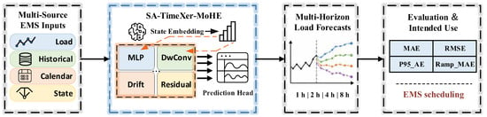
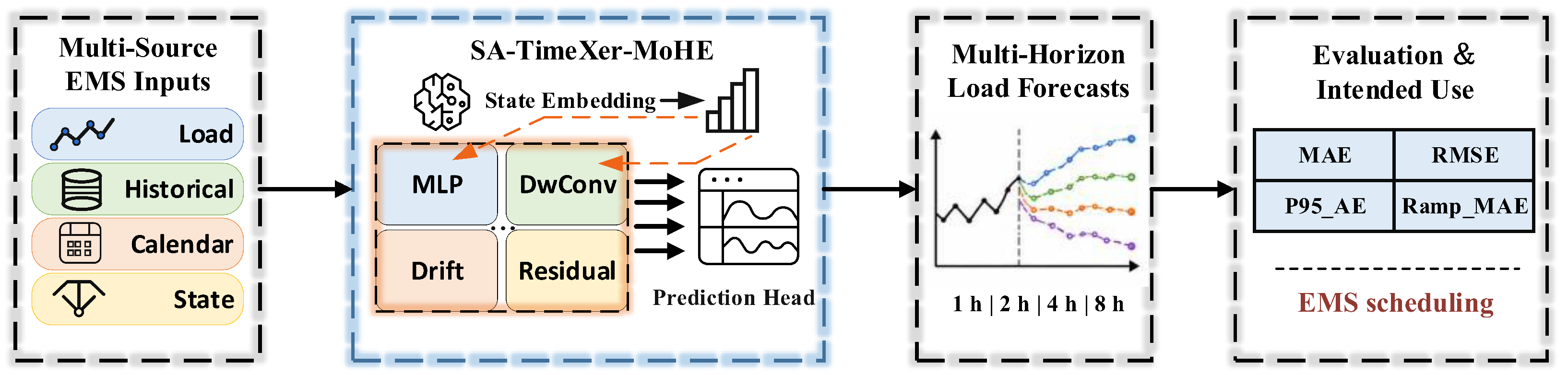
The overall research workflow is summarized in Figure 1. Multi-source EMS variables are organized according to their availability at the forecasting time, and SA-TimeXer-MoHE combines covariate-enhanced temporal modeling with scenario-aware heterogeneous experts to generate multi-horizon load forecasts. The forecasts are evaluated using average, tail, and ramp-tracking errors and are intended to provide predictive inputs for subsequent EMS scheduling.

Figure 1. Overview of the research workflow, from availability-aware organization of multi-source EMS inputs through SA-TimeXer-MoHE forecasting to multi-horizon outputs, condition-relevant evaluation, and intended downstream use.

The main contributions of this work can be summarized as follows:

• We formulate multi-horizon load forecasting for a grid-side storage EMS under an explicit information-availability constraint. The inputs are separated into the directly logged load target, historical-only physical measurements, deterministic future calendar variables, and operating-scenario covariates, so that unavailable future operating measurements are not used as model inputs.
• We introduce SA-MoHE, which replaces the homogeneous TimeXer feed-forward module with four structurally distinct experts: MLP, depthwise convolution, drift, and residual experts. Their motivation is operator-level diversity: position-wise nonlinear transformation, finite-neighborhood mixing, explicit first-order change sensitivity, and identity-preserving correction, respectively. These properties are architectural inductive biases rather than a predefined physical decomposition of the load. A sparse Top-K router conditions expert selection jointly on learned token representations and nine EMS scenario variables, allowing the selected transformation path to depend on the reported operating condition.
• We evaluate SA-TimeXer-MoHE on a 5 min real-world EMS dataset over four forecasting horizons using average, tail, and ramp-tracking errors. The evaluation includes sequential component ablations, expert-activation analysis, and dataset-adapted experiments on two public load datasets, while keeping downstream operational claims outside the demonstrated evidence.

The remainder of this paper is organized as follows. Section 2 formulates the EMS short-term load forecasting problem, defines the availability-aware covariate groups, and introduces the TimeXer forecasting backbone. Section 3 presents SA-TimeXer-MoHE, including the heterogeneous experts, scenario-aware router, and sparse output fusion. Section 4 reports the experimental setup and the comparative, ablation, public-dataset transfer, and expert-activation results. Section 5 presents the conclusions and summarizes the evidence boundaries and future work.

2. Problem Formulation and Covariate-Aware Forecasting Backbone

2.1. Problem Definition

In an EMS, short-term load forecasting is positioned between the data-perception and scheduling-optimization layers. Its primary role is to provide predictive information on future load variations for energy-storage operation, peak regulation, and rolling scheduling. Unlike conventional univariate load forecasting, EMS load series are influenced not only by historical electricity-consumption behavior and temporal periodicity but also by PV output, energy-storage operating states, grid-interconnection power, and scheduling actions. Therefore, this paper formulates short-term load forecasting as a sequence-forecasting problem enhanced by multi-source covariates rather than as an autoregressive problem based solely on historical load observations.

Assume that EMS data are collected at a fixed sampling interval $\mathrm{\Delta }t$; this study uses a 5 min resolution. Let $y_t$ denote the directly logged active-load channel recorded by the EMS at time step t. This channel is the only forecasting target in this study: the model does not forecast net load, PV generation, PCS or battery power, or grid-interconnection power. PV output, storage-operation measurements, grid-interconnection power, and temporal variables are used only as auxiliary covariates according to their forecast-time availability. To avoid information leakage and characterize EMS operating states, the inputs are divided into four categories: the endogenous sequence ${\mathbf{y}}_{t-L+1:t}$, historical covariates ${\mathbf{X}}_{t-L+1:t}^{his}$, known future covariates ${\mathbf{X}}_{t+1:t+H}^{fut}$, and scenario covariates ${\mathbf{s}}_t$. Given a historical observation window of length L, the model predicts only the future active-load sequence over a horizon of length H. The forecasting task is expressed as:

$${\widehat{\mathbf{y}}}_{t+1:t+H}=F_{\theta }\left({\mathbf{y}}_{t-L+1:t},{\mathbf{X}}_{t-L+1:t}^{his},{\mathbf{X}}_{t+1:t+H}^{fut},{\mathbf{s}}_t\right)$$

(1)

where $F_{\theta }$ denotes the forecasting model to be learned and ${\widehat{\mathbf{y}}}_{t+1:t+H}$ denotes the predicted load sequence over the next H time steps.

2.2. Multi-Source Covariate Modeling

This paper uses the directly logged active-load channel $y_t$ as the only forecasting target. In practical EMS terms, it is the directly acquired aggregate-load signal supplied to the forecasting module (the dataset field OT), and its predicted trajectory can be used as a demand input for storage dispatch, peak regulation, and rolling scheduling. It is neither reconstructed by algebraically combining photovoltaic (PV), power conversion system (PCS), battery, or grid-power channels, nor interpreted as grid import or export; those channels are treated exclusively as auxiliary measurements. Historical covariates $X_{t-L+1:t}^{his}$ refer to operating-state variables observed before the forecasting time but unavailable over the future horizon. This paper uses total PV power, PV branch power, battery state of charge (SOC), PCS active power, grid-interconnection power, and battery-branch power as historical covariates. The historical covariate vector at a single time step can be written as:

$${\mathbf{x}}_t^{his}=[P_t^{pv,total},P_t^{pv,1},\dots ,P_t^{pv,m},SO{C}_t,P_t^{pcs},P_t^{grid},P_t^{bat,1},\dots ,P_t^{bat,n}]$$

(2)

where $P_t^{pv,total}$ denotes the total PV power, $P_t^{pv,i}$ denotes the PV power of the i-th module branch, $SO{C}_t$ denotes the energy-storage SOC, $P_t^{pcs}$ denotes the PCS active power, $P_t^{grid}$ denotes the grid-interconnection power, and $P_t^{bat,j}$ denotes the battery power of the j-th branch. These variables characterize the operating state of the grid-side energy-storage EMS before the forecasting window, including renewable-generation fluctuations, storage charging and discharging behavior, point-of-interconnection power exchange, and the available regulation margin of the storage system. The future values of SOC, PCS power, grid-interconnection power, and battery-branch power usually depend on subsequent scheduling actions and system operation and are therefore unavailable at the forecasting time. Consequently, only their historical observations are used, thereby avoiding leakage of future information. Let $t_0$ denote the forecast issue time, defined as the timestamp of the latest completed 5 min EMS observation available to the forecaster. The encoder receives the load and measured operating variables only over $t_0-L+1:t_0$, and the prediction target is $y_{t_0+1:t_0+H}$. Thus, the directly logged values at $t_0$, including $y_{t_0}$, are historical observations rather than unknown forecast targets. If the most recent telemetry interval is incomplete or delayed in deployment, the issue time must be moved back to the latest completed interval.

Known future covariates ${\mathbf{x}}_{t+1:t+H}^{fut}$ comprise information available in advance over the forecasting horizon, mainly calendar variables and operating-period labels. This paper uses hour, minute, weekday, workday indicator, holiday indicator, and scheduling-period indicator as known future covariates. These features are normalized to fixed numerical ranges and fed into the temporal embedding layer to help characterize periodic load variations, consistent with multi-horizon forecasting studies that exploit known temporal and exogenous information [36,37]. Such variables do not depend on future true loads or scheduling outcomes and can therefore be constructed at the forecasting time. The known future covariate vector for a future time step is written as:

$${\mathbf{x}}_t^{fut}=[hou{r}_t,minut{e}_t,weekda{y}_t,workda{y}_t,holida{y}_t,to{u}_t]$$

(3)

where $hou{r}_t$, $minut{e}_t$, and $weekda{y}_t$ denote the hour, minute, and weekday information, respectively; $workda{y}_t$ indicates whether the day is a workday; $holida{y}_t$ indicates whether the day is a holiday; and $to{u}_t$ denotes the peak/flat/valley tariff-period label. By incorporating known future covariates, the model can perceive the temporal position and operating period of the forecasting horizon in advance, thereby strengthening its ability to model daily periodicity, weekly periodicity, and electricity-use period patterns.

In addition to historical and known future covariates, we construct a nine-dimensional EMS scenario-covariate vector, as shown in Table 1, to describe the observed operating condition and guide the subsequent scenario-aware sparse routing of heterogeneous experts. Scenario vectors are constructed only for historical indices $u\in [t_0-L+1,t_0]$; no realized measurement from $t_0+1:t_0+H$ is used. For compactness, the generic subscript t in the following feature definitions denotes an observed timestamp satisfying $t\le t_0$.

$${\mathbf{s}}_t=[s_t^{day},s_t^{workday},s_t^{peak},s_t^{pv\_active},s_t^{soc\_low},s_t^{ramp\_high},s_t^{pv\_pen},s_t^{soc\_margin},s_t^{grid\_stress}]$$

(4)

Table 1. Definition, interpretation, and inference-time source of the scenario covariates. Binary variables identify discrete operating states, whereas continuous variables describe state intensity. All measured inputs are restricted to completed observations at or before the forecast issue time $t_0$.

Scenario Feature	Description	Type	Inference-Time Source
Day	Whether the system is in a daytime period	Binary	Timestamp of historical observation $u\le t_0$
Workday	Whether the day is a workday	Binary	Timestamp of historical observation $u\le t_0$
Peak	Whether the system is in a peak-load period	Binary	Timestamp of historical observation $u\le t_0$
PV active	Whether PV generation is active	Binary	Observed $P_u^{pv,total}$, $u\le t_0$
Low SOC	Whether the energy-storage SOC is at a low level	Binary	Observed $SO{C}_u$, $u\le t_0$
Ramp	Whether the sample belongs to a high-ramp condition	Binary	Observed $y_u$ and $y_{u-1}$, $u\le t_0$
PV ratio	Relative PV contribution intensity	Continuous	Observed $P_u^{pv,total}$ and $y_u$, $u\le t_0$
SOC margin	Relative SOC position within the training distribution	Continuous	Observed $SO{C}_u$, $u\le t_0$
Grid stress	Grid-interconnection power magnitude and change intensity	Continuous	Observed $P_u^{grid}$ and $P_{u-1}^{grid}$, $u\le t_0$

All data-dependent thresholds are estimated exclusively from the training subset. Let $Q_p^{tr}(·)$ denote the p-th quantile calculated from training samples. The Day indicator equals one for $07:00\le hou{r}_t<19:00$, the Workday indicator equals one when $weekda{y}_t<5$, and the Peak indicator equals one for $hou{r}_t\in \{11,12,\dots ,18\}$. The PV-active indicator is set to one when $|P_t^{pv,total}|>Q_{0.10}^{tr}\left(\right|P^{pv,total}\left|\right)$, the Low-SOC indicator is set to one when $SO{C}_t\le Q_{0.30}^{tr}\left(SOC\right)$, and the high-ramp indicator is set to one when $|y_t-y_{t-1}|\ge Q_{0.75}^{tr}\left(\right|y_u-y_{u-1}\left|\right)$. At inference, the latest ramp value is therefore computed from $y_{t_0}$ and $y_{t_0-1}$, both of which belong to the completed encoder history. It is not computed from $y_{t_0+1}$ or any later realized load.

The continuous PV-ratio feature first measures the absolute PV-to-load ratio and then scales it by its training-set 95th percentile:

$$r_t^{pv}={\displaystyle \frac{|P_t^{pv,total}|}{|y_t|+ϵ}},s_t^{pv\_pen}=\mathrm{clip}\left({\displaystyle \frac{r_t^{pv}}{Q_{0.95}^{tr}\left(r^{pv}\right)}},0,1\right)$$

(5)

where $ϵ={10}^{-6}$ avoids division by zero and $\mathrm{clip}(x,0,1)=\min (1,\max (0,x\left)\right)$. This bounded feature describes the relative PV contribution intensity without allowing extreme low-load ratios to dominate routing.

The SOC-margin feature represents the current SOC position relative to the central range of the training distribution:

$$s_t^{soc\_margin}=\mathrm{clip}\left({\displaystyle \frac{SO{C}_t-Q_{0.30}^{tr}\left(SOC\right)}{Q_{0.70}^{tr}\left(SOC\right)-Q_{0.30}^{tr}\left(SOC\right)}},0,1\right)$$

(6)

A value of zero indicates an SOC at or below the training-set 30th percentile, whereas a value of one indicates an SOC at or above the 70th percentile. Thus, this feature is a quantile-normalized SOC-position indicator rather than a direct estimate of bidirectional regulation capacity.

The grid-stress score combines the magnitude and first-order change of the grid-interconnection power:

$$s_t^{grid\_stress}=\mathrm{clip}\left[{\displaystyle \frac{1}{2}}\left({\displaystyle \frac{|P_t^{grid}|}{Q_{0.95}^{tr}\left(|P^{grid}|\right)}}+{\displaystyle \frac{|\mathrm{\Delta }{P}_t^{grid}|}{Q_{0.95}^{tr}(|\mathrm{\Delta }{P}^{grid}|)}}\right),0,1\right]$$

(7)

where $\mathrm{\Delta }{P}_t^{grid}=P_t^{grid}-P_{t-1}^{grid}$. A larger score indicates a larger grid-power magnitude, a more rapid grid-power change, or both, relative to the training distribution.

Through the above variable partitioning, this paper forms a multi-source covariate input system for EMS-oriented load forecasting. Historical operating measurements are never substituted for unknown future values, while calendar variables are used only when they are deterministically available over the forecast horizon. This availability-aware organization is intended to prevent use of unavailable future information [30,37].

2.3. TimeXer-Based Forecasting Backbone

In grid-side EMS load forecasting, the target load series and multi-source covariates are strongly coupled. Directly concatenating all variables along the same temporal dimension can easily overlook differences between the target variable and covariates in physical meaning, availability, and temporal granularity. Therefore, this paper adopts TimeXer as the covariate-enhanced forecasting backbone to model the interaction between the endogenous load series and external covariates [30].

The core idea of TimeXer is to distinguish endogenous variables from exogenous variables. For the target load sequence to be forecast, the model uses patch-wise representations to capture local time variations and long-range dependencies of the load itself. For external covariates, the model uses variate-wise representations, embedding each covariate sequence as a variable-level token. This avoids the noise and computational overhead caused by overly fine-grained modeling of exogenous variables. In this paper, load is treated as the endogenous target variable, while historical and known future covariates are treated as external auxiliary information. EMS scenario covariates are not fed into the TimeXer backbone as ordinary exogenous variables; instead, they guide expert routing in the subsequent SA-MoHE module.

TimeXer first performs patch embedding on the endogenous load sequence and introduces a learnable global token. Meanwhile, each covariate sequence is embedded as a variable-level token. The embedding process can be simplified as:

$${\mathbf{P}}^{en},{\mathbf{g}}^{en}=\mathrm{EndoEmbed}\left({\mathbf{y}}_{t-L+1:t}\right),$$

(8)

$${\mathbf{V}}^{ex}=\mathrm{ExoEmbed}\left({\mathbf{X}}^{cov}\right)$$

(9)

where $P^{en}$ denotes the patch-level endogenous tokens obtained from the historical load sequence, $g^{en}$ denotes the learnable endogenous global token, and $V^{ex}$ denotes the exogenous variable tokens obtained from historical covariates and known future covariates. Endogenous patch tokens are mainly used to describe short-term fluctuations and temporal dependencies within the load sequence, while the global token serves as an information bridge between the endogenous load series and exogenous covariates.

In the TimeXer encoder, the model first captures temporal dependencies within the load series through endogenous self-attention and then introduces covariate information through exogenous-to-endogenous cross-attention. This sequence preserves a target-centered workflow while allowing available auxiliary information to refine the representation. This process can be summarized as:

$${\tilde{\mathbf{H}}}^{en}=\mathrm{SelfAttn}\left([{\mathbf{P}}^{en},{\mathbf{g}}^{en}]\right)$$

(10)

$${\overline{\mathbf{g}}}^{en}=\mathrm{CrossAttn}\left({\tilde{\mathbf{g}}}^{en},{\mathbf{V}}^{ex},{\mathbf{V}}^{ex}\right)$$

(11)

where $[{\mathbf{P}}^{en},{\mathbf{g}}^{en}]$ denotes the concatenation of endogenous patch tokens and the global token, ${\tilde{\mathbf{H}}}^{en}$ denotes the target-load representation after endogenous self-attention, ${\tilde{\mathbf{g}}}^{en}$ is its updated global token, ${\overline{\mathbf{g}}}^{en}$ is the global token after cross-attention, and $\mathrm{CrossAttn}(·)$ denotes the cross-attention operation. Through this structure, the model can adaptively extract useful information from PV generation, energy storage, grid-interconnection power, and time features according to the current load state and inject it into the global representation of the target load.

Both the endogenous self-attention and cross-attention operators are implemented using dense FullAttention without causal masking. Each operator uses eight attention heads, an attention factor of 1, and an attention-dropout rate of 0.1. Attention matrices are not returned during the reported experiments. Thus, the implementation does not use ProbSparse or de-stationary attention variants.

After multiple encoding layers, the final endogenous representation is fed into the prediction head to output the load forecasts for the future H time steps:

$${\widehat{\mathbf{y}}}_{t+1:t+H}=\mathrm{Projection}\left({\mathbf{H}}^{en}\right)$$

(12)

where ${\mathbf{H}}^{en}$ denotes the endogenous load representation after TimeXer encoding, and $\mathrm{Projection}(·)$ denotes the prediction mapping function.

3. SA-TimeXer-MoHE Model

In Section 2, EMS short-term load forecasting was formulated as a sequence-forecasting problem enhanced by multi-source covariates, and TimeXer was adopted as the backbone for modeling interactions between the target load sequence and external covariates. However, EMS load variations are affected by PV output, energy-storage states, grid-interconnection power, and temporal periodicity, and their patterns differ across operating conditions. The feed-forward network in the original TimeXer encoder adopts a homogeneous structure and applies the same nonlinear transformation path to all samples and tokens, preventing explicit specialization for heterogeneous load patterns.

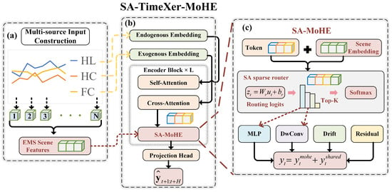
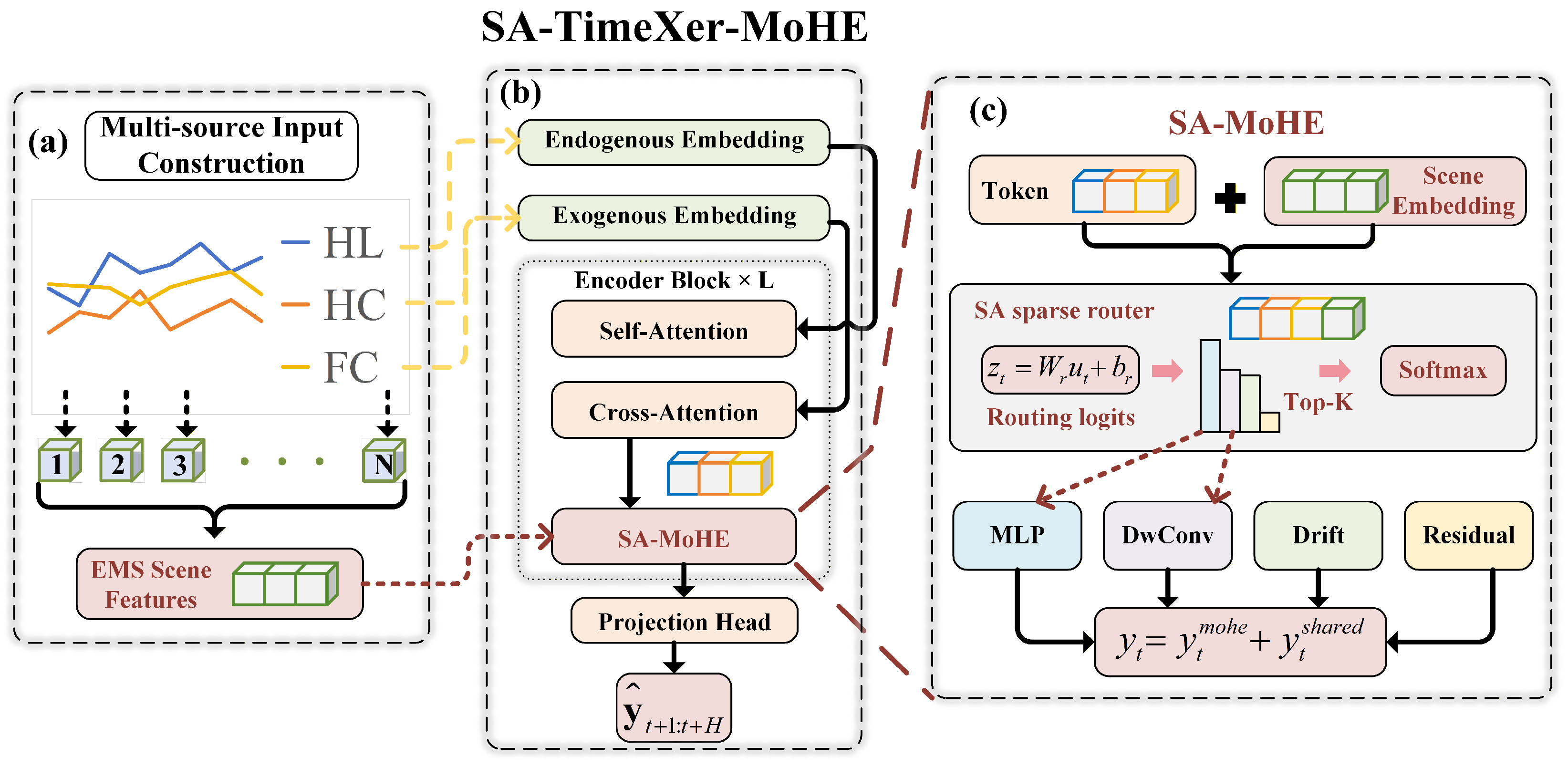
To address this issue, this paper proposes the SA-TimeXer-MoHE forecasting model, as shown in Figure 2. Based on the TimeXer covariate-enhanced backbone, the model introduces a MoHE module consisting of MLP, DwConv, Drift, and Residual experts. EMS scenario covariates are incorporated into expert selection through sparse routing. The different expert structures provide alternative inductive biases for stable nonlinear mappings, local temporal dependence, differenced representations, and residual mappings. The routing analysis reported later is descriptive; the present experiments do not by themselves establish a causal physical role for any individual expert.

Figure 2. Overall architecture of the proposed SA-TimeXer-MoHE model. The model consists of three components: (a) A multi-source input construction module, which partitions inputs into historical load sequence (HL), historical covariates (HC), known future covariates (FC), and EMS scenario covariates according to information availability at the forecasting time. (b) The SA-TimeXer-MoHE forecasting framework, which uses TimeXer as the covariate-enhanced backbone and models interactions between the target load sequence and multi-source covariates through endogenous embedding, exogenous embedding, self-attention, and cross-attention, while replacing the original feed-forward network with the SA-MoHE module. (c) The SA-MoHE module, which jointly uses token representations and scenario embeddings to generate routing scores. After Softmax normalization, Top-K sparse selection, and renormalization over the selected experts, the module activates the corresponding MLP, DwConv, Drift, or Residual expert and fuses its output with the shared branch to obtain updated token representations.

Before presenting the detailed equations, the model workflow can be understood in four stages. First, the target load and auxiliary variables are partitioned according to forecast-time availability. Second, TimeXer encodes the historical load and permitted covariates into interacting target and exogenous representations. Third, the scenario-aware router uses the encoded token and historical EMS scenario variables to select a sparse subset of the four heterogeneous experts. Finally, the selected expert outputs are fused with the shared branch and projected to the multi-horizon load forecast. Figure 2 maps these stages to the corresponding model components; the equations below specify the operations within each stage.

3.1. MoHE Module

This subsection details the heterogeneous-expert transformation stage in the preceding workflow: the four experts receive compatible encoded representations but apply different mathematical operators before sparse selection and fusion. In standard Transformer-like architectures, the feed-forward network is usually implemented as a position-wise FFN, which applies the same parameters and transformation path to all inputs. Its expressive capability is therefore constrained by a homogeneous operator family. To introduce complementary transformation mechanisms while retaining compatible hidden dimensions, this paper replaces the homogeneous FFN in the TimeXer encoder with a MoHE module consisting of MLP, DwConv, Drift, and Residual experts. The motivation for this expert set is based on their mathematical operators rather than an assumed one-to-one decomposition of the measured load into physical components. The four experts provide, respectively, position-wise nonlinear channel mixing, finite-neighborhood token mixing, an explicit first-order change term, and an identity-preserving correction path. Their outputs have the same dimension and can therefore be selected and fused by a common sparse router.

Given the input to layer l, ${\mathbf{X}}^{\left(l\right)}\in {\mathbb{R}}^{B\times T\times d}$, where B is the batch size, T is the number of ordered encoder-token positions, and d is the hidden dimension, expert i is denoted by $E_i(·)$, $i=1,2,3,4$. The MLP expert uses the standard position-wise FFN architecture and preserves the generic nonlinear channel-mixing capability of the original Transformer. Its computation is given by:

$$E_{MLP}\left(X\right)=W_2\sigma (W_{1}X+b_1)+b_2$$

(13)

where $W_1\in {\mathbb{R}}^{d\times d_{ff}}$, $W_2\in {\mathbb{R}}^{d_{ff}\times d}$, and $\sigma (·)$ denotes the nonlinear activation function. Because the same transformation is applied independently at every ordered position, its cross-position Jacobian satisfies $\partial E_{MLP}{\left(\mathbf{X}\right)}_t/\partial {\mathbf{X}}_j=0$ for $j\ne t$. Thus, the MLP expert supplies a position-wise nonlinear reference operator without explicitly encoding neighborhood mixing or first-order changes. It may represent baseline nonlinear relations, but it is not predefined as a periodic-load component.

The DwConv expert introduces depthwise separable one-dimensional convolution into the FFN. For the ordered input representation $\mathbf{X}$, depthwise convolution is first performed along the token-position dimension, followed by pointwise convolution for channel expansion and compression:

$$H_{dw}=DWCon{v}_k\left(X\right)$$

(14)

$$E_{DwConv}\left(X\right)=PWCon{v}_2\left(\sigma \left(PWCon{v}_1\left(H_{dw}\right)\right)\right)$$

(15)

where k is the convolution kernel size, $DWCon{v}_k(·)$ performs position-neighborhood convolution independently on each hidden channel, and $PWCon{v}_1$ and $PWCon{v}_2$ correspond to feature expansion and reduction, respectively. For an odd kernel size k, the output at position t can depend only on the finite neighborhood ${\mathcal{N}}_k\left(t\right)=\{j:|j-t|\le (k-1)/2\}$. This locality property distinguishes DwConv from the position-wise MLP and provides an architectural bias toward local interactions. It does not, by itself, identify those interactions as a particular physical disturbance such as PV fluctuation.

The Drift expert augments a basic MLP branch with an explicit first-order difference projection, with the final output given by:

$$E_{Drift}\left(X\right)=H_{base}+H_{drift}=W_2\sigma \left(W_{1}X\right)+W_d\mathrm{\Delta }X$$

(16)

$$\mathrm{\Delta }{X}_t=X_t-X_{t-1}$$

(17)

For the first ordered position, $\mathrm{\Delta }{X}_1=0$, or equivalently $X_0=X_1$. The differencing operator has two relevant properties: it eliminates a position-invariant component, $\mathrm{\Delta }{\mathbf{X}}_t=0$ when ${\mathbf{X}}_t=\mathbf{c}$, and returns the local slope for an affine representation, $\mathrm{\Delta }{\mathbf{X}}_t=\mathbf{b}$ when ${\mathbf{X}}_t=\mathbf{a}+t\mathbf{b}$. Consequently, the additional projection provides explicit sensitivity to representation changes that is absent from a purely position-wise MLP. This is an operator-level change bias and does not establish that the expert uniquely represents a physical state-drift component.

The Residual expert introduces an identity-preserving path inside the FFN so that the nonlinear branch learns a correction to the current representation. Its structure is given by:

$$E_{Res}\left(X\right)=X+W_2\sigma \left(W_{1}X\right)$$

(18)

When the input and output dimensions are inconsistent, the residual path is aligned through a linear mapping:

$$E_{Res}\left(X\right)=W_{s}X+W_2\sigma \left(W_{1}X\right)$$

(19)

where $W_s$ is the residual projection matrix. When the dimensions agree, the deviation from the input is exactly the learned nonlinear correction, $E_{Res}\left(\mathbf{X}\right)-\mathbf{X}=W_2\sigma \left(W_1\mathbf{X}\right)$, and the input–output Jacobian contains an identity term. The expert can therefore preserve an existing representation while learning a bounded correction when the nonlinear branch is small. This identity-preserving property motivates its inclusion as an alternative transformation path; it does not imply that it is exclusively responsible for ramps, noise, or large forecasting residuals.

Taken together, the four operators differ in cross-position dependence, explicit change sensitivity, and identity preservation. These are verifiable structural distinctions, but they do not constitute a theorem that the load can be decomposed into four corresponding physical components. The router learns how to use the available operators from the forecasting objective. Accordingly, the component ablation evaluates the benefit of replacing a homogeneous MLP expert set with the heterogeneous set as a whole, whereas the subsequent activation heatmap is interpreted only as descriptive routing evidence rather than proof of a unique physical function for an individual expert.

3.2. Scenario-Aware Routing Mechanism

This subsection describes the selection step in the workflow: it explains how historical scenario information and the current token representation are combined to determine which expert paths are activated. Conventional Mixture of Experts (MoE) or MoHE models usually route only according to input token representations, meaning that expert selection is entirely data-driven [31,32,34]. For grid-side EMS load forecasting, different operating scenarios have explicit engineering meanings. To enable experts to adaptively specialize according to load operating states, we introduce a scenario-aware mechanism into the conventional MoE router.

First, the nine-dimensional EMS scenario vectors over the encoder history $t_0-L+1:t_0$ are aligned with the endogenous patch tokens. For each non-overlapping encoder patch, the scenario vectors within that historical patch are averaged; the global-token scenario vector is the mean of the patch-level vectors. Only this historical, token-aligned scenario tensor is supplied to the router. Scenario vectors associated with the label or forecast interval are not passed to the model. Denoting a token-aligned scenario vector by ${\mathbf{s}}_t$, it is projected into a d-dimensional embedding through a linear mapping:

$$h_t^s=\varphi \left({\mathbf{s}}_t\right)=W_s{\mathbf{s}}_t+b_s$$

(20)

where $W_s\in {\mathbb{R}}^{d\times 9}$ and $b_s\in {\mathbb{R}}^d$. Then, the time-series hidden state and scenario embedding are concatenated to obtain $u_t$, and the expert logits are generated through the routing mapping:

$${\mathbf{z}}_t^{scene}=W_r{\mathbf{u}}_t+b_r=W_r[{\mathbf{x}}_t;{\mathbf{h}}_t^s]+b_r$$

(21)

where $z_t^{scene}$ denotes the unnormalized selection scores of N experts produced by the scenario-conditioned router, and $W_r$ and $b_r$ are its weight matrix and bias term, respectively. For completeness, the implementation also contains a token-only router, $z_t^{base}=W_b{x}_t+b_b$, and an optional non-learned scenario-prior branch. The general routing formulation implemented by the model is

$${\tilde{\mathbf{z}}}_t=(1-\alpha ){\mathbf{z}}_t^{base}+\alpha {\mathbf{z}}_t^{scene}+\beta {\mathbf{p}}_t,$$

(22)

where $\alpha \in [0,1]$ is a fixed mixing coefficient between the token-only and scenario-conditioned router logits, $\beta \ge 0$ is a fixed strength coefficient for the optional prior, and neither coefficient is optimized by backpropagation. The endpoint $\alpha =0$ recovers token-only routing, whereas $\alpha =1$ uses only the learned scenario-conditioned router. The optional prior follows the routed-expert order $[\mathrm{MLP},\mathrm{DwConv},\mathrm{Drift},\mathrm{Residual}]$ and is explicitly defined as

$${\mathbf{p}}_t=\left[\begin{array}{c}{s}_t^{workday}(1-s_t^{ramp\_high})\\ s_t^{peak}+s_t^{pv\_active}+s_t^{ramp\_high}\\ s_t^{day}{s}_t^{pv\_active}\\ s_t^{soc\_low}+s_t^{ramp\_high}\end{array}\right].$$

(23)

This vector is an optional engineering heuristic rather than a learned parameter or a physical decomposition. Its first entry favors the MLP slot during workday, non-high-ramp states; the second combines peak-period, active-PV, and high-ramp indicators for the DwConv slot; the third combines daytime and active-PV indicators for the Drift slot; and the fourth combines low-SOC and high-ramp indicators for the Residual slot. The three continuous scenario covariates remain inputs to the learned scenario-conditioned router but are not used in this optional rule-based vector.

Importantly, the prior branch was disabled in all experiments reported in this paper. The evaluated configuration fixes $\alpha =1$, $\beta =0$, and $\tau =1$, so that ${\tilde{\mathbf{z}}}_t={\mathbf{z}}_t^{scene}$. Consequently, the reported expert selections are learned end-to-end from the token representation, nine scenario covariates, and forecasting objective; they are not produced by the rule-based assignments in ${\mathbf{p}}_t$. Under $\beta =0$, changing the numerical contents of ${\mathbf{p}}_t$ has exactly zero effect on the routing logits or forecasts. The settings $\alpha =1$ and $\beta =0$ are therefore implementation-defining endpoint choices rather than hyperparameters selected from a performance-based sensitivity search. The expert routing weights ${\pi }_t$ at time step t are calculated by Softmax:

$${\mathit{\pi }}_t=\mathrm{Softmax}\left({\displaystyle \frac{{\tilde{\mathbf{z}}}_t}{\tau }}\right)=[{\pi }_{t,1},{\pi }_{t,2},\dots ,{\pi }_{t,N}]$$

(24)

where $\tau >0$ is a fixed temperature coefficient. A larger $\tau$ makes the probability distribution smoother, whereas a smaller $\tau$ makes it sharper. With the reported $K=1$ routing, division by a positive temperature does not change the identity of the maximum-logit expert at inference, although it changes the pre-selection probabilities used during training. Here, N denotes the number of experts, and ${\pi }_{t,i}$ denotes the importance weight of the i-th expert at the current time step.

Through this routing mechanism, expert weights can depend on both token representations and the reported EMS scenario features. This makes the routing inputs explicit, but expert-activation plots should be interpreted as descriptive evidence rather than proof that a specific expert has a unique physical function in a particular scenario.

3.3. Sparse Expert Selection and Output Fusion

After the scenario-aware routing mechanism obtains the response weights of different experts, invoking all experts at every time step would fully utilize the expressive capacity of the expert set but would also incur considerable computational overhead and potentially weaken specialization among experts. Therefore, SA-TimeXer-MoHE introduces a sparse expert selection mechanism. The reported configuration contains four routed experts and uses $K=1$, so each token activates only the expert with the highest routing probability. The shared DwConv branch remains active for every token and is not included in the Top-K selection.

According to the computed weights, the model selects the Top-K experts and obtains the activated expert set ${\mathcal{K}}_t$. Experts that are not selected do not contribute to output fusion at the current time step. The selected expert outputs are then fused in a weighted manner:

$$y_t^{mohe}=\sum _{i\in {\mathcal{K}}_t}{\overline{\pi }}_{t,i}{E}_i\left(x_t\right)$$

(25)

where $E_i(·)$ denotes the i-th expert network, ${\overline{\pi }}_{t,i}$ denotes its routing weight renormalized over the selected set, and $x_t$ is the hidden representation at the current time step. With $K=1$, the renormalized weight of the selected routed expert equals one, and different tokens can therefore select different experts according to their routing probabilities. To reduce excessive dependence on a single routed expert under sparse routing, the model also retains a shared mapping branch:

$${\tilde{y}}_t^{shared}=g_t·y_t^{shared}$$

(26)

where $y_t^{shared}=E_{shared}\left(x_t\right)$ is the output of the shared DwConv FFN and $g_t=\mathrm{Sigmoid}\left(W_g{x}_t\right)$ is a learned gating coefficient that adaptively controls its contribution. The shared branch does not participate in Top-K selection, but provides a stable basic mapping for all time steps and supplements general information that the selected routed expert may miss. This design allows the model to select condition-dependent heterogeneous transformations while maintaining overall forecasting stability through the shared branch. Finally, the MoHE layer output is jointly formed by the sparse expert branch and the shared branch:

$$y_t=y_t^{mohe}+{\tilde{y}}_t^{shared}$$

(27)

The sparse expert-selection and output-fusion mechanism gives SA-TimeXer-MoHE dynamic expert invocation capability. The Top-K mechanism limits the participation of low-weight experts, while scenario-aware routing associates expert weights with the reported load operating states. The resulting forecasts can serve as predictive inputs for subsequent peak-regulation and energy-storage scheduling tasks; downstream operational benefits are not evaluated in this study.

4. Results and Experimental Analysis

4.1. Experimental Settings

This section reports experiments on one real-world EMS dataset and two public load datasets. The public-dataset experiments examine whether the framework remains applicable after its scenario inputs are reconstructed from fields available in each dataset; they do not represent a direct transfer of the original EMS-specific scenario definition.

Real-world EMS dataset. The proprietary dataset was derived from anonymized operational records of a grid-side energy-storage station in Indonesia. The study interval extends from 00:00 on 1 January to 23:55 on 28 February 2026 (UTC+08:00), corresponding to a calendar coverage of 59 days. The raw EMS telemetry was acquired at approximately 30 s intervals and contains both station-level and branch-level electrical measurements. The forecasting target is the directly logged active-load channel rather than a load series reconstructed from other power channels.

The raw records were processed by parsing and sorting timestamps, converting measurement channels to numerical form, retaining the latest record for duplicate timestamps, aligning the telemetry to a regular time axis, and filling missing points by time-based interpolation. The synchronized measurements were then averaged over non-overlapping 5 min intervals. The resulting modeling table contains 16,992 chronologically ordered and unique timestamps, equivalent to 288 observations per day, and contains no missing values in the channels selected for model input. For every training, validation, and test window, only the scenario tensor aligned with the encoder history is forwarded to SA-TimeXer-MoHE; scenario values aligned with the label and forecast interval are not consumed by the model. Table 2 provides a compact forecast-time availability map of the measured and derived variables used in the experiments.

Table 2. Forecast-time availability and modeling roles of the real-world EMS variables. “Historical only” denotes completed observations at or before the issue time $t_0$; future physical measurements are excluded from model inputs. Equipment identifiers and rated operating parameters are omitted because of data-provider confidentiality restrictions.

Category	Variables	Unit	Availability and Modeling Role
Forecast target	Directly logged active load	kW	Historical values are encoder inputs; future values are prediction targets only and are never model inputs
PV operation	Total PV output and five PV-branch outputs	kW	Historical only; future PV measurements are excluded; used as covariates and for historical scenario construction
Storage operation	SOC, PCS active power, total battery power, and five battery-branch powers	%, kW	Historical only; all future storage-operation measurements are excluded
Grid interaction	Grid-interconnection active power	kW	Historical only; future grid-power measurements are excluded; used for historical grid-stress construction
Temporal context	Hour, minute, weekday, workday, holiday, and scheduling-period labels	–	Timestamp-derived and known for both the historical window and forecast horizon

All power measurements retain the sign conventions of the source EMS and are expressed in kilowatts (kW). Calendar and scheduling-period variables were generated only from timestamps and therefore do not contain future measurements. To avoid temporal leakage, the 5 min sequence was kept in chronological order and divided into training, validation, and test subsets using a 7:1:2 ratio; the later observations were not randomly mixed into the training subset. To ensure a fair comparison across models, a StandardScaler was fitted using only the training subset and was subsequently applied to the training, validation, and test subsets. Any reversible sample-wise normalization performed internally by a forecasting model was inverted at its output. For physical interpretability, error metrics on the real-world EMS dataset are mapped from the standardized target scale back to kW using the training-target standard deviation ${\sigma }_y=42.37484$ kW. The reported error metrics are presented in kW first, with corresponding standardized values in parentheses for reproducibility. Station names, geographic coordinates, equipment identifiers, rated capacities, and other commercially sensitive information were excluded before analysis.

Public datasets. We adopted the widely used ElectricityLoadDiagrams2011–2014 (ECL) dataset and the Load Forecasting Track of the Global Energy Forecasting Competition 2014 (GEFCom2014), hereafter referred to as GEFCom-L [38,39]. GEFCom-L contains electricity-load series and associated temporal information and is used to examine the model under a public load-forecasting setting. Both public datasets contain periodic, trending, and locally fluctuating load patterns. Because they do not provide the EMS-specific physical variables used in the real-world dataset, only dataset-specific generic temporal-state features can be constructed for the router.

All deep learning models are implemented under a unified experimental environment. The final hyperparameter settings are listed in Table 3.

Table 3. Architecture and training configuration used in the reported experiments.

Architecture Setting	Value	Training Setting	Value
Input sequence length (steps)	288	Batch size	32
Forecast horizon (steps)	12/24/48/96	Training epochs	50
Encoder layers	3	Early stopping	5
Label length (steps)	24	Initial learning rate	0.00005
Patch length	24	Train/Val/Test ratio	7:1:2
Model dimension $d_{\mathrm{model}}$	512	Learning-rate schedule	type1
FFN dimension $d_{\mathrm{ff}}$	512	Automatic mixed precision	Disabled
Attention heads	8	Optimizer	Adam
Scenario-vector dimension	9	Random seeds	2021–2025
Routed experts	MLP, DwConv, Drift, Residual	Validation method	Chronological holdout
DwConv kernel size	3	Dataset scaling	Training-set StandardScaler
Sparse routing	$K=1$	Dropout	0.1
Shared branch	Always-active DwConv	Activation	GELU
Routing coefficients $(\alpha ,\beta ,\tau )$	$(1,0,1)$	Time embedding	timeF

Separate experiments are conducted for forecast horizons of 12, 24, 48, and 96 steps while keeping the remaining settings fixed. For every model and forecast horizon, five independent training runs are performed using the fixed random seeds 2021, 2022, 2023, 2024, and 2025. The same seed set is applied consistently to all compared models. The numerical results reported in the tables are the arithmetic means across the five runs. Complete run-level values are unavailable for reliable post hoc reconstruction of standard deviations; therefore, no variability statistic or formal significance test is reported, and the comparisons are interpreted descriptively. In each run, the Python (v3.11.14), NumPy (v1.23.5), and PyTorch (v2.11.0+cu126) random generators are initialized with the designated seed. Under the type1 learning-rate schedule, the learning rate is halved after each epoch. The model uses a dropout rate of 0.1, GELU activation, time-feature embedding (timeF), six data-loading workers, and no automatic mixed-precision training. For SA-TimeXer-MoHE, the four routed experts are MLP, DwConv, Drift, and Residual, the sparse-routing parameter is set to $K=1$, and an always-active shared DwConv branch is retained in each MoHE layer. The reported configuration uses the fixed routing coefficients $\alpha =1$, $\beta =0$, and $\tau =1$; the optional rule-based scenario-prior branch is therefore inactive, and these three coefficients are not learned.

Training objective. The model is trained using an MSE prediction loss together with a routing load-balancing term and two lightweight condition-oriented terms:

$${\mathcal{L}}^{\left(e\right)}={\mathcal{L}}_{pred}+{\lambda }_{aux}^{\left(e\right)}{\mathcal{L}}_{lb}+{\lambda }_{peak}{\mathcal{L}}_{peak}+{\lambda }_{ramp}{\mathcal{L}}_{ramp},$$

(28)

where e denotes the training epoch and ${\mathcal{L}}_{pred}$ is the MSE between the forecast and target sequences. The load-balancing loss ${\mathcal{L}}_{lb}$ is calculated from the pre-selection router probabilities: for each MoHE layer, the mean routing probability assigned to each expert is computed over the tokens in the current batch, and the sum of their squared mean probabilities is multiplied by the number of experts; the resulting values are then averaged across MoHE layers. The high-load loss ${\mathcal{L}}_{peak}$ is the MSE over target points at or above the 0.9 quantile of the observed target values in the current training batch. The ramp loss ${\mathcal{L}}_{ramp}$ is the MSE between the first-order differences of adjacent forecast steps and those of the corresponding target steps.

The maximum auxiliary-loss weight is $5\times {10}^{-4}$. It is zero in epoch 1, increases linearly over epochs 2–4, and remains at $5\times {10}^{-4}$ thereafter. Both ${\lambda }_{peak}$ and ${\lambda }_{ramp}$ are set to $1\times {10}^{-3}$. The global gradient norm is clipped at 1.0 during training. Model selection and early stopping are based on the validation MSE rather than the auxiliary training terms.

4.2. Evaluation Metrics

In addition to low average error, EMS forecasting benefits from accurate characterization of peak loads and rapid ramping processes because deviations during these periods can reduce the quality of predictive inputs available for operational decisions. MAE and RMSE are used as conventional forecast-accuracy measures [40]. In addition, we define the 95th-percentile absolute error and ramping error as condition-relevant metrics for the evaluated EMS forecasting task.

$$\mathrm{MAE}={\displaystyle \frac{1}{N}}{\displaystyle \sum _{i=1}^N}|{\widehat{y}}_i-y_i|$$

(29)

$$\mathrm{RMSE}=\sqrt{{\displaystyle \frac{1}{N}}\sum _{i=1}^N{({\widehat{y}}_i-y_i)}^2}$$

(30)

$$P95\_AE=P_{95}\left(|{\widehat{y}}_i-y_i|\right)$$

(31)

$$\mathrm{Ramp}\_\mathrm{MAE}={\displaystyle \frac{1}{M(H-1)}}{\displaystyle \sum _{m=1}^M}{\displaystyle \sum _{h=2}^H}\left|({\widehat{y}}_{m,h}-{\widehat{y}}_{m,h-1})-(y_{m,h}-y_{m,h-1})\right|$$

(32)

where N is the total number of forecast–target pairs used to calculate MAE, RMSE, and P95_AE; M is the number of test forecasting windows; and H is the forecast horizon. The quantities $y_{m,h}$ and ${\widehat{y}}_{m,h}$ denote the observed and predicted values, respectively, at step h of forecasting window m. Thus, Ramp_MAE calculates adjacent-step changes within each forecasting window and does not form differences across window boundaries. MAE and RMSE evaluate the overall error level, P95_AE characterizes the upper tail of the absolute-error distribution, and Ramp_MAE measures ramp-tracking error. Because standardization is linear, all four error metrics are converted by $E_{\mathrm{kW}}={\sigma }_y{E}_{\mathrm{std}}$, where ${\sigma }_y=42.37484$ kW is estimated only from the training target. Together, these metrics assess average accuracy, tail-error behavior, and dynamic-change tracking under the evaluated EMS conditions.

4.3. Main Experiments

To evaluate SA-TimeXer-MoHE for EMS short-term load forecasting, Transformer, DLinear, PatchTST, iTransformer, and the original TimeXer are selected as comparison models [30,41,42,43,44]. Experiments use forecast horizons of 12, 24, 48, and 96 steps, corresponding to 1, 2, 4, and 8 h at a 5 min sampling interval. The results are listed in Table 4.

Table 4. Forecasting results of different models on the real-world EMS dataset at forecast horizons $H\in \{12,24,48,96\}$. Each error cell reports kW first, with the corresponding standardized value in parentheses. Values are arithmetic means across five independent runs using random seeds 2021–2025; variability statistics are not reported because complete run-level values are unavailable for reliable post hoc reconstruction. “Avg” is retained only as a compact overall summary and should not replace horizon-specific comparison. Lower values indicate better forecasting performance, and the best results are highlighted in bold.

Model	Pre_Steps	MAE	RMSE	P95_AE	Ramp_MAE
SA-TimeXer-MoHE	12	12.42 (0.293)	17.37 (0.410)	37.71 (0.890)	7.25 (0.171)
	24	14.07 (0.332)	18.86 (0.445)	39.07 (0.922)	7.29 (0.172)
	48	14.96 (0.353)	19.32 (0.456)	39.58 (0.934)	7.33 (0.173)
	96	15.42 (0.364)	20.13 (0.475)	41.78 (0.986)	7.20 (0.170)
	Avg	14.24 (0.336)	18.94 (0.447)	39.54 (0.933)	7.29 (0.172)
TimeXer	12	13.69 (0.323)	18.48 (0.436)	39.15 (0.924)	7.84 (0.185)
	24	15.76 (0.372)	20.09 (0.474)	39.96 (0.943)	8.14 (0.192)
	48	15.72 (0.371)	20.47 (0.483)	42.37 (1.000)	7.50 (0.177)
	96	16.40 (0.387)	21.31 (0.503)	43.31 (1.022)	7.54 (0.178)
	Avg	15.38 (0.363)	20.09 (0.474)	41.19 (0.972)	7.75 (0.183)
PatchTST	12	13.81 (0.326)	18.60 (0.439)	39.79 (0.939)	7.46 (0.176)
	24	15.76 (0.372)	20.72 (0.489)	39.79 (0.939)	7.46 (0.176)
	48	15.76 (0.372)	20.72 (0.489)	43.01 (1.015)	7.63 (0.180)
	96	17.63 (0.416)	22.42 (0.529)	44.66 (1.054)	7.50 (0.177)
	Avg	15.76 (0.372)	20.64 (0.487)	41.82 (0.987)	7.50 (0.177)
iTransformer	12	14.28 (0.337)	19.11 (0.451)	39.92 (0.942)	8.09 (0.191)
	24	14.96 (0.353)	19.92 (0.470)	41.99 (0.991)	8.01 (0.189)
	48	15.64 (0.369)	20.76 (0.490)	43.56 (1.028)	8.05 (0.190)
	96	16.44 (0.388)	21.40 (0.505)	43.77 (1.033)	8.09 (0.191)
	Avg	15.34 (0.362)	20.30 (0.479)	42.33 (0.999)	8.05 (0.190)
DLinear	12	13.48 (0.318)	18.52 (0.437)	39.37 (0.929)	7.42 (0.175)
	24	14.66 (0.346)	19.70 (0.465)	41.15 (0.971)	7.42 (0.175)
	48	15.59 (0.368)	20.64 (0.487)	43.05 (1.016)	7.37 (0.174)
	96	16.27 (0.384)	21.15 (0.499)	43.31 (1.022)	7.37 (0.174)
	Avg	15.00 (0.354)	20.00 (0.472)	41.74 (0.985)	7.42 (0.175)
Transformer	12	13.52 (0.319)	17.84 (0.421)	37.76 (0.891)	7.67 (0.181)
	24	16.99 (0.401)	21.48 (0.507)	42.25 (0.997)	7.59 (0.179)
	48	16.36 (0.386)	21.19 (0.500)	43.86 (1.035)	7.46 (0.176)
	96	19.24 (0.454)	25.04 (0.591)	48.35 (1.141)	7.42 (0.175)
	Avg	16.53 (0.390)	21.40 (0.505)	43.05 (1.016)	7.54 (0.178)

Under the reported experimental configuration, SA-TimeXer-MoHE obtains the lowest mean values in Table 4 across the evaluated horizons and metrics. Its mean MAE, RMSE, P95_AE, and Ramp_MAE are 14.24, 18.94, 39.54, and 7.29 kW, respectively, (standardized values: 0.336, 0.447, 0.933, and 0.172), corresponding to mean values 7.4%, 5.7%, 4.0%, and 6.0% lower than those of the original TimeXer. These aggregated results show favorable mean performance for the combined covariate-aware heterogeneous-expert configuration; they do not isolate the independent contribution of scenario routing.

The horizon-specific rows provide information that is not captured by the Avg row alone. For SA-TimeXer-MoHE, MAE increases from 12.42 kW at 1 h to 15.42 kW at 8 h, RMSE increases from 17.37 to 20.13 kW, and P95_AE increases from 37.71 to 41.78 kW, reflecting the greater uncertainty of longer-horizon forecasting. In contrast, its Ramp_MAE remains within 7.20–7.33 kW across all four horizons, indicating comparatively stable ramp tracking. Operationally, the 1 h forecast is most relevant to near-term corrective control, the 2–4 h forecasts support rolling scheduling, and the 8 h forecast provides a longer look-ahead for operating-plan adjustment. Therefore, model selection for a specific EMS function should use the corresponding horizon-specific rows rather than the Avg row alone.

The baseline models also exhibit clear differences. TimeXer and PatchTST perform well at some forecast horizons, but their errors increase noticeably as the forecast horizon becomes longer. For example, when the forecast horizon is 96 steps, PatchTST reaches an MAE of 17.63 kW and an RMSE of 22.42 kW, indicating insufficient sustained modeling capability for load variation at long forecast horizons. iTransformer and DLinear show relatively stable overall performance, but they remain inferior to SA-TimeXer-MoHE in high-percentile error and ramping error. Transformer has average MAE and RMSE values of 16.53 and 21.40 kW, respectively, which are among the highest errors of all models. This suggests that the conventional Transformer structure has relatively limited adaptability to local fluctuations and long-range dependencies in this load forecasting task.

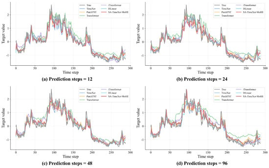
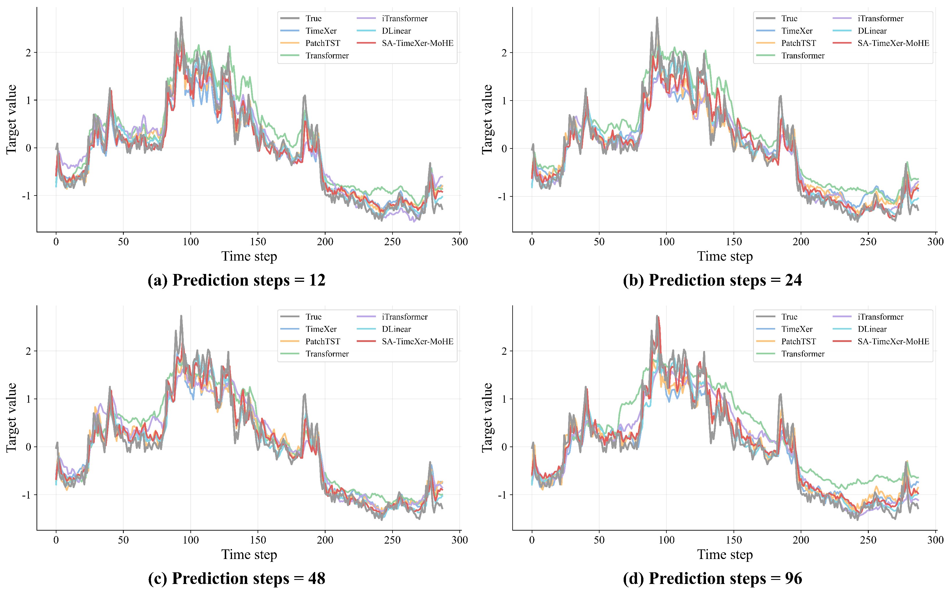
Figure 3 retains all comparison curves to provide a qualitative view of different prediction behaviors; each model is identified by a distinct color in the legend, and the complete quantitative comparison is given in Table 4. DLinear is selected as the main baseline reference in the accompanying discussion because it has the lowest Avg MAE, Avg RMSE, and Avg Ramp_MAE among the baselines (three of four aggregate metrics); TimeXer has a slightly lower Avg P95_AE.

Figure 3. Prediction results of all compared models on the real-world EMS dataset. To preserve the completeness of the qualitative comparison, all baseline forecasts are displayed and identified by distinct legend colors. Complete quantitative comparisons are provided in Table 4. Subfigures (a–d) correspond to forecast horizons of 12, 24, 48, and 96 steps, respectively.

As shown in Figure 3, SA-TimeXer-MoHE follows the observed load trend closely across the four displayed horizons, including rapid increases, peak fluctuations, and decline stages. Retaining all baselines allows qualitative comparison of oversmoothing, local lag, and deviations around high-variation regions, while Table 4 should be used for the quantitative ranking.

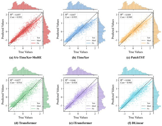
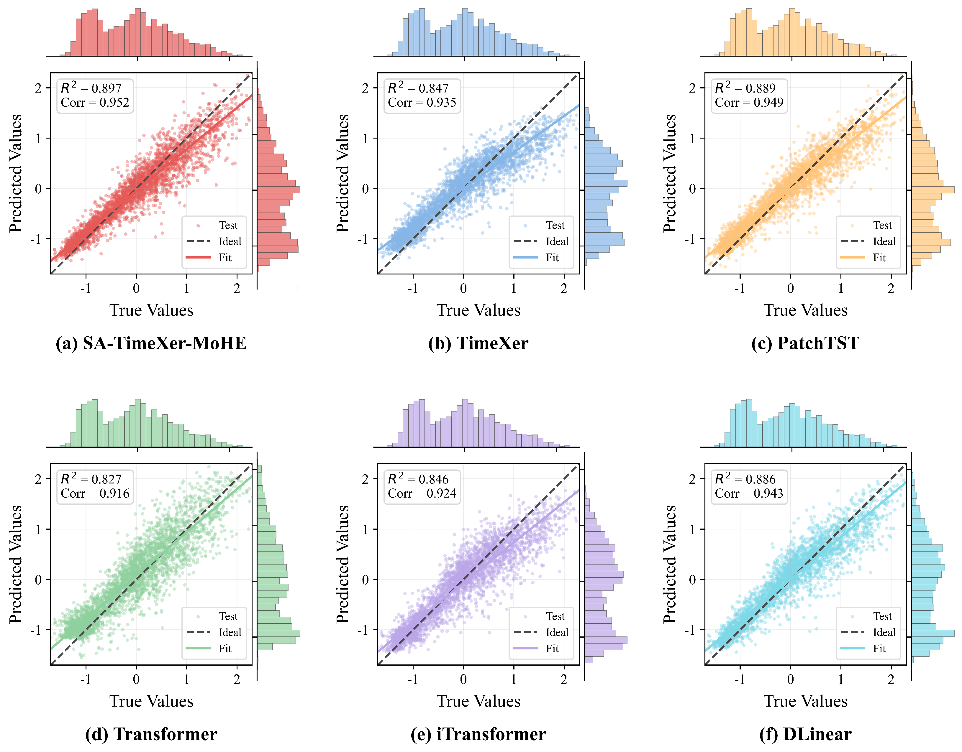
As shown in Figure 4, the prediction scatter of SA-TimeXer-MoHE forms a compact linear distribution, with most points concentrated near the ideal line. This indicates that the model effectively characterizes true load variation. It achieves an $R^2$ of 0.897 and a $Corr$ of 0.952, demonstrating both strong numerical fitting capability and good preservation of the load variation trend. In comparison, although the baseline models also show relatively high overall correlation, their scatter points are more dispersed, especially in some high-load intervals, indicating room for improvement in capturing load amplitude variation.

Figure 4. Scatter distributions of predicted versus true values for each model on the real-world EMS dataset with a forecast horizon of 12 steps. The horizontal and vertical axes represent the standardized true and predicted load values, respectively, and the dashed line is the ideal prediction line. Points closer to this line indicate better agreement between predicted and true values. The coefficient of determination $R^2$ and correlation coefficient $Corr$ characterize goodness of fit and trend consistency, respectively.

Overall, SA-TimeXer-MoHE achieves the lowest mean values for all four metrics among the models compared on the real-world EMS dataset. The aggregated results show favorable mean forecasting accuracy, tail-error control, and ramp tracking under the evaluated settings, while maintaining close agreement with the observed load trend.

4.4. Component Ablation Results

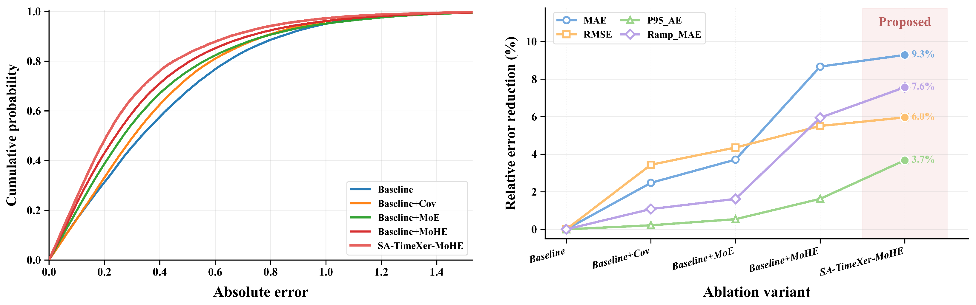
Table 5 reports a sequential component ablation at a forecast horizon of $H=12$ steps (1 h). The variants add multi-source covariates, an MoE module, heterogeneous experts, and scenario-aware routing in turn. The table reports arithmetic means across five independent runs. Because run-level variability statistics and a formal paired significance result are unavailable, the cumulative comparison is interpreted descriptively rather than as a statistical attribution of each individual component.

Table 5. Ablation results of different model variants at a forecast horizon of $H=12$ steps (1 h). Each error cell reports kW first, with the corresponding standardized value in parentheses. Values are arithmetic means across five independent runs using random seeds 2021–2025; variability statistics are not reported because complete run-level values are unavailable for reliable post hoc reconstruction. TimeXer is used as the baseline model; Baseline + Cov denotes the original TimeXer enhanced with multi-source covariates; Baseline + MoE further introduces four homogeneous MLP experts; Baseline + MoHE replaces the homogeneous expert set with MLP, DwConv, Drift, and Residual experts while retaining the expert-mixture framework; and SA-TimeXer-MoHE further adds the scenario-aware routing mechanism.

Model	MAE	RMSE	P95_AE	Ramp_MAE
Baseline	13.69 (0.323)	18.48 (0.436)	39.15 (0.924)	7.84 (0.185)
Baseline + Cov	13.35 (0.315)	17.84 (0.421)	39.07 (0.922)	7.75 (0.183)
Baseline + MoE	13.18 (0.311)	17.67 (0.417)	38.94 (0.919)	7.71 (0.182)
Baseline + MoHE	12.50 (0.295)	17.46 (0.412)	38.52 (0.909)	7.37 (0.174)
SA-TimeXer-MoHE	12.42 (0.293)	17.37 (0.410)	37.71 (0.890)	7.25 (0.171)

Bold values indicate the best results.

Compared with the original TimeXer, the variant with multi-source covariates has lower mean values for all four reported metrics. Subsequent cumulative variants also show lower mean values across the five runs. These changes are compatible with the intended roles of covariate information, expert capacity, and heterogeneous transformations, but the mean differences alone do not establish statistical significance.

Within this sequential comparison, the transition from Baseline + MoE to Baseline + MoHE retains the covariate-enhanced backbone and expert-mixture framework but changes the expert composition from four homogeneous MLP transformations to the heterogeneous operator set. The corresponding mean MAE, RMSE, P95_AE, and Ramp_MAE values are approximately 5.1%, 1.2%, 1.1%, and 4.4% lower, respectively, based on Table 5. This repeated-run comparison supports the complementarity of the heterogeneous set as a whole under the evaluated settings; it does not identify a unique physical role for any single expert. Adding scenario-aware routing produces the lowest mean values in this sequential comparison, but its marginal change from Baseline + MoHE is small. Run-level variability statistics, routing-specific controls, and formal paired testing are still required before claiming an independent scenario-routing effect.

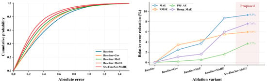
The left CDF panel shows that the curve generally shifts toward the upper-left as successive modules are added. Thus, under the same absolute-error threshold, the enhanced variants contain a higher proportion of low-error samples. The SA-TimeXer-MoHE curve is uppermost over the displayed range, indicating the most concentrated error distribution among the evaluated variants. The relative-error-reduction panel further summarizes the gains from successive modifications. The larger reductions in MAE and Ramp_MAE indicate improvements in overall accuracy and ramp tracking, respectively.

Taken together, Table 5 and Figure 5 show a monotonic pattern of lower mean values as the listed components are cumulatively added. The evidence supports the full configuration across the five repeated runs under the evaluated settings, while the independent effect of each component remains to be verified through dedicated controls and formal paired testing.

Figure 5. Ablation experimental results at a forecast horizon of $H=12$ steps (1 h) from the perspectives of error distribution and module contribution. The left panel shows the cumulative distribution function (CDF) curve of absolute errors on the standardized target-variable scale for different models, and the right panel shows the relative error reduction of each ablation variant. The CDF curve describes the cumulative probability of prediction error under different thresholds. The closer a curve is to the upper-left quadrant, the higher the proportion of low-error samples and the lower the proportion of high-error samples under the same error threshold, indicating more stable prediction results.

4.5. Public-Dataset Transfer Experiments

To examine behavior under different load distributions, we evaluate a dataset-adapted version of SA-TimeXer-MoHE on ECL and GEFCom-L; the results are shown in Table 6. These experiments do not use the original EMS-specific physical scenario covariates. For both datasets, the router input retains four non-zero features constructed from the completed encoder history: Day ($07:00\le hou{r}_t<19:00$), Workday ($weekda{y}_t<5$), Peak ($hou{r}_t\in \{11,\dots ,18\}$), and high ramp ($|y_t-y_{t-1}|\ge Q_{0.75}^{tr}\left(\right|\mathrm{\Delta }y\left|\right)$). The five unavailable EMS-specific components—PV active, Low SOC, PV ratio, SOC margin, and Grid stress—are set to zero. Thus, ECL uses timestamp indicators and the historical change of the target consumer series; GEFCom-L uses the same router features, while its weather variables remain ordinary exogenous inputs to the forecasting backbone rather than EMS scenario variables. All quantile-based quantities are fitted on the corresponding training subset only.

Table 6. Forecasting results of different models on the ECL and GEFCom-L datasets. Each entry is the arithmetic mean across five independent runs using random seeds 2021–2025; variability statistics are not reported because complete run-level values are unavailable for reliable post hoc reconstruction.

Datasets	Models	MAE	RMSE	P95_AE	Ramp_MAE
ECL	SA-TimeXer-MoHE	0.415	0.581	1.161	0.180
	TimeXer	0.440	0.595	1.239	0.187
	PatchTST	0.441	0.620	1.278	0.181
	iTransformer	0.427	0.559	1.170	0.189
	DLinear	0.534	0.710	1.479	0.195
	Transformer	0.483	0.642	1.350	0.200
GEFCom-L	SA-TimeXer-MoHE	0.282	0.398	0.803	0.082
	TimeXer	0.294	0.407	0.855	0.086
	PatchTST	0.313	0.423	0.870	0.087
	iTransformer	0.300	0.423	0.901	0.090
	DLinear	0.309	0.425	0.884	0.089
	Transformer	0.310	0.412	0.836	0.133

On ECL, SA-TimeXer-MoHE obtains the lowest mean MAE, P95_AE, and Ramp_MAE among the compared models, whereas iTransformer obtains the lowest mean RMSE. Relative to TimeXer and based on the rounded values in Table 6, its mean MAE, RMSE, P95_AE, and Ramp_MAE values are approximately 5.7%, 2.4%, 6.3%, and 3.7% lower, respectively. On GEFCom-L, it obtains the lowest mean values for all four metrics, which are approximately 4.1%, 2.2%, 6.1%, and 4.7% lower than those of TimeXer. These results show lower mean errors for the dataset-adapted configurations under the reported settings, but the gains are generally smaller than on the EMS dataset. A plausible explanation is that only four generic timing-and-ramp proxies remain informative for public-dataset routing, whereas the EMS router additionally observes PV, SOC, and grid-stress variables that distinguish operating regimes more directly. Differences in sampling resolution, load composition, exogenous inputs, and baseline difficulty may also affect relative gains; therefore, the cross-dataset percentages are interpreted descriptively rather than as a causal attribution to any single factor.

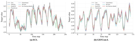
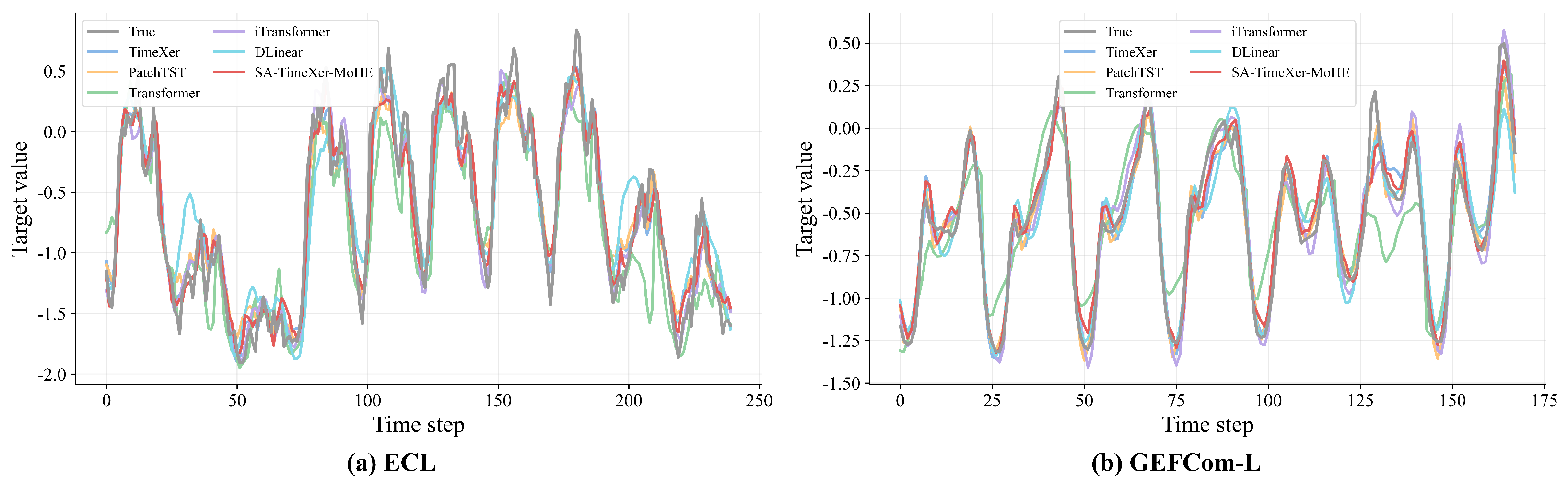
Figure 6 likewise retains all baseline forecasts to show qualitative differences across the public datasets, with each model identified by a distinct color in the legend. Table 6 provides the complete quantitative comparison: iTransformer is the strongest ECL baseline on MAE, RMSE, and P95_AE, whereas TimeXer is the strongest GEFCom-L baseline on MAE, RMSE, and Ramp_MAE.

Figure 6. Prediction results of all compared models on the public datasets (ECL and GEFCom-L). All baselines are retained and identified by distinct legend colors to allow direct visual comparison of different error patterns. The corresponding quantitative comparisons are reported in Table 6.

Figure 6 provides qualitative comparisons on the public datasets by retaining all baseline forecasts. This presentation illustrates differences in peak/valley tracking and local fluctuation modeling, while Table 6 provides the corresponding quantitative evaluation. On ECL, SA-TimeXer-MoHE achieves the lowest MAE, P95_AE, and Ramp_MAE, whereas iTransformer attains a lower RMSE. On GEFCom-L, SA-TimeXer-MoHE achieves the best performance across all four reported metrics.

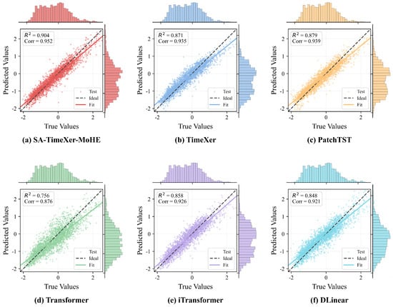
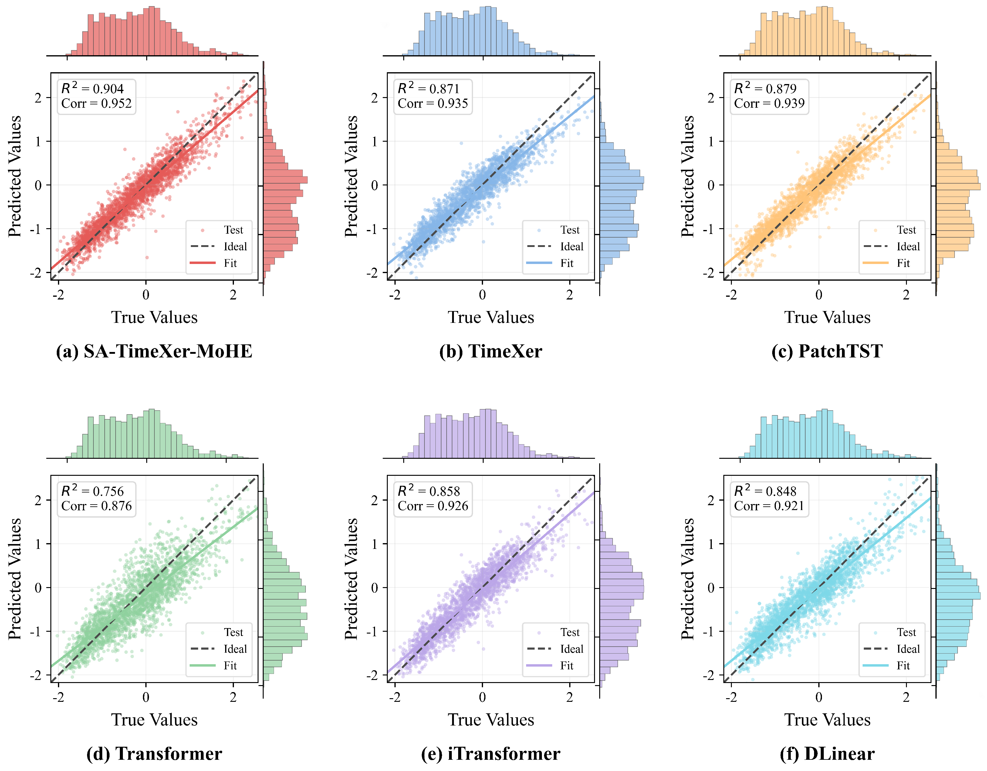
Figure 7 shows that the SA-TimeXer-MoHE scatter distribution is concentrated near the ideal line. Its reported $R^2$ and $Corr$ values are 0.904 and 0.952, respectively, indicating close numerical agreement and trend consistency on ECL.

Figure 7. Scatter distributions of predicted versus true values for each model on the ECL dataset.

Taken together, the two public-dataset evaluations show that the heterogeneous-expert framework can be configured with generic temporal-state features. They do not establish direct transferability of the EMS-specific routing mechanism across sites, seasons, or operating regimes.

4.6. Analysis of the SA-MoHE

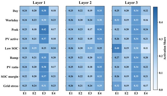
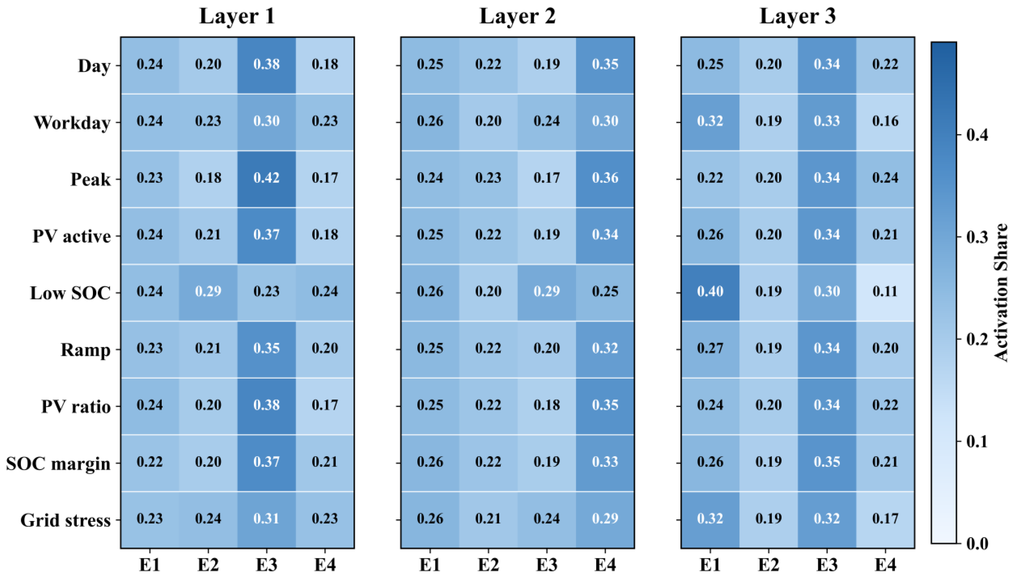
To further analyze the role of the SA-MoHE mechanism in SA-TimeXer-MoHE, we calculate the average activation proportions of each expert under different EMS operating scenarios and visualize them using an expert-activation heatmap, as shown in Figure 8.

Figure 8. Expert activation heatmap under different EMS operating scenarios. A darker color indicates a higher activation proportion.

In Layer 1, Expert E3 has the highest or near-highest activation proportion in most displayed scenarios. In the Low SOC row, E2 reaches 0.29. These values describe the router behavior in the evaluated model run, but they do not establish that a scenario uniquely requires the corresponding expert or that the expert has a verified physical function.

In Layer 2, E4 is relatively prominent in several rows, while E3 reaches 0.29 in the Low SOC row and E4 reaches 0.29 in the Grid stress row. The differences show that routing is not identical across all reported conditions, but a controlled comparison with shuffled scenario labels and repeated seeds is needed to assess whether these patterns are robust and attributable to the scenario inputs.

In Layer 3, E1 and E3 have relatively higher activation proportions, whereas E4 is less active than in Layer 2. This layer-dependent pattern is descriptive and should not be interpreted as proof of a fixed hierarchy of expert functions.

Overall, the activation distributions vary across layers and reported conditions. They provide an interpretable summary of routing behavior for this run, while rigorous evidence for scenario-specific specialization requires additional controlled analyses beyond the present study. The present evaluation is limited to one real-world energy-storage station and two public load datasets. These limitations define the scope of the reported evidence and separate demonstrated forecasting behavior from broader deployment claims. Moreover, the public datasets use reconstructed generic temporal-state features rather than the original EMS-specific operating variables. Future work will extend the evaluation to additional stations, seasons, and larger repeated-run studies, and will assess the effects of forecasting accuracy on downstream storage scheduling and operational performance.

5. Conclusions

This work develops the SA-TimeXer-MoHE framework for multi-horizon load forecasting in grid-side energy-storage EMSs. SA-TimeXer-MoHE replaces the TimeXer feed-forward module with heterogeneous experts and provides EMS scenario features to sparse expert routing. Across the four evaluated horizons on the real-world EMS dataset, SA-TimeXer-MoHE obtains the lowest reported mean values for all four metrics among the compared models. Relative to the original TimeXer, its mean MAE, RMSE, P95_AE, and Ramp_MAE values are 7.4%, 5.7%, 4.0%, and 6.0% lower, respectively. Ablation experiments showed favorable mean changes from the evaluated heterogeneous-expert components. The public dataset results further show that the framework can be adapted to load datasets with different available variables. These aggregated results highlight the potential of SA-TimeXer-MoHE to provide more accurate predictive inputs for rolling charge–discharge scheduling, peak regulation, grid-power exchange planning, and coordination among loads, PV generation, and energy storage. The framework therefore provides a promising forecasting basis for predictive EMS operation. Future work will evaluate its generalization across additional stations and seasons, quantify model reliability through larger repeated-seed and probabilistic studies, and examine the independent contribution of scenario-aware routing through dedicated controls. The forecasts will also be integrated with PV, price, and rolling-scheduling models in a closed-loop EMS to assess their effects on operating cost, peak shaving, SOC-constraint satisfaction, and battery cycling.

References

- Zia, M.F.; Elbouchikhi, E.; Benbouzid, M. Microgrids energy management systems: A critical review on methods, solutions, and prospects. Appl. Energy 2018, 222, 1033–1055. [Google Scholar] [CrossRef] [Scilit]
- Zahraoui, Y.; Alhamrouni, I.; Mekhilef, S.; Basir Khan, M.R.; Seyedmahmoudian, M.; Stojcevski, A.; Horan, B. Energy Management System in Microgrids: A Comprehensive Review. Sustainability 2021, 13, 10492. [Google Scholar] [CrossRef] [Scilit]
- Garcia Vera, Y.E.; Dufo-Lopez, R.; Bernal-Agustin, J.L. Energy Management in Microgrids with Renewable Energy Sources: A Literature Review. Appl. Sci. 2019, 9, 3854. [Google Scholar] [CrossRef] [Scilit]
- Caicedo-Vivas, J.S.; Alfonso-Morales, W. Short-Term Load Forecasting Using an LSTM Neural Network for a Grid Operator. Energies 2023, 16, 7878. [Google Scholar] [CrossRef] [Scilit]
- Akhtar, S.; Shahzad, S.; Zaheer, A.; Ullah, H.S.; Kilic, H.; Gono, R.; Jasinski, M.; Leonowicz, Z. Short-Term Load Forecasting Models: A Review of Challenges, Progress, and the Road Ahead. Energies 2023, 16, 4060. [Google Scholar] [CrossRef] [Scilit]
- Alfares, H.K.; Nazeeruddin, M. Electric load forecasting: Literature survey and classification of methods. Int. J. Syst. Sci. 2002, 33, 23–34. [Google Scholar] [CrossRef] [Scilit]
- Hippert, H.S.; Pedreira, C.E.; Souza, R.C. Neural networks for short-term load forecasting: A review and evaluation. IEEE Trans. Power Syst. 2001, 16, 44–55. [Google Scholar] [CrossRef] [Scilit]
- Taylor, J.W. Short-term electricity demand forecasting using double seasonal exponential smoothing. J. Oper. Res. Soc. 2003, 54, 799–805. [Google Scholar] [CrossRef] [Scilit]
- Hong, T.; Fan, S. Probabilistic electric load forecasting: A tutorial review. Int. J. Forecast. 2016, 32, 914–938. [Google Scholar] [CrossRef] [Scilit]
- Wang, Y.; Chen, Q.; Hong, T.; Kang, C. Review of Smart Meter Data Analytics: Applications, Methodologies, and Challenges. IEEE Trans. Smart Grid 2019, 10, 3125–3148. [Google Scholar] [CrossRef] [Scilit]
- Eren, Y.; Kucukdemiral, I. A comprehensive review on deep learning approaches for short-term load forecasting. Renew. Sustain. Energy Rev. 2024, 189, 114031. [Google Scholar] [CrossRef] [Scilit]
- Kerkau, S.; Sepasi, S.; Howlader, H.O.R.; Roose, L. Day-Ahead Net Load Forecasting for Renewable Integrated Buildings Using XGBoost. Energies 2025, 18, 1518. [Google Scholar] [CrossRef] [Scilit]
- Uddin, N.; Sepasi, S.; Ghorbani, R. Adaptive Residual-Transformer Ensemble for Day-Ahead Net-Load Forecasting in PV-Integrated Microgrids. IEEE Access 2026, 14, 118320–118336. [Google Scholar] [CrossRef] [Scilit]
- Hochreiter, S.; Schmidhuber, J. Long Short-Term Memory. Neural Comput. 1997, 9, 1735–1780. [Google Scholar] [CrossRef] [Scilit]
- Kong, W.; Dong, Z.Y.; Jia, Y.; Hill, D.J.; Xu, Y.; Zhang, Y. Short-Term Residential Load Forecasting Based on LSTM Recurrent Neural Network. IEEE Trans. Smart Grid 2019, 10, 841–851. [Google Scholar] [CrossRef] [Scilit]
- Muzaffar, S.; Afshari, A. Short-Term Load Forecasts Using LSTM Networks. Energy Procedia 2019, 158, 2922–2927. [Google Scholar] [CrossRef] [Scilit]
- Shi, H.; Xu, M.; Li, R. Deep learning for household load forecasting–A novel pooling deep RNN. IEEE Trans. Smart Grid 2018, 9, 5271–5280. [Google Scholar] [CrossRef] [Scilit]
- Chen, K.; Chen, K.; Wang, Q.; He, Z.; Hu, J.; He, J. Short-Term Load Forecasting with Deep Residual Networks. IEEE Trans. Smart Grid 2019, 10, 3943–3952. [Google Scholar] [CrossRef] [Scilit]
- Jahani, A.; Zare, K.; Mohammad Khanli, L. Short-term load forecasting for microgrid energy management system using hybrid SPM-LSTM. Sustain. Cities Soc. 2023, 98, 104775. [Google Scholar] [CrossRef] [Scilit]
- Zhou, H.; Zhang, S.; Peng, J.; Zhang, S.; Li, J.; Xiong, H.; Zhang, W. Informer: Beyond Efficient Transformer for Long Sequence Time-Series Forecasting. Proc. AAAI Conf. Artif. Intell. 2021, 35, 11106–11115. [Google Scholar] [CrossRef] [Scilit]
- Wu, H.; Xu, J.; Wang, J.; Long, M. Autoformer: Decomposition Transformers with Auto-Correlation for Long-Term Series Forecasting. In Proceedings of the 35th Conference on Neural Information Processing Systems, Virtual, 6–14 December 2021; Volume 34, pp. 22419–22430. [Google Scholar]
- Zhou, T.; Ma, Z.; Wen, Q.; Wang, X.; Sun, L.; Jin, R. FEDformer: Frequency Enhanced Decomposed Transformer for Long-term Series Forecasting. In Proceedings of the International Conference on Machine Learning, Baltimore, MD, USA, 17–23 July 2022; pp. 27268–27286. [Google Scholar]
- Liu, Y.; Wu, H.; Wang, J.; Long, M. Non-stationary Transformers: Exploring the Stationarity in Time Series Forecasting. In Proceedings of the 36th Conference on Neural Information Processing Systems, New Orleans, LA, USA, 28 November–9 December 2022; Volume 35, pp. 9881–9893. [Google Scholar]
- Wu, H.; Hu, T.; Liu, Y.; Zhou, H.; Wang, J.; Long, M. TimesNet: Temporal 2D-Variation Modeling for General Time Series Analysis. In Proceedings of the International Conference on Learning Representations, Kigali, Rwanda, 1–5 May 2023. [Google Scholar]
- Wang, S.; Wu, H.; Shi, X.; Hu, T.; Luo, H.; Ma, L.; Zhang, J.Y.; Zhou, J. TimeMixer: Decomposable Multiscale Mixing for Time Series Forecasting. In Proceedings of the International Conference on Learning Representations, Vienna, Austria, 7–11 May 2024. [Google Scholar]
- Kim, T.; Kim, J.; Tae, Y.; Park, C.; Choi, J.H.; Choo, J. Reversible Instance Normalization for Accurate Time-Series Forecasting against Distribution Shift. In Proceedings of the International Conference on Learning Representations, Virtual, 25–29 April 2022. [Google Scholar]
- Fan, W.; Wang, P.; Wang, D.; Wang, D.; Zhou, Y.; Fu, Y. Dish-TS: A General Paradigm for Alleviating Distribution Shift in Time Series Forecasting. Proc. AAAI Conf. Artif. Intell. 2023, 37, 7522–7529. [Google Scholar] [CrossRef] [Scilit]
- Li, S.; Cai, H. Short-Term Power Load Forecasting Using a VMD-Crossformer Model. Energies 2024, 17, 2773. [Google Scholar] [CrossRef] [Scilit]
- Sheng, W.; Yang, X.; Jia, D.; Liu, K.; Wang, Z.; Lin, R. Enhanced Transformer for Multivariate Load Forecasting: Timestamp Embedding and Convolution-Augmented Attention. Energies 2026, 19, 596. [Google Scholar] [CrossRef] [Scilit]
- Wang, Y.; Wu, H.; Dong, J.; Qin, G.; Zhang, H.; Liu, Y.; Qiu, Y.; Wang, J.; Long, M. TimeXer: Empowering Transformers for Time Series Forecasting with Exogenous Variables. In Proceedings of the 38th Conference on Neural Information Processing Systems, Vancouver, BC, Canada, 10–15 December 2024; Volume 37, pp. 2077–2100. [Google Scholar] [CrossRef] [Scilit]
- Jacobs, R.A.; Jordan, M.I.; Nowlan, S.J.; Hinton, G.E. Adaptive Mixtures of Local Experts. Neural Comput. 1991, 3, 79–87. [Google Scholar] [CrossRef] [Scilit]
- Shazeer, N.; Mirhoseini, A.; Maziarz, K.; Davis, A.; Le, Q.; Hinton, G.; Dean, J. Outrageously Large Neural Networks: The Sparsely-Gated Mixture-of-Experts Layer. In Proceedings of the International Conference on Learning Representations, Toulon, France, 24–27 April 2017. [Google Scholar]
- Lepikhin, D.; Lee, H.; Xu, Y.; Chen, D.; Firat, O.; Huang, Y.; Krikun, M.; Shazeer, N.; Chen, Z. GShard: Scaling Giant Models with Conditional Computation and Automatic Sharding. In Proceedings of the International Conference on Learning Representations, Virtual, 3–7 May 2021. [Google Scholar]
- Fedus, W.; Zoph, B.; Shazeer, N. Switch Transformers: Scaling to Trillion Parameter Models with Simple and Efficient Sparsity. J. Mach. Learn. Res. 2022, 23, 1–39. [Google Scholar]
- Wu, B. A Mixture-of-Experts Projection for Universal Gains in Transformer-Based Day-Ahead Net-Load Forecasting. SSRN 2025. [Google Scholar] [CrossRef] [Scilit]
- Salinas, D.; Flunkert, V.; Gasthaus, J.; Januschowski, T. DeepAR: Probabilistic forecasting with autoregressive recurrent networks. Int. J. Forecast. 2020, 36, 1181–1191, Erratum in Int. J. Forecast. 2021, 37, 1302–1303. https://doi.org/10.1016/j.ijforecast.2021.01.010. [Google Scholar] [CrossRef] [Scilit]
- Lim, B.; Arik, S.O.; Loeff, N.; Pfister, T. Temporal Fusion Transformers for interpretable multi-horizon time series forecasting. Int. J. Forecast. 2021, 37, 1748–1764. [Google Scholar] [CrossRef] [Scilit]
- Trindade, A. ElectricityLoadDiagrams20112014. UCI Machine Learning Repository, 12 March 2015. [CrossRef]
- Hong, T.; Pinson, P.; Fan, S.; Zareipour, H.; Troccoli, A.; Hyndman, R.J. Probabilistic energy forecasting: Global Energy Forecasting Competition 2014 and beyond. Int. J. Forecast. 2016, 32, 896–913. [Google Scholar] [CrossRef] [Scilit]
- Hyndman, R.J.; Koehler, A.B. Another look at measures of forecast accuracy. Int. J. Forecast. 2006, 22, 679–688. [Google Scholar] [CrossRef] [Scilit]
- Vaswani, A.; Shazeer, N.; Parmar, N.; Uszkoreit, J.; Jones, L.; Gomez, A.N.; Kaiser, L.; Polosukhin, I. Attention Is All You Need. In Proceedings of the 31st Conference on Neural Information Processing Systems, Long Beach, CA, USA, 4–9 December 2017; Volume 30. [Google Scholar]
- Zeng, A.; Chen, M.; Zhang, L.; Xu, Q. Are Transformers Effective for Time Series Forecasting? Proc. AAAI Conf. Artif. Intell. 2023, 37, 11121–11128. [Google Scholar] [CrossRef] [Scilit]
- Nie, Y.; Nguyen, N.H.; Sinthong, P.; Kalagnanam, J. A Time Series is Worth 64 Words: Long-term Forecasting with Transformers. In Proceedings of the International Conference on Learning Representations, Kigali, Rwanda, 1–5 May 2023. [Google Scholar]
- Liu, Y.; Hu, T.; Zhang, H.; Wu, H.; Wang, S.; Ma, L.; Long, M. iTransformer: Inverted Transformers Are Effective for Time Series Forecasting. In Proceedings of the International Conference on Learning Representations, Vienna, Austria, 7–11 May 2024. [Google Scholar]
Disclaimer/Publisher’s Note: The statements, opinions and data contained in all publications are solely those of the individual author(s) and contributor(s) and not of MDPI and/or the editor(s). MDPI and/or the editor(s) disclaim responsibility for any injury to people or property resulting from any ideas, methods, instructions or products referred to in the content. |
© 2026 by the authors. Licensee MDPI, Basel, Switzerland. This article is an open access article distributed under the terms and conditions of the Creative Commons Attribution (CC BY) license.