


Abstract
Coordinated scheduling of distributed generation (DG), battery energy storage systems (BESS) and demand response (DR) is needed to reduce grid procurement costs without compromising customer comfort or network constraints. This paper proposes a two-stage framework for a grid-connected IEEE 33-bus microgrid. In the first stage, the Red Panda Optimization (RPO) algorithm jointly determines the locations and ratings of renewable DG units and BESS by minimizing power losses and voltage deviation. In the second stage, five customer agents with different cost–comfort preferences and three BESS agents learn their hourly schedules under real-time pricing using multi-agent Q-learning. Two incentive regimes are compared within the same decentralized framework: a price-only, customer-driven regime and an incentive-coordinated regime in which the grid operator broadcasts a shadow-price signal. Compared with the DG-only case, the two regimes reduced daily demand by 2.36% and 12.21%, energy loss by 4.53% and 27.79%, and procurement cost by 3.25% and 12.99%, respectively. Customer load curtailment provides all the demand and loss reduction and most of the cost reduction, while BESS arbitrage lowers the cost by a further 0.62 and 0.61% points at the expense of slightly higher losses. The incentive design, rather than the control architecture, largely determines how these benefits are shared between the operator and customers.
1. Introduction
1.1. Motivation
Nowadays, energy management is a challenging task due to the integration of renewable energy resources and customers’ participation in buying and selling power from the grid. Along with this another issue is the weather dependency of renewable energy based DG’s which create the uncertainty in power production like solar based DG is only produce power during day time and wind based DG produce power only when the wind is available which make the system unreliable and can arise the issue of instability within the system due to this issue a reserve energy resources must be integrate to store the surplus energy for stable operation and make system more reliable [1,2].
A Battery Energy Storage System (BESS) is installed to store surplus energy. Its key applications are providing backup power to critical loads during emergencies and compensating for peak load demand [3], and it also enhances power stability [4], reduces grid demand, and minimizes power loss [5]. Complementing storage-based solutions, another prominent approach for enhancing grid performance is Demand Response (DR). This customer-centric strategy encourages customers to schedule their load based on electricity prices, during peak demand periods, or when a system risk is detected [6]. Demand response mechanisms generally fall into two categories: price-based and incentive-based. Within the price-based category, the most common tariff structures include time-of-use (ToU) [7], real-time pricing (RTP) [8], and critical peak pricing (CPP) [9].
1.2. Literature Review
The primary focus of this study is to efficiently install and schedule the BESS and study the benefits of implementing a demand response program in the distribution system. Installing BESS in a system is a complex task; studies focus exclusively on determining optimal capacity, optimal location, or both. By installing the BESS, system performance improves; for example, in [10], an optimal location is determined to shave peak loads and minimize energy loss using a real-coded genetic algorithm. In [11], a time-of-use tariff is used to determine the optimal BESS location and hourly operation using the teaching–learning-based optimization (TLBO) algorithm, thereby reducing purchased energy costs and losses and curtailing peak load over 24 h. The author of [12] finds the optimal location for an energy storage system to minimize the social hourly cost of a deregulated power system, accounting for wind power penetration.
In [13], the MINLP algorithm is used to reduce total annual operating cost by determining the optimal location of the energy storage system. The author of [14] allocates BESS in an unbalanced distribution network, considers a nonlinear load, and also accounts for the different features of BESS using a hybrid model of GA and a quasi-static time series technique. A master-slave methodology is used, in which Chu & Beasley’s parallel genetic algorithm is the master, and vertex search optimization is the slave, to find the optimal placement of BESS that reduces total energy loss and carbon emissions [15]. The study in [16] identifies the optimal BESS location to mitigate voltage rise in a PV-based distribution network using a binary firefly algorithm (BFA).
In [17], a suitable location for installing a BESS is identified to improve system reliability and voltage and frequency stability. The author in [18] selects the location of BESS using a genetic algorithm to achieve peak load shaving and peak loss reduction. A comparison of four algorithms, GA, PSO, direct search optimization, and GWO, is performed to find the optimal location [19] for the minimization of power loss and the improvement of voltage quality, and also considers different battery configurations. Another approach to integrating BESS into the system is to optimize sizing.
In [20], an optimal size of BESS is determined by using an Enhanced Opposition-Based Firefly Algorithm (EOFA) to minimize bus voltage deviation and BESS inactivity. In contrast, ref. [21] uses NSGA-II for size optimization to reduce power loss and minimize grid demand cost under a time-of-use tariff plan. In article [22], the author applies an artificial bee colony optimization algorithm to minimize the total operating cost of a microgrid under different regulatory frameworks and a dynamic feed-in tariff (FiT) by selecting the optimal BESS capacity, thereby improving the microgrid’s reliability. In [23], the capacity of the energy storage system is optimized to integrate with PV power generation and electric vehicles for residential use, accounting for electricity consumption costs. The Author of [24] finds the optimal size by applying an Improved PSO with a variable-interval reference modulation strategy to minimize output deviation, maximize annual costs, and provide voltage support. Another study presented in [25,26] provides voltage and frequency support by selecting the optimal size for a 33-bus system. To achieve peak load shaving and mitigate grid congestion, the optimal BESS size is determined using the interior-point algorithm [27]. The bat-algorithm-based sizing investigation in [28] is improved to minimize the total operational cost in microgrid energy management. In [29], a multi-period mixed-integer linear programming (MILP) model is developed to optimize the integration of BESS and DG in power distribution systems.
To address uneven load distribution and improve power quality, the optimal location and placement of BESS are determined in [30]. Similarly, in [31], a Multi-Objective Particle Swarm Optimization (MOPSO) method is applied to minimize costs and reduce power losses, highlighting applications in power quality improvement and investment deferral for network reinforcement.
A trade-off risk approach is used in [32] to determine the optimal size and location of BESS under uncertainty in the input data in an unbalanced active distribution system. From an economic perspective, the author of [33] developed a modified PSO strategy to maximize the distribution company (DISCO) revenue, with a focus on network support. The author of ref. [34] uses a bi-level approach to reduce costs at the upper level and network loss at the lower level in the P-2-P energy distribution network. The author in [35] minimizes the costs of the energy storage system and the overall system, as well as transmission line losses, by selecting the optimal location and size of the BESS. Another study in [36] considers the residual value and minimizes investment cost by selecting the appropriate size and location of the BESS. In [37], a Hybrid Multi-Objective PSO (HMOPSO) is used to reduce the total expected operation cost of the system. The author of [38] uses an adaptive, particularly tunable, fuzzy particle swarm optimization to minimize frequency fluctuations and improve static and dynamic stability. Several optimization algorithms are used to determine BESS size and placement; for example, the author of [39] utilized a Modified Non-Sorting Dominated Genetic Algorithm (NSGA) to determine the optimal size and location of BESSs with dual objectives: minimizing power losses and improving the voltage profile, thereby enhancing voltage stability. The Whale Optimization Algorithm (WOA) was employed in [40] to minimize total system losses through optimal BESS siting and sizing. Further work on voltage stability was conducted using NSGA-II.
The author of [41] uses a genetic algorithm to support the distribution network by minimizing voltage deviations and power losses. Another application of GA is presented in [42], where a bi-level optimization model is used to concurrently reduce voltage deviation. In [43], a Sequential Quadratic Programming (SQP)-based inner algorithm is employed to locate BESSs to minimize cost and power loss. Integrated fuzzy logic with PSO is used to minimize total cost and power losses, focusing on energy arbitrage to reduce risk in the distribution system, as presented in [44]. A significant research effort has been devoted to the scheduling of BESS in distribution networks [45]. In [46], a battery energy storage system is installed to reduce energy not supplied and power losses by applying a decomposition-based evolutionary algorithm. In [47], the author schedules the BESS to reduce operating costs, transportation-related energy losses, and CO2 emissions. The impact of BESS integration on distribution system reconfiguration is studied in [48]. In [49], charging and discharging of BESS for sessional load are studied to reduce voltage deviation and real power loss by using a max-min fuzzy logic system. The reduction in carbon trading revenue and the minimization of overall costs, with power loss reduction through BESS scheduling, are studied in [50]. Another study [51] examined the efficient management of BESS to reduce energy losses, operating costs, and carbon emissions. To improve system reliability and power flow, an efficient scheduling method for BESS is presented in [52].
Several energy management techniques are studied to optimize the operation of a grid-connected microgrid, taking into account the demand response program. Energy management optimization that considers demand-side response and the carbon trading market under uncertainty is discussed in [53]. The techno-economic impact of a grid participant, with the main aim of designing a demand response model that maximizes the microgrid customer’s benefit, is presented in [54]. In [55], a stochastic energy management system for a microgrid to reduce costs and emissions accounts for uncertainty through Monte Carlo simulation. The method for assessing the financial and environmental advantages of energy system planning was presented in [56], enabling decision-makers to make well-informed choices through demand response. An incentive-based demand response program that accounts for uncertainty in DG, using Hong (m + 1), is presented in [57].
More recent studies have moved from planning a single asset to the coordinated planning and use of several flexible resources. In [58], transportable and stationary flexible resources are simultaneously planned for distribution systems, thereby contributing to better renewable energy integration and improved resilience to extreme conditions. In [59], flexibility-based planning of a distribution system penetrated by photovoltaic generators is performed to enable absorption of generation variations with respect to operational constraints without exceeding network capacity. These studies show that the importance of using storage and demand-side resources lies in the need to plan them together with renewable DG. Nevertheless, they deal only with the planning aspect, modeling the operation of flexible resources within the optimization framework. The current study considers the flexibility-based perspective for planning DG and BESS together. It extends that view by adding a learning-based operational stage in which customers and BESS agents adapt their schedules to price and incentive signals.
A number of the studies listed above, despite being methodologically sound, suffer from shortcomings that inspire the current effort. For instance, sizing-only studies such as [20,21,22,23,24,25,26,27,28,29] do not consider siting co-optimization; siting-only studies such as [10,11,12,13,14,15,16,17,18,19] do not consider capacity co-optimization; and, for the most part, scheduling studies such as [45,46,47,48,49,50,51,52] treat BESS deployment as a parameter rather than a co-decision variable alongside DG. In addition, demand response studies such as [53,54,55,56,57,60,61,62,63] use deterministic optimization, which is solved repeatedly at decision-making time points when prices change very quickly, and typically do not pose the scheduling problem as a multi-agent Markov Decision Process with individual state, action, and reward definitions for agents. Related demand-side management studies, such as [64,65], solve microgrid scheduling as a single-stage metaheuristic optimization (Black Widow Optimization and quantum-behaved particle swarm optimization, respectively), and reinforcement-learning studies generally address pricing or scheduling alone. Here, we combine an MDP formulation and multi-agent Q-learning with the planning stage and, most importantly, compare two incentive regimes (price-only and grid-operator incentive) within a single decentralized learning framework.
In [60], methods for the optimal location of EV charging stations and their impact on the distribution network are reviewed. Also, the author of [61] implemented a time-of-use-based demand response program to shift load from peak to off-peak periods. In [62], a demand response program is implemented to improve power quality and mitigate harmonics in the system voltage. The author in [63] solves a multi-objective problem that combines cost and environmental factors and accounts for uncertainty in electricity prices, wind energy, and load demand. In [66], the integration of price-based demand response into a microgrid is carried out in two phases: first, estimate DG capacity, and second, apply demand response in the microgrid with EV loads. In [67], the impact of BESS and demand response programs on a hybrid energy resource-based microgrid is examined to reduce annual grid energy purchases. However, optimization-based methods are effective for deterministic formulations. They may require frequent model recalculations when electricity prices, load demand, and renewable energy generation change rapidly. Reinforcement learning provides an alternative data-driven framework in which agents learn scheduling policies through interaction with the environment. This motivates the use of a multi-agent Q-learning model for real-time customer load and BESS scheduling underprice-based demand response.
Energy management reinforcement learning algorithms have also been rapidly evolving from tabular Q-learning methods. The use of a deep Q-network (DQN) replaces the Q-table with a neural network to handle large or continuous state spaces [68]. Another development is actor–critic methods, in which continuous action spaces are considered: a deterministic policy is learned using DDPG [69]; the TD3 approach mitigates the overestimation bias of DDPG using twin critics and delayed policy updates [70]; and entropy regularization is introduced in SAC [71]. These methods have been applied to many different energy systems, including a TD3-based approach for simultaneously managing fuel-cell and battery conditions, as well as the air-conditioning load, in a hybrid bus [72].
In demand response, reinforcement learning has found application in the form of dynamic pricing between service provider and consumer sides [73], and the algorithms and modeling issues have been surveyed in [74]. Deep learning techniques, on the other hand, involve designing neural networks, a much larger number of hyperparameters, and higher training costs, with no guarantee of convergence. The current setting involves small, discrete state spaces (24 states per customer agent and 240 states per BESS agent), and the problem is deterministic, so Q-learning can converge to a consistent solution [75] with a readily interpretable schedule. Extending the framework to DRL methods such as TD3 or SAC is the natural next step once forecast uncertainty and richer state information are introduced.
1.3. Research Objective
This paper proposes a multi-objective framework for the stable and economical operation of a distributed microgrid through the coordinated installation of renewable DG units, BESS, and demand response. The method is divided into two stages. During installation, the optimal locations and sizes of DGs and BESS are determined by minimizing active and reactive power losses and voltage deviations while satisfying bus voltage limits. In the scheduling stage, customer operators and BESS operators are modeled as learning agents that select hourly actions under real-time pricing. The scheduling objective is to reduce grid procurement costs and power losses while maintaining customer comfort and BESS state-of-charge constraints. The effectiveness of the proposed framework is evaluated under two incentive regimes within the same decentralized learning framework: a price-only (customer-driven) regime and an incentive-coordinated (grid-operator-driven) regime. Table 1 provides a comparative assessment of the current work against recent studies.
Table 1.
Comparative assessment of current work against recent studies.
1.4. Major Contributions
In the literature, the planning and scheduling problems are mostly solved with optimization techniques [64,65,76,77,78,79,80]. The closest studies differ from the present work in three respects. In [64,65], microgrid energy management with demand-side management is solved as a single-stage metaheuristic optimization (Black Widow Optimization and quantum-behaved particle swarm optimization, respectively); DG and BESS are not sited and sized in the same procedure, and customer behavior is not learned. In [80], BESS is allocated considering a demand response program, but customer response is represented inside a centralized optimization model rather than by autonomous agents with individual preferences. The present work differs in that (i) the joint DG–BESS siting and sizing result directly sets the action bounds and SOC limits of the learning agents, so the two stages are coupled through one decision vector; (ii) each customer is an autonomous learning agent with its own cost–comfort trade-off; (iii) the effect of a grid-operator incentive on decentralized learning is quantified; and (iv) the benefit is decomposed into DR and BESS contributions and tested for economic viability and robustness. This paper does not propose a new optimization or learning algorithm, and no claim is made that RPO outperforms other metaheuristics: the planning stage is solver-agnostic, and PSO reaches a comparable design (Section 5.4). The main contributions are as follows:
- A two-stage DG–BESS–DR framework is developed in which the joint siting and sizing of DGs and BESS (solved with the parameter-free RPO algorithm) sets the operating envelopes of the scheduling agents.
- A demand response framework driven by dynamic pricing is developed in which each customer operator has a distinct cost-comfort trade-off represented through a discomfort coefficient and a weighting factor.
- The impact of grid-operator incentive signals on decentralized learning is quantified by comparing two regimes within the same multi-agent framework: a price-only (customer-driven) regime with individual comfort-based curtailment limits, and an incentive-coordinated (grid-operator-driven) regime in which a shadow-price signal and a uniform curtailment limit are broadcast to all agents.
- A multi-agent Q-learning framework is used to schedule customer load and BESS operation, where each agent learns an hourly action policy from the hourly price (hour index) and, for BESS agents, the state of charge.
- A techno-economic assessment of the BESS and a robustness check under random renewable, load, and price deviations are provided to test the practical value of the results. At the same time, the training/convergence data (total daily reward per training episode) have been explicitly provided for the Q-learning-based schedulers to demonstrate convergence and robustness across both phases of the framework, rather than relying on a single example.
The remainder of this paper is organized as follows. Section 2 presents the network, DG, BESS, and customer models, as well as the input data. Section 3 formulates the planning and scheduling objectives and constraints. Section 4 describes the two-stage methodology: RPO-based planning and multi-agent Q-learning scheduling. Section 5 reports and discusses the simulation results, and Section 6 concludes the paper.
2. Mathematical Modeling
The study is conducted on the IEEE 33-bus radial Distribution Network to assess the efficacy of the proposed technique. For mathematical calculations, the system is converted to per-unit quantities with a base voltage of 12.66 kV and a base power of 100 MVA. The total active power is 3.715 MW, and the total reactive power is 2.3 MVAr during peak load conditions. The system is modified by installing two renewable-based DGs (wind and solar) and a set of three energy storage devices. For the study of the demand response program, the model is further modified to include five customers assigned to buses 9, 14, 22, 25, and 30, each with different desires and characteristics. The RPO algorithm determines the optimal location and capacity of DGs and BESS. Further, the hourly scheduling of customer load and BESS power is performed using the proposed multi-agent Q-learning method.
2.1. Distributed Generator Modeling
To determine the power extracted by solar- and wind-based DG, the primary inputs are solar irradiation and wind speed, which depend mainly on weather conditions that vary hourly. Therefore, for every 24 h, solar irradiation and wind speed are different, as shown in Figure 1.
Figure 1.
Hourly solar irradiance and wind speed [79].
The power extracted from a PV module is calculated by Equation (1) [81].
where is the PV output in hour h (kW), the rated PV power (kW), Gh the solar irradiance in hour h (kW/m2), Gstd = 1 kW/m2 the irradiance at standard test conditions and Gc = 0.15 kW/m2 the certain (threshold) irradiance. The wind power extracted from a wind turbine is calculated by Equation (2) [82].
where is the wind turbine output in hour h (kW), the rated wind power (kW), vh the wind speed in hours h, and vci = 3, vr = 12 and vco = 25 m/s the cut-in, rated, and cut-out speeds. The rated PV (bus 14) and wind (bus 31) powers are determined by RPO (Section 5.1).
2.2. Modeling Assumptions
The network is a balanced three-phase radial system, modeled by its single-phase equivalent and solved with the backward/forward sweep load flow [83] (base 12.66 kV, 100 MVA). The study covers one day at an hourly resolution (Δt = 1 h), and the day-ahead load, price, irradiance, and wind-speed data are taken as known. Loads are constant-power and follow the same normalized shape (Table A3), and the curtailed load is not recovered later. The PV, wind, and BESS units exchange only active power, and power is imported from the upstream grid at an exogenous real-time price. Each BESS has ηchg = ηdchg = 0.9, with no self-discharge or simultaneous charging and discharging. Siting and sizing are performed at peak load, and the resulting design is evaluated over the full 24 h.
2.3. Modeling of BESS
A Battery Energy Storage System (BESS) can serve either as a load or as a distributed generator (DG), with its operating mode dictated by the prevailing load demand and the generation from other DG units. In charging mode, the BESS consumes power and acts as a load; in discharging mode, it supplies power and performs as a DG. The system pursues three primary objectives: minimizing total charging cost, maximizing discharge revenue, and minimizing overall network power losses. The scheduling of charging and discharging intervals follows the analytical procedure proposed in [49], which utilizes the 24 h system load profile. More specifically, the BESS power capacity is determined by the average load over the entire study period, and the intervals are defined by comparing each hourly load to this average. A surplus indicates discharging, and a deficit signals charging. For load flow calculations, the BESS is represented as a positive power injection during charging and a negative injection during discharging (i.e., as a generator), with the net power exchange obtained from Equation (3). Typical seasonal operating patterns for summer are depicted in Figure 2. At the same time, Table 2 summarizes the state-of-charge (SOC) ranges for each battery under test, noting that the scheduling algorithm applies distinct SOC targets for individual BESS units.
where λh is the normalized load shape factor in hour h (p.u., Table A3), its daily mean, and the peak active load at bus k (kW). A positive value indicates a discharging hour and a negative value for a charging hour.
Figure 2.
Battery charging and discharging slot estimation.
Table 2.
Minimum and maximum state-of-charge limits adopted for each BESS unit.
Equation (3) and Figure 2 describe a rule-based reference pattern used only in the planning stage to illustrate the hours in which charging and discharging are expected to be beneficial. This rule is not used during scheduling. In the operational stage, each BESS is controlled by its own Q-learning agent, whose Q-table is initialized to zero and whose hourly decisions are bounded only by Equations (10)–(17).
2.4. Modeling of Customer Operator
In a price-based demand response program, customers are entitled to adjust their electricity consumption patterns in response to real-time or time-varying market prices. In this framework, customer operators act as autonomous agents that make curtailment decisions based on both price signals and individual customer preferences. The optimization problem governing the customer operator’s decision-making process is formulated in Equation (4):
where is the real-time price in hour h ($/MWh), the demand of customer i after curtailment (MW), its reference demand without curtailment (MW), βi the dissatisfaction coefficient of customer i ($/MW2), α1,i and α2,i the cost and comfort weights (Table 3), Nc = 5 the number of customers and Δt = 1 h.
Table 3.
Customer characteristics.
The first term in Equation (4) represents the total expenditure on electricity. In contrast, the second term captures the disutility or discomfort cost arising from load curtailment, and alpha is introduced to strike an appropriate balance between economic cost and user discomfort; its value depends on customer-specific characteristics and preferences, as summarized in Table 3. Equation (4) gives the general quadratic form of the dissatisfaction cost.
The dissatisfaction coefficients βi in Table 3 are scenario parameters rather than values calibrated from field data. Following the dissatisfaction-cost models commonly used in price-based demand response [73,84], the comfort index has been chosen to increase monotonically from C1 to C5, representing customers that range from cost-oriented to strongly comfort-oriented. The curtailment ceiling in Case 1, depends only on the ratio of comfort indices, where CImin is the smallest comfort index among the customers. Scaling all β values by a common factor, therefore leaves the ceilings unchanged, and the uniform 40% ceiling of Case 2 is independent of β. The results are thus governed by the relative ordering of the customers rather than by the absolute scale of β.
In the scheduling stage, the discomfort term of Equation (7) is implemented in normalized form as α2βKD x6, where x is the curtailed fraction of the hourly reference demand and KD = $1000 is a scaling constant (Appendix A, Table A1). The higher exponent keeps shallow curtailment almost free of discomfort while steeply penalizing curtailment that approaches the ceiling. A sensitivity analysis (Appendix A, Table A6) shows that scaling all β values by a common factor between 0.5 and 1.5 changes the system cost reduction in Case 1 only from 2.72% to 2.56%. However, changing the β of the least comfort-oriented customers (C1) by ±20% shifts all comfort ceilings and changes the cost reduction from 1.22% to 4.38%. The relative calibration of β, therefore, matters more than its absolute scale.
2.5. System Configuration and Load Data
The case study network used in this paper is the IEEE 33-bus radial distribution system with a 12.66 kV and 100 MVA base, having a total peak load of 3.715 MW/2.3 MVAr. The objectives of planning and scheduling considered in this research are economic and technical (cost of procurement, power losses, and voltage deviation), with reliability extension as a consideration. Load profiles for every hour within the 24 h case study are generated by multiplying the normalized daily load shape factor (with a midday and an evening plateau; Table A3) by each bus’ peak load.
The normalized daily load shape factor and hourly real-time price are presented in Table A3 (Appendix A). The load shape factor is associated with the 24 h system load curve employed in BESS slot determination (see Figure 2); the nighttime minimum is 0.54 p.u., while two plateaus are observed at midday (0.98–1.00 p.u.) and in the evening (0.87–0.94 p.u.). The hourly real-time price ranges from $75.9/MWh to $163.4/MWh; its maximum occurs at 20:00. The hourly solar irradiance and wind speed data in Figure 1 are also given in Table A3. The five demand response participants, C1–C5, are located at nodes 9, 14, 22, 25, and 30, respectively. The solar irradiance and wind speed data (Figure 1, Table A3) represent a single typical summer day, with hourly average values taken from [79], and are used over the same 24 h horizon as the load and the real-time price. A typical day, rather than a full year or a worst-case year, is used because the study is a day-ahead scheduling problem.
3. Problem Formulation
This study addresses demand-side energy management through a coordinated framework in which the grid operator and the customer operator exchange information to jointly optimize their respective objectives, as formalized in Equation (8). The overall problem is structured as a multi-objective optimization scheme, wherein the grid operator, the customer operator, and the BESS operator each seek to minimize their individual costs while operating within the shared system constraints.
where is the power imported from the upstream grid in hour h (MW, Equation (9)), is the power of BESS n in hour h (MW; positive when charging, negative when discharging) and NB = 3.
OF = OF1 + OF2 + OF3
The primary goal, as expressed in Equation (5), is to reduce the overall system expenditure. The secondary aim, outlined in Equation (6), focuses on lowering battery-related expenses. The final objective, detailed in Equation (7), aims to minimize the total per-customer cost while accounting for user comfort levels (in the scheduling stage, the discomfort term is implemented in the normalized form). These objectives are subject to the operational limitations of the system, which are listed below:
Equation (9) describes the power equilibrium condition, in which the electricity drawn from the grid must match the total load demand reduced by the combined output of all distributed generators. The charging and discharging rates of the BESS are determined by minimizing the overall costs incurred during these processes, subject to the following constraints. Equation (10) represents the maximum and minimum SOC ranges for each battery. Equations (11) and (12) give the intertemporal SOC update for charging and discharging, and Equation (13) specifies the terminal state-of-charge requirement enforced during training, ensuring that the reported BESS profit reflects genuine daily price arbitrage rather than one-directional depletion of stored energy.
The range of charging power is expressed as Equation (14).
where is the total demand after curtailment and the network active power loss in hour h (kW), Bn is the energy capacity of BESS n (kWh, determined by RPO in Section 5.1) and ηchg = 0.9, and ηdchg = 0.9; because is negative when discharging, the SOC decreases.
The range of discharging power is expressed as Equation (15).
The rated power of each battery for charging is obtained by Equation (16).
The rated power of each battery for discharging is obtained by Equation (17).
In this context, the symbols denote the nominal charge and discharge power ratings, respectively. The quantities and represent the charge and discharge power levels of each battery at hour h, while ηchg and ηdchg indicate the respective efficiency factors during the charge and discharge phases. The term refers to the storage capacity of each battery unit.
An additional explicit constraint (Equation (18)) ensures that the curtailed power for each customer operator does not exceed the predetermined allowed value. In particular, the curtailed power for any individual customer should not exceed 40% of its load requirement:
This 40% cap applies uniformly to a grid-operator-led initiative. In the customer-led case, an individual comfort-consistent cap cimax ≤ 0.40 (Table 3) is applied.
4. Proposed Methodology
The developed methodology consists of two hierarchical levels of planning/operation, as shown in Figure 3. The first level, dealing with the planning stage, considers the optimal sizing and positioning of the DG and BESS units at peak load. The second level, corresponding to the operational stage, employs the fixed infrastructure to perform hourly dispatch optimization, accounting for dynamic pricing, customer load shapes, and the charge/discharge cycles of the BESS units. The stages of the methodology are connected in the following way: DG buses and their sizes determined at the planning stage set the hourly PV/wind generation availability envelopes for the scheduling stage, whereas BESS buses, energy capacities, and power charge/discharge ratings determined at the planning stage through RPO set the action boundaries and SOC constraints for BESS scheduling agents. A single peak-load snapshot for site selection is a design simplification, often found in the two-stage planning/operation literature.
Figure 3.
Two-Stage Optimization Framework for BESS Placement and Energy Management.
4.1. Optimal Placement and Sizing of DGs and BESS
Before implementing demand response, the baseline IEEE 33-bus test system is augmented with distributed generation (DG) and battery energy storage systems (BESS). The optimal sizing and placement of these units are determined using the Red Panda Optimization (RPO) algorithm. The optimization framework is formulated to concurrently minimize active/reactive power losses and nodal voltage deviations, as quantified by Equations (19), (20) and (21), respectively, through the strategic allocation and rating of DG units. Power flow at each candidate solution is evaluated using the backward/forward sweep method [83], applied to the IEEE 33-bus radial test system [85]. RPO decision vector co-decides the placement and sizing of the DG. All three BESS units simultaneously use one optimization problem in 10 dimensions: x = [busDG1,sizeDG1,busDG2,sizeDG2,busBESS1,capBESS1,busBESS2,capBESS2,busBESS3,capBESS3], where bus ∈ {2,…,33}, DG size ∈ [100, 1200] kW, and BESS energy capacity ∈ [100, 500] kWh. The constraint on the renewable-DG penetration rate (total DG capacity < 45% of the maximum system demand) is explicitly incorporated into the objective function via a bounded penalty term to ensure the resulting design is consistent with this constraint.
where Ij is the current of branch j (A), Rj and Xj its resistance and reactance (Ω), and Nbr = 32 the number of branches; PLoss is in kW and QLoss in kVAr, Vk is the voltage magnitude at bus k (p.u.), Vref = 1.0 p.u. and Nbus = 33.
Red Panda Optimization (RPO) [86] is a metaheuristic that exploits the foraging (exploration) and tree-climbing (exploitation) behaviors of red pandas. The use of RPO in this paper is motivated by two considerations. First, since RPO has no algorithm-specific control parameters, its only user-defined inputs are the number of individuals in the population and the number of iterations [86]; in the case of PSO, the inertia weight and two acceleration coefficients must be determined. Second, in our experiments, RPO exhibited less run-to-run variation than PSO, which is an important property when determining the optimal planning design for the operational process. The framework itself does not depend on RPO; any metaheuristic capable of handling the mixed discrete–continuous decision vector can be substituted. The complete planning procedure is summarized in Algorithm 1, and the resulting design is passed to the scheduling stage described in Algorithm 2 and Section 4.2.
| Algorithm 1. RPO-based joint siting and sizing of DG units and BESS (planning stage). |
| Input: IEEE 33-bus network data [85] at peak load; bounds: bus bk ∈ {2, …, 33}, DG size PDG ∈ [100, 1200] kW, BESS capacity Bcap ∈ [100, 500] kWh; population N = 25; iterations T = 80. Output: Best design Xbest = [busDG1, sizeDG1, busDG2, sizeDG2, busB1, capB1, …, busB3, capB3] (dimension m = 10) and BESS power ratings. |
| 1: Define the fitness using Equations (19)–(21); losses and voltages are obtained from the backward/forward sweep load flow [83]. 2: for i = 1 to N do ▹ initialization 3: xi,j = lbj + ri,j(ubj − lbj), j = 1, …, m, with ri,j ∼ U(0,1) 4: Round bus entries to integers; run load flow and evaluate Fi = F(Xi) 5: end for; set Xbest to the member with the lowest Fi 6: for t = 1 to T do 7: for i = 1 to N do 8: Phase 1—foraging (exploration) 9: PFSi = {Xk | Fk < Fi} ∪ {Xbest} 10: Select SFSi at random from PFSi; draw I ∈ {1,2} 11: 12: Clip to [lbj, ubj], round bus entries, run load flow, and evaluate 13: if then , end if 14: Phase 2—climbing trees (exploitation) 15: 16: Clip to [lbj, ubj], round bus entries, run load flow, and evaluate 17: if then , end if 18: end for 19: Update Xbest 20: end for 21: Compute the BESS charge/discharge ratings and from Equations (16) and (17) 22: return Xbest and the BESS ratings (passed to Algorithm 2) |
| Algorithm 2. Multi-agent Q-learning scheduling of customer load and BESS (operational stage). |
| Input: Hourly price , reference demand , PV/wind output (Equations (1) and (2)); BESS buses, Bn,cap, ratings and SOC limits from Algorithm 1 and Table 2; α1,i, α2,i, βi (Table 3); θ, γ, ε0, E (Table A1); regime ∈ {Case 1, Case 2}. Output: Greedy hourly curtailment of each customer, charge/discharge schedule of each BESS, and daily grid demand, loss and cost. |
| 1: if Case 1 then with else end if 2: Initialize Qi(s, a) ← 0 for every agent, state and action 3: for episode e = 1 to E do ▹ customers: E = 500; BESS: E = 3000 4: ; reset to the initial values (Table A1) 5: for h = 1 to 24 do 6: Customer agents i = 1, …, 5 (state s = h) 7: Choose a ∈ {0, 1, …, 10} at random with probability εe, otherwise a = arg max Qi(h, a) 8: ; 9: 10: if Case 2 then end if 11: BESS agents n = 1,2,3 (state , 10 SOC bins) 12: Choose k ∈ {−4, …, 4} ε-greedily; if k ≥ 0, else 13: Limit so that ; update with Equations (11) and (12) 14: 15: if Case 2 and h ∈ {18, …, 21} then end if 16: if h = 24 then , κ = $ 300/MWh ▹ Equation (13) end if 17: Learning update for every agent (Equation (22)), with max Q(s′, a′) = 0 when h = 24: 18: Q(s, a) ← Q(s, a) + θ[rh + γ max Q(s′, a′) − Q(s, a)] 19: end for 20: end for 21: Extract greedy policies a∗(s) = arg max Q(s, a) and the resulting 24 h schedules 22: Run the load flow for each hour; compute (Equation (9)), losses and procurement cost (Equation (5)); repeat for 5 random seeds and report the mean 23: return schedules, , daily energy loss and cost |
4.2. Scheduling of Load Using the Q-Learning Algorithm
The demand response problem is first formulated as a discrete finite-horizon Markov Decision Process (MDP). Then, the Q-learning algorithm is used to develop an efficient demand-response scheduling scheme under real-time pricing. In this study, the demand response framework is realized through two categories of autonomous agents: customer operators and BESS agents, as shown in Figure 4.
Figure 4.
Multi-agent Q-learning architecture for the scheduling of customer load and BESS. The orange dashed arrows denote the incentive (shadow-price) signal broadcast by the grid operator, which applies only in Case 2.
Specifically, five customer agents are deployed at buses 9, 14, 22, 25, and 30, while three BESS agents are positioned at buses 17, 10, and 30. The underlying demand response problem is formulated as a Markov Decision Process (MDP), characterized by the canonical quadruple: state space, action space, reward function, and transition probability function.
For customer agents, the state is the hour index h ∈ {1, …, 24}, corresponding to the hourly price Eph (24 states). For BESS agents, the state is the pair (h, SOC bin), with the SOC range of each battery divided into 10 equal bins (240 states). Because the study is a deterministic day-ahead problem, the load level and the PV and wind outputs at each hour are fixed functions of h, and the current SOC summarizes the full charge/discharge history, since the SOC update of Equations (11) and (12) depends only on the present SOC and action.
Appendix A (Table A4) confirms that adding load-level and price-deviation variables to the state leaves the learned policies unchanged, whereas a state built from three price intervals alone is insufficient for the BESS agents. Under random price and load deviations, adding price-deviation information reduces the BESS optimality gap from 38.8% to 22.8%, motivating deep reinforcement learning.
The action defines the agent’s decision in a given state to maximize cumulative reward; here, the action corresponds to the dispatched power demand. Since the Q-learning algorithm operates on discrete action spaces, the continuous power range is quantized into discrete levels indexed from 1 to N. Finally, the reward signal incentivizes cost-minimizing behavior to minimize total operational cost; the state, action, and reward sets are summarized in Table 4 and Table 5, and the case-specific definitions are given in Table 6.
Table 4.
Set of states, actions, and rewards for each customer agent.
Table 5.
Set of states, actions, and rewards for each BESS agent.
Table 6.
Explicit state/action/reward/constraints by case.
In Q-learning [87], the action value function is updated at each iteration [75], expressed as:
where θ refers to the learning rate, while γ is the discount factor.
Q(sh, ah) ← Q(sh, ah) + θ[rh + γ max Q(sh+1, a) − Q(sh, ah)]
In terms of action selection, an ε-greedy policy is employed with a linear decay of ε0 to zero, and all Q-tables start with zero. The choice of parameter values (see Appendix A, Table A1) resulted from a sensitivity analysis using a one-at-a-time approach, in which each learned policy is compared with the exact optimum of the same discrete problem (Table A2). Customer agents have γ = 0 because the curtailment decision in hour h does not influence the next state in hour h + 1; however, increasing γ will not change the optimal policy, only slow learning. For BESS agents, γ = 1.0 is chosen because the profit from nighttime charging is realized only at the evening price peak; using γ ≤ 0.95 prevents BESS agents from learning the arbitrage scheme. Fully exploring actions is required at the beginning (ε0 = 1.0) for BESS agents to find out feasible charge–discharge cycles. The training budgets of 500 and 3000 episodes exceed the episodes at which the greedy policies stabilize (45–455 and 1950–2610; see Section 5.4), and the final gaps to the optimum are 0.45% and 0.11%, respectively.
5. Discussion
To assess the multifaceted benefits of distributed resources, we use a 33-bus test distribution system with five responsive loads at buses 9, 14, 22, 25, and 30, and the hourly real-time price series listed in Appendix A, Table A3. The network also includes two renewable-based DG units and three BESS, each characterized by a unique initial state of charge. The simulation is structured as a two-tiered process: the first stage optimizes the siting and rating of the DG and BESS. In contrast, the second stage executes a coordinated load and storage management strategy based on volatile real-time prices. The overarching goal is to systematically examine how the integration of DG, BESS, and price-based demand response collectively influences network power losses, bus voltage deviations, and the system’s total cost.
5.1. Installation Results
The optimal placement and sizing of the distributed generators are determined using the RPO algorithm under peak-load conditions. To benchmark the efficacy of this approach, three key performance indicators are evaluated: real power loss, minimum bus voltage, and DG penetration level. The results, summarized in Table 7, are obtained from the best of 20 independent RPO runs (population 25, 80 iterations) and are compared against the optimized configuration reported in [66].
Table 7.
Performance comparison and optimal capacity and location of DG.
The optimal location and capacity of BESS are expressed in Table 8.
Table 8.
Optimal location and capacity of BESS.
The three BESS units generate very similar arbitrage revenues in both cases: $15.91, $13.44, and $11.75 per day in Case 1, and $15.91, $13.36, and $11.75 per day in Case 2. Each BESS unit charges during low-price hours (approximately 04:00 and 24:00) and discharges at its full rated power (270.0, 228.3, and 199.4 kW, respectively; see Table 8) at 20:00, when the evening price peak occurs, returning to its initial state of charge by the end of the day. In Case 2, the system-support incentive provided by the grid operator (see Table 6) adds $22.06, $18.63, and $16.29 per day, raising the total BESS income to $37.97, $31.99, and $28.03 per day. Because the evening price peak already lies inside the system peak window, the incentive increases BESS income without materially changing the schedule.
5.2. Scheduling Results
To validate the efficacy of the proposed Q-learning-based load scheduling framework, which operates on real-time pricing signals, we present two case studies. Both cases use the same decentralized multi-agent Q-learning framework: each customer and BESS agent maintains its own Q-table and selects its hourly action. The two cases differ only in what each agent is told and what it is rewarded for (Table 6):
- Case 1-Customer-driven (no coordination signal):
Information signal: The hourly real-time price only (plus own SOC for BESS agents). Reward: customer agents minimize their own electricity cost plus discomfort cost (Equation (7)); BESS agents maximize their own arbitrage profit (Equation (6)).
Decision logic: each customer may curtail up to an individual comfort-consistent ceiling cimax (40.0%, 19.7%, 15.9%, 3.5%, and 1.7% for C1–C5), so curtailment follows customer preference.
- Case 2-Grid-operator incentive (coordination signal):
Information signal: the hourly price plus a shadow-price incentive broadcast by the grid operator.
Reward: the Case 1 reward plus an incentive of 0.9 × price × curtailed energy for customers, and, for BESS agents, a system-support term that rewards discharge (and penalizes charging) in the system peak-price hours.
Decision logic: all customers share a uniform 40% curtailment ceiling, so curtailment follows the system’s cost-and-loss objective rather than individual comfort. The operator never computes or dictates actions; it only shapes rewards and action bounds.
The customers’ load curtailment is shown in Figure 5. In Case 1, the load curtailment is highly uneven and is based on each customer’s comfort-consistent limit (Table 6). The largest load curtailment occurs for C1, which equals 0.387 MWh/day (33.7% of the daily reference demand at bus 9); the smallest load curtailment happens for C5 with 0.066 MWh/day (1.7% at bus 30). In Case 2, the load curtailment is approximately uniform, at 39.0–40.0% of the daily reference demand for all customers.
Figure 5.
Comparison of power curtailment and percentage reduction in load demand.
Figure 6a clearly indicates that each BESS agent has learned one arbitrage cycle per day, where the battery charges during the time intervals when prices are lowest, discharges at full-rated power during the 20:00 peak and fully recharges until reaching the same initial state of charge (SOC), according to Equation (13). Figure 6b shows that the arbitrage profit is almost identical in the two cases, whereas in Case 2 the system-support incentive more than doubles the total income of every unit.
Figure 6.
(a) Learned hourly schedule of the three BESS units in Case 1 (the Case 2 schedule differs only in a split of the night-time charging of BESS 1 and 2); (b) daily profit of each BESS agent in both cases.
5.3. Overall Performance of the System
The efficacy of the proposed approach is assessed via four key indices: system power loss, aggregate grid power demand, per-bus voltage deviation, and total electricity procurement cost. The first three metrics characterize technical performance, while the latter reflects economic viability.
All percentages are relative to the DG-only case. Reduction from DR = (DG only – DG + DR)/DG only; change from BESS (pp, percentage points) = (DG + DR – DG + DR + BESS)/DG only, where a negative value is an increase; net reduction = the sum of the two. Case 2 values are means of five training seeds (standard deviation ≤ 0.02 MWh/day for demand and ≤$2.7/day for cost); Case 1 results are identical for all seeds.
Table 9 demonstrates the contribution of customer load curtailment (DG + DR vs. DG) and BESS schedule (DG + DR + BESS vs. DG + DR). For both cases, curtailment contributes to the entire reduction in demand, loss, and most of the cost reduction: 2.65% of demand, 4.90% of loss, and 2.63% of cost in Case 1, and 12.50% of demand, 28.15% of loss, and 12.37% of cost in Case 2. The BESS scheduling then reduces the procurement cost by an additional 0.62% points ($44.52/day) in Case 1 and 0.61% points ($43.99/day) in Case 2. This is due to charging during low-priced hours and discharging during the evening peak price, which also moves part of the network losses from expensive peak hours to cheaper night hours. Meanwhile, it increases the daily demand by 0.29% points and the loss by 0.37 and 0.36% points in each case. The net reductions are 2.36%, 4.53%, and 3.25% in Case 1 and 12.21%, 27.79%, and 12.99% in Case 2.
Table 9.
Daily grid demand, power loss, and procurement cost, and the share of each reduction due to DR and BESS (Case 1: customer-driven; Case 2: grid-operator incentive).
For comparison, applying the rule-based pattern of Equation (3) directly as the operating policy yields only $2.45 per day of total arbitrage profit, leaves the final SOC away from its initial value, and slightly increases the procurement cost (+$3.21 per day relative to DG + DR), whereas the Q-learning agents earn $41.10 per day and reduce the cost by $44.52 per day (Appendix A, Table A5).
5.4. Effectiveness of the RPO for Installing a Q Algorithm or Scheduling Purposes
To perform analysis on the performance of the RPO, we conduct a comparison with PSO, where we consider the same population size (25) and number of iterations (80) for both algorithms, parameters w = 0.7, c1 = c2 = 1.5 for PSO, and 20 runs of both algorithms with different random seeds. The results obtained by RPO give the best objective function value of 0.1205 (mean 0.1296, standard deviation 0.0053 for the 20 runs), while those obtained by PSO give a best objective function value of 0.1133 (mean 0.1197, standard deviation 0.0066). In general, RPO enters the 1% of the final value band at an average of 60.0 out of 80 iterations, while PSO does so after 40.9 out of 80 iterations. In this fair comparison, PSO achieves slightly better best and mean objective values and converges faster, whereas RPO shows about 20% lower run-to-run standard deviation and requires no parameter tuning. The two algorithms, therefore, yield comparable planning designs, indicating that RPO is retained for its practical properties (no algorithm-specific control parameters and lower run-to-run spread), not for superior accuracy; any metaheuristic that handles the mixed discrete–continuous decision vector can be used in the planning stage. Table 10 presents RPO and PSO planning-stage statistics, and Figure 7 shows the performance of RPO and PSO algorithms.
Table 10.
RPO vs. PSO planning-stage statistics over 20 independent runs (population 25, 80 iterations each).
Figure 7.
Convergence plot of the RPO and PSO algorithms.
The cost of discomfort for each consumer is illustrated in Figure 8 and Figure 9. In Case 1 (Figure 8), the discomfort is experienced by C1 ($4.32/day), the least comfort-oriented customer; C2 and C3 have a much smaller daily cost of $0.15 and $0.03, respectively, whereas the cost of discomfort for C4 and C5 is virtually nil. In Case 2 (Figure 9), the uniform cap of 40% increases the cost of discomfort for all consumers to $3.67–$10.41 per day.
Figure 8.
Penalty due to discomfort in case 1.
Figure 9.
Penalty due to discomfort in case 2.
Figure 10 clearly indicates that the reported policies have been achieved through converged Q-Learning. The daily reward of the greedy policy for each agent, calculated without exploration after every 5 (customers) and 10 (BESS) training episodes, reaches a stable level from episodes 45 to 455 out of 500 for the customer agents and from episodes 1950 to 2610 out of 3000 for the BESS agents, over five random seeds. At convergence, the converged policies remain only 0.45% (customers) and 0.11% (BESS) off the optimal solution of the discrete problem.
Figure 10.
Q-learning training convergence: daily reward of the greedy policy versus training episodes for representative customer agents (a) and all three BESS agents (b), in both cases.
5.5. Techno-Economic Assessment of the BESS
Table 9 shows that BESS scheduling lowers the daily procurement cost by a further 0.62 percentage points ($44.52 per day) in Case 1, while slightly increasing demand and losses because of round-trip losses. To test whether this benefit justifies the investment, a life-cycle assessment was conducted for the three BESS units in Table 8 (1305.4 kWh and 697.7 kW in total). The capital cost of utility-scale lithium-ion storage was taken as $334/kWh (2024 value) and, as an optimistic case, $147/kWh (2035 low projection), with fixed O&M equal to 4% of the $/kW cost of a 4 h system per year and a 15-year lifetime at one full cycle per day, all following [88]; a discount rate of 8% was assumed. The learned schedules give one equivalent full cycle per day (254.7 MWh discharged per year), so the cycle-related degradation is covered by the 15-year lifetime.
The results are given in Table 11. From the system perspective (Case 1, $16,250 per year), the benefit–cost ratio is 0.18 at the 2024 capital cost and 0.42 at the 2035 low projection, and the net present value is negative in both cases. Even for the BESS owner in Case 2, whose income includes the grid operator’s incentive ($35,766 per year), the ratio stays below one (0.41 and 0.92). The break-even capital cost is $61.5/kWh for the system benefit and $135.4/kWh for the owner in Case 2. Equivalently, spreading the 2024 capital cost over 5475 cycles gives about $80 per day, which exceeds the daily cost reduction of $44.52. Price arbitrage alone, therefore, does not recoup the BESS investment under the price spread used in this study ($75.9–163.4 /MWh). The BESS sizes in this work were selected for technical objectives (loss and voltage), and their economic case depends on additional services that are not valued here, such as peak-capacity deferral, voltage support, reserve provision, and resilience, or on a larger price spread.
Table 11.
Techno-economic assessment of the three BESS units (15-year life, 8% discount rate, cost data from [88]).
5.6. Robustness to Forecast Uncertainty
Two checks were conducted to validate the deterministic day-ahead results. First, the peak-load design of Table 7 and Table 8 was evaluated over all 24 h: with the DG units alone, the network loss is reduced in every hour (by 0 to 54.7%), and the daily loss falls from 3.167 to 2.278 MWh (28.1%), so the design obtained from the peak snapshot does not cause higher losses at off-peak hours.
Second, the day-ahead schedules of both regimes were kept fixed and evaluated under input deviations. In the sensitivity cases, the PV and wind outputs were changed by ±20%, the prices by ±20%, and the loads by ±10% for the whole day (for price and load changes, the agents were retrained on the changed data). In the Monte Carlo test, 300 random days were generated in which the hourly PV and wind outputs (±20%), loads (±10%), and prices (±20%) deviated independently and uniformly from the forecast, while the schedules learned from the forecast were unchanged. For this test, the agent policies were represented by the exact optimum of the same discrete problems, which the learned policies match within 0.5% (Table A2); the nominal values, therefore, differ from those in Table 9 by at most 0.08 percentage points.
Table 12 shows that the reductions are stable. Across the 300 random days, the procurement-cost reduction ranges from 2.91% to 3.61% in Case 1 and from 12.65% to 13.41% in Case 2 (5th–95th percentiles), and all reductions remain within ±0.5 percentage points of their nominal values. The additional cost reduction from BESS scheduling was positive on all 300 days (mean $44.7 per day, 5th–95th percentiles $19.5–$70.0 per day). The relative advantage of the incentive-coordinated regime is therefore not an artifact of the deterministic data.
Table 12.
Reduction relative to the DG-only case (%) under input deviations; schedules learned on the day-ahead data.
6. Conclusions
This study presents a comprehensive framework to improve the operational efficiency of a grid-connected microgrid by coordinating the integration of distributed generation (DG), battery energy storage systems (BESS), and a price-based demand response (DR) program. A two-stage methodology is proposed: in the first stage, the optimal sizing and placement of DG units and BESS are determined using a multi-objective Red Panda Optimization (RPO) algorithm. In contrast, the second stage employs real-time energy management via a multi-agent Q-learning-based reinforcement learning approach. The framework is validated on the IEEE 33-bus test system, with results demonstrating notable performance enhancements, including reduced power losses, improved voltage profiles, and lower operational costs. The optimal allocation of DG and BESS yields a substantial decrease in real power losses and an elevation in the minimum bus voltage, confirming the efficacy of the RPO-based planning phase. Additionally, the integration of BESS enhances system flexibility through effective energy storage and peak-load management.
At the operational stage, the multi-agent reinforcement learning framework facilitates coordinated decision-making among customer operators and BESS agents under time-varying pricing conditions. The proposed DR strategy effectively reconciles the competing objectives of minimizing electricity costs and preserving user comfort. The comparison of the two incentive regimes shows that the same decentralized agents behave very differently once a grid operator’s incentive is broadcast: the incentive-coordinated regime (Case 2) yields greater reductions in cost, demand, and loss, whereas the price-only regime (Case 1) better respects individual customers’ comfort. The incentive design, rather than a change in control architecture, is therefore the main lever available to the operator. Overall, the system attains significant improvements in power loss reduction, peak demand shaving, and grid energy procurement cost. Of these improvements, customer load curtailment provides all of the demand and loss reduction and most of the cost reduction (2.63% of cost in Case 1 and 12.37% in Case 2), whereas BESS arbitrage contributes a further 0.62 and 0.61 percentage points of cost reduction at the expense of slightly higher demand and losses due to round-trip efficiency.
The findings verify the capacity of learning-based scheduling to harness the advantages of both demand response and storage in a converged, decentralized way, with the agents, on average, within 0.5% of the optimum for their discrete problems. However, there are four limitations. Firstly, the scheduling is deterministic day-ahead: the reductions remain stable when renewable outputs, loads, and prices deviate randomly from the forecast (Table 12), but tabular agents cannot exploit uncertainty-aware state information (Table A4). Secondly, the scalability of tabular Q-learning decreases with increasing numbers of states and agents. Thirdly, the dissatisfaction coefficients β are scenario parameters, and the findings depend on their relative values (Table A6). Fourthly, the BESS is justified here by technical benefits: at current costs, price arbitrage alone recovers only 18–42% of its life-cycle cost (Table 11), so additional value streams must be included for an investment decision. Future work will extend the framework to deep reinforcement learning methods (e.g., TD3 and SAC), stochastic multi-period planning with seasonal data, estimation of β from measured customer behavior, and valuation of BESS grid services.
Author Contributions
Conceptualization, K.S.; methodology, K.S., N.K.C., K.K. and N.S.; software, K.S.; validation, K.S., N.K.C., K.K. and N.S.; formal analysis, K.S.; data curation, K.S.; resources, N.K.C., K.K. and N.S.; writing—original draft preparation, K.S.; writing—review and editing, N.K.C., K.K. and N.S.; visualization, K.S., N.K.C. and K.K.; supervision, N.S.; project administration, N.S. All authors have read and agreed to the published version of the manuscript.
Funding
This research received no external funding.
Data Availability Statement
The input data used in this study (network data [85], the 24 h load shape factor, real-time price, solar irradiance, and wind speed series) are provided in Appendix A.
Conflicts of Interest
The authors declare no conflicts of interest.
Appendix A. Q-Learning Parameters, Sensitivity Analysis, and Input Data
Table A1.
Q-learning parameters used for all agents in both cases.
Table A2.
One-at-a-time sensitivity of the Q-learning agents. Each parameter is varied while the others are held at the values in Table A1 (marked *).
Table A3.
Hourly input data used in all simulations.
Table A4.
Effect of the state definition on the gap to the optimum (%), Case 1 and Case 2 pooled, 3 seeds. Deterministic = day-ahead data of Table A3. Uncertain = hourly price ± 20% and load ± 10% random deviations; agents trained for 2000 (customers)/8000 (BESS) episodes and tested on 200 random days against the perfect-foresight optimum.
Table A5.
Rule-based BESS operation (Equation (3)) versus Q-learning BESS agents, Case 1 (initial SOC 0.60, 0.55, 0.55).
Table A6.
Sensitivity of Case 1 results to the dissatisfaction coefficients β.
References
- Palizban, O.; Kauhaniemi, K. Energy storage systems in modern grids—Matrix of technologies and applications. J. Energy Storage 2016, 6, 248–259. [Google Scholar] [CrossRef] [Scilit]
- Xu, X.; Bishop, M.; Oikarinen, D.G.; Chen, H. Application and modeling of battery energy storage in power systems. CSEE J. Power Energy Syst. 2016, 2, 82–90. [Google Scholar] [CrossRef] [Scilit]
- Danish, S.M.S.; Ahmadi, M.; Danish, M.S.S.; Mandal, P.; Yona, A.; Senjyu, T. A coherent strategy for peak load shaving using energy storage systems. J. Energy Storage 2020, 32, 101823. [Google Scholar] [CrossRef] [Scilit]
- Bhukya, J.; Singh, P. Enhancing stability via coordinated control of generators, wind farms, and energy storage: Optimizing system parameters. J. Energy Storage 2024, 96, 112513. [Google Scholar] [CrossRef] [Scilit]
- Fu, Q.; Montoya, L.F.; Solanki, A.; Nasiri, A.; Bhavaraju, V.; Abdallah, T.; Yu, D.C. Microgrid generation capacity design with renewables and energy storage addressing power quality and surety. IEEE Trans. Smart Grid 2012, 3, 2019–2027. [Google Scholar] [CrossRef] [Scilit]
- Kanakadhurga, D.; Prabaharan, N. Demand side management in microgrid: A critical review of key issues and recent trends. Renew. Sustain. Energy Rev. 2022, 156, 111915. [Google Scholar] [CrossRef] [Scilit]
- Muttaqee, M.; Stelmach, G.; Zanocco, C.; Flora, J.; Rajagopal, R.; Boudet, H.S. Time of use pricing and likelihood of shifting energy activities, strategies, and timing. Energy Policy 2024, 187, 114019. [Google Scholar] [CrossRef] [Scilit]
- Qu, D.; Li, J.; Yong, M. Real-time pricing for smart grid considering energy complementarity of a microgrid interacting with the large grid. Int. J. Electr. Power Energy Syst. 2022, 141, 108217. [Google Scholar] [CrossRef] [Scilit]
- Aghaei, J.; Alizadeh, M.I. Critical peak pricing with load control demand response program in unit commitment problem. IET Gener. Transm. Distrib. 2013, 7, 681–690. [Google Scholar] [CrossRef] [Scilit]
- Saldanha, J.J.A.; Nied, A.; Trentini, R.; Kutzner, R. AI-based optimal allocation of BESS, EV charging station and DG in distribution network for losses reduction and peak load shaving. Electr. Power Syst. Res. 2024, 234, 110554. [Google Scholar] [CrossRef] [Scilit]
- Sulaiman, M.H.; Mustaffa, Z.; Saari, M.M.; Jadin, M.S. A simulation-metaheuristic approach for finding the optimal allocation of the battery energy storage system problem in distribution networks. Decis. Anal. J. 2023, 7, 100208. [Google Scholar] [CrossRef] [Scilit]
- Ghofrani, M.; Arabali, A.; Etezadi-Amoli, M.; Fadali, M.S. A framework for optimal placement of energy storage units within a power system with high wind penetration. IEEE Trans. Sustain. Energy 2013, 4, 434–442. [Google Scholar] [CrossRef] [Scilit]
- Cortés-Caicedo, B.; Grisales-Noreña, L.F.; Montoya, O.D.; Bolaños, R.I. Minimizing the annual costs in AC distribution microgrids through optimal BESS location, selection, and operation using a hybrid approach. J. Energy Storage 2024, 84, 110894. [Google Scholar] [CrossRef] [Scilit]
- Octaviano, M.E.F.; de Araujo, L.R.; Penido, D.R.R. Allocation of BESS and state of charge management in unbalanced distribution networks considering the State of Health. Electr. Power Syst. Res. 2025, 242, 111467. [Google Scholar] [CrossRef] [Scilit]
- Cortés-Caicedo, B.; Grisales-Noreña, L.F.; Montoya, O.D.; Bolaños, R.I. Optimization of BESS placement, technology selection, and operation in microgrids for minimizing energy losses and CO2 emissions: A hybrid approach. J. Energy Storage 2023, 73, 108975. [Google Scholar] [CrossRef] [Scilit]
- Wong, L.A.; Shareef, H.; Ibrahim, A.A.; Mohamed, A. Optimal battery placement in photovoltaic based distributed generation using binary firefly algorithm for voltage rise mitigation. In Proceedings of the 2014 IEEE International Conference on Power and Energy (PECon), Kuching, Malaysia, 1–3 December 2014; pp. 155–158. [Google Scholar] [CrossRef] [Scilit]
- Zhang, D.; Shafiullah, G.M.; Das, C.K.; Wong, K.W. Optimal allocation of battery energy storage systems to improve system reliability and voltage and frequency stability in weak grids. Appl. Energy 2025, 377, 124541. [Google Scholar] [CrossRef] [Scilit]
- Farsadi, M.; Sattarpour, T.; Nejadi, A.Y. Optimal placement and operation of BESS in a distribution network considering the net present value of energy losses cost. In Proceedings of the 2015 9th International Conference on Electrical and Electronics Engineering (ELECO), Bursa, Turkey, 26–28 November 2015; pp. 434–439. [Google Scholar] [CrossRef] [Scilit]
- Okafor, C.E.; Gbadamosi, S.L.; Krishnamurthy, S.; Ratshitanga, M.; Moodley, P. Techno-economic analysis of battery storage technologies in distribution networks with integrated electric vehicles and solar PV systems. Energy Rep. 2025, 14, 579–599. [Google Scholar] [CrossRef] [Scilit]
- Wong, L.A.; Shareef, H.; Mohamed, A.; Ibrahim, A.A. Optimal battery sizing in photovoltaic based distributed generation using enhanced opposition-based firefly algorithm for voltage rise mitigation. Sci. World J. 2014, 2014, 752096. [Google Scholar] [CrossRef] [Scilit] [PubMed]
- Sharma, S.; Niazi, K.R.; Verma, K.; Rawat, T. Coordination of different DGs, BESS and demand response for multi-objective optimization of distribution network with special reference to Indian power sector. Int. J. Electr. Power Energy Syst. 2020, 121, 106074. [Google Scholar] [CrossRef] [Scilit]
- Gholami, M.; Muyeen, S.M.; Abokhamis Mousavi, S. Optimal sizing of battery energy storage systems and reliability analysis under diverse regulatory frameworks in microgrids. Energy Strategy Rev. 2024, 51, 101255. [Google Scholar] [CrossRef] [Scilit]
- Foroozandeh, Z.; Ramos, S.; Soares, J.; Canizes, B. Energy storage management system for smart home: An economic analysis. In Proceedings of the 2021 IEEE PES Innovative Smart Grid Technologies—Asia (ISGT Asia), Brisbane, Australia, 5–8 December 2021; pp. 1–5. [Google Scholar] [CrossRef] [Scilit]
- Zhang, F.; Meng, K.; Xu, Z.; Dong, Z.; Zhang, L.; Wan, C.; Liang, J. Battery ESS planning for wind smoothing via variable-interval reference modulation and self-adaptive SOC control strategy. IEEE Trans. Sustain. Energy 2017, 8, 695–707. [Google Scholar] [CrossRef] [Scilit]
- Okafor, C.E.; Folly, K.A. Optimal sizing of battery energy storage system (BESS) for multiple applications using regression analysis and deep sleep optimizer algorithm. Sci. Afr. 2024, 26, e02424. [Google Scholar] [CrossRef] [Scilit]
- Xiao, H.; Pei, W.; Yang, Y.; Kong, L. Sizing of battery energy storage for micro-grid considering optimal operation management. In Proceedings of the 2014 International Conference on Power System Technology (POWERCON), Chengdu, China, 20–22 October 2014; pp. 3162–3169. [Google Scholar] [CrossRef] [Scilit]
- Jayasekara, N.; Masoum, M.A.S.; Wolfs, P.J. Optimal operation of distributed energy storage systems to improve distribution network load and generation hosting capability. IEEE Trans. Sustain. Energy 2016, 7, 250–261. [Google Scholar] [CrossRef] [Scilit]
- Bahmani-Firouzi, B.; Azizipanah-Abarghooee, R. Optimal sizing of battery energy storage for micro-grid operation management using a new improved bat algorithm. Int. J. Electr. Power Energy Syst. 2014, 56, 42–54. [Google Scholar] [CrossRef] [Scilit]
- Salazar Vanegas, C.E.; Gallego Pareja, L.A.; Gómez Carmona, O. A multi-period MILP model for optimal integration of battery energy storage systems and distributed generation in power distribution systems. Results Eng. 2025, 27, 106806. [Google Scholar] [CrossRef] [Scilit]
- Muralikrishnan, G.; Preetha, K.; Selvakumaran, S.; Hariramakrishnan, P. Optimal planning of photovoltaic, wind turbine and battery to mitigate flicker and power loss in distribution network. J. Energy Storage 2025, 116, 116034. [Google Scholar] [CrossRef] [Scilit]
- Yang, B.; Wang, J.; Chen, Y.; Li, D.; Zeng, C.; Chen, Y.; Guo, Z.; Shu, H.; Zhang, X.; Yu, T.; et al. Optimal sizing and placement of energy storage system in power grids: A state-of-the-art one-stop handbook. J. Energy Storage 2020, 32, 101814. [Google Scholar] [CrossRef] [Scilit]
- Carpinelli, G.; Noce, C.; Russo, A.; Varilone, P.; Verde, P. Optimal siting and sizing of battery energy storage systems in unbalanced distribution systems: A multi objective problem under uncertainty. Int. J. Electr. Power Energy Syst. 2024, 162, 110316. [Google Scholar] [CrossRef] [Scilit]
- Saboori, H.; Hemmati, R. Maximizing DISCO profit in active distribution networks by optimal planning of energy storage systems and distributed generators. Renew. Sustain. Energy Rev. 2017, 71, 365–372. [Google Scholar] [CrossRef] [Scilit]
- Rowe, K.; Mokryani, G.; Cooke, K.; Campean, F.; Chambers, T. Bi-level optimal sizing, siting and operation of utility-scale multi-energy storage system to reduce power losses with peer-to-peer trading in an electricity/heat/gas integrated network. J. Energy Storage 2024, 83, 110738. [Google Scholar] [CrossRef] [Scilit]
- Zhao, H.; Wu, Q.; Huang, S.; Guo, Q.; Sun, H.; Xue, Y. Optimal siting and sizing of energy storage system for power systems with large-scale wind power integration. In Proceedings of the 2015 IEEE Eindhoven PowerTech, Eindhoven, The Netherlands, 29 June–2 July 2015; pp. 1–6. [Google Scholar] [CrossRef] [Scilit]
- Zheng, Y.; Song, Y.; Huang, A.; Hill, D.J. Hierarchical optimal allocation of battery energy storage systems for multiple services in distribution systems. IEEE Trans. Sustain. Energy 2020, 11, 1911–1921. [Google Scholar] [CrossRef] [Scilit]
- Wen, S.; Lan, H.; Fu, Q.; Yu, D.C.; Zhang, L. Economic allocation for energy storage system considering wind power distribution. IEEE Trans. Power Syst. 2015, 30, 644–652. [Google Scholar] [CrossRef] [Scilit]
- Hassanzadeh, M.E.; Nayeripour, M.; Hasanvand, S.; Sepehrzad, R. Hierarchical optimal allocation of BESS using APT-FPSO based on stochastic programming model considering voltage sensitivity and eigenvalues analyses. Int. J. Electr. Power Energy Syst. 2023, 153, 109291. [Google Scholar] [CrossRef] [Scilit]
- Siddique, R.; Raza, S.; Mannan, A.; Khalil, L.; Alwaz, N.; Riaz, M. A modified NSGA approach for optimal sizing and allocation of distributed resources and battery energy storage system in distribution network. Mater. Today Proc. 2021, 47, S102–S109. [Google Scholar] [CrossRef] [Scilit]
- Wong, L.A.; Ramachandaramurthy, V.K.; Walker, S.L.; Taylor, P.; Sanjari, M.J. Optimal placement and sizing of battery energy storage system for losses reduction using whale optimization algorithm. J. Energy Storage 2019, 26, 100892. [Google Scholar] [CrossRef] [Scilit]
- Salee, S.; Wirasanti, P. Optimal siting and sizing of battery energy storage systems for grid-supporting in electrical distribution network. In Proceedings of the 2018 International ECTI Northern Section Conference on Electrical, Electronics, Computer and Telecommunications Engineering (ECTI-NCON), Chiang Rai, Thailand, 25–28 February 2018; pp. 100–105. [Google Scholar] [CrossRef] [Scilit]
- Babacan, O.; Torre, W.; Kleissl, J. Siting and sizing of distributed energy storage to mitigate voltage impact by solar PV in distribution systems. Sol. Energy 2017, 146, 199–208. [Google Scholar] [CrossRef] [Scilit]
- Carpinelli, G.; Celli, G.; Mocci, S.; Mottola, F.; Pilo, F.; Proto, D. Optimal integration of distributed energy storage devices in smart grids. IEEE Trans. Smart Grid 2013, 4, 985–995. [Google Scholar] [CrossRef] [Scilit]
- Zheng, Y.; Dong, Z.Y.; Luo, F.J.; Meng, K.; Qiu, J.; Wong, K.P. Optimal allocation of energy storage system for risk mitigation of DISCOs with high renewable penetrations. IEEE Trans. Power Syst. 2014, 29, 212–220. [Google Scholar] [CrossRef] [Scilit]
- Das, C.K.; Bass, O.; Kothapalli, G.; Mahmoud, T.S.; Habibi, D. Overview of energy storage systems in distribution networks: Placement, sizing, operation, and power quality. Renew. Sustain. Energy Rev. 2018, 91, 1205–1230. [Google Scholar] [CrossRef] [Scilit]
- Hamidan, M.-A.; Borousan, F. Optimal planning of distributed generation and battery energy storage systems simultaneously in distribution networks for loss reduction and reliability improvement. J. Energy Storage 2022, 46, 103844. [Google Scholar] [CrossRef] [Scilit]
- Grisales-Noreña, L.F.; Cortés-Caicedo, B.; Montoya, O.D.; Bolaños, R.I.; Moreno, C.A.M. Nonlinear programming for BESS operation for the improvement of economic, technical and environmental indices by considering grid-connected and stand-alone networks: An application to the territory of Colombia. J. Energy Storage 2024, 98, 112856. [Google Scholar] [CrossRef] [Scilit]
- Rajić, T.; Stojanović, B. Algorithm for distribution network reconfiguration and reactive power compensation with battery energy storage systems. Electr. Power Syst. Res. 2025, 244, 111547. [Google Scholar] [CrossRef] [Scilit]
- Ahlawat, A.; Das, D. Optimal sizing and scheduling of battery energy storage system with solar and wind DG under seasonal load variations considering uncertainties. J. Energy Storage 2023, 74, 109377. [Google Scholar] [CrossRef] [Scilit]
- Sikder, N.; Das, D. Optimal planning of microgrid with integrated QV bus and energy storage system considering uncertainties in load, renewable power generation, failure rates, and repair times of branches. J. Energy Storage 2025, 127, 116915. [Google Scholar] [CrossRef] [Scilit]
- Llanos-Pino, M.A.; Grisales-Noreña, L.F.; Sanin-Villa, D.; Montoya, O.D.; Hernández, J.C. Optimizing economic and operational performance in AC microgrids: An intelligent energy management strategy for BESS using the Generalized Normal Distribution Optimizer. Results Eng. 2025, 27, 106005. [Google Scholar] [CrossRef] [Scilit]
- Eid, A.; Mohammed, O.; El-Kishky, H. Efficient operation of battery energy storage systems, electric-vehicle charging stations and renewable energy sources linked to distribution systems. J. Energy Storage 2022, 55, 105644. [Google Scholar] [CrossRef] [Scilit]
- Goh, H.H.; Shi, S.; Liang, X.; Zhang, D.; Dai, W.; Liu, H.; Wong, S.Y.; Kurniawan, T.A.; Goh, K.C.; Cham, C.L. Optimal energy scheduling of grid-connected microgrids with demand side response considering uncertainty. Appl. Energy 2022, 327, 120094. [Google Scholar] [CrossRef] [Scilit]
- Dey, B.; Misra, S.; Garcia Marquez, F.P. Microgrid system energy management with demand response program for clean and economical operation. Appl. Energy 2023, 334, 120717. [Google Scholar] [CrossRef] [Scilit]
- Hajiamoosha, P.; Rastgou, A.; Bahramara, S.; Sadati, S.M.B. Stochastic energy management in a renewable energy-based microgrid considering demand response program. Int. J. Electr. Power Energy Syst. 2021, 129, 106791. [Google Scholar] [CrossRef] [Scilit]
- Xiang, Y.; Cai, H.; Gu, C.; Shen, X. Cost-benefit analysis of integrated energy system planning considering demand response. Energy 2020, 192, 116632. [Google Scholar] [CrossRef] [Scilit]
- Harsh, P.; Das, D. Energy management in microgrid using incentive-based demand response and reconfigured network considering uncertainties in renewable energy sources. Sustain. Energy Technol. Assess. 2021, 46, 101225. [Google Scholar] [CrossRef] [Scilit]
- Sun, Q.; Li, X.; Zhao, J.; Zhu, J.; Wu, Z.; Gao, T.; Yuan, Y. Joint planning of transportable and flexible resources in distribution systems for renewable integration and resilience enhancement. Sustain. Energy Grids Netw. 2026, 46, 102292. [Google Scholar] [CrossRef] [Scilit]
- Guo, Y.; Xiang, Y.; Yuan, X.; Zhang, C.; Wang, Y.; Tan, Z. Flexibility-enhancing planning for PV penetrated distribution systems. Renew. Energy 2025, 253, 123582. [Google Scholar] [CrossRef] [Scilit]
- Ahmad, F.; Iqbal, A.; Ashraf, I.; Marzband, M.; Khan, I. Optimal location of electric vehicle charging station and its impact on distribution network: A review. Energy Rep. 2022, 8, 2314–2333. [Google Scholar] [CrossRef] [Scilit]
- Hosseinnia, H.; Tousi, B. Optimal operation of DG-based micro grid (MG) by considering demand response program (DRP). Electr. Power Syst. Res. 2019, 167, 252–260. [Google Scholar] [CrossRef] [Scilit]
- Thomas, D.; D’Hoop, G.; Deblecker, O.; Genikomsakis, K.N.; Ioakimidis, C.S. An integrated tool for optimal energy scheduling and power quality improvement of a microgrid under multiple demand response schemes. Appl. Energy 2020, 260, 114314. [Google Scholar] [CrossRef] [Scilit]
- Huang, S.; Abedinia, O. Investigation in economic analysis of microgrids based on renewable energy uncertainty and demand response in the electricity market. Energy 2021, 225, 120247. [Google Scholar] [CrossRef] [Scilit]
- Kumar, R.S.; Raghav, L.P.; Raju, D.K.; Singh, A.R. Impact of multiple demand side management programs on the optimal operation of grid-connected microgrids. Appl. Energy 2021, 301, 117466. [Google Scholar] [CrossRef] [Scilit]
- Kumar, R.S.; Raghav, L.P.; Raju, D.K.; Singh, A.R. Intelligent demand side management for optimal energy scheduling of grid connected microgrids. Appl. Energy 2021, 285, 116435. [Google Scholar] [CrossRef] [Scilit]
- Bhatia, A.A.; Das, D. Demand response strategy for microgrid energy management integrating electric vehicles, battery energy storage system, and distributed generators considering uncertainties. Sustain. Energy Grids Netw. 2025, 41, 101594. [Google Scholar] [CrossRef] [Scilit]
- Singh, B.; Kumar, A. Optimal energy management and feasibility analysis of hybrid renewable energy sources with BESS and impact of electric vehicle load with demand response program. Energy 2023, 278, 127867. [Google Scholar] [CrossRef] [Scilit]
- Mnih, V.; Kavukcuoglu, K.; Silver, D.; Rusu, A.A.; Veness, J.; Bellemare, M.G.; Graves, A.; Riedmiller, M.; Fidjeland, A.K.; Ostrovski, G.; et al. Human-level control through deep reinforcement learning. Nature 2015, 518, 529–533. [Google Scholar] [CrossRef] [Scilit] [PubMed]
- Lillicrap, T.P.; Hunt, J.J.; Pritzel, A.; Heess, N.; Erez, T.; Tassa, Y.; Silver, D.; Wierstra, D. Continuous control with deep reinforcement learning. In Proceedings of the 4th International Conference on Learning Representations (ICLR), San Juan, Puerto Rico, 2–4 May 2016. [Google Scholar] [CrossRef] [Scilit]
- Fujimoto, S.; van Hoof, H.; Meger, D. Addressing function approximation error in actor-critic methods. In Proceedings of the 35th International Conference on Machine Learning (ICML), Stockholm, Sweden, 10–15 July 2018; PMLR 80, pp. 1587–1596. [Google Scholar]
- Haarnoja, T.; Zhou, A.; Abbeel, P.; Levine, S. Soft actor-critic: Off-policy maximum entropy deep reinforcement learning with a stochastic actor. In Proceedings of the 35th International Conference on Machine Learning (ICML), Stockholm, Sweden, 10–15 July 2018; PMLR 80, pp. 1861–1870. [Google Scholar]
- Jia, C.; Li, K.; He, H.; Zhou, J.; Li, J.; Wei, Z. Health-aware energy management strategy for fuel cell hybrid bus considering air-conditioning control based on TD3 algorithm. Energy 2023, 283, 128462. [Google Scholar] [CrossRef] [Scilit]
- Lu, R.; Hong, S.H.; Zhang, X. A dynamic pricing demand response algorithm for smart grid: Reinforcement learning approach. Appl. Energy 2018, 220, 220–230. [Google Scholar] [CrossRef] [Scilit]
- Vázquez-Canteli, J.R.; Nagy, Z. Reinforcement learning for demand response: A review of algorithms and modeling techniques. Appl. Energy 2019, 235, 1072–1089. [Google Scholar] [CrossRef] [Scilit]
- Watkins, C.J.C.H.; Dayan, P. Q-learning. Mach. Learn. 1992, 8, 279–292. [Google Scholar] [CrossRef] [Scilit]
- Jalalah, M.; Hua, L.-G.; Hafeez, G.; Ullah, S.; Alghamdi, H.; Belhaj, S. An application of heuristic optimization algorithm for demand response in smart grids with renewable energy. AIMS Math. 2024, 9, 14158–14185. [Google Scholar] [CrossRef] [Scilit]
- Mosa, M.A.; Elshenawy, M.R.; Mohamed, A.; Ali, A.A. Optimal energy management considering consumer individual incentive rate demand response program and real time pricing. Electr. Power Syst. Res. 2025, 246, 111700. [Google Scholar] [CrossRef] [Scilit]
- Hooshmand, E.; Rabiee, A. Robust model for optimal allocation of renewable energy sources, energy storage systems and demand response in distribution systems via information gap decision theory. IET Gener. Transm. Distrib. 2019, 13, 511–520. [Google Scholar] [CrossRef] [Scilit]
- Huang, C.; Zhang, H.; Song, Y.; Wang, L.; Ahmad, T.; Luo, X. Demand response for industrial micro-grid considering photovoltaic power uncertainty and battery operational cost. IEEE Trans. Smart Grid 2021, 12, 3043–3055. [Google Scholar] [CrossRef] [Scilit]
- Nguyen-Tuan, A.; Ta-Duy, B.; Nguyen-Duc, T.; Fujita, G. A novel approach to optimize and allocate battery energy storage system in distributed grid considering impact of demand response program. Sustain. Energy Grids Netw. 2025, 43, 101738. [Google Scholar] [CrossRef] [Scilit]
- Prakash, R.; Lokeshgupta, B.; Sivasubramani, S.; Kobaku, T.; Agarwal, V. Optimal DG planning incorporating energy management for an economical and resilient smart distribution system. IEEE Trans. Ind. Appl. 2024, 60, 1890–1901. [Google Scholar] [CrossRef] [Scilit]
- Harsh, P.; Das, D. Optimal coordination strategy of demand response and electric vehicle aggregators for the energy management of reconfigured grid-connected microgrid. Renew. Sustain. Energy Rev. 2022, 160, 112251. [Google Scholar] [CrossRef] [Scilit]
- Shirmohammadi, D.; Hong, H.W.; Semlyen, A.; Luo, G.X. A compensation-based power flow method for weakly meshed distribution and transmission networks. IEEE Trans. Power Syst. 1988, 3, 753–762. [Google Scholar] [CrossRef] [Scilit]
- Shantanu, K.; Choudhary, N.K.; Singh, N. Reinforcement learning-driven optimization of incentive-based demand response in distribution network with optimal placement of DG. Discov. Artif. Intell. 2026, 6, 168. [Google Scholar] [CrossRef] [Scilit]
- Baran, M.E.; Wu, F.F. Network reconfiguration in distribution systems for loss reduction and load balancing. IEEE Trans. Power Deliv. 1989, 4, 1401–1407. [Google Scholar] [CrossRef] [Scilit]
- Givi, H.; Dehghani, M.; Hubálovský, Š. Red panda optimization algorithm: An effective bio-inspired metaheuristic algorithm for solving engineering optimization problems. IEEE Access 2023, 11, 57203–57227. [Google Scholar] [CrossRef] [Scilit]
- Sutton, R.S.; Barto, A.G. Reinforcement Learning: An Introduction, 2nd ed.; MIT Press: Cambridge, MA, USA, 2018. [Google Scholar]
- Cole, W.; Ramasamy, V.; Turan, M. Cost Projections for Utility-Scale Battery Storage: 2025 Update; NREL/TP-6A40-93281; National Renewable Energy Laboratory: Golden, CO, USA, 2025. Available online: https://docs.nlr.gov/docs/fy25osti/93281.pdf (accessed on 17 July 2026).
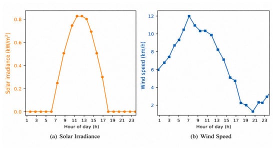
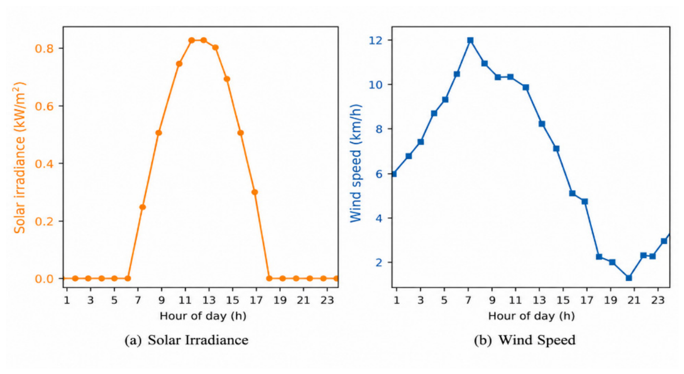
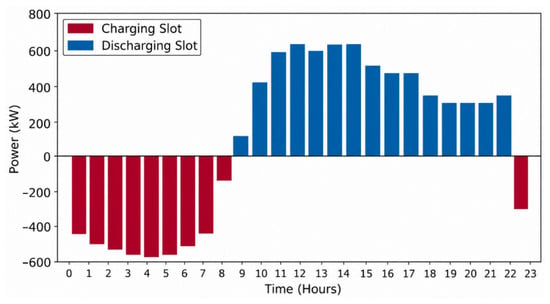
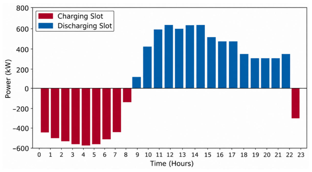
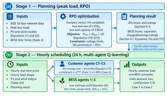
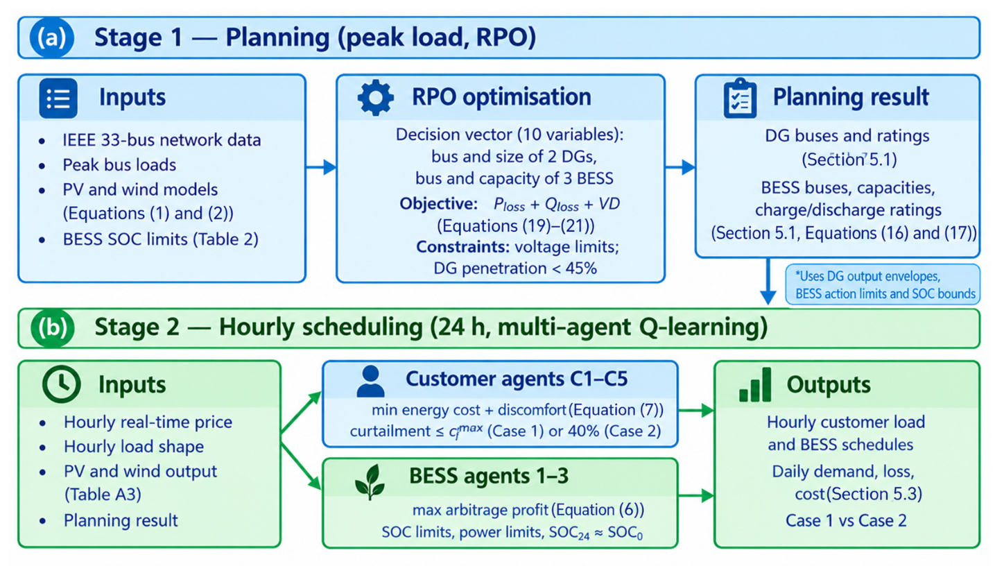
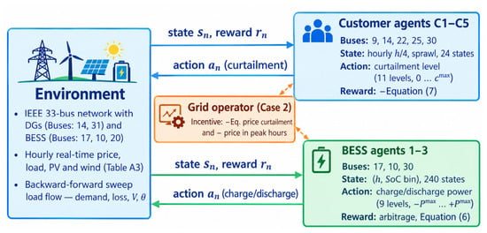
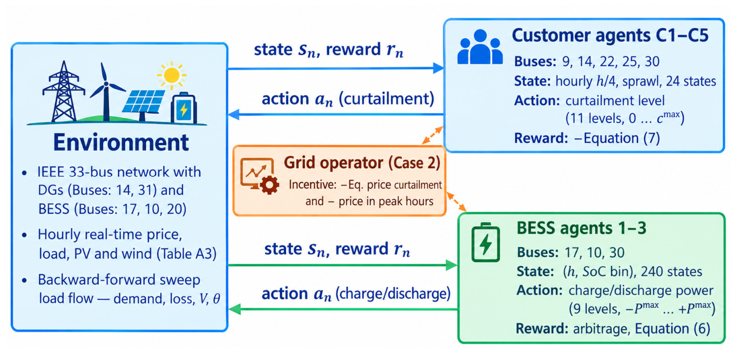
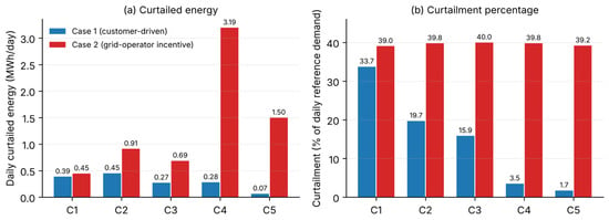
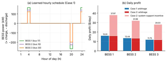
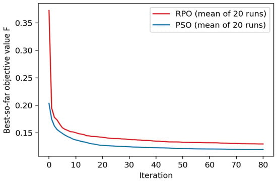
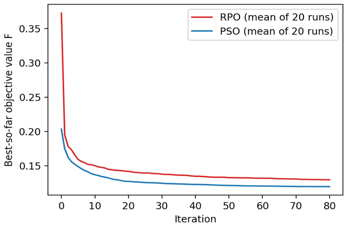
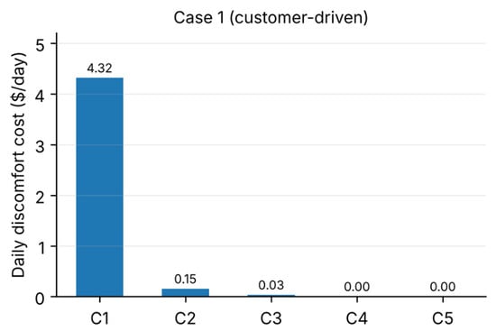
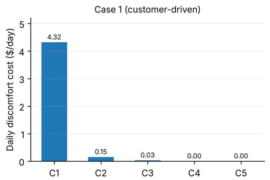
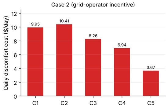
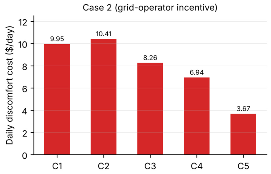
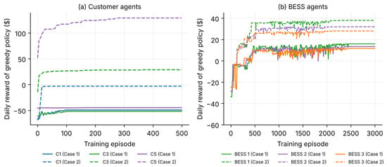
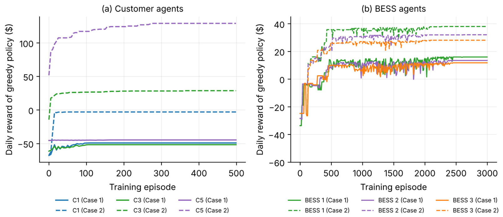

Disclaimer/Publisher’s Note: The statements, opinions and data contained in all publications are solely those of the individual author(s) and contributor(s) and not of MDPI and/or the editor(s). MDPI and/or the editor(s) disclaim responsibility for any injury to people or property resulting from any ideas, methods, instructions or products referred to in the content. |
© 2026 by the authors. Licensee MDPI, Basel, Switzerland. This article is an open access article distributed under the terms and conditions of the Creative Commons Attribution (CC BY) license.