Simultaneous Multiple Charging Stations Load Forecasting with Graph Neural Network

Abstract

Large-scale and stochastic electric vehicle (EV) charging behaviors pose challenges to the grid operation due to their spatial heterogeneity and temporal variability. This paper proposes a Multiple Charging Station (MCS) Collaborative Load Forecasting (MCSCLF) framework for simultaneous short-term forecasting of multiple charging stations. MCSCLF learns three latent inter-station graphs from short-term, daily and weekly charging-load views and couples them with view-specific spatiotemporal forecasting branches combining temporal convolution, graph convolution and attention features. The resulting multi-view features are fused for joint multi-station prediction. Experiments on real-world data from ten charging stations in Shenzhen demonstrate the ability of the proposed MCSCLF framework to jointly forecast station loads without a predefined spatial topology. Ablation studies show that the iterative graph refinement outperforms the tested fixed-graph and non-iterative alternatives, while the multi-scale temporal inputs and attention can further improve the forecasting accuracy within the proposed architecture.

1. Introduction

In order to address global climate change, more than 120 countries have pledged to achieve carbon neutrality [1], with the low-carbon transition of the automotive industry serving as an important pathway towards this goal [2,3]. As a special kind of load, EVs (electric vehicles) have random behaviors, i.e., selection of the charging station, charging time and charging patterns [4], which brings new challenges to the grid operation with random access of large-scale EVs [5], resulting in huge peak–valley differences [6]. Considering that the charging stations (CSs) are centralized charging places, it is necessary to predict the CS loads so as to pre-design the charging patterns and formulate specific charging strategies [7], i.e., locations and capacities of the CS [8] and orderly charging control strategies [9], thus maintaining grid-operation stability and further promoting the development of the EV industry.

CS load forecasting can be realized with historical data, mainly divided into traditional statistical methods (TSMs) [10] and deep learning methods (DLMs) [11]. The TSMs can model the load variations via statistically analyzing EV traveling patterns. More than one million charging transactions of 1700 CSs in four years are analyzed via clustering algorithms to identify the usage-related features for selecting CSs, including popularity, temporal characteristics, and user behaviors to assist in charging infrastructure planning and smart charging [12]. A bi-layer coordinated EV charging navigation framework is proposed which can jointly optimize the travel cost and grid-side energy interaction under transportation–distribution network coupling via dynamic energy estimation and V2G support [13]. With the application of the Monte Carlo simulation method [14], the weather-aware travel behavior and charging demand can be modeled to link the user travel modes, road traffic and environmental conditions to predict the spatiotemporal distribution of EV charging loads [15]. It should be noted that EV owners have a significant impact on the reliability of the load prediction model. A user-aware planning framework for residential EV charging stations is proposed with the integration of photovoltaic and energy storage, explicitly considering user response behavior and its uncertainty under both price-based and incentive-based demand response strategies to optimize the economic, environmental and operational performance [16].

An uncertainty framework for EV charging station load prediction is proposed with the integration of multidimensional spatiotemporal traffic flow forecasting [17], weighted quantile regression, and an enhanced queuing model to convert the traffic uncertainty into load uncertainty [18]. Further, a multi-agent deep reinforcement learning model is developed considering the optimization scheduling of CSs and regulation resources of the power grid in the data-driven training environment integrated with the Random Forest and grid-based EV mobility models, so as to provide day-ahead pricing and Nudge strategies with enhanced revenue and power curve tracking [19]. A hierarchical load forecasting model adaptable for different geographical regions is proposed [20], which is decomposed into several low-level standard probability models for solution, and the total load prediction can be obtained via the penalty linear quantile regression model with 9.5% higher prediction accuracy compared with those non-hierarchical methods. In summary, the load prediction accuracy of the TSM relies heavily on human experience, while different types of data are required for model validation, with poor generalization in various scenarios.

From the data-driven perspective, DLMs can alleviate certain limitations of the traditional statistical methods by learning forecasting patterns directly from data with less manual parameter specification. Shi et al. [21] proposed a stacking learning approach incorporating ensemble diversity regularization for load forecasting. For tempospatial network forecasting, Song et al. [22] developed STSGCN the to jointly capture the localized spatial–temporal correlations and model heterogeneity across different time periods. Three temporal networks, RNN (Recurrent Neural Network), LSTM (Long Short-Term Memory), and GRU (Gated Recurrent Unit), have been applied to bus charging-station load forecasting, with GRU achieving the best performance among the compared recurrent models [23]. Singular Spectrum Analysis (SSA) is used as an initial filter for noise removal, followed by an SSA-LSTM model for load forecasting [24]. A sequence-to-sequence (Seq2Seq) model has also been used to predict monthly charging loads of commercial EVs [25], demonstrating improved multi-step forecasting performance over the compared time-series models. Deep reinforcement Q-learning has also been applied to charging-load prediction under coordinated and uncoordinated charging scenarios [26].

More recently, the STDeepSeek [27] introduced a continual-learning-enhanced spatiotemporal large language model for EV charging-station load forecasting, highlighting the importance of adapting forecasting models to evolving charging patterns and newly observed data. This continual-learning perspective mainly addresses temporal and distributional adaptation of the forecasting model. In contrast, the present study focuses on how to infer and iteratively refine latent dependencies among multiple charging stations with structural adaption when no predefined station topology is available. However, most DLMs address load forecasting for a single CS using only temporal characteristics, without considering implicit inter-station dependencies or the spatial distribution of loads across multiple charging stations (MCS).

While extensive research exists on spatiotemporal load forecasting (e.g., traffic flow, weather), the MCS collaborative load forecasting (MCSCLF) solutions remain underexplored. The representative spatiotemporal forecasting models include JST-DHNet [28], which employs hierarchical synchronous learning modules to capture and fuse global and local spatiotemporal features. Additionally, a spatiotemporal dynamic network has been developed to model dynamic spatial similarity and periodic temporal shifts for taxi-flow prediction through gating and periodic-attention mechanisms [29].

Graph neural networks (GNNs) have powerful representation capabilities for non-Euclidean structured data, which can be applied for traffic flow prediction [30], where the spatiotemporal graph convolutional network (Ada-STGCN) is proposed with Wasserstein distance-based adversarial domain adaptation to accurately predict traffic flow in data-scarce target road networks by transferring knowledge from data-rich source networks. A traffic state prediction framework is developed that explicitly considers the spatiotemporal distribution and propagation of traffic over a road network by integrating a macroscopic traffic flow model, temporal–spatial dependency learning, graph-based interactions and data assimilation [31].

Although GNNs can offer advantages for spatiotemporal data, their reliance on predefined graph structures would often degrade the performance due to interference, i.e., missing relationships, redundancy and noise, hindering accurate feature learning. To address this, a novel feedback spatio–temporal GNN (FST-GNN) learning model is developed to predict the networked multi-agent formation states with noise interference [32]. Graph WaveNet [33] learns an adaptive dependency matrix through node embeddings and combines it with dilated temporal convolutions for spatial–temporal forecasting, which provides an established example of learning latent spatial dependencies from data. Related studies also investigate dynamic graph modeling for other spatial–temporal prediction tasks. A hierarchical spatiotemporal framework is designed for air-quality prediction [34] to capture short/long-term periodic features via dynamic graphs and attention, enhancing cross-domain adaptability. A BPF-GNN is proposed as the hierarchical graph feature extraction model with three-tier (Byte, Packet, Flow) graph structures to acquire multi-granularity information inherent in traffic, significantly improving the encrypted traffic classification accuracy [35]. In [36], a comprehensive analysis of 48 network measures in GNN-based stability assessments is conducted to improve the model generalization ability with only 20-node synthetic training datasets, which embodies the potential of GNN.

Although neural networks (CNNs, RNNs, GNNs) could offer solutions for spatiotemporal feature extraction in MCS load prediction, recent GNN-based temporal models often rely on predefined spatial relationships (i.e., road networks) or static graph structures, limiting their ability to capture complex, implicit interdependencies among charging stations. Different from continual-learning approaches that adapt forecasting models to newly arriving data, our work focuses on data-driven learning and refinement of latent inter-station relationships within the observed charging-station network. The key contributions of this paper are as follows.

• A multi-view collaborative forecasting formulation is developed for multiple charging stations without requiring a predefined physical or geographical graph. Different charging-load sequences are modeled jointly to characterize the temporal proximity, periodicity and longer-term tendency.
• An IDGL (Iterative Deep Graph Learning)-based graph structure learning module is adapted to the multi-charging station forecasting task. Three latent graphs are learned from short-term, daily and weekly load perspectives, respectively, allowing inter-station dependencies to be inferred from data.
• A view-specific spatiotemporal forecasting architecture is developed in which each learned graph is coupled with a corresponding forecasting branch. Each branch contains two spatiotemporal blocks with a temporal self-attention module between them, where the features from the three temporal views are fused for simultaneous multi-station forecasting.
• The integrated MCSCLF framework is evaluated on real-world charging-station data against temporal, graph-based and attention-based forecasting models, and controlled ablation experiments are performed to distinguish the effects of multi-scale temporal inputs, attention and graph construction, supporting the iterative refinement relative to the tested graph-based alternatives.

The remainder of the paper is organized as follows. Section 2 formulates the collaborative MCS load forecasting issue. Section 3 describes the detailed procedure of the graph network of the MCS with the IDGL-based graph structure learning module and the spatiotemporal feature extraction module. Numerical experiments are performed with the load dataset of a public CS in Shenzhen to verify the efficacy of MCSCLF in Section 4. The conclusion is provided in Section 5.

2. Problem Formulation

The load prediction of a single CS is only related to its own historical load, while urban MCS are distributed in different geographic regions with diversified spatial characteristics. Hence, the simultaneous load forecasting of MCS can be defined as a new class of spatiotemporal collaborative forecasting problem, i.e., the MCSCLF model. For instance, the load variation within the next H moments based on M historical load data can be expressed as,

$$\begin{array}{c}{\widehat{x}}_{t+1},\dots ,{\widehat{x}}_{t+H}=F_{\theta }(x_{t-M+1},\dots ,x_t)\hfill \end{array}$$

(1)

where $x_t=\left\{x_{t1},x_{t2},\cdots ,x_{tn}\right\}\in R^n$ is the load vector of MCS at t moment in n different locations, $F_{\theta }$ denotes the prediction model, and $\theta$ is the weight during training, i.e., mapping from historical sequence to the future sequence. The load forecasting of each CS in the region is not only related to the historical information of the CS itself, but also related to the historical loads of others.

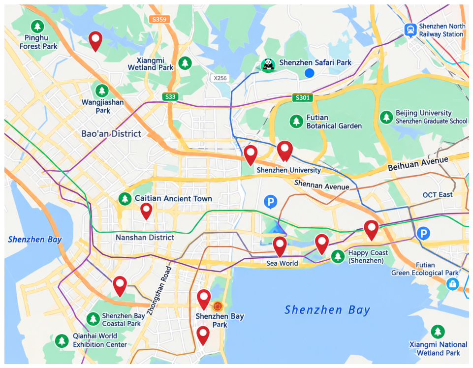
The MCS are distributed across different locations without an explicit predefined topology (see Figure 1), while collaborative forecasting requires the interactions among stations to be modeled. Conventional RNN- and CNN-based models do not explicitly encode such non-Euclidean inter-station relations, whereas graph-based models require a graph structure as relational input. Therefore, the implicit association among MCS can be modeled as a graph structure learning problem, i.e., to generate the graph structure based on the input data,

$$X_{in}\stackrel{\varphi }{\to }[X_{in},G]$$

(2)

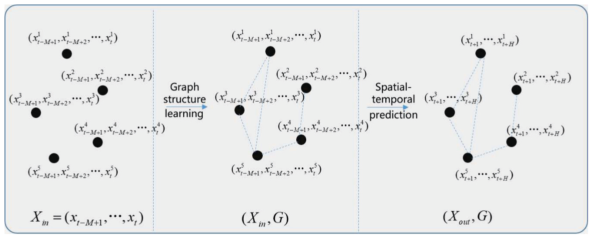
where the input data $X_{in}=(x_{t-M+1},\dots ,x_t)$ are the loads of M historical moments, $\varphi$ is the metric learning function; $G=(V,E)$ is the generated graph structure as described in Graph Theory, V is the set of graph nodes representing the CS, and E is the set of edges representing the implicit association among the MCS. Thus, the sequential load data of the MCS can be converted into graph data, as shown in Figure 2. The adjacency matrix of G is $A\in R^{N\times N}$, if $\{v_i,v_j\}\in V$ and $v_i,v_j\in E$, $A_{ij}\ne 0$ denotes the learned nonnegative edge weight, otherwise $A_{ij}=0$ indicating no connection. Based on the graph information, GNN can be applied for load forecasting,

$$[X_{in},G]\stackrel{f_{\theta }}{\to }[X_{out},G]$$

(3)

where $X_{out}=(x_{t+1},\dots ,x_{t+H})$ is the predicted output, f is the developed GNN model, and the subscript ${(·)}_{\theta }$ is the learning parameter vector.

Figure 1. The locations of the charging stations.

Figure 2. Modeling of the MCS collaborative load forecasting.

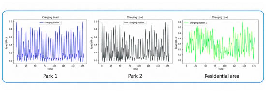
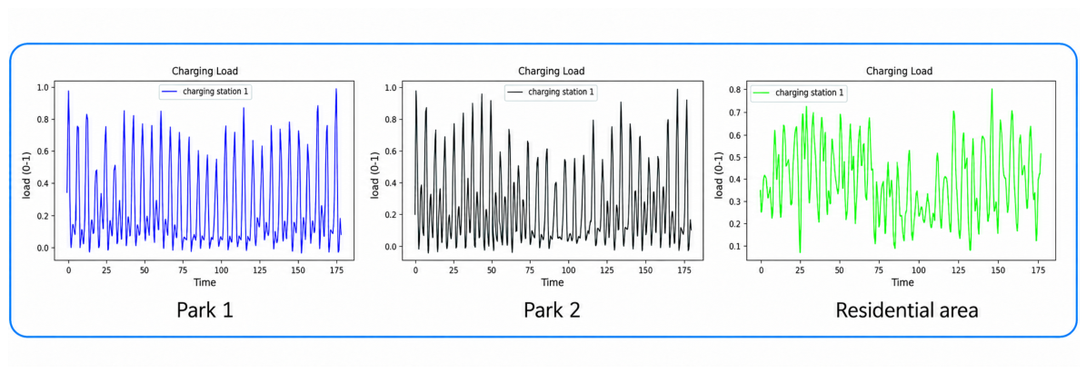
The loads of the MCS in three different urban areas within one month are displayed in Figure 3. It can be seen that the load variation of each CS has a strong temporal periodicity, where the load curves of the CS around Park1 and Park2 are more similar, but much different from that in the residential area. The reason is that the first two have relatively similar spatial properties, indicating that the MCS load variation characteristics are related to the spatial heterogeneity and periodicity. The MCS collaborative load prediction is discussed in the next Section.

Figure 3. The load variation curves of three CSs in Shenzhen.

3. Method of MCS Load Prediction

3.1. The Framework of the MCSCLF Model

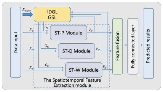
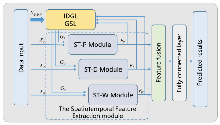
An end-to-end MCSCLF is proposed based on GCN (graph convolutional network), and it mainly includes two components, i.e., GSL (the graph structure learning) module and spatiotemporal feature extraction module (SFEM), as shown in Figure 4. At the data input layer, three types of MCS load data are input simultaneously, i.e., over a period of time, daily interval and weekly interval, written as $X=\{X_p,X_d,X_w\}\in R^{M\times N\times D}$; ${(·)}^M$ is the sequence length, ${(·)}^N$ is the node number of the MCS, and ${(·)}^D$ is the input dimension. In the GSL module, an implicit graph structure among the MCS nodes can be generated based on each input data, i.e., $G=\{G_p,G_d,G_w\}$ generated from the input vector X, where G is iteratively updated in the process of spatiotemporal feature extraction. The SFEM is divided into three sub-modules, $\{ST-P,ST-D,ST-W\}$ (Period, Day, Week) for the three types of input, respectively, sharing the same structure to extract the temporal proximity features, periodic features and tendency features of the MCS load. Finally, the three temporally conditioned latent graphs with the corresponding spatiotemporal features are integrated in the fully connected layer (FCL) for the collaborative MCS final load prediction.

Figure 4. The framework of the MCSCLF model.

3.2. IDGL-Based GSL Module

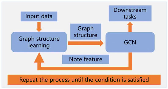
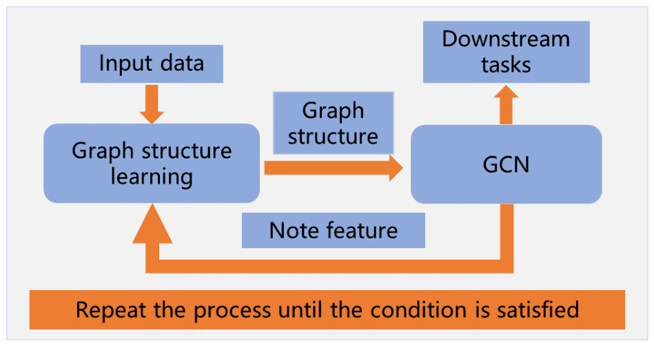
In the GSL module, the Iterative Deep Graph Learning (IDGL) model [37] is applied to learn both the graph structure and the GCN parameters iteratively. Hence, the alternating update rule, weighted cosine similarity, multi-head similarity aggregation, and graph regularization in Equations (4)–(13) are inherited from the IDGL formulation. The task-specific adaptation in this work is to apply this learning process separately to $X_p$, $X_d$ and $X_w$, thereby obtaining three temporally conditioned charging-station graphs $G_p$, $G_d$ and $G_w$, which are subsequently coupled with the corresponding ST-P, ST-D, and ST-W forecasting branches. As originally proposed in IDGL [37], the alternating procedure uses the updated node representations to refine the graph and subsequently uses the refined graph to update the node representations, depicted in Figure 5. The IDGL involves two alternating iterations, (1) GSL: Update the adjacency matrix $A\left(t\right)$ via the current node features $X\left(t\right)$; (2) GCN Feature Learning: Update the node features $X(t+1)$ via the current graph $A\left(t\right)$, which can be described mathematically,

$$\left\{\begin{array}{c}{A}^{\left(t\right)}=\underset{A}{argmin}\left(L_{task}+L_g\left(A,X^{\left(t\right)}\right)\right)\left(Structureupdate\right)\\ X^{\left(t+1\right)}=GCN\left(A^{\left(t\right)},X^{\left(t\right)}\right)\left(Featureupdate\right)\end{array}\right.$$

(4)

where t denotes the iteration step.

Figure 5. The framework of the IDGL.

All nodes (CS) are treated as homogeneous peers without prior topological knowledge, and the constructed graph is assumed to be undirected and symmetric, i.e., $A_{i,j}=A_{j,i}$. For each forecasting sample, the graph construction is based only on the historical input observations available to the model. Future target values $X_{t+1},\dots ,X_{t+H}$ are not used for similarity computation or graph refinement. It should be noted that the proposed optimization is an alternating graph-learning procedure rather than a metaheuristic population-based optimizer. Compared with constructing a graph only from the original node features, the alternating procedure uses updated GCN representations to refine the graph and then uses the refined graph for subsequent feature updates. Accordingly, the iterative graph-refinement mechanism itself is inherited from IDGL rather than introduced as a new graph-learning algorithm. The task-specific adaptation of MCSCLF lies in applying this mechanism separately to the short-term, daily, and weekly charging-load views and coupling the resulting graphs with the corresponding spatiotemporal forecasting branches.

In order to learn the hidden relationship of MCS nodes, a graph similarity metric learning method is applied to design the cosine similarity as the metric function,

$$s_{ij}=\cos (w⨀x_i,w⨀x_j)$$

(5)

where ⨀ denotes the Hadamard product, w is the learnable parameters and $\{x_i,x_j\}$ are the input data.

The criteria for establishing and updating graph structures among MCS are as follows. Each similarity can be considered as part of the semantic features of the vectors with multi-head aggregation. In order to improve the expression capability, the cosine similarity is extended to a multi-head version via m weight vectors, i.e., the multiple independent similarity matrices are calculated separately, and the mean is taken as the final similarity,

$$s_{ij}^p=\cos ({\omega }_p⨀x_i,{\omega }_p⨀x_j)$$

(6)

$$s_{ij}={\displaystyle \frac{1}{m}}{\displaystyle \sum _{p=1}^m}{s}_{ij}^p$$

(7)

where ${\omega }_p$ is the learnable weight vector for head p; $s_{ij}^p$ is used to compute the $p^{th}$ cosine similarity of the input feature vectors $x_i$ and $x_j$, representing partial vector semantic feature. Then, the adjacency matrix A is configured by the calculated similarities of all nodes to complete the GSL. For each temporal view, the historical input window is flattened into a feature vector for each station. An IDGL-based module alternates between the adjacency construction and node-feature updates using its own GCN. The resulting adjacency matrix is then supplied to the corresponding spatiotemporal forecasting branch, but the branch output is not fed back into the graph learner during the forward pass. The graph learner and forecasting branch are jointly trained through back-propagation mode. The overall training procedure of MCSCLF is summarized in Algorithm 1. Negative retained similarities are truncated to zero using

$${\overline{A}}_{ij}=\max (s_{ij},0).$$

(8)

The adjacency matrix is subsequently symmetrized according to

$$A={\displaystyle \frac{1}{2}}\left(\overline{A}+{\overline{A}}^T\right),$$

(9)

and its diagonal entries are set to zero. Before graph convolution, self-loops are added, and the adjacency matrix is normalized as

$$\tilde{A}=A+I,\widehat{A}={\tilde{D}}^{-1/2}\tilde{A}{\tilde{D}}^{-1/2}.$$

(10)

Algorithm 1 Training procedure of MCSCLF

Require: Training samples $\{X_p,X_d,X_w,Y\}$; maximum refinement iterations $R=2$; convergence tolerance ${ϵ}_g={10}^{-3}$; hyperparameters $\lambda ,\alpha ,\beta ,\gamma$ Ensure: Trained model parameters $\mathsf{\Theta }$   1:  for each training mini-batch do   2:        for $v\in \{p,d,w\}$ do   3:              Extract view-specific input features $X_v$   4:              Compute pairwise weighted cosine similarities using Equations (5)–(7)   5:              Retain the top-5 similarities, apply ReLU, symmetrize the adjacency matrix, and set its diagonal to zero to obtain $A_v^{\left(0\right)}$   6:              for $t=0$ to $R-1$ do   7:                    Update node representations using $H_v^{(t+1)}=\mathrm{GCN}(A_v^{\left(t\right)},H_v^{\left(t\right)})$   8:                    Recompute pairwise similarities from $H_v^{(t+1)}$   9:                    Retain top-5 similarities, apply ReLU, symmetrize, and set the diagonal to zero to obtain $A_v^{(t+1)}$ 10:                    if $t\ge 1$ and ${\displaystyle \frac{\parallel A_v^{(t+1)}-A_v^{\left(t\right)}{\parallel }_F}{\parallel A_v^{\left(t\right)}{\parallel }_F}}<{ϵ}_g$ then 11:                          break 12:                    end if 13:              end for 14:              Extract spatiotemporal feature $F_v$ using the corresponding ST branch 15:        end for 16:        Fuse $F_p$, $F_d$, and $F_w$ 17:        Compute the multi-step prediction $\widehat{Y}$ 18:        Compute the joint loss using Equation (27) 19:        Update trainable parameters by back-propagation 20:  end for

As summarized in Algorithm 2, the model parameters remain fixed during the inference, whereas $G_p$, $G_d$ and $G_w$ are reconstructed and iteratively refined for each new forecasting window according to its input features. Hence, the graph adaptation is input-dependent structural inference rather than online parameter updating or continual learning.

Algorithm 2 Inference procedure of MCSCLF

Require: New input window $\{X_p,X_d,X_w\}$; trained parameters $\mathsf{\Theta }$; maximum graph iterations $R=2$; tolerance ${ϵ}_g={10}^{-3}$ Ensure: Multi-step prediction $\widehat{Y}$   1:  Fix all trained parameters $\mathsf{\Theta }$   2:  for $v\in \{p,d,w\}$ do   3:        Compute weighted cosine similarities from $X_v$   4:        Retain top-5 similarities, apply ReLU, symmetrize, and set diagonal to zero   5:        for $t=0$ to $R-1$ do   6:              Update node representations using graph convolution   7:              Recompute the input-dependent adjacency matrix   8:              if relative adjacency change $<{ϵ}_g$ then   9:                    break 10:              end if 11:       end for 12:       Extract feature $F_v$ with the corresponding ST branch 13:  end for 14:  Fuse $F_p,F_d,F_w$ and compute $\widehat{Y}$

The graph regularization method is further applied to improve the smoothness, connectivity and sparsity of the graph structure to guarantee the quality of the acquired graph structure. The smoothness refers to smooth variation of the graph signals among the neighboring nodes. Given the symmetric weight matrix A of the undirected graph, the smoothness $\mathsf{\Omega }(A,X)$ of the graph signals $x_1,\dots ,x_n\in R^d$ can be measured by the Dirichlet energy,

$$\mathsf{\Omega }(A,X)={\displaystyle \frac{1}{2n^2}}\sum _{i,j}{A}_{ij}{\parallel x_i-x_j\parallel }_2^2={\displaystyle \frac{1}{n^2}}\mathrm{tr}\left(X^{T}LX\right)$$

(11)

where L is the graph Laplacian matrix, $D_{ii}={\sum }_j{A}_{ij}$ is the degree matrix. Minimizing $\mathsf{\Omega }(A,X)$ encourages neighboring nodes to have similar features, thereby promoting the smoothness of the graph signals. The graph sparsity $f\left(A\right)$ is written as,

$$f\left(A\right)={\displaystyle \frac{-\beta }{n}}{I}^T\log \left(AI\right)+{\displaystyle \frac{\gamma }{n^2}}{\left|\right|A\left|\right|}_F^2$$

(12)

where ${∥·∥}_F$ is the Frobenius norm, $\beta$ and $\gamma$ are the non-negative hyperparameters. The first item on the right side of Equation (12) is used to avoid the non-connected graph formation, and the second item is used to reduce the node degree to control the graph sparsity. The overall regularization loss of the graph can be obtained by summing the smoothness loss and the sparse constraint loss,

$$L_g=\alpha \mathsf{\Omega }(A,X)+f\left(A\right)$$

(13)

where $\alpha$ is a non-negative hyperparameter. The graph regularization term $L_g$ is used to encourage the desired smoothness, connectivity, and sparsity properties during the optimization. For the final reported experiments, the validation-selected graph-learning configuration is $\lambda =0.99$, $\alpha =1$, $\beta =0$ and $\gamma =1$, with a maximum of $R=2$ graph-refinement iterations. These values are fixed before final test evaluation. With $\beta =0$, the connectivity-preserving regularization term is inactive and contributes neither to the loss nor to its gradients. Only the smoothness and Frobenius-norm penalty terms remain active in the graph regularization.

3.3. GCN and TCN Based SFEM

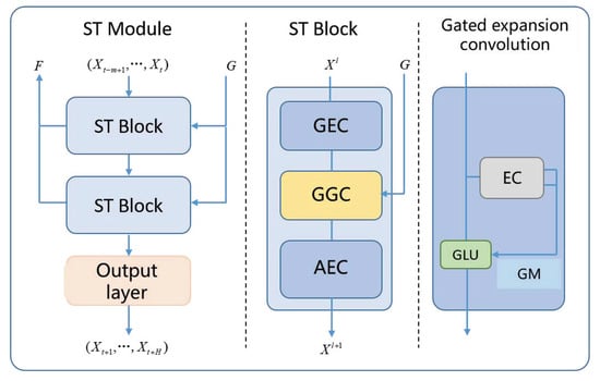
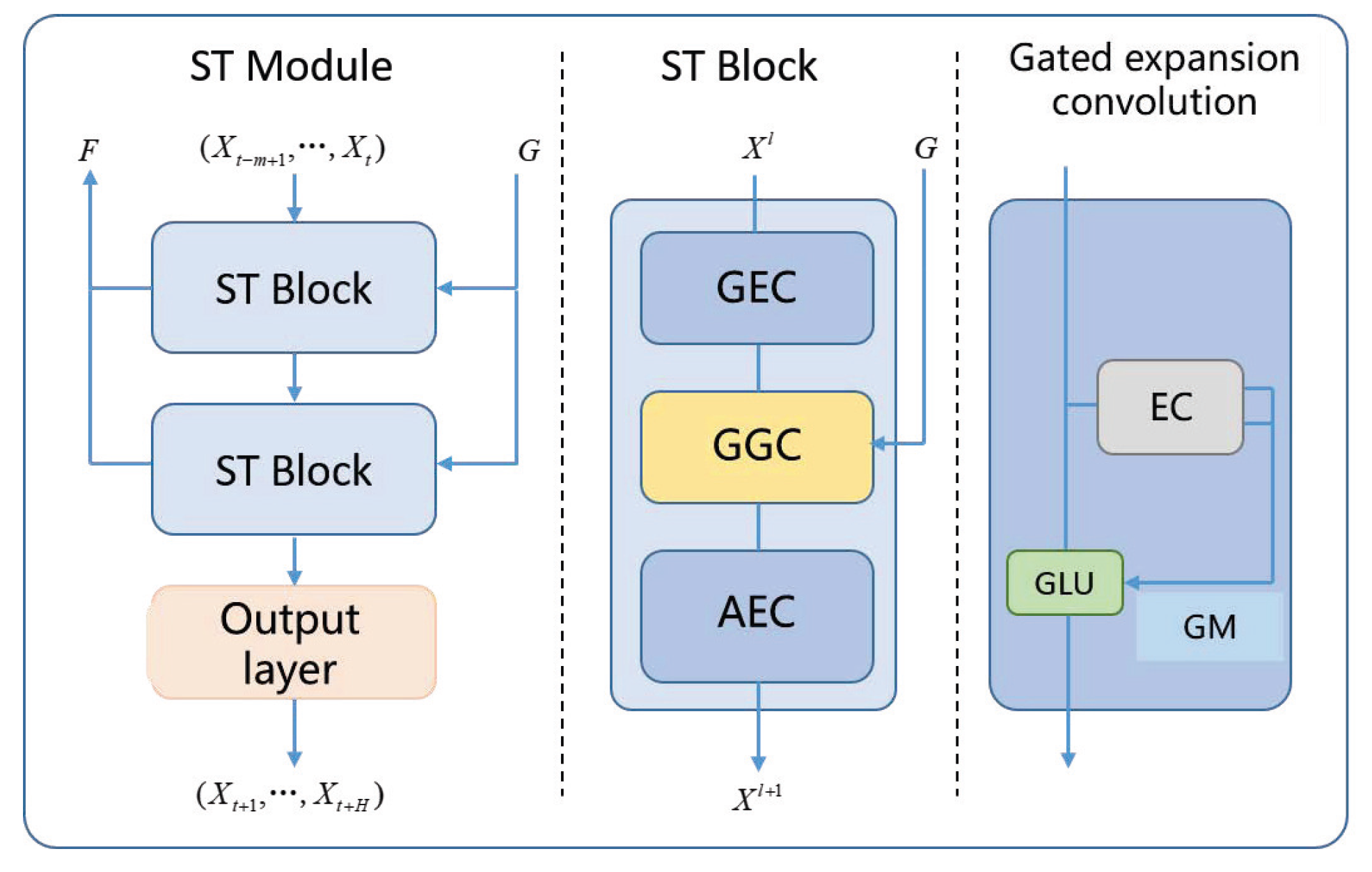
The SFEM is constructed based on graph convolution and temporal convolution, as illustrated in Figure 6. The ST-P, ST-D and ST-W branches share the same network architecture. Each ST module consists of two ST sub-blocks. The basic temporal graph–temporal organization is inspired by the sandwich-like structure of STGCN [38], whereas the internal temporal modeling is modified for the present forecasting task. Specifically, each ST sub-block consists of a Gated Expanded Convolution (GEC) layer, a Gated Graph Convolution (GGC) layer, and an Attention Expanded Convolution (AEC) layer. The GEC layer captures local temporal dynamics through gated dilated convolution, the GGC layer models spatial dependencies among charging stations using the learned graph, and the AEC layer further captures adaptive and longer-range temporal dependencies through self-attention and dilated convolution. Therefore, the proposed ST sub-block is not a direct reproduction of the standard STGCN block but a task-specific extension for MCS load forecasting.

Figure 6. The framework of the SFE module.

The graph-convolution layer propagates spatial information according to the learned graph. The temporal–graph–temporal organization forms a bottleneck-style block around graph convolution for compact feature transformation. Here, G denotes the learned graph used by each ST sub-block, and F denotes the extracted spatiotemporal feature that is fed back to the GSL module during iterative graph refinement.

Although the recurrent neural networks (i.e., RNN, GRU, and LSTM) have achieved satisfactory results in time-series analysis, their sequential computation can limit parallelism and increase training time. The function of TCN (Temporal Convolutional Network) is to model the short-term dynamic evolution of the load rather than static average behavior, which has the advantages of fast training speed, simple structure and no dependency constraints between computational steps. Hence, the GEC is adopted in the ST sub-block to extract the time-series dynamic features of the load variation,

$$H^{\prime }=Dil\_Con{v}_f\left(X^l\right)=f\ast {\mathrm{H}}^l$$

(14)

where $H^l\in R^{M\times N\times C_i}$ is the $l^{th}$ layer input, $Dil\_Conv$ is the dilated convolution, $f\in R^{K\times 2C_o}$ is the convolution kernel; $H^{\prime }\in R^{(M-K+1)\times N\times 2C_o}$ is the output, ${(·)}^N$ is the node number of MCS, ${(·)}^M$ is the length of the load variation sequence, ${(·)}^K$ is the convolution kernel size, and ${(·)}^{\left\{C_i\right\}}$ & ${(·)}^{\left\{C_o\right\}}$ are the numbers of the input and output channels, respectively. $H^{\prime }$ is then split equally, and the gated linear units (GLUs) are used to increase the nonlinearity,

$$(H_1^{\prime },H_2^{\prime })=split\left(H^{\prime }\right)$$

(15)

$$H^{l_1}=H_1^{\prime }\ast \tau H_2^{\prime }=\tanh \left(H_1^{\prime }\right)\ast \mathrm{sigmoid}\left(H_2^{\prime }\right)$$

(16)

where $split$ denotes the splitting operation, $(H_1^{\prime },H_2^{\prime })\in R^{(M-K+1)\times N\times C_o}$ is the gated input vector, $H^{l_1}\in R^{(M-K+1)\times N\times C_o}$ is the output, and $\{\tanh ,\mathrm{sigmoid}\}$ are the activation functions. In the GGC layer, the first-order approximate GCN is embedded into the temporal gating unit to extract the spatial and local temporal features simultaneously, which are described as,

$$\theta \ast g{H}^l=\theta ({\tilde{D}}^{-{\displaystyle \frac{1}{2}}}\tilde{A}{\tilde{D}}^{-{\displaystyle \frac{1}{2}}})H^l$$

(17)

$$(H_1^{\prime },H_2^{\prime })=split(\theta \ast g{H}^l)$$

(18)

$$H^{l_2}=H_1^{\prime }\ast \tau H_2^{\prime }=\tanh \left(H_1^{\prime }\right)\ast sigmoid\left(H_2^{\prime }\right)$$

(19)

where $\ast g$ is the graph convolution operation, $\theta \in R^{K\times C_i\times C_o}$ is the learnable parameter, $\{{\tilde{D}}^{-{\displaystyle \frac{1}{2}}},\tilde{A}\}$ are the prior information obtained from the graph structure G,

$$\tilde{A}=A+I$$

(20)

$${\tilde{D}}_{ii}={\sum }_j{\tilde{A}}_{ij}$$

(21)

$A\in R^{N\times N}$ is the adjacency matrix of the graph G, and $\tilde{D}\in R^{N\times N}$ is the degree matrix. In the gated attention-inflated convolutional layer, the global temporal features are further extracted, while a self-attentive mechanism is introduced in order to capture the temporal dynamic properties, i.e., different sequence inputs may have varied temporal dependencies,

$$(Q,K,V)=H^{l_2}(w_Q,w_K,w_V)$$

(22)

$$Att(Q,K,V)=\mathrm{softmax}\left({\displaystyle \frac{Q{K}^T}{\sqrt{C_i}}}\right)V$$

(23)

$$H^{l+1}=Dil\_Con{v}_f\left(Att(Q,K,V)\right)=f\ast Att(Q,K,V)$$

(24)

where $\{Q,K,V\}$ are the query, key and value matrices, $\{w_Q,w_K,w_V\}$ are the learnable parameters, $Att$ is the attention calculation function, and $H^{l+1}$ is the $l^{th}$ layer output.

3.4. Model Training

The temporal features $\{H_p^o,H_d^o,H_w^o\}$ extracted from the ST-P, ST-D and ST-W modules are stitched together as $H_{all}^o$, so that $H_{all}^o$ contains all the temporal proximity features, periodic features and trend features of the load variations. Then they are input into the FCL to calculate the final prediction,

$${[X_{t+1},\dots ,X_{t+H}]}_{pred}=\tanh (W_p{H}_{all}^o+b_p)$$

(25)

where $W_p$ and $b_p$ are the learnable parameters. In this paper, the mean absolute error (MAE) is used as the loss function of the load prediction,

$$L_{\mathrm{pred}}={\displaystyle \frac{1}{HN}}{\displaystyle \sum _{h=1}^H}{\displaystyle \sum _{j=1}^N}\left|{\widehat{X}}_{t+h,j}-X_{t+h,j}\right|$$

(26)

Since the GSL is performed iteratively in the process of the SFE, the comprehensive joint loss function of the GSL and the load prediction is defined as,

$$L=\lambda L_{\mathrm{pred}}+(1-\lambda )L_g$$

(27)

where $\lambda \in [0,1]$ balances the forecasting loss and the graph-regularization loss. A larger $\lambda$ places greater emphasis on the forecasting accuracy, whereas a smaller $\lambda$ increases the influence of the graph regularization. Within $L_g$, $\alpha$ weights the graph-smoothness term, $\beta$ weights the connectivity-preserving term, which penalizes small node degrees when active and is disabled in the final reported configuration as $\beta =0$, and $\gamma$ controls the Frobenius-norm penalty on the adjacency matrix and hence the sparsity of the learned graph. By optimizing this loss function, the overall training of the model can be achieved, and the model parameters can be determined while learning the optimal graph structure.

4. Experiment and Result Analysis

4.1. Experimental Settings

A real-world dataset (seen in Figure 1), denoted as SzCS1, is configured with the charging load data of 10 randomly selected public CS in Shenzhen, as Shenzhen is one of the first pilot cities of EV deployment in China. The aligned dataset contains 10 min charging-energy observations from 19 August to 19 November 2020. The data are divided into three non-overlapping subsets, from 19 August to 19 October for training, from 20 October to 3 November for validation and model selection, and from 4 November to 19 November for final test, i.e., 7906 training, 2158 validation, and 2302 test.

The Min–Max normalization parameters are estimated separately for each station using training-period observations only and are then fixed and applied unchanged to the validation and test data. No temporal shuffling is performed across the three subsets. The aligned 10 min dataset contains no missing values, and no missing-value imputation was performed. The data-loading routine checks for missing values and irregular timestamp intervals and rejects inputs that fail these checks. Outlier correction uses linear interpolation between neighboring valid observations within the same chronological subset, without crossing subset boundaries. Only one training-period observation, at station 345 on 29 September 2020, required correction; no validation or test observations are replaced, and neither period is used to correct the training data. The outlier-detection thresholds and the Min–Max normalization parameters are estimated via the training-period observations only and are then fixed and applied to the validation and test data.

All formal experiments are implemented using PyTorch 2.4.1 with CUDA 12.1 and cuDNN 9.1 on an NVIDIA RTX 3090 Ti GPU. The model uses the previous 120 min of data to predict the next 30 min, i.e., 12 ($M=12$) historical points are used to predict 3 ($H=3$) future points. The final experiments retain both weekdays and weekends. For all models, the optimizer is Adam with batch size 256, weight decay ${10}^{-6}$, gradient clipping at 5, and a maximum of 100 epochs. Validation MAE is used for early stopping with patience 15 and for best-checkpoint selection. The learning rate is adjusted by ReduceLROnPlateau with factor 0.5 and patience 5. The common training settings are summarized in Table 1.

Table 1. The experimental training settings.

Parameter	Value
Optimizer	Adam
Batch size	256
Weight decay	${10}^{-6}$
Gradient clipping	5
Maximum epochs	100
Early stopping	validation MAE, patience 15
Learning-rate scheduler	ReduceLROnPlateau, factor 0.5, patience 5
Final random seeds	41, 42, 43

The MAE and RMSE (root mean square error) are used as evaluation criteria,

$$\begin{array}{c}\mathrm{MAE}={\displaystyle \frac{1}{m}}{\displaystyle \sum _{i=1}^m}|y_{test}^{\left(i\right)}-{\widehat{y}}_{test}^{\left(i\right)}|\hfill \end{array}$$

(28)

$$RMSE=\sqrt{{\displaystyle \frac{1}{m}}\sum _{i=1}^m{\left(y_{\mathrm{test}}^{\left(i\right)}-{\widehat{y}}_{\mathrm{test}}^{\left(i\right)}\right)}^2}$$

(29)

where $y_{test}^{\left(i\right)}$ and ${\widehat{y}}_{test}^{\left(i\right)}$ denote the ground-truth and predicted values of the $i^{th}$ test sample, respectively, and m is the number of evaluated prediction elements.

Four benchmark models are considered: MLP, LSTM [39], Transformer [40], and DCRNN [41]. All models use the same 10 charging stations, chronological split, training-only normalization, short-term/daily/weekly input views, 12-step historical window, 3-step forecasting horizon, and joint $N\times H$ output. To ensure comparable hyperparameter-selection effort, eight candidate configurations are predefined for each model. Candidate selection uses seed 42 and validation MAE only, without test evaluation. The selected configuration is subsequently retrained and evaluated using seeds 41, 42, and 43, and the final baseline and ablation results are reported as mean ± sample standard deviation. The eight MCSCLF candidate configurations and their validation MAEs are listed in Table 2. Candidate 2 yields the lowest validation MAE with seed 42 and iss fixed for the final three-seed experiments. The subsequent sensitivity analysis is conducted separately and is not used to revise this selection. The validation-selected configurations of all compared models are summarized in Table 3.

Table 2. Predefined MCSCLF candidate configurations and validation results.

Candidate	Hidden Dim.	R	Learning Rate	$\mathit{\lambda }$	$\mathit{\alpha }$	$\mathit{\beta }$	$\mathit{\gamma }$	Val. MAE (kWh)
1	64	3	${10}^{-3}$	0.90	0.10	0.10	0.10	9.6976
2	64	2	${10}^{-3}$	0.99	1.00	0	1.00	6.6944
3	32	2	${10}^{-3}$	0.90	0.10	0.10	0.10	9.4505
4	32	2	$3\times {10}^{-4}$	0.99	0.10	0.10	0.10	8.2082
5	32	3	${10}^{-3}$	0.90	0.01	0.10	0.10	9.8871
6	32	3	$3\times {10}^{-4}$	0.90	0.10	0.01	0.10	9.8942
7	64	2	$3\times {10}^{-4}$	0.70	0.10	0.10	0.10	9.4409
8	64	3	$3\times {10}^{-4}$	0.90	0.10	1.00	0.10	10.4982

Notes: All candidates use seed 42 and the same chronological data split. Hidden and output feature dimensions are equal. Other settings are held fixed. Selection use the validation MAE only, without test-set evaluation. Candidate 2 is selected.

Table 3. Validation-selected configurations of the comparison models.

Model	Configuration
MLP	2 hidden FC layers; hidden width 128; ReLU; dropout 0; learning rate ${10}^{-3}$
LSTM	1 LSTM layer; hidden size 64; dropout 0; learning rate ${10}^{-3}$
DCRNN	2 DCGRU layers; hidden size 64; forward/backward diffusion steps 2; dropout 0.1; learning rate ${10}^{-3}$; training-data Pearson-correlation graph with top-$k=5$ and symmetrization
Transformer	2 encoder layers; $d_{\mathrm{model}}=64$; 4 heads; FFN = 128; dropout 0.1; learning rate ${10}^{-3}$
MCSCLF	Three 64-dimensional temporal-view branches; temporal kernel 3; dilations 1 and 2; 2 attention heads; 8 weighted-cosine heads; top-$k=5$; $R=2$; dropout 0.1; learning rate ${10}^{-3}$; $\lambda =0.99$, $\alpha =1$, $\beta =0$, $\gamma =1$

4.2. Experimental Results and Analysis

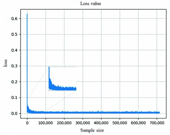
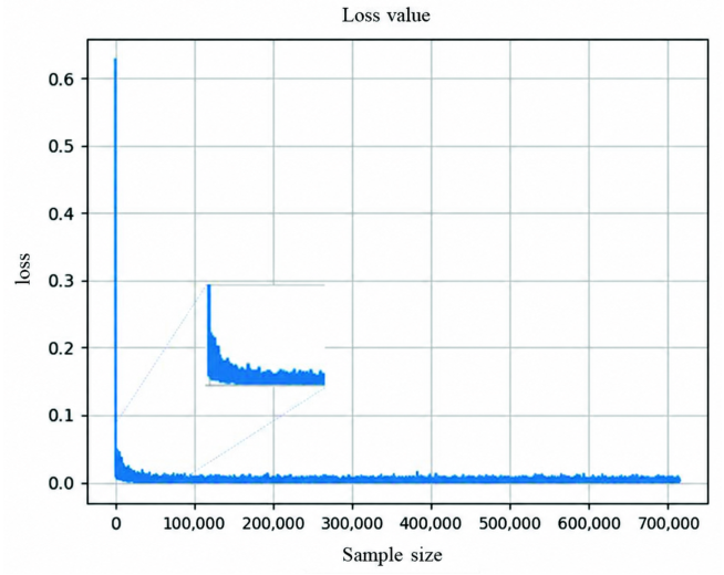
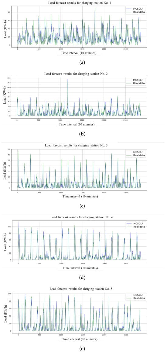
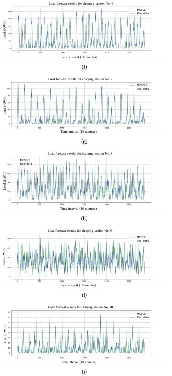
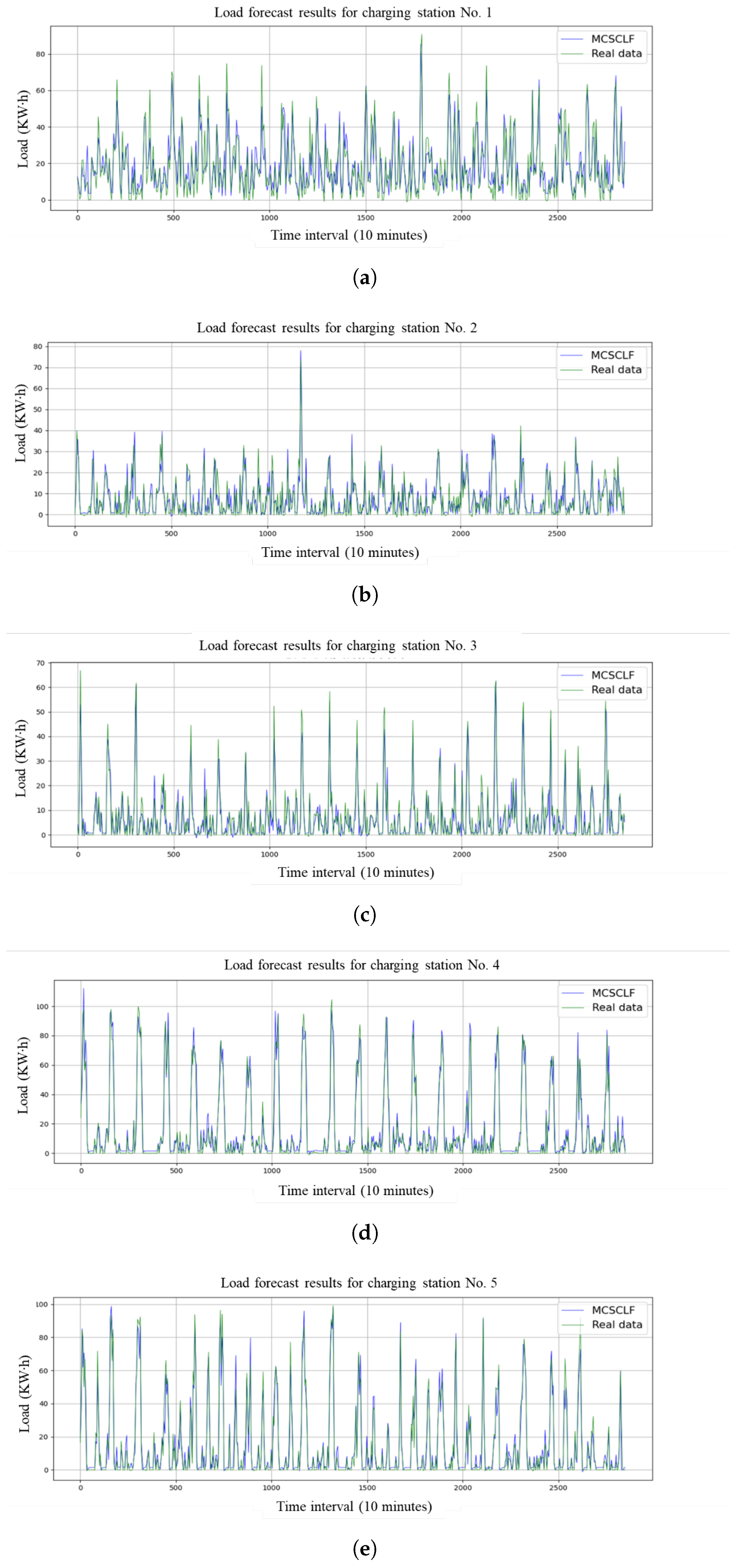
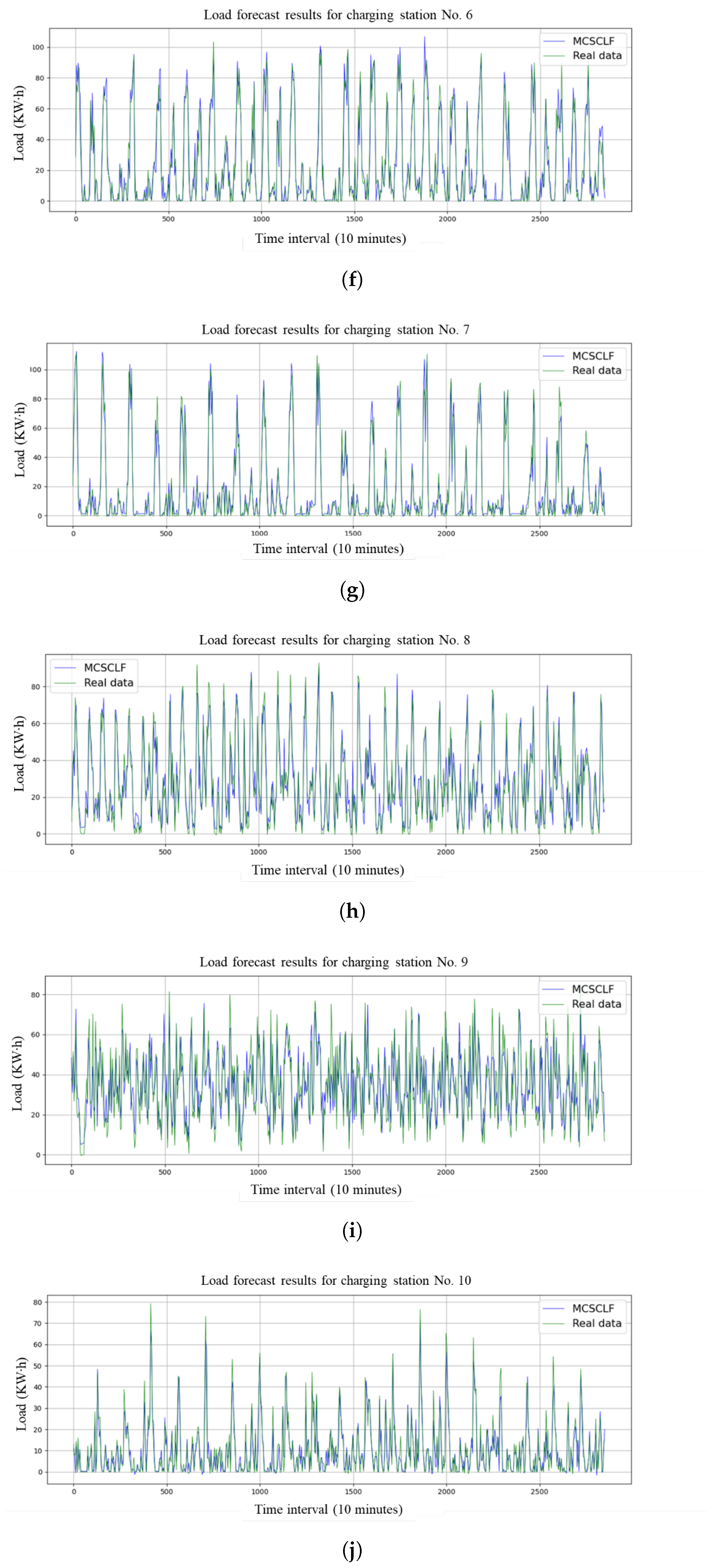
Figure 7 shows a representative training-loss curve of the MCSCLF model. Representative load-prediction results for the final chronological test period (4–19 November 2020) are demonstrated in Figure 8. It can be seen that the predicted charging energy closely follows the measured charging energy, indicating that the developed model can extract different spatiotemporal characteristics of MCS and provide effective multi-station forecasts under the evaluated setting. Specifically, the model captures three types of dynamic temporal features, namely temporal proximity, periodicity and tendency, by jointly modeling the load sequences over different time scales. The temporal proximity features reflect short-term load evolution in adjacent time intervals, the periodic features describe recurrent daily charging patterns, and the tendency features characterize longer-term variation trends.

Figure 7. Representative training-loss variation of the MCSCLF model.

Figure 8. (a–e) MCSCLF model prediction results for charging stations 1–5; (f–j) MCSCLF model prediction results (continued) for charging stations 6–10.

Thanks to the introduction of the dilated convolution in the TCN module, the developed MCSCLF model can effectively enlarge the temporal receptive field without significantly increasing the network depth, so that both short-term fluctuations and relatively long-range temporal dependencies can be captured simultaneously. As a result, the model can respond more quickly to dynamic load changes and better track rapid variations, rather than relying excessively on historical average behaviors as in many recurrent forecasting models. As shown in Figure 8a–c, the proposed model can follow short-term dynamic fluctuations with satisfactory accuracy. Moreover, in Figure 8c–f, the load curves exhibit obvious periodic variation characteristics, and the prediction results remain close to the actual values, further demonstrating that the proposed model can effectively capture the dynamic temporal evolution of MCS loads under different operating patterns.

The final fair-comparison results are summarized in Table 4. DCRNN achieves the lowest overall MAE and RMSE, $5.9810\pm 0.0227$ kWh and $9.6245\pm 0.0495$ kWh, respectively. MCSCLF obtains $6.4680\pm 0.1567$ kWh MAE and $10.5598\pm 0.2250$ kWh RMSE. Its MAE is approximately 0.85% lower than that of the MLP, but its RMSE is higher than those of all four baselines, and its across-seed variability is the largest among the compared models. Therefore, MCSCLF is interpreted as providing competitive joint multi-station forecasting performance rather than uniformly superior accuracy.

Table 4. Overall forecasting performance under the fair joint multi-station protocol.

Model	Test MAE (kWh)	Test RMSE (kWh)
MLP	$6.5236\pm 0.0368$	$9.9628\pm 0.0525$
LSTM	$6.0838\pm 0.0082$	$9.6860\pm 0.0261$
DCRNN	$\mathbf{5.9810}\pm \mathbf{0.0227}$	$\mathbf{9.6245}\pm \mathbf{0.0495}$
Transformer	$6.1322\pm 0.0477$	$9.6811\pm 0.0946$
MCSCLF	$6.4680\pm 0.1567$	$10.5598\pm 0.2250$

The station-level results in Table 5 are consistent with the overall ranking and indicate that the performance differences are not driven by a single charging station. Stations 345 and 382 are relatively difficult for all models.

Table 5. Per-station forecasting results (MAE/RMSE in kWh).

Model	122	345	346	347	348	349	360	361	372	382
MLP	7.635/10.264	10.585/15.260	3.976/5.828	3.581/6.474	5.022/8.178	5.102/8.722	6.956/10.131	5.340/8.590	7.715/10.305	9.322/12.352
LSTM	7.408/10.346	9.618/14.913	3.627/5.549	3.452/6.583	4.506/7.542	4.422/7.919	6.614/10.019	4.868/8.067	7.501/10.189	8.823/12.067
DCRNN	7.226/10.084	9.841/15.245	3.641/5.796	3.405/6.277	4.330/7.399	4.057/7.702	6.463/9.997	4.790/8.097	7.373/10.116	8.686/11.717
Transformer	7.435/10.228	9.778/15.038	3.682/5.589	3.532/6.614	4.486/7.389	4.479/7.982	6.659/10.049	4.893/8.112	7.585/10.262	8.794/11.873
MCSCLF	7.775/11.039	10.887/16.916	3.877/6.179	3.584/6.642	4.608/8.033	4.313/8.299	6.845/10.729	5.292/9.053	7.784/10.778	9.715/13.343

The controlled ablation in Table 6 shows that, relative to the full model, the fixed-graph and non-iterative GSL variants increase MAE by 23.95% and 35.66%, respectively. Removing attention, the daily branch or the weekly branch increases MAE by 8.03%, 10.88%, and 3.09%, respectively, and using only the short-term branch increases MAE by 13.19%. These results support the contribution of attention and multi-scale temporal information and indicate that, among the tested graph-based variants, the input-dependent iterative refinement is more effective than a fixed graph or a single graph-learning step.

Table 6. Ablation results of the MCSCLF model.

Model Variant	MAE (kWh)	RMSE (kWh)	ΔMAE
Full MCSCLF	$6.4680\pm 0.1567$	$10.5598\pm 0.2250$	0.00%
Fixed graph	$8.0174\pm 0.3180$	$12.6340\pm 0.4648$	$+23.95$%
Non-iterative GSL	$8.7745\pm 0.0540$	$14.0756\pm 0.1262$	$+35.66$%
Graph-free	$\mathbf{6.2919}\pm \mathbf{0.0216}$	$\mathbf{10.2792}\pm \mathbf{0.0409}$	$-\mathbf{2.72}$%
w/o Attention	$6.9874\pm 0.5368$	$11.3909\pm 0.8688$	$+8.03$%
w/o Daily branch	$7.1716\pm 0.5617$	$11.5632\pm 0.8528$	$+10.88$%
w/o Weekly branch	$6.6680\pm 0.2149$	$10.8279\pm 0.3225$	$+3.09$%
Short-term only	$7.3208\pm 0.5035$	$11.9802\pm 0.8108$	$+13.19$%

However, the graph-free temporal variant achieves 2.72% lower MAE and 2.66% lower RMSE than the full MCSCLF, with lower across-seed variation. Therefore, the current experiments do not establish where the graph modeling improves the accuracy over the strongest graph-free temporal alternative. The graph-learning contribution should instead be interpreted more objectively as the iterative input-dependent graph refinement performs better than the tested fixed-graph and non-iterative graph-learning schemes, while the overall forecasting accuracy also depends strongly on the temporal modeling and multi-view fusion.

Table 7 reports a one-factor-at-a-time sensitivity analysis using seed 42. The reference configuration is $\lambda =0.99$, $\alpha =1$, $\beta =0$, $\gamma =1$, $R=2$, with hidden dimension 64 and learning rate 0.001. Each parameter is varied individually while the remaining settings are retained. For the iteration-count analysis, graph-refinement early stopping is disabled to execute exactly the specified number of iterations. Although some sensitivity settings yield lower validation errors, the final experiments retain the configuration selected from the original eight candidates to preserve the common selection protocol. This configuration is therefore the best within that candidate set, rather than the best among all subsequently evaluated settings.

Table 7. One-factor-at-a-time sensitivity analysis based on validation MAE.

Parameter	Tested Values	Validation MAE
$\lambda$	0.50/0.70/0.90/0.99	6.6733/6.8511/6.9824/6.6944
$\alpha$	0/0.01/0.10/1.00	7.1994/7.0226/6.4742/6.6944
$\beta$	0/0.01/0.10/1.00	6.6944/7.0774/6.7042/9.3512
$\gamma$	0/0.01/0.10/1.00	6.8940/6.5231/6.8353/6.6944
R	1/2/3/4/5	8.9131/6.6944/9.8924/10.0226/10.7538

To examine the graph evolution, the short-term, daily and weekly adjacency matrices are recorded on the same fixed validation batch during the training. The final matrices exhibit distinct weighted connection patterns across the three temporal views. Their epoch-to-epoch Frobenius changes generally decrease from the larger variations observed early in training, although small late-stage fluctuations remain for the short-term and daily graphs. The weekly graph shows the smallest final change. These observations support progressive structural stabilization and view-specific graph learning, but not strict monotonic convergence.

In the current implementation, each of the $V=3$ temporal views performs iterative graph refinement, and each refinement step explicitly computes pairwise node similarities. Therefore, the graph-construction cost is approximately $O\left(VR{N}^{2}d\right)$, where R is the number of graph-refinement iterations, N is the number of charging stations, and d is the node-feature dimension. Top-k masking can reduce the number of nonzero connections. However, the current implementation stores adjacency matrices as dense tensors and uses dense matrix multiplication for graph convolution; hence, it does not realize the computational or storage savings of a sparse implementation. The present implementation should therefore not be interpreted as having near-linear complexity with respect to N.

As shown in Table 8, MCSCLF has 46.4% fewer profiled FLOPs, 27.0% lower time per epoch, and 40.6% lower single-sample inference latency than DCRNN, but its peak training memory is 34.0% higher, and its inference memory is also higher. Compared with MLP, LSTM, and Transformer, MCSCLF requires more runtime and GPU memory. Accordingly, these results are interpreted as an accuracy–computation trade-off rather than a general computational-efficiency advantage. The PyTorch profiler does not capture all cuDNN recurrent operations, so the 0.004 MFLOPs reported for LSTM should not be interpreted as a complete analytical FLOP count.

Table 8. Measured computational performance under the common RTX 3090 Ti environment.

Model	Parameters	MFLOPs	Total Train (s)	s/Epoch	Latency (ms)	Train Mem. (MB)	Infer Mem. (MB)
MLP	66,590	0.133	$16.47\pm 2.06$	$0.250\pm 0.020$	0.127	19.64	10.33
LSTM	26,526	0.004	$26.61\pm 5.04$	$0.302\pm 0.029$	0.240	49.10	34.98
DCRNN	187,779	48.737	$197.92\pm 0.88$	$1.979\pm 0.009$	14.128	341.03	26.80
Transformer	70,878	1.230	$52.29\pm 2.70$	$0.523\pm 0.027$	0.625	54.59	15.78
MCSCLF	188,791	26.115	$91.73\pm 44.51$	$1.446\pm 0.089$	8.397	456.87	82.00

As shown in Table 9, the profiled MFLOPs increase from 5.045 to 26.115 (5.18×) and peak inference memory from 35.73 to 92.95 MB (2.60×) from $N=2$ to $N=10$. The measured time per epoch and single-sample latency vary little over this small range because fixed operator overhead and GPU parallelism dominate the wall-clock measurements. Training memory is not strictly monotonic since the underlying cuDNN kernels may select different workspaces for different tensor shapes. These measurements characterize only $2\le N\le 10$ and cannot be extrapolated as evidence of city-scale scalability. Approximate nearest-neighbor or other sparse graph-construction strategies could be explored in future large-scale implementations.

Table 9. Node-scaling measurements of MCSCLF.

N	s/Epoch	Latency (ms)	Train Mem. (MB)	Infer Mem. (MB)	MFLOPs
2	1.406	8.626	153.92	35.73	5.045
4	1.295	8.460	287.61	48.56	10.177
6	1.351	8.428	417.20	63.31	15.397
8	1.403	8.688	489.83	78.11	20.709
10	1.472	8.528	456.87	92.95	26.115

The current evaluation adopts a single chronological holdout since the available dataset spans approximately three months. Although this protocol preserves temporal ordering and prevents future information from entering the model training, it does not fully characterize the performance variation across multiple forecasting origins. Rolling-origin evaluation using longer charging-station records will be further investigated.

5. Conclusions

In this paper, we have proposed an MCSCLF model based on GNNs for simultaneous short-term load forecasting of multiple charging stations. By adapting IDGL-based graph learning to short-term, daily, and weekly charging-load views, the model learns view-specific latent inter-station dependencies without requiring a predefined topology and couples them with corresponding spatiotemporal forecasting branches.

Under the revised fair-comparison protocol, the DCRNN achieves the lowest overall MAE and RMSE, while MCSCLF provides competitive joint multi-station forecasting performance. The controlled ablation shows that the full MCSCLF outperforms the tested fixed-graph and non-iterative graph-learning variants and the temporal attention, together with daily and weekly inputs, contributes to the current architecture. However, the graph-free temporal variant achieves slightly lower MAE and RMSE than the full model. Therefore, the present evidence supports iterative input-dependent graph refinement relative to the tested alternative graph constructions, but does not establish that graph modeling itself is superior to the strongest graph-free temporal model.

Future work will investigate longer-term and cross-city datasets, unseen-station generalization, heterogeneous charging-station graphs, more efficient sparse graph construction, external factors such as weather, traffic and pricing and uncertainty-aware forecasting for streaming deployment.

References

- Jin, B. Research on performance evaluation of green supply chain of automobile enterprises under the background of carbon peak and carbon neutralization. Energy Rep. 2021, 7, 594–604. [Google Scholar] [CrossRef] [Scilit]
- Wei, Y.; Chen, K.; Kang, J.; Chen, W.; Wang, X.Y.; Zhang, X. Policy and Management of Carbon Peaking and Carbon Neutrality: A Literature Review. Engineering 2022, 14, 52–63. [Google Scholar] [CrossRef] [Scilit]
- Hema, R.; Venkatarangan, M. Adoption of EV: Landscape of EV and opportunities for India. Meas. Sens. 2022, 24, 100596. [Google Scholar] [CrossRef] [Scilit]
- Liu, X.; Fu, Z.; Qiu, S.; Zhang, T.; Li, S.; Yang, Z.; Liu, X.; Jiang, Y. Charging private electric vehicles solely by photovoltaics: A battery-free direct-current microgrid with distributed charging strategy. Appl. Energy 2023, 341, 121058. [Google Scholar] [CrossRef] [Scilit]
- Das, P.; Gope, S.; Das, D.; Chakraborty, R.; Das, P. Optimal allocation of EV charging stations in a PV and wind energy sources integrated distributed system. Electr. Eng. 2025, 107, 12669–12683. [Google Scholar] [CrossRef] [Scilit]
- Zhang, C.; Yin, W.; Wen, T. An advanced multi-objective collaborative scheduling strategy for large scale EV charging and discharging connected to the predictable wind power grid. Energy 2024, 287, 129495. [Google Scholar] [CrossRef] [Scilit]
- Yan, D.; Chen, Y. Distributed Coordination of Charging Stations with Shared Energy Storage in a Distribution Network. IEEE Trans. Smart Grid 2023, 14, 4666–4682. [Google Scholar] [CrossRef] [Scilit]
- Wu, C.; Wang, Y.; Shi, Q.; Gao, S. A two-layer planning method for location and capacity determination of public electric vehicle charging stations. Int. J. Electr. Power Energy Syst. 2024, 161, 110205. [Google Scholar] [CrossRef] [Scilit]
- Yin, W.; Ji, J.; Wen, T.; Zhang, C. Study on orderly charging strategy of EV with load forecasting. Energy 2023, 278, 127818. [Google Scholar] [CrossRef] [Scilit]
- Tang, S.; Mu, Y.; Zhou, Y.; Dong, X.; Jia, H. A Spatial-temporal Electric Vehicle Charging Load Forecasting Method Considering the Coordination among the Multiple Charging Behaviors. In Proceedings of the Power System and Green Energy Conference (PSGEC), Shanghai, China, 20 August 2021; pp. 629–634. [Google Scholar]
- Shen, X.; Zhao, H.; Xiang, Y.; Lan, P.; Liu, J. Short-term electric vehicles charging load forecasting based on deep learning in low-quality data environments. Electr. Power Syst. Res. 2022, 212, 108247. [Google Scholar] [CrossRef] [Scilit]
- Straka, M.; Buzna, L. Clustering algorithms applied to usage related segments of electric vehicle charging stations. Transp. Res. Procedia 2019, 40, 1576–1582. [Google Scholar] [CrossRef] [Scilit]
- Zhang, Y.; Guo, Z.; Jiao, F.; Zhang, X.; Lu, N.; Zhou, Y. Dynamic Energy-Aware EV Charging Navigation in Interacting Transportation and Distribution Networks. IEEE Trans. Intell. Transp. Syst. 2025, 26, 4908–4922. [Google Scholar] [CrossRef] [Scilit]
- Danielsson, G.H.; da Silva, L.N.F.; da Paixão, J.L.; da Rosa Abaide, A.; Neto, N.K. Rules-based energy management system for an EV charging station nanogrid: A stochastic analysis. Energies 2025, 18, 26. [Google Scholar] [CrossRef] [Scilit]
- Wang, W.; Tang, A.; Wei, F.; Yang, H.; Li, X.; Peng, J. Electric vehicle charging load forecasting considering weather impact. Appl. Energy 2025, 383, 125337. [Google Scholar] [CrossRef] [Scilit]
- Zhang, M.; Yan, Q.; Guan, Y.; Ni, D.; Agundis Tinajero, G.D. Joint planning of residential electric vehicle charging station integrated with photovoltaic and energy storage considering demand response and uncertainties. Energy 2024, 298, 131370. [Google Scholar] [CrossRef] [Scilit]
- Yan, B.; Wang, G.; Yu, J.; Jin, X.; Zhang, H. Spatial-Temporal Chebyshev Graph Neural Network for Traffic Flow Prediction in IoT-Based ITS. IEEE Internet Things J. 2022, 9, 9266–9279. [Google Scholar] [CrossRef] [Scilit]
- Li, H.; Dou, C.; Hancke, G.; Yue, D.; Wei, X.; Zhang, B.; Xu, L.; Yan, T. Prediction of Charging Station Load Uncertainty Based on Multi-Dimensional Quantile Spatial-Temporal Traffic Flow Forecast. IEEE Trans. Smart Grid 2025, 16, 5324–5339. [Google Scholar] [CrossRef] [Scilit]
- Zhang, Z.; Chen, Z.; Gümrükcü, E.; Ji, Z.; Ponci, F.; Monti, A. Advancing urban electric vehicle charging stations: AI-driven day-ahead optimization of pricing and Nudge strategies utilizing multi-agent deep reinforcement learning. eTransportation 2024, 22, 100352. [Google Scholar] [CrossRef] [Scilit]
- Buzna, L.; De Falco, P.; Ferruzzi, G.; Khormali, S.; Proto, D.; Refa, N.; Straka, M.; van der Poel, G. An ensemble methodology for hierarchical probabilistic electric vehicle load forecasting at regular charging stations. Appl. Energy 2021, 283, 116337. [Google Scholar] [CrossRef] [Scilit]
- Shi, J.; Li, C.; Yan, X. Artificial intelligence for load forecasting: A stacking learning approach based on ensemble diversity regularization. Energy 2023, 262, 125295. [Google Scholar] [CrossRef] [Scilit]
- Song, C.; Lin, Y.; Guo, S.; Wan, H. Spatial-Temporal Synchronous Graph Convolutional Networks: A New Framework for Spatial-Temporal Network Data Forecasting. In Proceedings of the Thirty-Fourth AAAI Conference on Artificial Intelligence (AAAI), New York, NY, USA, 7–12 February 2020; pp. 914–921. [Google Scholar]
- Zhu, J.; Yang, Z.; Guo, Y.; Zhang, J.; Yang, H. Short-term load forecasting for electric vehicle charging stations based on deep learning approaches. Appl. Sci. 2019, 9, 1723. [Google Scholar] [CrossRef] [Scilit]
- Pham, M.; Nguyen, M.; Wu, Y. A Novel Short-Term Load Forecasting Method by Combining the Deep Learning with Singular Spectrum Analysis. IEEE Access 2021, 9, 73736–73746. [Google Scholar] [CrossRef] [Scilit]
- Yi, Z.; Liu, X.C.; Wei, R.; Chen, X.; Dai, J. Electric vehicle charging demand forecasting using deep learning model. J. Intell. Transp. Syst. 2022, 26, 690–703. [Google Scholar] [CrossRef] [Scilit]
- Dabbaghjamanesh, M.; Moeini, A.; Kavousi-Fard, A. Reinforcement learning-based load forecasting of electric vehicle charging station using Q-learning technique. IEEE Trans. Ind. Inform. 2021, 17, 4229–4237. [Google Scholar] [CrossRef] [Scilit]
- Gu, X.; Liang, Z.; Chung, C.; Li, C.; Fu, X.; Wang, Q.; Zhu, J. STDeepSeek: Continual Learning Enhanced Spatiotemporal Large Language Model for Load Forecasting of Electric Vehicle Charging Stations. IEEE Trans. Smart Grid 2026, in press. [Google Scholar]
- Ge, Y.; Fu, Q. Short-Time Prediction Model for Urban Traffic Flow Based on Joint Spatio-Temporal Learning. Comput. Eng. 2023, 49, 270–278. (In Chinese) [Google Scholar]
- Yao, H.; Tang, X.; Wei, H.; Zheng, G.; Li, Z. Revisiting spatial-temporal similarity: A deep learning framework for traffic prediction. In Proceedings of the AAAI Conference on Artificial Intelligence, Honolulu, HI, USA, 27 January–1 February 2019; Volume 33, pp. 5668–5675. [Google Scholar]
- Yao, Z.; Xia, S.; Li, Y.; Wu, G.; Zuo, L. Transfer Learning with Spatial–Temporal Graph Convolutional Network for Traffic Prediction. IEEE Trans. Intell. Transp. Syst. 2023, 24, 8592–8605. [Google Scholar] [CrossRef] [Scilit]
- Yang, H.; Yu, W.; Zhang, G.; Du, L. Network-Wide Traffic Flow Dynamics Prediction Leveraging Macroscopic Traffic Flow Model and Deep Neural Networks. IEEE Trans. Intell. Transp. Syst. 2024, 25, 4443–4457. [Google Scholar] [CrossRef] [Scilit]
- Sun, T.; Fan, L.-H.; Yu, X.-M.; Ma, S. FST-GNN: Feedback Space-Time Graph Neural Network Model for Networked Multi-Agent Formation Prediction with Noise Interference. IEEE Trans. Netw. Sci. Eng. 2024, 11, 5983–5994. [Google Scholar] [CrossRef] [Scilit]
- Wu, Z.; Pan, S.; Long, G.; Jiang, J.; Zhang, C. Graph WaveNet for Deep Spatial-Temporal Graph Modeling. In Proceedings of the Twenty-Eighth International Joint Conference on Artificial Intelligence, Macao, China, 10–16 August 2019; pp. 1907–1913. [Google Scholar]
- Chen, X.; Xia, H.; Wu, M.; Hu, Y.; Wang, Z. Spatiotemporal hierarchical transmit neural network for regional-level air-quality prediction. Knowl. Based Syst. 2024, 289, 111555. [Google Scholar] [CrossRef] [Scilit]
- Li, G.; Gao, Y.; Ren, J.; Chen, S. BPF-GNN: A Multi-Granularity Feature Extraction Model Using Graph Neural Networks for Encrypted Traffic Classification. IEEE Trans. Netw. Serv. Manag. 2026, 23, 3105–3117. [Google Scholar] [CrossRef] [Scilit]
- Zhu, J.; Nauck, C.; Lindner, M.; He, L.; Yu, P.S.; Müller, K.-R.; Kurths, J.; Hellmann, F. Network Measure-Enriched GNNs: A New Framework for Power Grid Stability Prediction. IEEE Trans. Knowl. Data Eng. 2026, 38, 518–531. [Google Scholar] [CrossRef] [Scilit]
- Chen, Y.; Wu, L.; Zaki, M. Iterative deep graph learning for graph neural networks: Better and robust node embeddings. Adv. Neural Inf. Process. Syst. 2020, 33, 19314–19326. [Google Scholar]
- Yu, B.; Yin, H.; Zhu, Z. Spatio-temporal graph convolutional networks: A deep learning framework for traffic forecasting. In Proceedings of the 27th International Joint Conference on Artificial Intelligence, Stockholm, Sweden, 13–19 July 2018; pp. 3634–3640. [Google Scholar]
- Hochreiter, S.; Schmidhuber, J. Long short-term memory. Neural Comput. 1997, 9, 1735–1780. [Google Scholar] [CrossRef] [Scilit] [PubMed]
- Vaswani, A.; Shazeer, N.; Parmar, N.; Uszkoreit, J.; Jones, L.; Gomez, A.N.; Kaiser, Ł.; Polosukhin, I. Attention Is All You Need. In Proceedings of the Advances in Neural Information Processing Systems, Long Beach, CA, USA, 4–9 December 2017; Volume 30. [Google Scholar]
- Li, Y.; Yu, R.; Shahabi, C.; Liu, Y. Diffusion convolutional recurrent neural network: Data-driven traffic forecasting. In Proceedings of the 6th International Conference on Learning Representations (ICLR), Vancouver, BC, Canada, 30 April–3 May 2018; pp. 1–6. [Google Scholar]
Disclaimer/Publisher’s Note: The statements, opinions and data contained in all publications are solely those of the individual author(s) and contributor(s) and not of MDPI and/or the editor(s). MDPI and/or the editor(s) disclaim responsibility for any injury to people or property resulting from any ideas, methods, instructions or products referred to in the content. |
© 2026 by the authors. Licensee MDPI, Basel, Switzerland. This article is an open access article distributed under the terms and conditions of the Creative Commons Attribution (CC BY) license.