


Abstract
The unpredictable nature of renewable energy sources (RES) has become a major cause of imbalance between electricity generation and demand, which the Transmission System Operator (TSO) must handle in real-time operation. The RES stochasticity and the often-excessive imbalance quantities have increased the financial risks for RES aggregators. Consequently, forecasting system imbalance has become crucial for RES aggregators who seek to avoid these charges. This paper implements contemporary real-time machine learning models to forecast system imbalance and evaluates them based on forecasting accuracy. Qualitative predictions stem from a classification problem determining the system’s direction: whether there is energy overgeneration (“long” system) or production deficit (“short” system). This prediction, combined with a regression problem’s solution and confidence interval calculations, offers deeper insight into the system imbalance quantity. A case study for the Greek power system is presented along with the respective test results, demonstrating the effectiveness of the proposed methods for predicting both system imbalance direction and magnitude. The forecasts are further compared against naïve benchmarks and through statistical significance tests, while the probabilistic forecasts are embedded in a risk-constrained (CVaR-based) market positioning problem, which, in an ex post application for a Greek RES aggregator, yields savings of €0.98–1.34 million over a four-month period.
1. Introduction
1.1. Background and Motivation
In recent years, production from renewable energy sources (RES) has seen a great surge due to huge economic incentives provided by governments to RES investments. The installation of RES has been immense during the last few years, drastically changing the energy mixture of nearly all European countries. In tandem with the energy mixture changes, many repercussions emerged regarding the power system security and stability, including higher system imbalance volumes and volatility mainly caused by the stochastic nature of RES production. This new high-RES penetration era has defined new rules for power system operation, especially in terms of real-time balancing and frequency restoration. These rules include active system management frameworks and enhanced coordination methods [1] between Transmission and Distribution System Operators to effectively deploy the required flexibility services that will maintain the grid’s stability.
From the market participants’ point of view, the RES aggregators and load representatives are liable for the imbalances of their respective RES and load portfolios. In many European countries, the prevailing imbalance settlement scheme is the so-called “single pricing” scheme [2,3,4], which means that in case the load/RES portfolio imbalance constitutes a part of the system imbalance (i.e., when the load/RES portfolio is short and the system is short, or when the load/RES portfolio is long and the system is long), then the respective market participant is penalized for his portfolio position, i.e., he is charged with a high price for his deficit or receives a low price for his surplus. On the contrary, in case the load/RES portfolio imbalance helps to minimize the system imbalance (i.e., when the system is short and the load/RES portfolio is long, or when the system imbalance is long and the load/RES portfolio is short), then the respective market participant is remunerated for the utility he provides to the system (for system imbalance minimization). Namely, (a) when the system is short and the participants’ portfolio is long, then the participant is remunerated at a high price for his portfolio’s surplus, whereas (b) when the system is long and the participants’ portfolio is short, then the participant is paying at a low price for his portfolio’s deficit. All the above system and portfolio position cases are presented in Table 1. The effect of accurate, close to real-time forecasting of system imbalance on the cost minimization or even profit maximization of market participants with non-dispatchable assets is huge. Thus, such participants have an immense need to forecast the system imbalance close to real-time to strategically purchase/sell energy quantities for their portfolios in the continuous intraday trading market (called cross-border intraday trading platform or “XBID”) about one hour before real-time.
Table 1.
Market participant penalties and remunerations depending on the system and portfolio positions.
For market participants with non-dispatchable portfolios, system imbalance forecasting is extremely helpful and profitable. In this paper, we analyze and compare several existing well-established machine learning models, already used in the literature, for system imbalance forecasting, in order to conclude on their effectiveness and their ability to perform system imbalance forecasts with the least forecast errors, while additionally suggesting and introducing methods for interpreting and thus enhancing the forecasts’ quality. In other words, the main purpose of this paper is to propose an application-oriented forecasting framework, built on established machine learning models, and evaluate its close to real-time forecasting capabilities, after introducing some innovative evaluation and interpretation aspects that increase its forecasting effectiveness and promote enhanced forecasting quality, as referred to in Section 1.4 and further explained in Section 4 of this paper. The models and methods under evaluation are tested on the Greek power system from a RES aggregator’s point of view, considering its access to certain available data types, as discussed in the following sections.
1.2. Literature Review
System imbalance forecasting, despite its huge importance for Balance Responsible Parties (BRPs) in wholesale electricity markets, has not drawn much attention in the academic literature, with only a few research works published for certain European countries. One of the first research attempts regarding this topic utilized traditional time series methods and neural networks for England and Wales’s electricity system [5]. Traditional time series analysis was proven to be incapable of correctly forecasting system imbalance, while the neural network forecasts, even though they captured some nonlinear dependencies, could not provide a reliable solution. Understanding the downsides of this research, the authors in reference [6] tried to encompass exogenous variables as additional predictors that helped improve forecasting accuracy. For the same purpose, an extension of a classification problem was suggested in which the forecasts for the Czech Republic’s grid lay in some possible system imbalance intervals.
The exogenous variable scheme was even more effective when combined with simple machine learning techniques, thus establishing itself as the main axis in future works’ data mining. In Ref. [7], a dataset comprising a large variety of market, grid, and artificial data was used in a regression forest model and genetic algorithms. This research expressed system imbalance in Spain as a nonlinear variable, dismissing any possibility of using traditional linear time series models for its forecast. The above dataset, as pointed out in reference [8], was relatively small and did not include past values of system imbalance. Considering these facts, the authors extended Ref. [7] by taking advantage of quantile regression forests [9] and their capability of providing confidence intervals alongside the point forecasts for Norway. Although they introduced a unique technique, the absence of production schedules, demand forecasts, and interconnection data did not allow them to predict rare imbalance events that other models could. A similar method was later published, again for the Norwegian area [10], where a bidirectional Long Short-Term Memory (LSTM) model was trained with a set of external predictors. An LSTM framework was also devised for predicting imbalances in Romania [11]. After collecting the required market and grid data, this model first made sign forecasts of system imbalance and afterwards fed them to another model for the final volume forecasts. Similarly, Ref. [12] presented for the Hungarian grid the relatively new gradient boosting framework, Light Gradient Boosting Machines (LightGBMs) [13], as the model that could outperform all the tree-based algorithms discussed in the literature. LightGBM results, though, were not compared to those of probabilistic models. At the same time period and for the same country, Ref. [14] suggested a new, yet simple, Autoregressive Distributed Lag model, which was compared to known linear and nonlinear benchmark models, such as the autoregressive–moving-average model with exogenous inputs (ARMAX) and LSTM.
Similar work was done in Ref. [15], where a dataset of 257 unique variables was passed to a series of possible models that were to predict system imbalance in the United Kingdom. Logistic regression and boosting-based machine learning models were evaluated as the most efficient models of the research. Related work in the United Kingdom also suggested neural networks as good forecasting tools [16], while noting that the variable’s past values did not enable rare-event capturing by the model. For the same country’s grid, a model based on kernel density estimation followed by linear regression [17] was implemented for this task, introducing for the first time the concept of real-time system imbalance forecasts.
Lots of projects in the same field target the Belgian grid since the local TSO (Elia) provides high data transparency. Taking advantage of that fact, Ref. [18] establishes a real-time prediction model that constantly receives single-minute granularity information from Supervisory Control and Data Acquisition (SCADA) systems all over the country. After testing lots of possible models, the author notes that more complex nonlinear models tend to perform slightly better than the simpler linear ones. Despite the large model variety, deep learning models were never tested. For system imbalance forecasting in Belgium, custom neural networks, such as a variation of LSTMs [19], neural network ensembles [20], and the Group Method of Data Handling [21], were also proposed as accurate solutions to the problem. In another research work, the system imbalance forecasting was used as a prerequisite for the activation of manual reserves [22]. The proposed method in that case was the extraction of a forecasted cumulative distribution function of system imbalance upon utilization of quantile regression forests, which would later be used as an input to the manual reserve determination optimization problem. For the same task of countering system imbalance and its resulting frequency deviations, Ref. [23] proposed the implementation of a feed-forward neural network with the weighted nearest neighbor technique for determining the reserves in Switzerland.
To the best of our knowledge, only two papers have presented research works using the Greek power system, both published by the same research team. The first proposed framework [24] used RES and load prediction errors as well as grid data. The gathered data was preprocessed when necessary through Fast Fourier Transform (FFT) resampling and afterwards was fed to the tested models, which in turn provided forecasts for two possible forecast horizons, every 15 minutes and hourly. The results indicate that the Random Forest-based models were the most efficient in terms of both prediction accuracy and speed. The latter [3] required system imbalance forecast as an intermittent step before predicting imbalance prices. For that reason, quantile regression forests [9] and their respective quantile prediction capabilities were useful for illustrating both system imbalance’s trend and its extreme values (outliers).
1.3. Research Gap
All the existing research works aim mainly to forecast system imbalance either on a qualitative, directional basis or on a quantitative and/or probabilistic basis. These traditional approaches, however, if used as is, do not provide all the necessary information regarding the forecasted quantity. Additional tools regarding forecasts were used only in the research work presented in reference [6], where a multi-class classification forecast approach was utilized in order to specify the quantity interval in which the system imbalance would lie. Even in this case, the proposed intervals were missing the point forecast information, which would allow for more efficient forecasting. In this paper, we aim to extract the full potential of the forecasting models by introducing new methods and utilizing them for system imbalance forecasting. The research gaps in the literature are the following:
- First, to the best of our knowledge, no research work has ever focused on explicitly predicting the system’s direction change. Such an event-based aspect is crucial for BRPs who observe the time evolution of system imbalance because a wrong direction change forecast can expose them to high financial risk. Wrong direction change forecasts are quite common, especially in grids, which alternate from extended system shortage periods to sudden system surplus periods [3]. Hence, when exploiting system imbalance direction forecasts, it would be preferable to use a model that is both accurate in predicting the system imbalance direction and least susceptible to wrong direction change forecasts.
- Second, in most research works reported in the literature, system imbalance quantity forecasting is addressed in terms of point (deterministic) forecasts and/or in terms of confidence interval/quantile forecasts, with the only exception being the research work presented in reference [6], as discussed above. Yet, after providing the forecasts, no one has determined how each of these forecasts could be interpreted practically to increase a BRP’s non-dispatchable portfolio profitability, an aspect that hides a high-value economic potential.
- Third, the current literature lacks rigorous statistical evaluation when comparing classification models for system imbalance direction forecasting. While common accuracy metrics are typically employed, more advanced statistical tests are rarely used to verify that performance differences across different classifiers are statistically significant.
1.4. Scope of This Work and Its Main Contributions
The scope of this paper is to enhance system imbalance forecasting mechanisms after examining the widely known classification and regression machine learning problems and the models used for the solution of these problems. The solution to the classification problem aims to predict the direction of the system, i.e., the sign of system imbalance, providing a rule of thumb for forecasts, while the regression problem intends to forecast the system imbalance volume.
This paper exhibits a series of contributions with respect to the existing literature regarding the system imbalance forecasting process and results as follows:
- It establishes an application-oriented forecasting and evaluation framework that employs known forecasting models while also introducing new evaluation perspectives, such as the “direction change prediction accuracy metric” discussed below, and showing a practical operational application of the obtained forecasts.
- It introduces a new statistical measure that refers to the ability of a model to capture the system’s direction changes, called “direction change prediction accuracy”. This measure is calculated as the ratio of the correctly predicted changes (when the system actually changed direction) to the total number of actual direction changes that occurred. This metric is dictated by the regularly occurring phenomenon described above, and it is uniquely presented herein for the first time. Its predictive value will be extensively discussed in Section 4.1.
- It drastically extends the system imbalance forecasting research field with predictions for system imbalance direction change.
- It utilizes confidence intervals in creating new perspectives in system imbalance forecasting research and in obtaining more accurate and efficient forecasts. As shown below, the evolution of machine learning has brought to attention new models, which are able to fulfill this target. The interpretation of these intervals can be done in many ways. In this paper, only some of the limitless possible aspects are discussed, mainly focused on the relation of the confidence intervals with the point forecasts and the ability to forecast extreme values (outliers).
- It introduces a new multi-aspect system imbalance forecasting framework which can be strategically utilized by BRPs for their profit maximization and/or imbalance cost minimization following deliberate exposure to portfolio imbalances. A BRP following this approach can make its everyday trading decisions after interpreting the forecasting signals provided by the herein-described models. Such strategies are extensively discussed in Section 2.4, while their economic value is quantified through an ex post application in Section 4.3.
Table 2 provides a summary of system imbalance forecasting methodologies presented in the literature and their main characteristics, as compared with the work presented herein.
Table 2.
Main characteristics of past research works compared to the work presented in this paper.
The remainder of the paper is organized as follows: Section 2 explains the methodology followed in this research. Section 3 describes the case study of the Greek power system, including the market setup, the data sources, and the experimental design, while Section 4 presents and analyzes the results of the classification and regression problems, the practical application of the probabilistic forecasts in the proposed risk-constrained optimization problem, and the limitations of the proposed framework. Finally, Section 5 presents the main conclusions and the authors’ intended future research work.
2. Materials and Methods
2.1. Gathered Data Sources
As an initial step of this research work, the potential factors that could affect system imbalance evolution and forecasting have been examined. Firstly, the basis of a power system operation comprises the day-ahead and intraday scheduling phase, called the Integrated Scheduling Process (ISP) in European markets with central scheduling arrangements. Initially, the spot (day-ahead and intraday) electricity market is cleared, and the respective results are obtained, comprising the market schedules of all dispatchable and non-dispatchable entities/portfolios. Afterwards, on day D-1 in the afternoon, the TSO performs system load and system RES production forecasts to proactively evaluate the system imbalance. These power system datasets stand as valuable inputs for a machine learning model that performs system imbalance forecasting.
Of course, these schedules are based on system load/RES production forecasts and, thus, they are susceptible to forecast errors. Since these deviations are one of the main sources of system imbalances in a power system [26], considering the input related to these forecasts would expectedly boost the performance of the forecasting model. This can be done by gaining access both to forecasts and to the actual real-time energy production or consumption of each non-dispatchable portfolio. Such information is directly available to RES aggregators who constantly have access to their portfolios’ actual and forecasted production. Understanding the causes of these deviations is essential for system imbalance forecasting, especially in the case of RES units and their volatile production. This production is based on weather forecasts, so respective data can also be included in the dataset of the system imbalance forecasting model.
2.2. Data Preprocessing/Transformation
One of the most important requirements/challenges of forecasting using machine learning models is the existence of a full, consistent dataset. To fulfill this demand, it might be necessary to fill potential missing values in several time series. Gaps of consecutive empty values can be filled using linear regression, whereas most extensive gaps can be substituted by the respective previous day values, if possible, based on each data type.
Furthermore, since the target regions are wide land areas, weather data should be collected from a series of weather prediction model grid points and incorporated in the dataset as a single variable by calculating their average or weighted average values. The data timestamps can also be incorporated through a single time series into the dataset by conversion to UNIX form [27].
The fact that the used time series do not necessarily have the same granularity, additionally, dictates the need for resampling of all datasets to the smallest possible frequency. Resampling can be done through either the forward fill method for quantities constant over a single hour or through linear regression for continuous variables.
It is also important to account for data availability since only a subset of the used time series is available at the time of execution of the forecasting model(s). The rest of the series may contain valuable information whose inclusion in the forecast may actually enhance the models’ performance. In these cases, the time series must be introduced to the model with the necessary time lags so that data availability is secured. In fact, this lag introduction enables the usage of the most recently available variable information by the models. Additionally, if a time series exhibits significant linear correlation with the target variable, additional time lags could be included in the dataset. Figure 1 represents this scheme graphically. The hypothetical time series are represented with rectangles, while each blue line shows a dataframe row structure. The rectangle with the blue dashed outline signifies the prediction target at time t. The red-crossed rectangle represents a time series that requires shifting. In this example, the time series represented by that rectangle is dropped from the dataset. Instead, only its four- and eight-time-step lags (equivalent to one- and two-hour time shifts) are used in the final dataset.
Figure 1.
Graphic representation of data shifting.
Apart from physical or market data, artificial data can also be created. Most of these time series aim to model the time, seasonal, and social characteristics of energy demand in a target region, whereas other time series include the RES production forecast and forecast error, in order to consider the impact of prediction errors in the time evolution of the system imbalance.
2.3. Tested Models and Prediction Implementation
For the needs of this research work, an extensive set of known machine learning models was tested. These models are known models mainly from Python’s “scikit-learn” (version 1.7.1) [28], “keras” (version 3.11.3), and “tensorflow” (version 2.20.0) [29] libraries; these models have been reconstructed from (a) existing models presented in the literature, (b) newer models never tested before in the system imbalance forecasting literature, or (c) ensemblers using a subset of these models.
In general, the tested models originate from certain model families which have been proven to be effective in the literature for system imbalance forecasting. The first model type historically tested was the linear models [30], which attempt through various techniques to find the best possible linear combination of the input features that can describe the target variable and use it afterwards for creating forecasts. The linear foundation of these models makes them one of the most effective ways of forecasting in terms of speed and accuracy, especially in cases where the feature variables are highly correlated with the target variable. On the other hand, this dependency on linear correlation renders these models unable to capture nonlinear relationships between variables and thus be sensitive to multi-collinearity issues and outlier detection.
After experimenting with linear models, tree-based models were tested as well, which attempt to uncover linear and nonlinear relationships between the features of the dataset and the target variable by discovering the best possible series of consecutive comparisons [31]. These comparisons are then processed and placed in a tree structure, with which the model will make decisions/forecasts regarding the target variable. The comparison basis leads to tree-based models’ improved robustness to forecast outliers, as compared to the linear models, but it is also the reason why these models tend to overfit.
To avoid overfitting issues, many researchers have tried exploiting boosting-based models. This model family, also tested in this work, seems to prevail in system imbalance forecasting, thanks to its ability to combine a series of simple weak models/learners, study their forecast errors, and create a stronger predictor [31]. In other words, in addition to capturing the relationships among the features of the dataset, they can also learn additional interactions between the errors of the weak learners. This multi-level examination of the data provides an even more effective capture of nonlinear relationships at the small cost of a speed increase. However, boosted models do not seem to perform consistently on outliers, with each specific model’s unique architecture providing different performances on that issue.
Finally, neural network-based models have also been tested in the literature. Models following such an architecture aim to learn linear and nonlinear relationships after interconnection and layering of a set of neurons, which mathematically are simple functions that calculate certain intermittent values from the features in the dataset [30] and pass them to other functions. Traditionally, these models are used mainly in the nonlinear relation context but require a large dataset and extensive training time. As a result, neural networks have limited applicability in situations where speed is crucial. Furthermore, the frequent use of loss functions between connected neurons in most neural network models hinders their robustness towards outlier detection and leads to overfitting.
In order to use the abovementioned models in this research work, the dataset fed to the selected models is split into the required training, validation, and test sets, with system imbalance being the target variable. All data, when necessary, is normalized through standard scaling with a mean equal to 0 and a standard deviation equal to 1.
Afterwards, predictions are made on the test set by utilizing the prediction techniques of expansive and rolling window forecasting [32]. Both techniques are used in a daily manner so that each model is fitted at the end of calendar day D-1 for predicting on the target day D. The results of each prediction, in a real-time context, are calculated as soon as the required data becomes available (i.e., every 15-minute interval).
For the classification problem, a suitable function is created to assign the positive and negative imbalances to their respective categories. Afterwards, a series of machine learning models suited for classification problems is tested. All these models have adjustable hyperparameters that can be changed to improve forecasting results and avoid overfitting. In this research work, for every single model, the best possible parameter set has been chosen after a systematic manual search on the validation set, as described in Section 3.5.
The same methodology has been followed for the regression problem as well. Whenever possible, confidence intervals have been extracted as well. Even though there are lots of known techniques regarding confidence interval extraction, most of them are repetitive, recursive, and time-consuming. These traits make them ineffective for the needs of real-time predictions. So, confidence intervals are extracted only by the models that were inherently able to fulfill that task, usually by quantile regression, and via the Monte Carlo Dropout technique in cases of neural network models originating from the “tensorflow” Python library [29].
2.4. Forecast Evaluation and Interpretation
On most occasions, the classification model performance is examined via the accuracy metric, which simply examines the correctness of each forecast. However, in the case of markets following the “single-pricing” scheme for imbalance settlements of BRPs, there are situations when, after a long period of the system being in one direction, a sudden direction change occurs [3]. If the BRP had positioned its portfolio against the direction of the system either to be remunerated or to be penalized at a low price (see Table 1), it would face severe penalties after such events. Indeed, if in a prolonged long system period the system was forecasted to be long, the BRP would try to form a short position for its portfolio to receive a small price penalty for its imbalance (shortness). In the sudden event, however, of a system direction change, which was not forecasted by the forecasting model, its portfolio would be penalized at a high price. Even worse consequences would apply in the case of a prolonged short system period and in case of failure of the model to forecast a sudden shift to a long system condition. In this situation, based on the wrong forecast, the BRP would try to form its portfolio’s position to be long to be remunerated for its imbalance (surplus). However, due to the direction change event, it would sell its surplus at a very low price. It must also be noted that these direction change events could also turn in favor of the BRP if its final portfolio position is in the same direction as the forecasted system direction. A false forecast in that case would prove beneficial since, as Table 1 shows, the BRP would either receive a low price for its deficit or would be remunerated with a high price for its surplus. Therefore, when forecasts are utilized for the determination of the system direction, a BRP would prefer to use forecasting models that excel both in predicting the system imbalance direction and the system imbalance direction change(s) so that its portfolio is less exposed to such high imbalance costs.
Complementing the accuracy and direction change prediction accuracy metrics, the precision, recall, and F1-score metrics, as well as the confusion matrix, were also employed. Precision quantifies the share of positive predictions that are actually correct, recall refers to the share of actual positive instances that the model predicted correctly, and F1-score is the harmonic mean of precision and recall. In the direction problem, the positive class corresponds to a long system (positive system imbalance), whereas in the direction change problem, it corresponds to the occurrence of a direction change between two consecutive imbalance settlement periods. It shall also be noted that the formal definition of the recall value for the case of the direction change classification problem is identical to the “direction change prediction accuracy” metric defined above. Yet, the definition of this new metric is still necessary as an extra point of view in system imbalance forecasting. The formulae of these metrics are:
where:
- TP is the True Positive value;
- FP is the False Positive value;
- FN is the False Negative value;
- TN is the True Negative value.
It should be noted that, later in Section 4 Tables, the elements of each confusion matrix are reported in the order [TN, FP; FN, TP], following the convention of the scikit-learn library [28].
Moreover, after obtaining the required results, the classification models are compared with two naïve benchmarks. The first naïve benchmark assumes that the majority value/system direction of the training set will be the prevailing direction of the predicted day. The other one follows the same logic and suggests that the system direction for the examined day will be the majority direction of the previous one. These two benchmark models will contribute to showing the effectiveness of each examined model against some simple logic. The model performance comparison will also take place between the models themselves. This will be achieved by the use of the McNemar and Cochran’s Q significance tests. The first is a pairwise non-parametric statistical test for binary classification problems that compares the paired outcomes of two classifiers on the same test instances, focusing on the discordant instances (i.e., those correctly classified by only one of the two models), and it determines whether the classification model outcomes are significantly different. Its test statistic follows Equation (7) below and operates under the null hypothesis that the models have the same performance. Cochran’s Q test, on the other hand, is a non-parametric statistical test used to determine whether significant differences can be found among the classification results of 3 or more models. The test works under the null hypothesis that all models tested perform the same in terms of accuracy, and its statistical formula is noted in Equation (8).
where:
- TFP and TFN are the numbers of discordant test instances, i.e., the instances misclassified only by the first and only by the second model of the examined pair, respectively;
- k is the number of compared models;
- N is the total number of instances in the tested sample;
- Cj is the number of correct predictions of model j;
- Ri is the number of models that correctly classified instance i;
- T is the grand total of all successful predictions across all models.
For the regression problem, on the other hand, the metrics used are the Mean Squared Error (MSE), the Root Mean Squared Error (RMSE), the Mean Absolute Error (MAE), and the coefficient of determination (R2). The mathematical formulation of these metrics is presented below:
where:
- n is the number of observations;
- yi is the forecasted value for observation i;
- xi is the real value of observation i;
- is the mean of all observed values.
The first two metrics aim to penalize large forecast errors, whereas the MAE metric treats all errors equally. The coefficient of multiple determination (R2), on the other hand, has been used to determine the degree to which the predicted model can follow the time flow of the series in the test set.
Similar to the usage of the naïve benchmark models for the classification problem, analogous ideas were also implemented for the regression problem as well. The two used benchmarks now, instead of the system direction majority, use the mean system imbalance volume value. So, the two defined benchmarks employ the mean system imbalance value in the training set and the mean system imbalance value of the previous day as the forecasted constant system imbalance value of the next day.
As mentioned above, the regression problem, if possible, may also be able to give probabilistic confidence intervals. To determine whether the calculated intervals were appropriate, we will employ the Prediction Interval Coverage Probability (PICP), the Mean Prediction Interval Width (MPIW), the Winkler Interval Score (IS), the absolute coverage error, and pinball loss. The mathematical formulation of each one of these metrics is listed below:
where:
Abs. Coverage Error = |PICP − (1 − a)|∙100%
- Li is the lower bound of confidence interval i;
- Ui is the upper bound of confidence interval i;
- yi is the actual true value;
- is the predicted value;
- a is the significance level;
- q is the target quantile;
- ci is a binary indicator being 1 if the true value yi lies within the interval defined by Li and Ui and 0 otherwise.
These intervals, due to their probabilistic manner, provide new capabilities in forecasting, which were not accessible via point forecasts since they can be interpreted in several ways. First, when confidence intervals’ upper and lower limits (e.g., 2.5%, 97.5%) have the same sign, either being positive as in case (a) of Figure 2 or negative as in case (b) of the same figure, there is much certainty regarding the system imbalance direction. A positive system imbalance signal would lead a BRP to sell energy quantities so that it either minimizes the high-price penalty exposure in the case of a long portfolio position or even receives the penalty at a small price in the case of a short portfolio position, whereas a negative system imbalance signal would lead the BRP to buy more energy so that it reaches a long portfolio position and is paid at a high price [4]. However, when the upper and lower confidence intervals have different signs, as in cases (c) and (d) of Figure 2, then the useful information lies in whether a confidence interval is skewed towards one of its limits, which indicates probability-wise that a BRP could possibly assume the system imbalance sign (positive or negative) accordingly. Finally, the confidence intervals constitute the tools that can provide potential warnings for the appearance of extreme system imbalance values, something that most of the models cannot do inherently through point forecasts.
Figure 2.
Potential system imbalance forecast distributions. (a) A fully positive distribution; (b) A fully negative distribution; (c) A distribution skewed towards its upper limit; (d) A distribution skewed towards its lower limit; The red dashed lines show the conceptual positions of the 2.5%, 50% and 97.5% quantiles in the distribution.
In both cases (c) and (d), depending on the skewness intensity, i.e., the probability of realization of each system imbalance direction, the BRP would try to balance the risks and the potential profits of each decision. This objective for a BRP operating under the “single-pricing” imbalance price scheme can be achieved by solving the following maximization problem:
Subject to:
where:
Ld = −Rd
ud ≥ Ld − η
ud ≥ 0
- t is the settlement intervals;
- d is the calendar days;
- is the DAM price at interval t;
- is the imbalance price at interval t;
- Rt is the revenue at interval t;
- Rd is the revenue of day d;
- Ld is the negative daily revenue;
- MQt is the market quantity of the RES portfolio at interval t;
- MSt is the market schedule (final traded position) of the RES portfolio at interval t;
- is the RES portfolio production forecasts;
- is a vector containing the quantile forecasts for interval t;
- θ is a vector containing the weight with which each system imbalance quantile forecast will be taken into account;
- C is the portfolio capacity;
- ap is the agreed maximum traded value with respect to the portfolio’s capacity;
- α is the confidence level for CVaR set to 95%;
- β is a parameter which defines the risk aversion weight of the CVaR term;
- ud is an auxiliary variable used to monitor excess loss variables;
- CVaR is the Conditional Value at Risk, a risk metric that expresses the average potential loss of an investment portfolio in the worst cases (tail risk) beyond the Value at Risk (VaR) threshold. The CVaR in this case is defined by the Rockafellar–Uryasev formulation.
- D is the total number of days of the examined period.
The above maximization problem is one indicative strategy that could be followed by a BRP. Bridging predictive analytics with commercial decision making requires such optimization frameworks that can handle distributional uncertainty. More advanced frameworks finding applications in related fields may expand the optimization problem structures by following robust chance-constrained frameworks that rely on the forecast error distributions [33]. In contrast to purely prediction-based approaches, in which a point forecast is treated as a certain outcome and in which the market position is determined deterministically, such frameworks optimize the decisions against the worst-case distribution within an ambiguity set of plausible distributions, thus providing decisions that are robust to a misspecification of the forecast error distribution at the cost of a lower expected profit. The formulation of Equations (18–26) lies between these two approaches since it uses the full set of quantile forecasts as an empirical representation of the uncertainty and controls the tail risk through the CVaR term. In general, such optimal strategies that take into account probabilistic forecasts can be effectively used by BRPs for proper hedging against severe financial penalties that can occur due to extreme imbalance events or unexpected direction changes.
3. Case Study
3.1. Wholesale Electricity Market Setup
Since November 2020, the Greek wholesale electricity market has been reorganized to follow the provisions of the EU Target Model. The latter is defined by the relevant Directives and Regulations [34,35] and standardizes the majority of the design variables and regulatory framework provisions of the wholesale electricity market and the balancing market operation. The EU Member States retain their capacity to define part of the regulatory framework provisions, mainly in scheduling and dispatch arrangements, and in secondary issues related to pricing issues, settlement rules, and electricity product selection.
Following the implementation of the European Target Model, the Greek wholesale electricity market was restructured in line with the harmonized European market design, while active system management schemes have also been piloted in Greece for the procurement of flexibility services from transmission- and distribution-connected resources [1]. The new market design establishes a modern market clearing framework, balancing signals for BRP participation as well as all the necessary balancing market operations and cross-border harmonization processes a European TSO shall follow [36]. As highlighted by empirical assessments of the restructured Greek market, this target model implementation has reorganized spot and balancing market operations, although price dynamics remain sensitive to renewable fluctuations [37]. Currently, the Greek wholesale electricity market comprises the following market segments:
- Spot Market (Day-Ahead Market (DAM) and Intraday Market (IDM)): In the restructured Day-Ahead Market (DAM), the participants (e.g., producers, suppliers) submit simple energy quantity (MWh)–price (€/MWh) offers/bids (hybrid orders) for the energy they want to sell/buy for each hour of the next day. Additionally, producers are allowed to submit block orders (multi-hourly products to sell electricity) in order to obtain feasible operating schedules for their generating units during the dispatch day. All offers are submitted until 12:00 CET of calendar day D-1 for trading day D [38]. The integrated European DAM [39] is solved without considering any unit operating constraints or the system reserve requirements, and it provides the cleared (accepted) sale/purchase quantities (i.e., market schedules) for the entities/portfolios.
- Complementing the Day-Ahead Market, intraday auctions are executed afterwards. These procedures enable participants to recalibrate their market positions by submitting corrective energy buy and sell offers to the Hellenic Energy Exchange (HEnEx) [40] and comprise three intraday auctions (IDAs) and the European cross-border intraday continuous market [40]. The intraday auctions operate similarly to the DAM under the Single Intraday Coupling (SIDC) [41]. The offers for the first intraday auction are submitted from 13:00 CET to 14:00 CET on day D-1 [38]. Later, from 15:30 CET to 22:00 CET, participants can participate in the second intraday auction, while the third and final intraday auction offers are submitted from 22:30 CET on day D-1 to 10:00 CET on day D. The results of all these auctions are published around 30 min after gate closure.
- Finally, the XBID continuous trading platform enables energy exchanges at any time from 13:00 CET on day D-1 until one hour before physical delivery of each hour on day D. The offers in this case are handled in a continuous manner (live) and are cleared by matching the buy offers with the highest prices with the sell offers with the lowest prices.
- Integrated Scheduling Process (ISP): Once the initial solution of the DAM is acquired, the scheduling phase/problem is executed (i.e., the Integrated Scheduling Process (ISP) in Load Frequency Control (LFC) areas with central scheduling arrangements), where each Balancing Service Entity (BSE) has an hourly operating schedule, based on which it can provide upward and downward reserves for all reserve types (Frequency Containment Reserve (FCR), automatic Frequency Restoration Reserve (aFRR), manual Frequency Restoration Reserve (mFRR), and Replacement Reserve (RR)). The ISP model takes into account the units’ techno-economic data (e.g., technical operating limits, minimum up/down time, operating limits under Automatic Generation Control (AGC), etc.), and system reserve requirements, and its execution determines the unit commitment and the BSEs’ reserve awards, which are transferred to the next market segment as binding (fixed) decisions.
- Real-Time Balancing Energy Market: Following ISP, the Real-Time Balancing Energy Market (RTBEM) is executed every 15 min, where eligible BSEs can provide balancing energy as an activation of mFRR and/or RR (through the dispatch instructions or “base-points” they receive and must follow every 15 minutes). Finally, upward and downward balancing energy as an activation of FCR and/or aFRR is provided by the BSEs that reserved such capacity in the scheduling phase (ISP) within each 15-minute period. As a result, the BSEs receive “setpoints” every 4–8 s from the TSO based on the allocation of Area Control Error (ACE) performed centrally by the AGC system of the TSO. These setpoints settle the frequency and interconnection schedule deviations within each 15-minute period.
In this paper, we consider the system imbalance direction, direction change, and volume forecasting performed by a BRP with a non-dispatchable portfolio (e.g., retailer or RES aggregator) that participates in XBID to fine-tune its sold/bought quantity to maximize its profits. The forecasting is performed at T-70 min for the 15-minute period T to T + 15 (imbalance settlement period). The timeline described here is illustrated in Figure 3.
Figure 3.
Timeline of system imbalance forecast execution.
3.2. Statistical Analysis of the System Imbalance in the Greek Power System
The scheme described above is tested on the case of the Greek power system, for which Figure 4 shows the time evolution of system imbalance for the year 2024. Before proceeding with the machine learning forecasting processes, one should examine the main traits of the studied time series. By observing Figure 4, it is obvious that the system imbalance time series is stationary. The boxplots in Figure 5 suggest that this time series is, on average, negative. Table 3 shows the basic descriptive statistics that can be extracted from the boxplots, whereas Table 4 represents the same statistics for the absolute value of system imbalance, which will be considered below in this analysis.
Figure 4.
System imbalance in Greece for the year 2024.
Figure 5.
System imbalance boxplots for the year 2024. (a) Full boxplot. (b) Full boxplot without outliers. The blue rectangles represent the interquantile range (25th to 75th percentile), the horizontal lines inside the rectangles indicate the median value, the red dot represents the mean value of system imbalance, the whiskers extend to 1.5 times the interquantile range, and the gray circles in plot (a) indicate the outliers.
Table 3.
Greek system imbalance’s main descriptive statistics.
Table 4.
Main descriptive statistics for the absolute value of Greek system imbalance.
Figure 6 contains the histogram of the above time series, pointing towards the fact that system imbalance could follow a normal distribution. However, after attempting a fitting of a Gaussian curve, it can be clearly shown that such a hypothesis is wrong. Such evidence can be drawn at the same time from the respective statistical tests of Table 5, where three out of the four tests rejected the null hypothesis.
Figure 6.
Greek system imbalance histogram for the year 2024.
Table 5.
Normal distribution statistical tests applied on the Greek system imbalance.
Finally, the autocorrelation of system imbalance with its past values is plotted in Figure 7. This figure indicates that the first time lags (closest time intervals), as expected, have high autocorrelation. More interesting, though, are the high autocorrelations around lag 96, a fact that indicates a daily system imbalance pattern.
Figure 7.
Greek system imbalance autocorrelation.
3.3. Data Sources
To address system imbalance forecasting in the Greek case study, a collection of data sources has been employed. Market and grid data were gathered from the respective Greek and European competent bodies (Independent Power Transmission Operator-IPTO, Hellenic Energy Exchange—HEnEx, European Network of Transmission System Operators for electricity—ENTSO-e), including the Day-Ahead Market (DAM) clearing prices, IPTO’s Integrated Scheduled Programming Requirements, the actual and forecasted solar and wind production in Greece, and, obviously, system imbalance both as estimated in real-time and its final value. It should be noted that the system imbalance is published three times by the IPTO as follows:
- The first one refers to the mFRR actions (real-time balancing market process) of the TSO and is published about two hours after physical delivery.
- The second one is published one week later, when the effect of the aFRR and the mFRR is available.
- The third one is published six weeks after physical delivery with the inclusion of the impact of the interconnection schedule deviations from neighboring countries.
The “final” version of system imbalance in Greece [2] for a 15 min time period t is defined from the following formula:
where:
SIt = ΔPt + kΔft − AEt,
- SIt is the value of system imbalance for time period t;
- ΔPt is the deviation of interconnection flows from their intended schedule for time period t;
- kΔft is the frequency control error for time period t;
- AEt is the total activated balancing energy for time period t.
Moreover, weather data have been collected from the publicly available “open-meteo” [42] web service. Namely, temperature data referring to large areas in mainland Greece have been used to introduce the effect of temperature in the system imbalance forecast. These areas included large urban cities in Greece, as well as other seaside or mountain cities.
Finally, information about RES production has been gathered from an RES aggregator with a large RES portfolio operating in the Greek wholesale electricity market. This information included the forecasted and the actual production of the aggregator’s portfolio as well as its hourly nowcasting with the final pre-market closure predictions. In order to capture the effect of having the data of a lower RES portfolio (in MW) or not having this input data at all, we have executed a sensitivity analysis, and the results of which are presented in Section 4.2.2 below.
All data sources and the timeframes they were available are listed in Table 6, whereas the complete dataset used in this paper, along with the necessary shifted time series, is provided in the link located in the Data Availability Statement section for reproducibility purposes for other research groups working on the same subject.
Table 6.
Data sources and availability.
3.4. Dataset Preparation
The utilized dataset has been prepared based on the methodology discussed in Section 2.2. The final resampling frequency was 15 min, which complies with the market trading time-step and the imbalance settlement time-step in all European markets (including Greece). Using only temperature as weather data proved adequate for the needs of this study. The final constructed time series was calculated as the mean 2m above-ground temperature of a variety of areas in Mainland Greece (Thessaloniki, Athens, Alexandroupoli, Ioannina, Larisa, Karpenisi, Patra, Kalamata) to introduce the effects of temperature in the system imbalance. These areas included large urban cities in Greece, as well as other seaside or mountain cities. It should be noted that the time series used as the target variable was the final (third) version of the system imbalance, as referred to in Section 3.3(c), whereas the time lags of system imbalance used as inputs to the machine learning model originate from the first published values (real-time version as referred to in Section 3.3).
An additional preparation step has been implemented for the classification problem. The used dataset concerning the actual system imbalance was significantly unbalanced, since during the year 2024, the system direction was mostly short in Greece. As a result, any classifier fitted to this dataset could be easily led to false conclusions driven by the majority class (i.e., a high accuracy achieved by mostly predicting a short system). To counter this problem and thus create a balanced dataset, new synthetic samples have been created in the minority system direction using the Synthetic Minority Oversampling Technique (SMOTE) [43] before fitting.
3.5. Experimental Design, Hyperparameter Selection, and Leakage Prevention
The final dataset was split into the required training, validation, and test sets. It contains a total of 35,136 quarter-hourly observations (366 days × 96 periods per day). Specifically, the original test set was chosen to span from 1 September to 31 December 2024 (11,716 observations), while the preceding 2024 historical data were used as the training and validation set. The training and validation split of the historical data was chosen to be an 80–20% split of the remaining dataset, with the validation set always being the last 20% of that dataset. This splitting method, along with the expansive and rolling window procedures described in Section 2.3, guarantees that no future information is included in the training and validation data of any run. In the same context, the parameters of the standard scaler (Section 2.3) and the SMOTE synthetic samples (Section 3.4) are computed exclusively from the training data of each run, while the validation and test observations are only transformed with the already fitted scaler and are never oversampled.
The selected hyperparameters for each one of the examined machine learning models were chosen after a thorough manual search. In each case, the search for hyperparameters began with an initial hyperparameter set. The models were fit to that set, and we obtained the accuracy and RMSE values on the validation set for the classification and regression problem, respectively. Afterwards, we gradually changed one hyperparameter value at a time and tested again on the validation set. This process included multiple iterations until no further metric improvement could be achieved. The validation set was used only for hyperparameter selection and early stopping, while the test set was never used during model development.
It should also be mentioned that to avoid overfitting issues, the early stopping technique was used whenever possible based on the binary cross-entropy and validation loss metrics (for classification and regression, respectively) and for an acceptable number of patience steps.
4. Results
4.1. Classification Problem Results
The hyperparameter sets used for each classification model and the results of the directional predictions on the 11,716-sample test set are gathered in Table 7 and Table 8, respectively. For reproducibility purposes, we also note that we always used a random state seed equal to 42.
Table 7.
Classification model hyperparameter sets.
Table 8.
Direction accuracy classification metrics.
As shown, in general, several models show good results when it comes to forecasting the system’s direction by surpassing one or both benchmarks. Even models with similar accuracy levels compared to the benchmarks perform better than them thanks to the better precision, recall, and F1-score values.
Stochastic Gradient Descent, which employs incremental learning, showed the highest direction prediction accuracy. By looking at the direction prediction accuracy alone, it is difficult to decide if a model is truly appropriate or not since, when deciding for a real-time prediction model, factors such as speed, precision, recall, and F1-score are extremely crucial; thus, fast and efficient models like LightGBM [13] appear to be equally suitable for real-time forecasts.
Additionally, a three-model ensemble has also been tested to determine whether it is possible to harness even better results. Indeed, the hard voting ensemble between LightGBM, XGBoost, and Stochastic Gradient Descent showed remarkable results in both examined metrics by also retaining their exemplary speed and one of the best performances in terms of precision and recall.
The new parameter that has been evaluated in this research work is the “Direction Change Prediction Accuracy” since it can improve the quality of the predictions. As Table 9 shows, models like logistic regression, LightGBM, and XGBoost excel at this task. The three-model hard voting ensemble, according to the same table, exhibits remarkable performance yet again compared to the rest of the models.
Table 9.
Direction change classification metrics.
However, to determine whether some of the top-performing models perform more efficiently compared to others, we have conducted, as mentioned in Section 2.4, Cochran’s Q and McNemar’s statistical significance tests. Running Cochran’s Q test first among the five best models in terms of accuracy returned a test statistic of 1.9415 with four degrees of freedom. This test statistic corresponds to a p-value of 0.7465 and indicates that at a 95% confidence level, the direction change prediction accuracy of these five models is not significantly different. For further validation, we performed McNemar pairwise tests between these models afterwards. Table 10 contains the results of these tests. At a 95% confidence level (p-value > 0.05), the null hypothesis of equal performance is not rejected for any of the tested model pairs, confirming the results of Cochran’s Q tests. These results should be interpreted jointly with Table 9: the differences in direction change prediction accuracy among the best models are small, so the selection of the most suitable model should also consider the remaining metrics, the computational speed, and the probabilistic forecasting capabilities discussed in Section 4.2.
Table 10.
McNemar test statistics and results.
4.2. Regression Problem Results
4.2.1. Point Predictions
The regression problem results can be considered from multiple points of view. First, the classic statistical measures mentioned in Section 2.4 have been used to judge the models’ performance. Table 11 shows the hyperparameter sets used by the regression models, and Table 12 shows the results for the point forecasts for the regression problem both for the benchmark and for the examined models. Based on the forecast error metrics used, classic models like Ridge, Lasso, and Huber, along with Stochastic Gradient Descent, outperform all tested models. Most of the models, in fact, performed considerably better than the proposed benchmarks, in contrast to the results of the classification problem. Even better results originate from the ensemble of these models along with LightGBM in Table 12; this ensemble retains the required speed for performing forecasts.
Table 11.
Regression model hyperparameter sets.
Table 12.
Point prediction results.
The final step for evaluating the point forecasts is to visualize them compared to the original series. Figure 8 contains the forecasts of the Bayesian Ridge, the Stochastic Gradient Descent (SGD), the Huber, and the five-model mean ensemble forecasts compared to the real values of system imbalance for a single day. Figure 9 shows the forecasts made by the five-model mean ensemble on the full test set, whereas Figure 10 illustrates only the first 15 days of that set (for better resolution). The observation of these three figures indicates that the predictions were generally successful following the system imbalance trend; however, the forecasting models could not accurately detect the actual extreme values/outliers.
Figure 8.
Visualization of some models’ forecasts compared to the real system imbalance values for 10 November 2024.
Figure 9.
Five-model mean ensemble’s point predictions compared to system imbalance’s real values.
Figure 10.
Five-model mean ensemble’s point predictions compared to system imbalance’s real values for the first 15 days of the test set.
4.2.2. Sensitivity Analysis
The aforementioned results are presented after implementing a specific framework. By exploiting this framework, a BRP may not have access to certain data sources, such as the RES aggregator data or, even worse, be exposed to data non-availabilities that frequently occur due to technical limitations in everyday market procedures. In this subsection, we explain and examine the impact of such missing data on the overall model’s performance through sensitivity analysis.
Examining the Influence of the RES Aggregator Data
The results presented in the previous section refer to a RES aggregator in Greece that represents a large RES portfolio capacity. The proposed ensemble could potentially have shown better results compared to the other tested models due to such a large volume (in MW of nominal capacity). To determine whether the proposed methodology is affected by the usage of the RES aggregator’s portfolio data, a sensitivity analysis has been carried out. For the sake of this analysis, the same simulation was carried out using the proposed five-model mean ensemble after excluding the aggregator-related time series (as shown in Table 6). The results of this test case are presented in Table 13 along with the original results of the ensemble (with the RES portfolio data) for easier comparison.
Table 13.
Sensitivity analysis results.
As shown, the exclusion of the aggregator’s data does not significantly affect the model’s output and forecast accuracy. However, this data availability offers slightly better forecasting results, increasing the predictions’ quality/accuracy.
Examining Potential Data Non-Availabilities
It is widely known that the power exchanges and TSOs may be unable to publish the wholesale electricity market and balancing market results on time, respectively, due to technical limitations. The framework proposed herein is heavily reliant on system and market data availability; thus, it may easily be exposed to such missing data issues and, therefore, be unable to provide the desired forecasts. To handle this issue, a safe approach would be to train the used models only after dropping the problematic variables from the dataset.
Such a problem naturally applies to the Greek electricity market as well, especially in the case of the Real-Time Balancing Energy Market Procedures, when the used algorithm may not be able to reach a solution. In that case, variables of the dataset, such as the latest activated balancing energy up and down real-time values, are not available when needed. Similar deficiencies may be encountered in data provided by ENTSO-E, such as the actual solar and wind production in Greece. To determine whether the omission of the deficient data would still provide good forecasts, a sensitivity analysis has been carried out. In this analysis, the forecast was made again using the five-model mean ensemble and took place after omitting the following:
- The real-time activated balancing energy up and down values (data series Nos. 2 and 3 in Table 6) and the artificial variables that were derived from them, i.e., the lags of real-time system imbalance.
- The actual solar and wind production in Greece (data series Nos. 15 and 17 in Table 6).
- All above data series under paragraphs (a) and (b).
It shall be noted that the chosen variables are the variables of the dataset that are most prone to unavailability issues based on the authors’ experience. The results of these tests are presented in Table 14.
Table 14.
Model performance metrics after execution of certain data subsets.
According to Table 14, the omission of the two production variables of case (b) did not drastically affect the model’s performance. However, this is not true for the cases of the missing balancing energy variables (cases (a) and (c)). The significantly worse performance of the model can be attributed to the subsequent absence of system imbalance lags since these lags are highly correlated to system imbalance itself, as shown before in Figure 7.
Examining Model Performance Under Different Market Conditions
In this paragraph, a sensitivity analysis is performed to estimate the models’ performance described herein under different market conditions. These conditions have been chosen to originate from the year 2025 in Greece (the year following the year of our original dataset, i.e., 2024).
In the year 2025, Greece has seen various changes both in terms of energy generation and in terms of the regulatory framework. First, according to Table 15, the energy mix in Greece has changed significantly compared to 2024 [44], mainly in terms of RES production, net exports, and production of gas-fired generating units.
Table 15.
Energy production mixture in Greece for the years 2024 and 2025.
In terms of regulatory framework, Greece has seen two major events in 2025: its new membership in the PICASSO platform (Platform for the International Coordination of Automated Frequency Restoration and Stable System Operation) [45] starting on March 18th 2025 and the transition from hourly to quarterly (15 min) market time-steps and energy products on 1 October 2025. By participating in PICASSO, Greece became part of a platform which is used for aFRR balancing energy cross-border exchanges between European control areas. To comply with PICASSO’s requirements, the Greek TSO has changed numerous aspects of the balancing market’s regulatory framework, where the market’s functionality is directly dependent on its connection status with the platform. Additional adjustments were made after the quarterly product transition, which aimed to enable a more efficient handling of the system imbalance calculations. All these changes altered the wholesale electricity market setup drastically, including the publication and calculation of system imbalance itself.
After taking these changes into account, we applied the above-described methodology for the year 2025 in Greece to examine whether the proposed five-model mean ensembler would continue to be robust in this energy mix and with this regulatory framework setup. Therefore, new data have been gathered (which are provided analytically in the “Data Availability Statement” section for reproducibility purposes), and the same simulation has been executed after performing all data preprocessing procedures described in Section 2.2 while excluding the RES aggregator data, which were not available for that purpose. The results of this analysis are provided in Table 16 and compared to the original model results for year 2024 after also excluding the RES aggregator data. As shown in Table 16, the five-model mean ensemble with the exact same hyperparameters used for 2024 has been proven even more efficient for 2025, thus indicating the robustness of the herein-described model.
Table 16.
Error metrics of the five-model mean ensembler after excluding RES aggregator data for 2024 and 2025.
4.2.3. Confidence Interval Predictions
As discussed above, the point predictions, if available, could be accompanied by the respective confidence intervals, whose correct interpretation can enhance the prediction quality. A case of such intervals is shown in Figure 11, where the actual values of system imbalance (presented with the continuous blue line) and the point forecasts (represented by the dashed red line) lie inside the gray area, which represents the 95% confidence interval of the forecasts. In this figure, it is evident that, except for rare occasions, the actual values of the system imbalance forecast lie within the 95% confidence interval, as expected.
Figure 11.
System imbalance forecasting plot with confidence intervals for 10 October 2024.
To further elaborate this point on the whole dataset, we have calculated the necessary coverage metrics. Table 17 shows these metrics for each one of the tested models. Excluding the bidirectional LSTM model, whose very narrow Monte Carlo dropout intervals (MPIW of 37.69 MWh) cover only 19.77% of the actual values, the remaining four models perform similarly, with an empirical coverage between 89.83% and 92.78%, i.e., slightly below the nominal level of 95%. LightGBM attains the lowest coverage but also the narrowest intervals (MPIW of 260.77 MWh), which explains its comparable Winkler score and mean pinball loss. The slight under-coverage of all models indicates that the calculated intervals should be interpreted with caution, especially during extreme imbalance events.
Table 17.
Main interval coverage statistics for the tested models.
By unfolding more intervals’ characteristics on the whole test set, we could easily search for an interval’s higher and lower limits of the same sign. These limits undoubtedly constitute a valuable indicator of the future system imbalance direction. Table 18 shows the percentage of appearance of such intervals in the whole set for each tested model. The seemingly exceptional performance of the bidirectional LSTM model here is an artifact of the Monte Carlo dropout technique, which provided much narrower confidence intervals compared to those of the remaining models (see Table 17) at the cost of a very low coverage.
Table 18.
Same sign confidence interval appearance rate for the tested models.
At the same time, a BRP could take advantage of the skewness of each confidence interval. A point prediction being near enough to one of the interval’s limits, as discussed in Section 2.4, could help narrow down the interval (probability-wise) to a much steeper one. The steeper interval could, in turn, suggest the possible future sign of system imbalance. Namely, an interval skewed towards its upper (positive) limit or lower (negative) limit of the interval could possibly hint at a positive or negative future system imbalance, respectively. Table 19 reveals the prediction accuracy of each model if the above process is followed. As shown in Table 19, such processes would be effective, especially in the cases of gradient boosting-based algorithms and the bidirectional LSTM model.
Table 19.
Correct prediction rate of tested models in the case of skewed confidence intervals.
Finally, the confidence intervals can predict extreme values of system imbalance, as shown in Table 20 below. For the sake of this analysis, each value of system imbalance would be considered as extreme if its absolute value was over the median of the absolute value of system imbalance shown in Table 4. Among the tested models, LightGBM’s confidence intervals can predict the extreme values with better accuracy. However, a significant asymmetry is observed between the two directions since all models capture the extreme negative values much better than the extreme positive ones. This asymmetry is attributed to the predominance of negative (short) system imbalances in the Greek power system during 2024 (see Table 3 and the majority benchmark of Table 8), which results in few extreme positive events in the training data. Consequently, the interval-based warnings for extreme positive imbalances should not be used by a BRP as a standalone trading signal.
Table 20.
Extreme value prediction accuracy of tested models after confidence interval analysis.
Overall, if a single model had to be chosen for operational purposes, as in the case of a BRP, LightGBM would be a good choice thanks to its better performance on the more qualitative aspects examined above and its narrower MPIW. It shall be acknowledged, however, that further research is needed for more effective models that could capture extreme values efficiently, even in cases of imbalanced datasets.
4.3. Practical Application—Solution of the Risk-Related Optimization Problem
To further examine the effectiveness and usability of the proposed forecasts, using 2024 data, we ran the optimization algorithm described in Section 2.4. Based on the above reasoning, the model that was chosen to provide probabilistic forecasts is LightGBM. From this model, we extracted 13 quantile values for quantiles: 0.025, 0.05, 0.14, 0.23, 0.32, 0.41, 0.5, 0.59, 0.68, 0.77, 0.86, 0.95, and 0.975.
For the sake of our analysis, we carried out an ex post simulation to determine how the RES aggregator from which we have obtained the data could benefit from the knowledge of the system imbalance forecasts. Therefore, after considering the MQ as the estimated portfolio production and assuming that the RES aggregator follows the tactic described in Section 2.4 regarding the position it would take after considering system imbalance signals, we ran the optimization algorithm for the whole test period (September–December 2024). For the simulation to follow real-world conditions as closely as possible, we defined the ap variable to be set to 5% since an RES aggregator is subject to limitations from the TSO and cannot trade as much energy as it wants. To examine the algorithm’s results, we have also calculated the estimated profit of the RES aggregator if its market schedule was defined by its portfolio’s production forecasts. Table 21 displays the savings (in euros) achieved if the studied RES aggregator followed the proposed algorithm for the test set period (September to December 2024) and for each tested value of the parameter β. From the results of Table 21, one can easily observe that the knowledge of system imbalance forecasts could yield substantial economic benefits for the RES aggregator. The savings are positive for all values of β; they reach €1.34 million for β = 0.1 and decrease to €0.98 million for β = 1 since a higher risk aversion leads to more conservative positions. It should be noted that this ex post analysis assumes that the RES aggregator acts as a price taker, i.e., that its additional trades affect neither the XBID prices nor the system imbalance and the imbalance prices and that sufficient XBID liquidity is available; the obtained savings should, therefore, be regarded as an upper bound of the economic value of the forecasts.
Table 21.
Savings of the RES aggregator if it followed the proposed optimization tactic.
4.4. Assessment of the Proposed Framework Limitations
After describing and analyzing all forecasting methodologies and observing their results on the case study, we could state here a series of limitations regarding the models described herein. First, the limitations of our methodology are related to the tested machine learning models and the conditions under which they have been executed; the time context of the XBID platform requires fast executions in order to receive the forecasts on time. Due to this time requirement, however, deep learning models, such as bidirectional LSTM, may not have adequate time to recognize deeper nonlinear relationships that would improve their effectiveness.
Complementing the model-related limitations, additional issues emerge from the nature of the examined models. As shown in Figure 8, Figure 9 and Figure 10, the models used are unable to forecast extreme values of system imbalance via point forecasts. Such a fact was generally expected for the majority of the tested models based on their special traits described in Section 2.4. Even after exploiting the confidence interval tool, according to Table 20, no model was capable of reliably providing the warning for such values, especially in the positive direction. In addition, most of the drawbacks of the models belonging to the model families discussed in Section 2.4 are also depicted in their performance on our dataset. The tree-based models perform poorly, possibly due to expected overfitting, while the boosting models show mixed performance results. This can be clearly seen when comparing LightGBM performance to gradient boosting. The neural networks exhibit poor results as well, probably due to limited dataset size or training time. In conclusion, the models’ internal characteristics limit their forecasting potential.
Furthermore, while the proposed framework takes advantage of point and/or probabilistic forecasts to organize market participation strategies, future extensions of this research could employ more computationally efficient algorithms that could rely on forecast errors and other distributionally robust methodologies [33] and enable more efficient risk management, even in adverse system conditions. Similarly, properly capturing conditional and correlated renewable forecast errors remains a critical modeling challenge when attempting such extensions to broader operational and data-driven decision making [46]. The implementation of probabilistic imbalance price forecasts could also contribute to the same direction.
It should also be noted that the proposed framework has been designed from the perspective of a BRP and targets the net system imbalance of each 15-minute imbalance settlement period at a lead time of 70 min, i.e., before the XBID gate closure. Hence, it does not directly forecast the upward and downward aFRR requirements, which are determined within each imbalance settlement period by the AGC of the TSO on the basis of the Area Control Error, at a resolution of a few seconds. Nevertheless, since the net system imbalance is eventually covered by the activated mFRR and aFRR balancing energy (see Equation (27)), its probabilistic forecasts could support the TSO in functions executed upstream of the AGC, such as the dimensioning of the upward and downward reserve requirements in the ISP and the proactive activation of mFRR in the RTBEM, thus relieving aFRR and reducing the overall balancing costs [22,23]. Such an extension would require the activated aFRR energy as the target variable, finer time resolutions, and shorter lead times, as well as data available only to the TSO, such as real-time SCADA measurements, system frequency, and ACE, which constitutes a subject of future research.
Moreover, each variable of the dataset sets its own limitations on the frameworks discussed. From the perspective of potential data non-availability, it has been shown in Section 4.2.2 that the five-model mean ensemble could suffer from the absence of balancing energy-related variables (cases (a) and (c)) and retain its performance when the RES aggregator data or solar and wind production were omitted. These observations highlight the great need for continuous data availability and pose functional limitations to forecasting entities.
In addition, the proposed dataset relies entirely on the legal framework and the electricity system and market data transparency that is applied in every country/region. Most of the variables in the proposed dataset originate from the ISP process, the central scheduling process executed in Greece, Italy, and some other European countries. Such datasets can be created only in countries/regions that follow central scheduling arrangements and thus calculate the ISP variable counterparts. In countries with self-scheduling arrangements, another dataset would probably be required in the system imbalance forecasting process.
Finally, regarding the regulatory framework for imbalance pricing of BRPs, the proposed market participation strategy for BRPs depends on the enforcement of the advantageous “single-pricing” scheme, as applied in Greece and several other European countries. In dual-pricing schemes, a completely different market participation strategy must be applied.
5. Conclusions
System imbalance is one of the most important quantities of a power system that plays a substantial role in frequency control but significantly affects the market participants’ settlements in BRP imbalance arrangements with the “single-price” scheme at the same time. The limited literature on this subject indicates the need for further research on this important topic. This need is significantly higher in recent years due to the large RES penetration in European power systems that has dramatically altered system imbalance patterns [7,47,48]. As a result, system imbalance forecasting is crucial, especially for BRPs representing non-dispatchable assets.
Fully understanding system imbalance patterns is also a requirement for the best exploitation of machine learning and computational models in general. As discussed above, the introduction of “Direction Change Prediction Accuracy” provided a new insight into the topic that was never before analyzed in the literature, even though it constantly affected everyday system and market processes. The fact that most of the classification models were able to predict about half of these changes indicates the need for further research work, although the best models clearly outperform the naïve benchmarks (Table 9).
Additionally, the introduction of confidence interval interpretation in the regression problem revealed a new indicator that can grant access to a variety of forecasting perspectives. From the perspectives discussed in the previous chapter, extreme value forecasting stands out since this aspect was not possible with plain point predictions. This interpretation is really valuable for the BRPs as well, since it can play a substantial role in decision making and profit making. Indeed, the ex post application of the proposed risk-constrained optimization problem for a Greek RES aggregator indicated potential savings of up to €1.34 million over the four-month test period.
All the above were possible thanks to the enhancements in machine learning. Newer models, such as LightGBM, show remarkable performance with high forecast accuracy and speed. As a result, new, fast, and efficient tools can be developed that can help BRPs optimize their positions. These tools, however, are susceptible to data non-availability and speed requirements that could hinder real-time system imbalance predictions, facts that pose serious limitations to this research work.
All tested models’ performance could surely be improved by the proper integration of additional data in the training and test sets. Additionally, an increase in included variables and samples could potentially help the models to fit better to the data and provide better predictions [30,31]. This extra data could include quantities that are directly related to system imbalance and were not used here, such as the power system frequency, RES curtailments, and interconnection data; however, these datasets are usually not publicly available, so they have not been included in our research work here.
The presented methodology is also robust regarding the inclusion or not of an RES aggregator’s portfolio data since similarly efficient results have been yielded, even without using the data series of the RES aggregators’ forecasted, actual RES injection and nowcasting. This enables researchers/scientists to utilize the proposed scheme without needing access to a RES aggregator’s data. The RES aggregators using this methodology, on the other hand, can benefit from their portfolio knowledge to get even better predictions.
The same dataset could be exploited for predicting other balancing market results, i.e., imbalance prices and imbalance cost for BRPs. The work presented herein can act as a trigger for future research and new strategy development, a fact that has been highlighted in some cases in the literature [7,17].
Finally, the continuously evolving structure of the European markets and especially balancing market integration and cross-border participation [36] directly influences the research discussed. Every change, including a possible energy price cap and/or the integration of new assets, such as Battery Energy Storage Systems (BESS) in the power system, could potentially initiate further adjustments and improvements to the proposed framework. In addition, the proposed framework could be adapted to the needs of TSOs, e.g., for forecasting the upward and downward aFRR activation needs and supporting the dimensioning of balancing reserves, as discussed in Section 4.4.
Author Contributions
Conceptualization, P.N.B. and P.P.M.; methodology, P.N.B. and P.P.M.; software, P.P.M.; validation, P.N.B. and P.P.M.; formal analysis, P.N.B. and P.P.M.; investigation, P.P.M.; resources, P.N.B. and P.P.M.; data curation, P.P.M.; writing—original draft preparation, P.N.B. and P.P.M.; writing—review and editing, P.N.B. and P.P.M.; visualization, P.P.M.; supervision, P.N.B.; project administration, P.N.B. All authors have read and agreed to the published version of the manuscript.
Funding
This research received no external funding.
Data Availability Statement
The original data presented in this study are openly available at: https://github.com/PavlosManakidis/System-Imbalance-Forecasting (accessed on 1 September 2026).
Conflicts of Interest
The authors declare no conflicts of interest.
Abbreviations
The following abbreviations are used in this manuscript:
| ACE | Area Control Error |
| AGC | Automatic Generation Control |
| ARIMA | Autoregressive Integrated Moving Average |
| ARMAX | Autoregressive Moving Average with Exogenous Variables |
| aFRR | Automatic Frequency Restoration Reserve |
| BESS | Battery Energy Storage Systems |
| BRP | Balancing Responsible Party |
| BSE | Balancing Service Entity |
| CDF | Cumulative Distribution Function |
| CVaR | Conditional Value at Risk |
| DAM | Day-Ahead Market |
| ENTSO-e | European Network of Transmission System Operators for Electricity |
| FCR | Frequency Containment Reserve |
| FFT | Fast Fourier Transform |
| HEnEx | Hellenic Energy Exchange |
| IDA | Intraday Auction |
| IDM | Intraday Market |
| IPTO | Independent Power Transmission Operator (ADMIE) |
| IS | Interval Score (Winkler) |
| ISP | Integrated Scheduling Process |
| LFC | Load Frequency Control |
| LightGBM | Light Gradient Boosting Machine |
| LSTM | Long Short-Term Memory |
| MAE | Mean Absolute Error |
| MPIW | Mean Prediction Interval Width |
| MSE | Mean Squared Error |
| mFRR | Manual Frequency Restoration Reserve |
| PICASSO | Platform for the International Coordination of Automated Frequency Restoration and Stable System Operation |
| PICP | Prediction Interval Coverage Probability |
| RES | Renewable Energy Sources |
| RMSE | Root Mean Squared Error |
| RR | Replacement Reserve |
| RTBEM | Real-Time Balancing Energy Market |
| SCADA | Supervisory Control and Data Acquisition |
| SDAC | Single Day-Ahead Coupling |
| SIDC | Single Intraday Coupling |
| SGD | Stochastic Gradient Descent |
| SMOTE | Synthetic Minority Oversampling Technique |
| TSO | Transmission System Operator |
| XBID | Cross-Border Intraday |
References
- Sijakovic, N.; Terzic, A.; Fotis, G.; Mentis, I.; Zafeiropoulou, M.; Maris, T.I.; Zoulias, E.; Elias, C.; Ristic, V.; Vita, V. Active System Management Approach for Flexibility Services to the Greek Transmission and Distribution System. Energies 2022, 15, 6134. [Google Scholar] [CrossRef] [Scilit]
- IPTO. Balancing Market Rulebook. Available online: https://www.admie.gr/sites/default/files/users/drthad/kae/%CE%9A%CE%91%CE%9D%CE%9F%CE%9D%CE%99%CE%A3%CE%9C%CE%9F%CE%A3_%CE%91%CE%93%CE%9F%CE%A1%CE%91%CE%A3%20%CE%95%CE%9E%CE%99%CE%A3%CE%9F%CE%A1%CE%A1%CE%9F%CE%A0%CE%97%CE%A3%CE%97%CE%A3_v17.pdf (accessed on 20 May 2025).
- Plakas, K.; Andriopoulos, N.; Papadaskalopoulos, D.; Birbas, A.; Housos, E.; Moraitis, I. Prediction of Imbalance Prices through Gradient Boosting Algorithms: An application to the Greek Balancing Market. IEEE Access 2025, 13, 103968–103981. [Google Scholar] [CrossRef] [Scilit]
- Morales, J.M.; Conejo, A.J.; Madsen, H.; Pinson, P.; Zugno, M. Integrating Renewables in Electricity Markets: Operational Problems, 1st ed.; Springer Editions: New York, NY, USA, 2014. [Google Scholar]
- Garcia, M.P.; Kirschen, D.S. Forecasting System Imbalance Volumes in Competitive Electricity Markets. IEEE Trans. Power Syst. 2006, 21, 240–248. [Google Scholar] [CrossRef] [Scilit]
- Kratochvíl, Š. System Imbalance Forecast. Ph.D. Thesis, Czech Technical University, Prague, Czechia, 2016. [Google Scholar]
- Contreras, C. System Imbalance Forecasting and Short-Term Bidding Strategy to Minimize Imbalance Costs of Transacting in The Spanish Electricity Market. Master’s Thesis, Comillas Pontifical University, Madrid, Spain, 2016. [Google Scholar]
- Salem, T.S.; Kathuria, K.; Ramampiaro, H.; Langseth, H. Forecasting Intra-Hour Imbalances in Electric Power Systems. In Proceedings of the Thirty-First AAAI Conference on Innovative Applications of Artificial Intelligence, Honolulu, HI, USA, 29–31 January 2019; pp. 9595–9600. [Google Scholar]
- Meinshausen, N. Quantile Regression Forests. J. Mach. Learn. Res. 2006, 7, 983–999. [Google Scholar]
- Backe, S.; Riemer-Sørensen, S.; Bordvik, D.A.; Tiwari, S.; Andresen, C.A. Predictions of prices and volumes in the Nordic balancing markets for electricity. In Proceedings of the 19th International Conference on the European Energy Market, Laaperanta, Finland, 6–8 June 2023; pp. 1–6. [Google Scholar]
- Bâra, A.; Oprea, S.V. Machine Learning Algorithms for Power System Sign Classification and a Multivariate Stacked LSTM Model for predicting the Electricity Imbalance Volume. Int. J. Comput. Intell. Syst. 2024, 17, 80. [Google Scholar] [CrossRef] [Scilit]
- Óscar, G.M. Deterministic Forecasting of Short-Term Imbalance on the Hungarian electric Power System Using Machine Learning. Master’s Thesis, Budapest University of Technology and Economics, Budapest, Hungary, 2024. [Google Scholar]
- LightGBM. Available online: https://lightgbm.readthedocs.io/en/stable/ (accessed on 25 January 2025).
- Balázs, I.; Fodor, A.; Magyar, A. Short-term system imbalance forecast using linear and non-linear methods. Energy Syst. 2024, 17, 217–238. [Google Scholar] [CrossRef] [Scilit]
- Avis, P.; Lee, J. Evaluating System Imbalance Forecasting Models for the United Kingdom Electricity Market. Available online: https://www.academia.edu/45353498/Evaluating_System_Imbalance_Forecasting_Models_for_the_United_Kingdom_Electricity_Market (accessed on 15 November 2024).
- Makri, E.; Koskinas, I.; Tsolakis, A.C.; Ioannidis, D.; Tzovaras, D. Short Term Net Imbalance Volume Forecasting through Machine and Deep Learning: A UK case study. In Proceedings of the Artificial Intelligence Applications and Innovations, Crete, Greece, 25–27 June 2021. [Google Scholar]
- Browell, J.; Gilbert, C. Predicting Electricity Imbalance Prices and Volumes: Capabilities and Opportunities. Energies 2022, 15, 3645. [Google Scholar] [CrossRef] [Scilit]
- Urdiales, T. Forecasting Grid System Imbalance Case Study in Belgium. Master’s Thesis, Eindhoven University of Technology, Eindhoven, The Netherlands, 2023. [Google Scholar]
- Toubeau, J.F.; Bottieau, J.; Wang, Y.; Vallée, F. Interpretable Probabilistic Forecasting of Imbalances in Renewable-Dominated Electricity Systems. IEEE Trans. Sustain. Energy 2022, 13, 1267–1277. [Google Scholar] [CrossRef] [Scilit]
- van Gompel, J.; Claessens, B.; Develder, C. Probabilistic forecasting of power system imbalance using neural network-based ensembles. Appl. Energy 2025, 401, 126714. [Google Scholar] [CrossRef] [Scilit]
- Kayedpour, N.; Samani, A.E.; de Kooning, J.D.; Vandevelde, L.; Crevecoeur, G. A Data-Driven Approach Using Deep Learning Time Series Prediction for Forecasting Power System Variables. In Proceedings of the IEEE 2nd International Conference on Renewable Energy and Power Engineering, Toronto, ON, Canada, 2–4 November 2019. [Google Scholar]
- Allard, J.; Arrigo, A.; Bottieau, J.; Bertrand, G.; de Grève, Z.; Vallée, F. A forecast-driven stochastic optimization method for proactive activation of manual reserves. Electr. Power Syst. Res. 2024, 235, 110804. [Google Scholar] [CrossRef] [Scilit]
- Rousseau, J.; Vorwerk, J.; Avramiotis, I.; Welti, C.; Hug, C. Employing Imbalance Forecasts to Proactively Counteract Deterministic Frequency Deviations. In Proceedings of the IEEE Belgrade PowerTech Conference, Belgrade, Serbia, 25–29 June 2023. [Google Scholar]
- Plakas, K.; Andriopoulos, N.; Birbas, A.; Moraitis, I.; Papalexopoulos, A. A Forecasting Model for the Prediction of System Imbalance in the Greek Power System. Eng. Proc. 2023, 39, 18. [Google Scholar] [CrossRef] [Scilit]
- Google For Developers. Available online: https://developers.google.com/machine-learning/decision-forests/intro-to-gbdt (accessed on 20 January 2025).
- Hirth, L.; Ziegenhagen, I. Balancing Power and Variable Renewables: Three Links. Renew. Sustain. Energy Rev. 2015, 50, 1035–1051. [Google Scholar] [CrossRef] [Scilit]
- Unix Timestamp. Available online: https://www.unixtimestamp.com/ (accessed on 18 January 2025).
- Scikit-Learn. Available online: https://scikit-learn.org/stable/ (accessed on 18 January 2025).
- TensorFlow. Available online: https://www.tensorflow.org/ (accessed on 18 January 2025).
- Bishop, C.M. Pattern Recognition and Machine Learning, 1st ed.; Springer Editions: New York, NY, USA, 2006. [Google Scholar]
- Tan, P.N.; Steinbach, M.; Karpatne, A.; Kumar, V. Introduction to Data Mining, 2nd ed.; Pearson Publisher: London, UK, 2018. [Google Scholar]
- Kirchgässner, G.; Wolters, J.; Hassler, U. Introduction to Modern Time Series Analysis, 1st ed.; Springer Editions: New York, NY, USA, 2013. [Google Scholar]
- Du, M.; Zhang, X.; Zhang, J.; Wang, Z.; Terzija, V. Distributionally Robust Chance-Constrained Unit Commitment for Power Systems Considering Wind Power Curtailment and Load Shedding Levels. IEEE Trans. Autom. Sci. Eng. 2026, 23, 2621–2635. [Google Scholar] [CrossRef] [Scilit]
- European Union. Commission Regulation (EU) 2015/1222 of 24 July 2015. Available online: https://eur-lex.europa.eu/legal-content/EN/TXT/?uri=CELEX:32015R1222 (accessed on 11 November 2025).
- European Union. Commission Regulation (EU) 2017/2195 of 23 November 2017. Available online: https://eur-lex.europa.eu/legal-content/EN/TXT/?uri=CELEX%3A32017R2195 (accessed on 11 November 2025).
- Roumkos, C.; Biskas, P.N.; Marneris, I.G. Integration of European Electricity Balancing Markets. Energies 2022, 15, 2240. [Google Scholar] [CrossRef] [Scilit]
- Ioannidis, F.; Kosmidou, K.; Andriosopoulos, K.; Everkiadi, A. Assessment of the Target Model Implementation in the Wholesale Electricity Market of Greece. Energies 2021, 14, 6397. [Google Scholar] [CrossRef] [Scilit]
- HENEX. Time Procedures for the Day-Ahead and Intra-Day Market. Available online: https://www.enexgroup.gr/documents/20126/144557/20250417_Decision_10_gr.pdf (accessed on 17 April 2025).
- ENTSO-E. Single Day-Ahead Coupling (SDAC). Available online: https://www.entsoe.eu/network_codes/cacm/implementation/sdac/ (accessed on 17 April 2025).
- HENEX. DAM and IDM Trading Rulebook. Available online: https://www.enexgroup.gr/documents/20126/144557/Spot_Trading_Rulebook_v2.2_gr.pdf (accessed on 17 April 2025).
- ENTSO-E. Single Intraday Coupling (SIDC). Available online: https://www.entsoe.eu/network_codes/cacm/implementation/sidc/ (accessed on 17 April 2025).
- Open-Meteo. Available online: https://open-meteo.com/ (accessed on 18 January 2025).
- Chawla, N.V.; Bowyer, K.W.; Hall, L.O.; Kegelmeyer, W.P. SMOTE: Synthetic minority over-sampling technique. J. Artif. Intell. Res. 2002, 16, 321–357. [Google Scholar] [CrossRef] [Scilit]
- IPTO. Monthly Energy Report December 2025 v2. Available online: https://www.admie.gr/sites/default/files/attached-files/type-file/2026/02/Energy_Report_202512_v2_en.pdf (accessed on 12 March 2025).
- PICASSO. Available online: https://www.entsoe.eu/network_codes/eb/picasso/ (accessed on 17 April 2025).
- Zheng, X.; Qu, K.; Lv, J.; Li, Z.; Zeng, B. Addressing the Conditional and Correlated Wind Power Forecast Errors in Unit Commitment by Distributionally Robust Optimization. IEEE Trans. Sustain. Energy 2021, 12, 944–954. [Google Scholar] [CrossRef] [Scilit]
- Elexon. BSC Insights: What is Driving Increases in Electricity Imbalance Volumes? Available online: https://www.elexon.co.uk/bsc/operational/balancing-and-settlement/elexon-insights-what-is-driving-increases-in-electricity-imbalance-volumes-july-2019/ (accessed on 10 November 2024).
- Goodarzi, S.; Perera, H.N.; Bunn, D. The Impact of Renewable Energy Forecast Errors on Imbalance Volumes and Electricity Spot Prices. Energy Policy 2019, 134, 110827. [Google Scholar] [CrossRef] [Scilit]
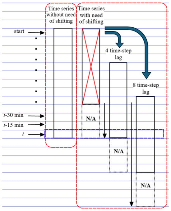
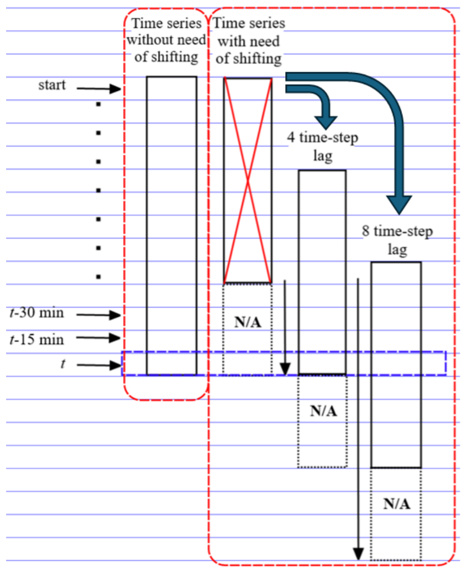
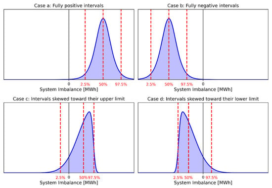
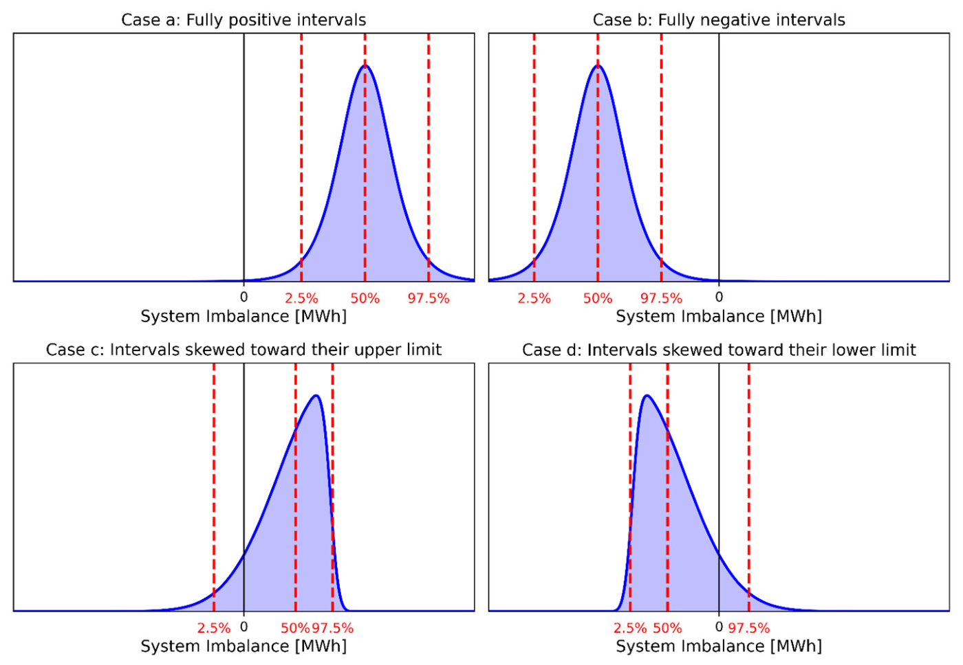


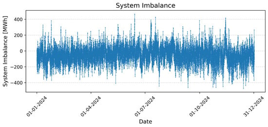
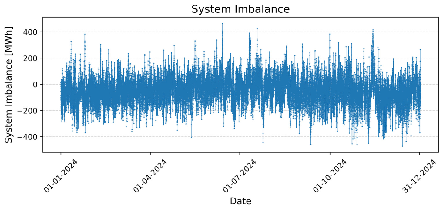
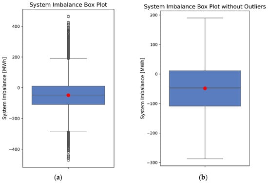
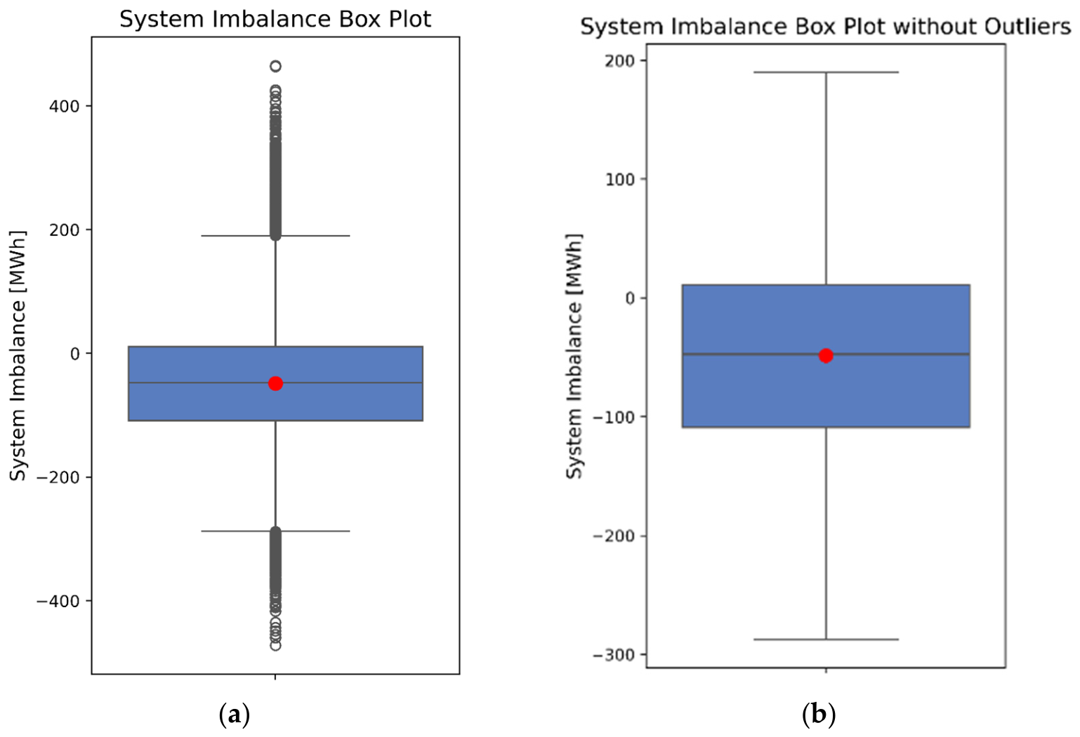
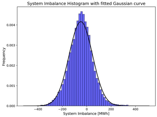
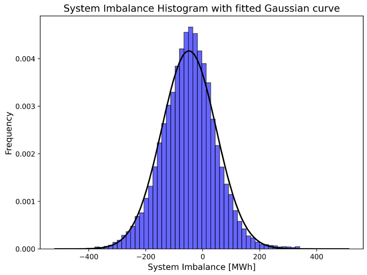
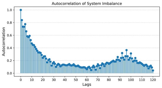
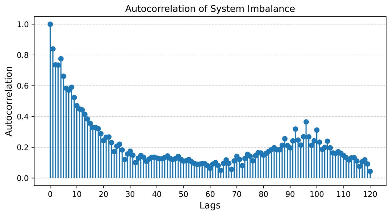
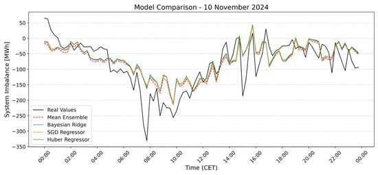
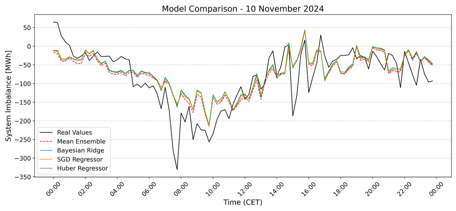
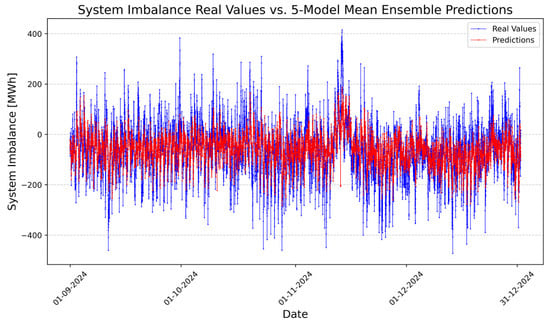
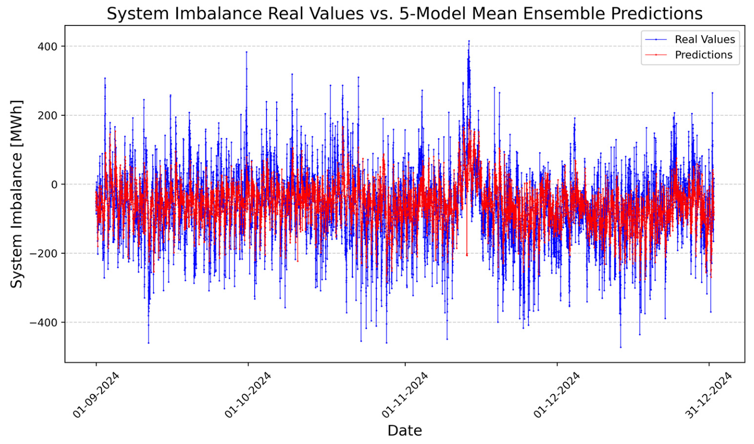
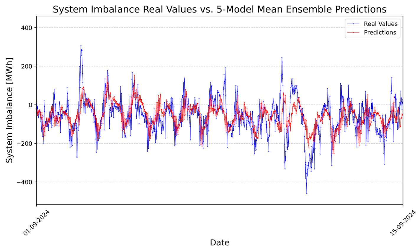
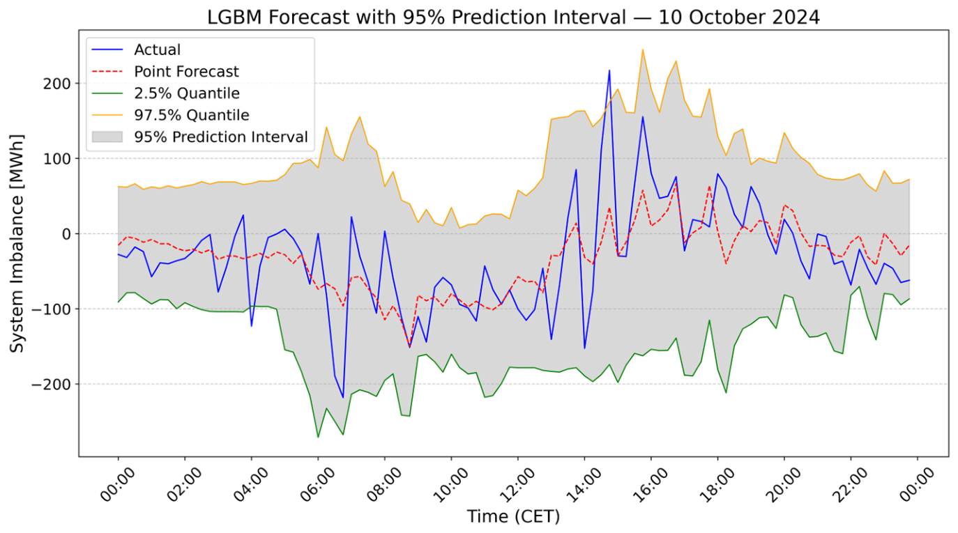

Disclaimer/Publisher’s Note: The statements, opinions and data contained in all publications are solely those of the individual author(s) and contributor(s) and not of MDPI and/or the editor(s). MDPI and/or the editor(s) disclaim responsibility for any injury to people or property resulting from any ideas, methods, instructions or products referred to in the content. |
© 2026 by the authors. Licensee MDPI, Basel, Switzerland. This article is an open access article distributed under the terms and conditions of the Creative Commons Attribution (CC BY) license.