


Abstract
Accurate photovoltaic (PV) forecasting depends on both model structure and the meteorological information available at different forecast horizons. This study evaluates hourly generation from a 7.5 kWp rooftop PV system at Brunel University of London using local sensor, weather station, and NASA POWER data. Long Short-Term Memory (LSTM), Random Forest (RF), and Gradient Boosting (GB) models were compared across seven input configurations and 0, 1, 3, 6, and 24 h horizons, with robustness assessed over five random seeds. For positive forecast horizons, the models used only meteorological observations available at or before the forecast issue time; no future weather forecasts corresponding to the target hour were supplied. Local sensor measurements provided the strongest same-hour estimation, whereas hybrid multi-source inputs were generally more effective for future forecasting. Under the native model formulations, LSTM achieved the lowest mean Root Mean Square Error at 1 and 3 h, while RF performed best at 6 and 24 h. An information-equivalent sensitivity analysis supplied tree-based models with the same 24 h predictor history as LSTM. History-aware boosting then matched the 1 h LSTM performance and substantially narrowed the difference at 3 h, indicating that part of the apparent short-horizon LSTM advantage was associated with access to recent temporal information rather than model architecture alone. Overall, the results demonstrate that meteorological data sources, forecast horizons, model family, and historical information representation should be considered jointly when designing short-term PV forecasting systems.
1. Introduction
The transition towards Net Zero has accelerated the deployment of renewable energy sources (RESs). Countries globally are progressively adopting RESs due to their high potential to decrease greenhouse gas emissions and reduce dependence on coal and gas. However, despite these environmental and economic benefits, renewable energy presents substantial challenges to power systems’ flexibility [1] and security [2]. Unlike traditional power generation, which operates in a predictable and controllable manner, RES output is directly influenced by meteorological and environmental conditions [3]. This inherent uncertainty compels industry stakeholders and researchers to investigate the correlations between RES output and weather patterns. Consequently, advanced short-term forecasting methodologies and sophisticated analytical techniques have become fundamental for improving RES integration, operating the forecast with the horizon spanning from minutes to hours based on time series datasets.
Among different types of RESs, photovoltaic (PV) power generation has demonstrated impressive growth. In 2022, global PV power generation increased by a record 270 TWh, up 26%, reaching almost 1300 TWh [4]. It displayed the largest power generation growth among all renewable technologies, surpassing wind for the first time in the history of RES development. This rapid expansion confirms the necessity of accurate short-term forecasting techniques to enhance grid integration and stability of operation.
As one of the world leaders in achieving Net Zero, the United Kingdom (UK), according to the Future Energy Scenarios 2024 [5], plans to significantly increase the amount of PV capacity from the current 15 GW to 40 GW by 2030 and exceeding 100 GW by 2050 under the Holistic Transition pathway. As PV becomes one of the key players in the UK energy market, accurate short-term forecasting of its generation requires advancements in PV forecasting technologies to support the integration of large-scale solar power and distributed generation.
A key issue in PV forecasting is the choice and quality of the meteorological data used as model inputs. Ground-based sensors provide specific site observations of irradiance and other environmental conditions, but reliable measurements depend on appropriate sensor calibration, maintenance, data acquisition and procedures of quality control [6,7]. Modelled and remotely sensed products provide an alternative source of meteorological and irradiance information, particularly where dedicated measurements are unavailable, although their accuracy can vary with location, climate, product formulation, spatial resolution and temporal aggregation [8,9,10]. Weather observations obtained from neighbouring stations can also provide useful spatial information, but their contribution to short-term solar forecasting depends on both their spatial relationship to the target site and the forecast lead time [11]. Satellite irradiance products provide broad spatial coverage, while ground measurements retain the advantage of direct site observations. Consequently, neither source should be assumed to be universally superior [8,9,10]. Studies combining ground observations with satellite and numerical data for weather prediction have shown that these sources can provide complementary information and improve intra-day solar forecasts [12,13].
The forecast horizon introduces an additional consideration because the information available to a forecasting model does not retain the same predictive value as the lead time increases. Reviews of solar forecasting methods distinguish between very short-term, intra-day and day-ahead forecasting and show that the suitability of ground observations, satellite information, data-driven methods and numerical weather prediction varies across these horizons [14,15]. Experimental studies support this distinction. Ground-based persistence and local observations can be particularly effective at very short horizons, satellite information can provide considerable value over the following few hours, while numerical weather prediction becomes increasingly relevant at longer lead times [13,16]. The performance ranking of forecasting methods is therefore difficult to generalise across studies because it also depends on the dataset, temporal resolution, forecast horizon and evaluation procedure [17]. This motivates evaluating alternative meteorological inputs over several lead times under the same experimental conditions.
A second consideration is the choice of forecasting algorithm. Long Short-Term Memory (LSTM) networks are well suited to sequential data because they can represent temporal dependencies, but greater architectural complexity does not imply that they will outperform conventional machine learning (ML) methods for every dataset or forecast horizon [18,19,20]. Tree-based ensemble models provide an important comparison because Random Forest (RF) and boosting algorithms can represent nonlinear relationships between meteorological predictors and PV generation and have shown competitive performance in PV forecasting applications [21,22,23]. Previous comparative studies have shown that PV forecasting performance depends on both model architecture and the information supplied to the model. Carrera and Kim [23] compared multiple ML methods under alternative meteorological input settings and reported substantial differences across both algorithms and weather information configurations. Dimitropoulos et al. [24] similarly compared ML and deep learning approaches under different data input cases and examined their performance across increasing forecast horizons. Alternative architectures have also been investigated: Zhou et al. [25] combined LSTM with an attention mechanism and compared it with persistence, AutoRegressive Integrated Moving Average with eXogenous inputs, multilayer perceptron and conventional LSTM approaches, while Olcay et al. [26] directly compared LSTM and RF for solar energy forecasting. Collectively, these studies indicate that model rankings are influenced by the forecasting horizon, input representation and experimental design. The comparison performed in this study therefore considers LSTM alongside RF and Gradient Boosting (GB) rather than assuming a priori that one model family is superior.
Accordingly, this paper investigates how the source of meteorological information influences PV generation forecasting accuracy across multiple forecast horizons. Hourly generation data from a rooftop PV installation at Brunel University of London are combined with three categories of meteorological information: local sensor measurements, weather station observations and satellite variables. Single-source and hybrid feature groups are evaluated using LSTM, RF and GB models at 0 h, 1 h, 3 h, 6 h and 24 h horizons. The 0 h experiment is treated as a same-hour estimation and data consistency test, while the positive lead times represent forecasting tasks.
The main objective of this work then is to determine how the usefulness of sensor, weather station, satellite and hybrid input data changes with the forecasting horizon and model family. The specific aims are formulated as follows:
- Develop a harmonised multi-source dataset for PV forecasting using local generation, sensor, weather station, and satellite variables.
- Compare the forecasting performance of single-source and hybrid meteorological feature groups under the same modelling framework.
- Evaluate whether particular models provide consistent advantages over other ones across different forecast horizons.
- Assess how the relative importance of data source quality, temporal information, and model structure changes between same-hour estimation and future PV generation forecasting.
- Assess whether observed differences between forecasting model families persist when equivalent 24 h historical information is provided to recurrent and tree-based models, and quantify their forecasting skill relative to persistence benchmarks.
The remainder of this paper is structured as follows: Section 2 provides a detailed description of the weather datasets utilised in the research, preprocessing techniques, forecasting models applied and assessment metrics. Section 3 presents the performance results of the forecasting models, comparing their accuracy based on different data sources, analysing the impact of various techniques and data sources on model performance, while also addressing potential limitations and future improvements. Finally, Section 4 summarises the key findings of the study, emphasising the importance of data selection and advanced forecasting techniques in improving the reliability of PV power generation predictions.
2. Materials and Methods
2.1. The Framework Proposed
In this section, Figure 1 illustrates the overall methodological framework, revealing the conducted research, structured through a multistage process. Each depicted stage encompasses distinct analytical procedures, serving as the basis for detailed elaboration provided in the subsequent sections of this paper.
Figure 1.
The framework of the research paper.
2.2. PV Installation Characteristics
This paper utilises the generation data of an experimental PV installation located on top of the Joseph Lowe building at Brunel University of London (Brunel University), previously titled Brunel University London, located within geographical coordinates 51.5308° N, 0.4740° W. This PV system integrates 22 solar panels with a total nominal capacity of 7.5 kilowatts peak. The installation is positioned on a flat rooftop, covering an approximate area of 300 m2 (15 × 20 m). All the panels are positioned to the south for the best performance, with the incline equal to 40°. The system’s design and configuration enable continuous monitoring of power output for investigating PV installation forecasting methodologies [27]. The PV installation is connected to a campus power distribution system, and the electric energy generated serves to satisfy the university’s needs. This also allows treating an existing PV as a negative demand for Brunel University.
For data access, the study utilises the physical device SMA Data Manager M [28], installed close to the PV installation for accurate real-time monitoring. The data exchange within the installation is facilitated by the Modbus standard messaging protocol, designed for reliable communication between devices. Modbus is a widely used communication protocol designed for industrial applications, enabling efficient data exchange between devices due to a simple message structure, embedded error-checking mechanisms, and defined master–slave interactions [29]. Additionally, the system uses Sunny Portal, powered by ennexOS [30], a cloud-based platform for monitoring and analysing PV system performance. The PV installation is connected to the campus power grid and serves two main objectives: to partially satisfy the campus electricity demand and act as an experimental platform for research conducted by the university’s departments and research centres.
A photographic image of the PV installation, its corresponding configuration diagram and Open Street Maps [31] with the exact coordinates are provided in Figure 2a, b, c and d, respectively.
Figure 2.
(a) Left camera photographic image of the PV installation located at Brunel. (b) Right camera photographic image of the PV installation located at Brunel. (c) Configuration diagram of the PV installation located at Brunel. (d) Spatial location of the PV installation.
The power generation data are historically available and recorded at 5 min intervals in watts (W), representing instant output at given intervals and allowing detailed exploration of the PV installation’s performance dynamics. To ensure consistency with the hourly meteorological datasets, the 5 min PV power observations were aggregated to hourly resolution. Since twelve instantaneous power measurements were available within each complete hour, hourly PV energy was calculated by discrete temporal integration using a fixed sampling interval of min, using the following mathematical formula:
where is the PV energy generated during hour h, expressed in watt-hours (Wh); is the j-th instantaneous PV power measurement within that hour, expressed in watts (W); and Δt = 5 min is the fixed interval between successive measurements. For a complete hour, twelve measurements are therefore incorporated into the hourly energy estimate. The resulting hourly PV energy series was used as the prediction target throughout the forecasting experiments.
The performance of Brunel’s PV installation is illustrated comprehensively in Figure 3a–d, which represent monthly, daily, hourly, high and low output. The power generation data available span from March 2023 to June 2024. To reduce the scale size, the units for the plots are transformed from Wh to kWh. The initial analysis indicates robust repetitive patterns: seasonal, monthly, and daily PV installation generation, demonstrating strong, consistent and predictable generation characteristics. The presence of these clear repetitive patterns confirms that an in-depth analysis of the PV installation generation is feasible and forecasting models can be effectively developed, potentially achieving a high level of accuracy. At the same time, the influence of weather variability and associated uncertainty is evident across the descriptive profiles shown in Figure 3, which were calculated from the quality-controlled PV generation series after the data cleaning procedures.
Figure 3.
(a) Monthly performance of Brunel’s PV installation March 2023–June 2024. (b) Daily performance of Brunel’s PV installation March 2023–June 2024. (c) The representation of the monthly generation (May 2024) of the PV installation. (d) Two days representing high and low output of PV installation (20 and 21 May 2024); all profiles are derived from the quality-controlled PV generation series used for subsequent model development.
2.3. Weather Conditions Datasets
Each forecasting model, regardless of its type, fundamentally relies on the dataset it is trained on, with the quality and characteristics of the data directly influencing its performance. In the context of RES power output forecasting, the accuracy of predictions is closely linked to the quality of the weather data used. To investigate and confirm this relationship, this paper utilises three reliable datasets, each differing significantly in terms of data source. Subsequently, in this sub-chapter, we provide a detailed overview of each dataset.
Sensor-based weather data—collected from the 3S-IS irradiance sensor [32], which is installed close to the PV installation. This sensor provides the following meteorological parameters: solar irradiance mean (W/m2) and ambient temperature of the PV installation (°C). The 3S-IS photovoltaic reference cell sensor records local solar irradiance on the sensor plane, therefore interpreted as local plane-of-array (POA) irradiance, south-facing, approximately 40° tilt.
Meteorological station data—the dataset was obtained through the Weather Query Builder of the Visual Crossing platform [33]. The platform’s Weather Data Application Programming Interface (API) provides access to a full block of historical weather information, data and indexes [34]. In the case of these data, solar radiation represents instant power at the moment of observation, while solar energy indicates the total accumulated solar energy over an hour or day. However, the Visual Crossing platform has limitations as the datasets are available only at daily and hourly time resolutions. The dataset for this research paper originates from the Hillingdon Borough weather data station, located in London, UK, at an estimated distance of 2 km from the PV installation at Brunel University.
Satellite-derived data—this dataset is obtained from the National Aeronautics and Space Administration (NASA) Prediction of Worldwide Energy Resources (POWER) project, which provides global meteorological data specifically tailored for renewable energy applications, as documented in NASA POWER [35]. The NASA POWER renewable energy development package combines satellite solar radiation products with meteorological fields derived from NASA data assimilation and modelling systems. However, the temporal resolution of available data is limited to hourly intervals, restricting detailed assessments that require higher-resolution inputs. For consistency with other datasets, this study utilises weather data with the exact coordinates of the PV installation at Brunel University (51.5308° N, 0.4740° W). The dataset includes a comprehensive range of meteorological factors from the RES sources development package [36].
Overall, the weather dataset available for the paper looks as shown in Table 1, with the abbreviation set added to represent all the weather features and to make working with them easier.
Table 1.
The weather dataset used for research investigations.
2.4. Dataset Formation and Data Processing
To configure the final dataset employed in this research, we integrated generation data from the PV installation with the meteorological parameters presented in Table 1. Additionally, numerical counters representing the year, month, day, and hour were subsequently included to achieve temporal consistency. The finalised dataset consists of continuous time series data spanning from 1 March 2023 to 30 June 2024, covering a period of 16 months and resulting in a structured array dimensioned approximately 11,700 × 50 cells. Since all the datasets described in the previous subsection contain primarily quantitative meteorological variables without explicitly defined qualitative attributes, the data were formatted in a float32 numeric representation.
Data quality control for the dataset included checks for missing values, duplicate timestamps, physically unrealistic measurements, and discontinuities [7]. The physical plausibility screening applied explicit variable-specific criteria. Local sensor temperature values (SEN_temp) below −40 °C or above 60 °C were treated as missing, while weather station precipitation values (WS_precip) below 0 mm or above 100 mm were rejected. Negative values in satellite UV-related variables were also treated as invalid, and positive or negative infinite values in numerical variables were converted to missing values. Six timestamp errors occurring at month boundaries were corrected. The expected UK daylight-saving-time transitions were retained, including the missing hour on 26 March 2023 and 31 March 2024, and the duplicated hour on 29 October 2023. British Summer Time (BST) denotes the UK summer-time period. Invalid observations including anomalous local sensor temperatures, extreme precipitation values, and satellite error codes (e.g., −999) were treated as missing and subsequently handled using the corresponding preprocessing procedure. Following outlier removal, missing numerical observations were reconstructed using temporal interpolation. Where required at the boundaries of a continuous series, forward or backward filling was applied to preserve the hourly sequence used for model construction. Where interpolation between the immediately preceding and following observations was appropriate, the corrected value was calculated as
where is the corrected observation at time t. This procedure preserved the continuous hourly sequence required for constructing LSTM input windows [37].
Daylight and nighttime periods were treated separately. For reproducibility, a binary daylight flag Dt was defined from solar geometry and irradiance observations as follows:
where denotes the daylight flag at hour t, is the satellite solar zenith angle, is the local sensor mean irradiance, is the weather station solar radiation, and is the satellite global horizontal irradiance. The logical means that satisfaction of any one criterion is sufficient for the hour to be classified as daylight. Measured PV generation itself was not used in the daylight classification, avoiding target-dependent classification.
Nighttime observations were retained within the chronological sequence but were not considered informative forecasting targets because PV generation is physically zero in the absence of solar irradiance. Therefore, model performance was evaluated primarily for daylight target hours, while complete daily profiles were reconstructed as
where D denotes daylight hours, is the model input vector and represents the forecasting model. This prevents deterministic nighttime zero values from artificially reducing forecasting errors.
The processed data were divided chronologically into training, validation and test sets [37,38]. Data before 1 January 2024 were used for training, 1 January–31 March 2024 for validation, and 1 April–30 June 2024 for independent testing. After quality control, the chronological partitions contained 7344 hourly observations in the training period, 2183 in the validation period, and 2184 in the independent test period. Following application of the daylight target definition described above, 4306 training, 947 validation, and 1521 test observations were classified as daylight target hours. Random temporal shuffling was not applied. For the LSTM models, input variables were standardised [39] using statistics calculated exclusively from the training set
where and are the training set mean and standard deviation of variable i. The same parameters were subsequently applied to the validation and test data. RF and GB models used the processed variables without standardisation. The same chronological partitions and quality-controlled dataset were used for all sensor, weather station, satellite and hybrid experiments.
2.5. Forecasting Models
Three forecasting algorithms were evaluated under a common experimental framework: LSTM, RF, and GB. LSTM represents a sequence learning architecture that processes temporal windows, whereas RF and GB provide tree-based benchmarks for nonlinear relationships between PV generation and meteorological predictors. The purpose of using these three model families was not to identify a universally superior algorithm, but to distinguish the effect of the model structure from the effects of the meteorological data source and forecast horizon. The primary experiment retained the native input representation of each model family: LSTM processed a 24 h sequential window, whereas RF and GB used predictors available at the forecast issue time. For all positive forecast horizons (h = 1, 3, 6, and 24), the predictor information was restricted to meteorological and PV observations available at or before the forecast issue time. No future meteorological forecasts describing conditions at the target time t + h were supplied to the models; the positive horizon experiments therefore represent observation-driven forecasting based on currently and historically available information. Because this difference in input representation could itself influence the relative performance of the model families, an additional information-equivalent sensitivity experiment was subsequently performed in which tree-based models were supplied with the same 24 h historical information window as the LSTM.
The LSTM models were implemented in PyTorch, version 2.13 [40], while RF and GB were implemented using the scikit-learn, version 1.9.0 [39] RandomForestRegressor and GradientBoostingRegressor classes, respectively. The principal model hyperparameters were fixed across data source configurations and forecast horizons. Only the input feature composition, forecast horizon, and random seed were varied. This controlled design was adopted so that differences in forecasting accuracy could be attributed primarily to the experimental factors investigated in this study rather than to configuration-specific hyperparameter tuning.
A personal computer with the following characteristics, Central Processing Unit (CPU) i7 11800H, Installed Physical Memory 32 GB, Graphical Processing Unit NVIDIA GeForce RTX 3060 6 GB, was used for conducting the experiment.
2.5.1. LSTM
LSTM is a recurrent neural network architecture designed to represent temporal dependencies through a gated memory mechanism [41]. In contrast to a conventional recurrent neural network, the LSTM cell regulates the retention, update, and transmission of information using forget, input, and output gates [42]. At time step t, the three gates are calculated as follows [41,42,43]
where the three gate outputs correspond to the forget, input, and output gates, respectively; the subscript t denotes the current time step, x is the input vector, h is the hidden state, W and U are trainable input and recurrent weight matrices, b represents the bias vectors, and σ(.) is the logistic sigmoid function. The candidate cell state, cell state, and hidden state are then determined by
where c represents the cell state, the tilde term represents the candidate cell state, tanh(.) is the hyperbolic tangent activation, and ⊙ denotes the Hadamard (element-wise) product. These operations enable the network to retain relevant historical information while suppressing information that is no longer useful for the forecasting task.
A graphical representation of the LSTM cell is depicted [44] in Figure 4.
Figure 4.
The structure of the LSTM cell.
In this study, each LSTM model used a fixed 24 h look-back window. For a forecast issued at time t, the preceding 24 hourly observations were used to estimate PV generation at time t+h, where h represents the forecast horizon
The implemented network contains one LSTM layer with 64 hidden units. The final hidden representation was passed through a dropout layer with a dropout probability [45] of 0.20, followed by a fully connected layer with 32 neurons and rectified linear unit (ReLU) activation, and a final linear output neuron. Model training used the Adam optimiser [46] with a learning rate of 0.001, a batch size of 64, and a maximum of 30 epochs. Early stopping was applied using validation loss [47] with a patience of six epochs, and the parameter state producing the minimum validation loss was restored for final prediction. To limit unstable parameter updates, the gradient norm was clipped at 1.0 [48].
The LSTM loss function was the Huber loss with delta = 0.05. The target PV generation was divided by the maximum PV generation observed in the daylight training subset before optimisation and converted back to the original scale after prediction. Huber loss was selected because it combines quadratic behaviour for small errors with linear behaviour for larger errors [49]. Here, e denotes the forecasting error and δ = 0.05
Numerical LSTM inputs were standardised using a StandardScaler fitted only to the daylight training windows. The same scaling parameters were subsequently applied to the validation and test sequences. Training and validation loss were calculated only for daylight target hours, although the complete chronological sequence, including nighttime observations, was retained inside the 24 h input windows. Nighttime PV predictions were reconstructed deterministically as zero, as described in Section 2.4.
2.5.2. RF
RF is an ensemble regression method that combines multiple decision trees [50]. Each tree is trained using a bootstrap sample of the training observations, while only a randomly selected subset of predictors is considered at each split. This decorrelates the individual trees and reduces the variance associated with a single regression tree while retaining the ability to represent nonlinear interactions between PV generation and meteorological variables.
For a forecast horizon h, the RF estimate is obtained by averaging the outputs of B regression trees [50]
where each T(.) represents an individual regression tree, B is the number of trees, and x is the feature vector available at the forecast issue time [50]. In the implemented model, B = 300 trees, max_features = “sqrt”, and min_samples_leaf = 2. The remaining RandomForestRegressor settings were retained at their scikit-learn defaults [39]. In particular, tree depth was not explicitly restricted. The random_state parameter was set separately for each robustness run, and n_jobs = −1 was used to allow parallel fitting across available CPU cores.
RF was trained on the processed variables in their original numerical scale because decision tree split locations depend on ordered thresholds rather than Euclidean distances or gradient-based parameter updates. Separate RF models were fitted for every input configuration and every forecast horizon. Unlike the LSTM, RF does not maintain an internal sequential hidden state; its temporal information is therefore supplied explicitly through the autoregressive (AR) PV variable and cyclic time descriptors included in the feature vector [17,22].
2.5.3. GB
GB is also based on regression trees, but the ensemble is constructed sequentially rather than independently [51]. At boosting iteration m, a new tree is fitted to reduce the residual error of the current ensemble, and its contribution is controlled by the learning rate η. The model update can be expressed as [51]
where F represents the current ensemble prediction, and T is the regression tree added at boosting iteration m. After M boosting iterations, the final PV forecast is represented by
where is the initial estimate, M is the number of boosting estimators, and η is the learning rate. The implemented GradientBoostingRegressor [39] used M = 250 estimators, η = 0.05, max_depth = 3, and min_samples_leaf = 2. The random_state parameter was changed according to the robustness seed. The relatively shallow trees restrict the complexity of each weak learner, while sequential boosting progressively models nonlinear relationships that remain unexplained by the preceding ensemble.
As for RF, GB used the processed input variables without standardisation. A separate GB model was fitted for each meteorological input configuration and forecast horizon. The GB model therefore provides a complementary tree-based benchmark: RF reduces variance by averaging many partially decorrelated trees, whereas GB reduces residual error by adding trees sequentially [22].
2.5.4. Common Model Comparison Framework
The model hyperparameters described above were fixed throughout the main robustness experiment. The experimental variables were the model family, meteorological input configuration, forecast horizon, and random seed. This distinction is important because the central objective of the paper is to determine how the predictive value of meteorological data changes with the lead time and model family, rather than to optimise a different architecture independently for each case. The fixed architecture and principal hyperparameters applied to the three forecasting models are summarised in Table 2.
Table 2.
Fixed characteristics of the forecasting models used in the experiment.
Table 2 describes the primary model family experiment. A supplementary information-equivalent sensitivity experiment was additionally supplied and is described in Section 2.5.5.
The AR generation predictor GEN_AR was constructed dynamically to prevent leakage in the same-hour experiment. At h = 0, the previous-hour PV value was used; for the future horizons, the PV value available at the forecast issue time was used:
The three model families do not receive inputs in exactly the same tensor form. For LSTM, each sample consists of 24 consecutive hourly observations, whereas RF and GB use the feature vector at the forecast issue time. If F denotes the number of predictors in a given feature configuration and N is the number of samples, the corresponding input dimensions are
This difference corresponds to the native input formulation adopted in the primary comparison. It should therefore not be interpreted as a fully information-equivalent test of model architecture. The additional analysis in Section 2.5.5 explicitly controls for this distinction by supplying the tree-based models with the same 24 h predictor history. Five forecast horizons were analysed, with h = 0 interpreted as same-hour estimation and consistency testing, and h = 1, 3, 6, and 24 representing genuine future forecasting tasks:
Seven input configurations were evaluated. The baseline consisted of GEN_AR together with six cyclic temporal descriptors: hour_sin, hour_cos, doy_sin, doy_cos, month_sin, and month_cos. The remaining configurations progressively added local sensor, Visual Crossing weather station, and NASA POWER satellite-derived information. The exact group definitions are summarised in Table 3.
Table 3.
Meteorological input configurations used for all three model families.
Robustness was assessed by repeating the complete model comparison using five random seeds [52]:
For LSTM, the seed controls neural network initialisation and stochastic mini-batch training. For RF and GB, the same seed was passed through the random_state parameter. The complete robustness design can therefore be represented as the Cartesian product of the three model families M, seven feature groups G, five forecast horizons H, and five random seeds S:
The complete design therefore comprises 525 model fits. For every fit, the chronological data partitions defined in Section 2.4 were preserved: observations before 1 January 2024 formed the training set, 1 January–31 March 2024 formed the validation set, and observations from 1 April 2024 onward formed the independent test set. Random temporal shuffling between these periods was not applied. Model performance was assessed primarily for daylight target observations using the metrics defined in Section 2.6.
2.5.5. Information-Equivalent Model Sensitivity Analysis
To avoid confusion with the GB model used in the primary experiment, the history-aware histogram-based implementation is hereafter denoted HistGB. The primary model family comparison used the native input representation of each forecasting algorithm. Consequently, the LSTM received a 24 h sequence of predictor observations, whereas RF and GB received a single predictor vector corresponding to the forecast issue time. To determine whether the observed model family ranking was influenced by this difference in historical information availability, an additional sensitivity experiment was performed in which the tree-based models were supplied with the same 24 h information window used by the LSTM.
For each prediction issued at time, the preceding 24 hourly feature vectors were flattened into a single tabular vector
where denotes the complete predictor vector available at the forecast issue time. Therefore, if a configuration contained F predictors, the history-aware tree model received 24F input variables. The same chronological training, validation and test periods, daylight target definition, forecast horizons and five random seeds used in the primary experiment were retained.
The sensitivity analysis focused on the hybrid raw and hybrid BST configurations because these represented the most comprehensive multi-source information sets and were consistently among the strongest configurations in the primary experiment. RF retained the same principal settings as in the main experiment, including 300 trees, max_features = , and min_samples_leaf = 2.
A HistGB model was additionally evaluated as a history-aware boosting sensitivity model. This model is reported separately from the GradientBoostingRegressor used in the primary experiment and is not intended to replace the original GB benchmark. Its purpose is to test whether a boosting architecture supplied with the same 24 h information window can reproduce the apparent short-horizon advantage observed for the LSTM. HistGB settings include 250 maximum iterations, learning rate 0.05, max depth 3, minimum samples per leaf 2, L2 = 0, early stopping with 10% internal validation and patience 20.
2.6. Model Assessment Metrics
Forecast accuracy was assessed using four metrics employed consistently throughout the experiment: Mean Absolute Error (MAE) [53], Root Mean Square Error (RMSE) [24,54], normalised Root Mean Square Error (nRMSE) [55], and the coefficient of determination (R2) [54]. The primary evaluation was performed on the 1521 daylight target observations in the independent test period (1 April–30 June 2024), because nighttime PV generation was reconstructed deterministically as zero. Full day results were retained as a secondary diagnostic, but model ranking and the main comparisons reported in the Results section were based on daylight-only performance [37].
MAE measures the average magnitude of the forecasting error without weighting large deviations disproportionately. For N evaluated daylight observations, MAE is defined as
where and denote the measured and forecast hourly PV generation, respectively. MAE is expressed in the same units as the target variable (Wh in this study), and lower values indicate better predictive accuracy.
RMSE applies a quadratic penalty to the individual errors and is therefore more sensitive than MAE to relatively large forecasting deviations. It was used as the principal model ranking criterion:
Because MAE and RMSE retain the physical scale of PV generation, nRMSE was additionally used to express forecasting error relative to the maximum observed hourly PV generation in the quality-controlled dataset. The implementation used the same observed peak value for all model families, input configurations, horizons, and random seeds:
The nRMSE is dimensionless and reported as a percentage of the observed PV peak, which allows forecasting errors to be interpreted relative to the scale of the installation. Lower nRMSE values indicate higher forecasting accuracy.
The coefficient of determination, R2, was used to quantify model performance relative to a constant predictor equal to the mean measured PV generation of the evaluated subset. It is calculated as
where is the mean measured PV generation over the evaluated observations. Values of R2 closer to 1 indicate stronger agreement between forecasts and observations, whereas R2 ≤ 0 indicates that the model does not outperform the corresponding mean value reference for that evaluation subset.
Robustness was assessed over the five random seeds [52] S = {1, 7, 21, 42, 100}. For every fixed combination of model family, meteorological input configuration, and forecast horizon, each performance metric q was therefore summarised by its mean and sample standard deviation across K = 5 runs:
The Results section therefore reports mean ± standard deviation across seeds rather than relying on a single stochastic run. Mean daylight test RMSE was used as the primary ranking criterion, while MAE, nRMSE, and R2 were used as complementary measures of absolute error, scale-normalised error, and goodness of fit, respectively.
2.6.1. Persistence Benchmarks and Forecast Skill
In addition to the AR temporal model configuration, three non-parametric persistence forecasts were evaluated to provide operationally interpretable reference benchmarks. Current value persistence assumes that the latest observed PV output remains unchanged over the forecast horizon:
Previous-day same-hour persistence uses the measured PV generation from the corresponding hour of the preceding day:
A solar geometry-adjusted persistence benchmark was additionally evaluated for short forecasting horizons to account for the deterministic change in solar position between the forecast issue time and the target hour using a mathematical expression:
where denotes the solar geometry-adjusted persistence forecast for target time t+h, P_t is the PV generation observed at forecast issue time t, and θ_t and θ_(t+h) are the solar zenith angles at the forecast issue and target times, respectively. The formulation preserves the persistence assumption for short-term atmospheric conditions while adjusting the expected PV output for the deterministic change in solar elevation. When cos(θ_t) <= 0, the persistence prediction was set to zero.
For each horizon, the persistence benchmark achieving the lowest daylight test RMSE was used as the strongest naive reference.
Forecast skill (FS) relative [55] to a benchmark was calculated as
where positive values indicate an improvement over the reference forecast and FS = 0 corresponds to equal performance.
2.6.2. Statistical Uncertainty of Forecast Comparisons
Random seed variability quantifies the stochastic variation associated with model fitting, but does not quantify uncertainty associated with the finite test period itself. Therefore, the principal history-aware model and persistence comparisons were additionally evaluated using paired block bootstrap resampling of the independent daylight test predictions.
Complete target days were used as resampling blocks in order to retain the dependence among hourly forecasting errors occurring within the same day. A total of 5000 bootstrap resamples were generated. For each resample, RMSE was recalculated for the compared forecasting methods and the paired difference in RMSE was obtained. The 2.5th and 97.5th percentiles of the resulting distribution were used to form a 95% confidence interval (CI). A model difference was treated as resolved at the 95% bootstrap level when the confidence interval for the paired RMSE difference did not include zero.
3. Results and Discussion
The forecasting results are examined from eight complementary perspectives: physical and temporal consistency of the integrated dataset, forecast horizon dependence, meteorological data source performance, comparison of the LSTM, RF and GB model families, robustness across repeated random seeds, information-equivalent model comparison, forecasting skill relative to persistence benchmarks, and sensitivity to satellite temporal alignment. Unless stated otherwise, the principal results refer to daylight observations in the independent test period from 1 April to 30 June 2024.
3.1. Dataset and Temporal Validation
The first analysis examined whether the merged PV and meteorological datasets retained the expected physical relationship between solar irradiance and measured PV generation. The local on-site irradiance signal showed a same-hour Pearson correlation of approximately r = 0.994 with PV generation. In comparison, the raw NASA POWER GHI series produced a lower same-hour correlation of approximately r = 0.862. A one-hour displacement diagnostic increased the satellite correlation to approximately r = 0.910, indicating that the satellite variables were more sensitive to temporal convention than the local sensor measurements [8,9,35]. This result supports the correctness of the local PV sensor merge while motivating a separate temporal alignment sensitivity analysis for the satellite data rather than treating the satellite timestamps as erroneous.
To quantify the contribution of the different data sources under controlled conditions, the same LSTM architecture and chronological data split were used while only the input feature set was changed. For each forecast horizon h, the prediction target was PV generation at time t+h:
Using a 24 h look-back window (L = 24), the AR time baseline contained lagged PV generation together with temporal descriptors, the sensor configuration added the local on-site measurements (SEN_irr_mean, and SEN_temp), and the hybrid raw configuration further combined the local sensor variables with the Visual Crossing weather station variables and NASA POWER satellite variables:
where denotes the temporal features, the local sensor measurements, the Visual Crossing variables, and the NASA POWER variables under their original temporal alignment. The term “raw” therefore refers to the original satellite timestamp convention, not to uncleaned data. For h = 0, the contemporaneous PV generation value was not supplied as an input; the AR PV component remained lagged, preventing direct target leakage. This design allows differences in accuracy to be attributed primarily to the additional meteorological information introduced by each feature configuration.
The h = 0 experiment was used as a same-hour consistency diagnostic rather than as a future forecast. Under the controlled LSTM source comparison, the sensor configuration achieved MAE = 62.779 Wh, RMSE = 263.085 Wh, nRMSE = 4.057%, and R2 = 0.977 on 1521 daylight test observations. The AR time baseline produced RMSE = 1163.425 Wh, nRMSE = 17.939%, and R2 = 0.547. Thus, incorporating the local sensor variables reduced the same-hour RMSE by 77.39% relative to the temporal baseline. The hybrid raw configuration was only slightly weaker than the sensor configuration at h = 0 (RMSE = 278.937 Wh; nRMSE = 4.301%; R2 = 0.974), confirming that the dominant same-hour information is contained in the local irradiance signal [17]. The measured and predicted daylight PV profiles obtained with the h = 0 sensor configuration are compared in Figure 5. Measured and predicted PV generation for the h = 0 sensor configuration during a representative subset of the daylight test period. Performance metrics reported in the text were calculated using all 1521 daylight test observations.
Figure 5.
Measured and predicted PV generation for the h = 0 sensor configuration on the daylight test set.
Figure 5 shows that the model reproduces both the timing and magnitude of the principal daytime generation peaks, while the largest residuals occur around rapidly changing intra-day conditions. Taken together, the correlation analysis and h = 0 forecasting performance provide an empirical check that the quality-controlled dataset is physically coherent and suitable for the subsequent multi-horizon experiments.
3.2. Forecast Horizon Dependence
Forecast accuracy worsened systematically as the prediction horizon increased. In the controlled LSTM comparison, the best daylight RMSE increased from 263.085 Wh at h = 0 to 540.625 Wh at h = 1, 728.492 Wh at h = 3, 956.735 Wh at h = 6, and 1046.899 Wh at h = 24. The corresponding nRMSE increased monotonically from 4.057% to 8.336%, 11.233%, 14.752%, and 16.142%, respectively. The h = 24 RMSE was therefore almost four times the h = 0 value, reflecting the progressive loss of information about future irradiance and cloud conditions as the forecast horizon expands [13,21]. The best-performing meteorological input configuration at each forecast horizon in the controlled LSTM experiment is summarised in Table 4.
Table 4.
Best meteorological input configuration at each forecast horizon in the controlled LSTM experiment.
For quantitative comparison with the AR time baseline, the relative RMSE improvement was calculated as
Using Equation (37), the best LSTM configuration reduced RMSE relative to the AR time baseline by 77.39% at h = 0, 53.07% at h = 1, 32.07% at h = 3, 13.94% at h = 6, and 10.34% at h = 24. The diminishing relative improvement is important: meteorological information remains beneficial at all horizons, but the deterministic relationship between currently observed conditions and future PV generation weakens as the prediction target moves further ahead. The horizon-dependent change in daylight nRMSE across the meteorological input configurations is illustrated in Figure 6.
Figure 6.
Daylight nRMSE across forecast horizons and meteorological input configurations in the controlled LSTM experiment.
The measured versus predicted profiles at h = 1 and h = 3 are shown in Figure 7 and Figure 8, respectively. The actual versus predicted profiles provide the same pattern visually. At h = 1, the hybrid raw model follows the major PV peaks closely but shows larger deviations during rapid ramps than the h = 0 sensor model. At h = 3, the timing of the broad daily profile remains well represented, while peak amplitude errors become more pronounced.
Figure 7.
Measured and predicted PV generation for the h = 1 hybrid raw configuration.
Figure 8.
Measured and predicted PV generation for the h = 3 hybrid raw configuration.
3.3. Meteorological Data Source Comparison
The preferred meteorological source depended strongly on the forecast horizon. The local sensor configuration was clearly superior for h = 0, where same-hour irradiance directly represents the physical forcing of the PV system [13,16]. Its nRMSE of 4.057% was substantially lower than weather station (10.445%), satellite raw (9.480%), and satellite BST-adjusted (9.190%). This result is consistent with the very high same-hour correlation between local irradiance and generation.
For future horizons, however, the ranking changed. At h = 1 and h = 3, the hybrid raw configuration produced the lowest errors, with RMSE values of 540.625 Wh and 728.492 Wh and R2 values of 0.902 and 0.822, respectively. At h = 3, satellite raw alone (RMSE = 795.689 Wh; nRMSE = 12.269%; R2 = 0.788) also outperformed both the sensor configuration (1008.768 Wh; 15.554%; R2 = 0.659) and the weather station configuration (888.339 Wh; 13.697%; R2 = 0.736). This indicates that the broader solar radiation descriptors available from NASA POWER add useful information once the target is displaced from the current observation time.
At h = 6, the differences between the strongest multi-source alternatives narrowed. Hybrid BST-adjusted achieved RMSE = 956.735 Wh, compared with 962.355 Wh for hybrid raw and 981.817 Wh for the weather station configuration. At h = 24, hybrid BST-adjusted again provided the lowest error (1046.899 Wh), although weather station (1052.174 Wh), satellite raw (1055.721 Wh), and sensor (1057.199 Wh) were very close. Consequently, the results do not support a universal ranking in which one meteorological source is optimal at every horizon. Instead, local measurements dominate same-hour estimation, whereas combining heterogeneous meteorological information is more robust for future forecasting. For completeness, the daylight nRMSE values obtained for all meteorological input configurations and forecast horizons are reported in Table 5.
Table 5.
Daylight nRMSE (%) by meteorological input configuration in the controlled LSTM experiment.
3.4. Model Family Comparison
The final robustness benchmark extended the analysis from data source selection to model family selection by evaluating LSTM, RF, and GB across five random seeds. The horizon-level winners demonstrate that no single algorithm dominated the complete forecasting problem [21]. RF produced the best mean performance at h = 0, h = 6, and h = 24, whereas LSTM produced the best mean performance at h = 1 and h = 3. The best five-seed model and input configuration identified at each forecast horizon are summarised in Table 6.
Table 6.
Best five-seed model family configuration at each forecast horizon.
At h = 0, RF combined with hybrid BST-adjusted inputs achieved RMSE = 253.36 Wh, nRMSE = 3.91%, and R2 = 0.978. For the short future horizons, LSTM with hybrid raw inputs was strongest: RMSE = 535.21 Wh and R2 = 0.904 at h = 1, and RMSE = 737.53 Wh and R2 = 0.818 at h = 3. RF regained the advantage at h = 6 using hybrid raw inputs (RMSE = 952.92 Wh; R2 = 0.696) and at h = 24 using hybrid BST-adjusted inputs (RMSE = 1038.81 Wh; R2 = 0.639). GB remained competitive, particularly at h = 1, but it did not produce the lowest five-seed mean RMSE at any of the five horizons. To provide a direct graphical comparison of the model families, Figure 9 presents the best-performing configuration within each family at every forecast horizon, using the five-seed mean daylight nRMSE and its variability across repeated runs.
Figure 9.
Comparison of the best-performing LSTM, RF, and GB configurations across forecast horizons. Points represent the mean daylight nRMSE over five random seeds, and error bars indicate ±1 standard deviation. For each model family and horizon, the plotted value corresponds to the input configuration with the lowest mean RMSE.
The primary model family comparison therefore indicates a horizon-dependent transition in forecasting performance. Under the native input representation of each algorithm, LSTM achieved the lowest mean RMSE at 1–3 h, while RF was more competitive at the same-hour, 6 h and 24 h horizons. The graphical comparison also shows that the differences between the three model families are relatively small at several horizons, particularly at 1, 3, and 24 h, despite changes in the identity of the best-performing family. However, because LSTM processes a complete 24 h input sequence while the primary RF and GB models use a single issue time feature vector, this result cannot by itself determine whether the short-horizon LSTM advantage arises from recurrent model structure or from access to a richer representation of recent temporal history. This distinction is examined directly through the information-equivalent sensitivity analysis presented in Section 3.6.
3.5. Robustness Across Random Seeds
The principal model rankings were tested using five random seeds: 1, 7, 21, 42, and 100. The results were not driven by a single favourable initialisation [52]. At h = 0, RF with hybrid BST-adjusted inputs was the best configuration in all five seed runs (5/5). At h = 6, RF with hybrid raw inputs also won 5/5 runs. At h = 24, RF with hybrid BST-adjusted inputs won 4/5 runs. The h = 1 case was more competitive: LSTM with hybrid raw inputs won 3/5 seed runs, while GB with hybrid raw inputs won the remaining 2/5. At h = 3, LSTM with hybrid raw inputs produced the best five-seed mean performance.
These seed-level results strengthen two conclusions. First, the RF advantage at h = 0 and h = 6 is highly stable rather than an artefact of stochastic training. Second, the h = 1 horizon represents a genuinely competitive region in which LSTM and GB can exchange the leading position between runs, even though LSTM remains best on the five-seed mean. For this reason, the manuscript reports horizon-level rankings using the repeated-seed mean metrics rather than the best individual run.
Repeated seed analysis therefore establishes the stability of the native input model rankings with respect to stochastic model fitting. It does not, however, address uncertainty arising from the finite test period or differences in the historical information supplied to the model families; these issues are examined separately in Section 3.6 and Section 3.7.
3.6. Information-Equivalent Model Comparison
To assess whether the model family ranking observed in the primary experiment was influenced by unequal access to recent historical information, RF and the HistGB sensitivity model were supplied with the same 24 h predictor window used by the LSTM. The analysis was performed for the four positive forecast horizons using the hybrid raw and hybrid BST configurations and five random seeds.
The information-equivalent comparison substantially narrowed the apparent advantage of LSTM at the shortest forecast horizons. At h = 1, history-aware HistGB with hybrid raw inputs achieved a mean RMSE of 534.57 ± 2.54 Wh, nRMSE of 8.24%, and R2 = 0.904. This result is practically identical to the mean RMSE of 535.21 Wh obtained by LSTM with hybrid raw inputs in the primary experiment. History-aware RF achieved a higher RMSE of 585.94 ± 1.11 Wh.
At h = 3, history-aware HistGB achieved 747.63 ± 2.39 Wh, compared with 782.12 ± 1.97 Wh for history-aware RF. The corresponding LSTM result from the primary experiment was 737.53 Wh. Thus, LSTM retained a small numerical advantage at 3 h, but the difference relative to history-aware boosting was substantially smaller than suggested by the native input comparison.
At h = 6, the strongest history-aware boosting and RF results were 953.69 ± 5.04 Wh and 966.85 ± 2.92 Wh, respectively. These values are close to the original RF hybrid raw result of 952.92 Wh, indicating that explicitly supplying 24 h of historical predictors did not materially improve the RF performance at this horizon.
At h = 24, history-aware RF with hybrid raw inputs achieved the lowest RMSE of 1024.56 ± 2.28 Wh, corresponding to nRMSE = 15.80% and R2 = 0.648. This improved on the primary RF result of 1038.81 Wh and retained the conclusion that RF is highly competitive at the longest horizon considered.
Overall, the information-equivalent experiment modifies the interpretation of the model family comparison. The 1 h LSTM advantage observed in the primary experiment largely disappears when a boosting model receives the same historical information window, while a small LSTM advantage remains at 3 h. Consequently, the short-horizon results should not be attributed solely to recurrent architecture; the representation and availability of recent temporal information also contribute materially to forecasting performance. The results are reflected in Table 7.
Table 7.
Information-equivalent 24 h history sensitivity results.
3.7. Persistence Benchmarks and Statistical Uncertainty
The forecasting models were additionally compared with non-parametric persistence benchmarks to determine whether the reductions in forecast error represented meaningful predictive skill rather than improvements only relative to the AR temporal ML baseline. The strongest naive reference varied with the forecast horizon. Solar geometry-adjusted persistence produced the lowest persistence RMSE at 1 h and 3 h, whereas previous-day same-hour persistence was strongest at 6 h. At 24 h, current value and previous-day same-hour persistence were equivalent for the evaluated formulation.
The best history-aware model achieved positive forecast skill relative to the strongest persistence benchmark at every future horizon. At 1 h, HistGB reduced RMSE from 674.08 Wh for solar geometry-adjusted persistence to 534.57 Wh, corresponding to a forecast skill of 20.7%. At 3 h, RMSE decreased from 1269.14 Wh to 747.63 Wh, giving a forecast skill of 41.1%. At 6 h, the best model reduced RMSE from 1367.18 Wh to 953.69 Wh, corresponding to a 30.2% forecast skill. At 24 h, history-aware RF reduced RMSE from 1367.18 Wh to 1024.56 Wh, equivalent to a 25.1% forecast skill.
Paired day block bootstrap analysis confirmed that these improvements were not explained by sampling variation within the independent test period. Relative to the strongest persistence benchmark, the mean paired RMSE differences were −139.75 Wh at 1 h (95% CI: −164.17 to −114.29 Wh), −522.25 Wh at 3 h (−594.66 to −447.23 Wh), −412.04 Wh at 6 h (−536.31 to −290.39 Wh), and −341.93 Wh at 24 h (−448.30 to −233.26 Wh). In all four cases, the CI remained entirely below zero.
The same analysis also clarifies the strength of the model family differences. HistGB produced significantly lower RMSE than history-aware RF at 1 h and 3 h, with paired differences of 51.39 Wh (95% CI: 33.21–69.40 Wh) and 34.96 Wh (7.85–61.67 Wh), respectively, expressed as RF minus HistGB. At 6 h, the 13.38 Wh difference was not statistically resolved because the 95% confidence interval ranged from −19.46 to 45.99 Wh. At 24 h, history-aware RF outperformed the strongest history-aware HistGB configuration by 28.92 Wh, with a 95% CI of 2.14–54.96 Wh. The results of the persistence benchmark are provided in Table 8.
Table 8.
FS relative to the strongest persistence benchmark.
FS relative to the strongest persistence benchmark by forecast horizon are reflected in Figure 10.
Figure 10.
Forecast skill of history-aware RF and HistGB relative to the strongest persistence benchmark at each forecast horizon.
3.8. Satellite Temporal Alignment Sensitivity
Satellite variables were evaluated in their original temporal configuration and in a BST-adjusted sensitivity configuration. The purpose of this analysis was not to correct an assumed timestamp error, but to quantify how sensitive the forecasting results are to alternative temporal harmonisation of remotely derived variables.
The percentage change in RMSE caused by the BST-adjusted representation was calculated as
The corresponding RMSE values and relative changes between the raw and BST-adjusted satellite configurations are summarised in Table 9.
Table 9.
RMSE sensitivity to raw and BST-adjusted satellite timing. Negative change denotes lower RMSE after BST adjustment.
The sensitivity analysis shows that the timing adjustment is not uniformly beneficial. For the satellite-only configuration, BST adjustment improved h = 0 RMSE by 3.06%, but worsened RMSE by 4.15% at h = 1 and 10.32% at h = 3; the changes at h = 6 and h = 24 were small (+1.21% and +0.29%). The hybrid configurations show the same short-horizon pattern: BST adjustment increased RMSE by 7.01% at h = 1 and 10.84% at h = 3. In contrast, it reduced RMSE slightly at h = 6 (−0.58%) and more clearly at h = 24 (−3.37%).
The information-equivalent sensitivity experiment produced the same general timing pattern. For history-aware RF, use of the BST-adjusted hybrid configuration increased RMSE relative to hybrid raw by 7.61%, 9.35%, and 1.93% at 1 h, 3 h, and 6 h, respectively, while the difference at 24 h was only 0.29%. History-aware HistGB showed corresponding changes of +7.43%, +11.58%, +4.02%, and −0.30%. These results reinforce the conclusion that the raw satellite representation is preferable at short intra-day horizons, whereas the timing convention has little practical influence by 24 h.
Accordingly, the raw satellite representation should remain the primary short-horizon configuration, particularly at 1–3 h, while the BST-adjusted representation is useful as a sensitivity case and becomes competitive at longer horizons. More importantly, the absence of a consistent improvement after temporal shifting indicates that the observed source differences cannot be reduced to a simple one-hour timestamp correction. They reflect a combination of source temporal conventions, spatial averaging, and the different information content of local, station, and satellite-derived variables.
The spatial generalisability of these findings should also be considered. The present analysis is based on a single rooftop PV installation in London, and the observed relationships between local sensor, weather station and satellite inputs are therefore conditional on the meteorological conditions and spatial characteristics of this site. Short-term irradiance variability can differ substantially between locations because of differences in cloud development and movement, local terrain, coastal exposure and other geographical effects. Consequently, the absolute forecasting errors and the ranking of meteorological input sources reported here should not be interpreted as universally transferable to other locations. Validation across multiple PV installations representing different climatic and geographical conditions would be required to determine the extent to which the observed source- and horizon-dependent relationships generalise beyond the present site.
From an operational perspective, these results do not identify a single forecasting algorithm that should be applied universally to all PV installations. For plants, connected to the grid, model selection should be aligned with the decision horizon: the short intra-day horizons examined here favour LSTM or history-aware boosting approaches, whereas RF becomes competitive at the longer horizons. The relatively small differences between model families at several horizons also suggest that computational complexity and data availability should be considered alongside forecasting accuracy when selecting a practical implementation. For a self-consumption installation, the underlying PV forecasting task remains similar, but the forecast would typically form part of a broader energy management problem that also includes electricity demand and, where applicable, battery operation. The preferred forecast horizon may therefore differ according to the operational decision being supported. Since demand forecasting, storage scheduling and energy management optimisation were not modelled in this study, the results should not be interpreted as identifying a universally optimal forecasting architecture for self-consumption applications.
Overall, the Results and Discussion identify a consistent but more nuanced horizon-dependent pattern. Local sensor measurements provide the strongest physical information for same-hour PV estimation, whereas hybrid meteorological inputs are generally most effective for future forecasting. Under the native input formulation, LSTM achieves the lowest mean RMSE at 1–3 h and RF is stronger at 6–24 h. However, when equivalent 24 h historical information is supplied to tree-based models, the apparent LSTM advantage at 1 h largely disappears and becomes relatively small at 3 h. This demonstrates that model performance depends not only on the forecasting architecture but also on how recent temporal information is represented. All of the strongest history-aware models also substantially outperform persistence benchmarks, with a forecast skill of approximately 21–41% across the evaluated horizons. The combined evidence therefore supports joint consideration of the data source, forecast horizon, model structure and historical information availability when designing short-term PV forecasting systems.
4. Conclusions and Future Work
This study compared the influence of the meteorological data source, forecast horizon, and model family on short-term PV generation forecasting using LSTM, RF, and GB models. The results show that no single input configuration or forecasting algorithm was consistently superior across all horizons. For same-hour estimation, the local sensor configuration provided the strongest LSTM performance, with RMSE = 263.085 Wh, nRMSE = 4.057%, and R2 = 0.977, reducing RMSE by 77.39% relative to the AR temporal baseline. For future forecasting, hybrid multi-source inputs were generally more effective. The best mean results were obtained by LSTM with hybrid raw inputs at 1 h and 3 h horizons, with RMSE values of 535.21 Wh and 737.53 Wh, respectively, whereas RF provided the strongest performance at 6 h and 24 h, with RMSE values of 952.92 Wh and 1038.81 Wh. These results indicate that the predictive value of meteorological information changes with the lead time and that model selection should therefore be horizon-specific rather than based on a single universally preferred forecasting method. However, the information-equivalent sensitivity analysis showed that part of the apparent short-horizon LSTM advantage was associated with access to the 24 h sequential information window. When the same historical information was provided to a boosting model, the 1 h RMSE decreased to 534.57 Wh, effectively matching the primary LSTM result of 535.21 Wh, while at 3 h, the corresponding difference was reduced to approximately 10 Wh. This indicates that model architecture and temporal information representation should not be interpreted independently.
The comparison also demonstrates that local measurements are particularly valuable for representing contemporaneous PV behaviour, while combining local sensor, weather station, and satellite information becomes more beneficial as the forecasting horizon increases. Forecast accuracy progressively decreased with lead time, with the best nRMSE increasing from 8.25% at 1 h to 16.02% at 24 h, while the corresponding R2 decreased from 0.904 to 0.639. The comparison with persistence further confirmed that the observed improvements represent genuine forecasting skill. Relative to the strongest naive benchmark at each horizon, the best history-aware models reduced RMSE by 20.7% at 1 h, 41.1% at 3 h, 30.2% at 6 h, and 25.1% at 24 h. Paired day block bootstrap analysis showed that all four improvements remained statistically significant at the 95% confidence level. Collectively, these findings show that forecast performance is jointly determined by meteorological information source, lead time, model architecture, and the historical information made available to the forecasting model.
Several limitations should be considered when interpreting the results. First, the analysis is based on a single 7.5 kWp PV installation and approximately 16 months of observations, and the quantitative model rankings may therefore vary across locations, climates and system configurations. Second, the positive horizon experiments use meteorological observations available up to the forecast issue time rather than operational weather forecasts describing future atmospheric conditions. The 24 h results should consequently be interpreted as data-driven forecasts conditional on historical meteorological information rather than as a complete operational day-ahead forecasting system. Third, the primary LSTM, RF and GB experiment uses the native input representation of each model family; the additional information-equivalent experiment was therefore introduced specifically to assess the sensitivity of model family conclusions to historical information availability.
Future work should extend the analysis to multiple PV installations and longer multi-year datasets to assess the generalisability of the observed relationships. Particular attention should also be given to operational forecasting at positive horizons by incorporating meteorological forecasts available at the forecast issue time, rather than relying solely on observed weather variables. Further work should additionally investigate the temporal characteristics of satellite data, including Coordinated Universal Time/local time harmonisation and explicit treatment of BST transitions, and apply feature ablation or interpretability methods to identify which meteorological variables provide the greatest additional predictive value within the hybrid configurations.
Author Contributions
Conceptualisation, methodology, software, validation, formal analysis, writing—original draft preparation, visualisation, D.H.; writing—review and editing, C.S.L.; supervision, project administration, G.T. All authors have read and agreed to the published version of the manuscript.
Funding
This research received no external funding.
Data Availability Statement
The photovoltaic generation and local sensor data supporting the findings of this study are available from the corresponding author upon request. NASA POWER meteorological data are publicly available from the NASA POWER project. Weather station data were obtained from Visual Crossing Weather under licence. Restrictions apply to the redistribution of the underlying Visual Crossing raw weather data. These data can be obtained directly from Visual Crossing subject to its applicable terms and licensing conditions.
Acknowledgments
The authors would like to thank the anonymous reviewers and the editor for their constructive comments and suggestions, which significantly improved the quality of this manuscript.
Conflicts of Interest
The authors declare no conflicts of interest.
Nomenclature, Abbreviations and Mathematical Representation
The following nomenclature and abbreviations are used in this manuscript:
| Abbreviation | Full term |
| API | Application Programming Interface |
| AR | Autoregressive |
| BST | British Summer Time |
| CI | Confidence interval |
| CPU | Central Processing Unit |
| FS | Forecast skill |
| GB | Gradient Boosting |
| GEN_AR | Autoregressive PV generation predictor |
| GHI | Global Horizontal Irradiance |
| HistGB | Histogram-based Gradient Boosting |
| LSTM | Long Short-Term Memory |
| MAE | Mean Absolute Error |
| ML | Machine learning |
| NASA | National Aeronautics and Space Administration |
| nRMSE | Normalised Root Mean Square Error |
| POA | Plane-of-array |
| POWER | Prediction of Worldwide Energy Resources |
| PV | Photovoltaic |
| R2 | Coefficient of determination |
| ReLU | Rectified linear unit |
| RES | Renewable energy sources |
| RF | Random Forest |
| RMSE | Root Mean Square Error |
| SAT | Satellite-derived data prefix |
| SEN | Local sensor data prefix |
| UK | United Kingdom |
| UV | Ultraviolet |
| UVA | Ultraviolet A |
| UVB | Ultraviolet B |
| WS | Weather station data prefix |
The following mathematical symbols and representations are used in this manuscript:
| Symbol | Meaning |
| Hourly PV energy; j-th instantaneous PV power observation within hour h; fixed sampling interval. | |
| Corrected/interpolated observation at time t. | |
| Binary daylight indicator at time t. | |
| Solar zenith angle and irradiance variables used in the daylight definition. | |
| Model input vector available at forecast issue time t. | |
| Standardised value of predictor i and its training set mean and standard deviation. | |
| LSTM forget, input and output gates. | |
| Candidate cell state, cell state and hidden state of the LSTM. | |
| LSTM weight matrices, bias vector, sigmoid function, hyperbolic tangent and Hadamard product. | |
| Forecast PV generation for target time t + h. | |
| Forecasting error, Huber loss threshold and Huber loss. | |
| Number of RF trees and prediction of tree b. | |
| GB ensemble prediction, tree contribution, initial estimate, number of estimators and learning rate. | |
| Autoregressive PV generation predictor used for horizon h. | |
| Number of evaluated observations and number of predictors. | |
| Sets of forecast horizons, random seeds and complete experimental combinations. | |
| Measured PV value, forecast PV value, mean measured PV value and observed peak PV value used in the metrics. | |
| Metric for seed s, mean metric, sample standard deviation and number of robustness runs. | |
| Current value, previous-day same-hour and solar geometry-adjusted persistence forecasts. | |
| Solar zenith angles at the forecast issue and target times. | |
| Forecast skill relative to the selected persistence benchmark. | |
| Temporal, local sensor, weather station and raw NASA POWER feature groups. | |
| Relative RMSE improvement compared with the reference configuration. | |
| Relative RMSE change under BST-adjusted satellite timing. |
References
- Impram, S.; Nese, S.V.; Oral, B. Challenges of renewable energy penetration on power system flexibility: A survey. Energy Strategy Rev. 2020, 31, 100539. [Google Scholar] [CrossRef] [Scilit]
- Dudurych, I.M. The impact of renewables on operational security: Operating power systems that have extremely high penetrations of nonsynchronous renewable sources. IEEE Power Energy Mag. 2021, 19, 37–45. [Google Scholar] [CrossRef] [Scilit]
- Meenal, R.; Binu, D.; Ramya, K.C.; Michael, P.A.; Kumar, K.V.; Rajasekaran, E.; Sangeetha, B. Weather Forecasting for Renewable Energy System: A Review. Arch. Comput. Methods Eng. 2022, 29, 2875–2891. [Google Scholar] [CrossRef] [Scilit]
- International Energy Agency. Share of Cumulative Power Capacity by Technology, 2010–2027; International Energy Agency: Paris, France, 2022. [Google Scholar]
- Future Energy Scenarios: ESO Pathways to Net Zero. 2024. Available online: https://www.neso.energy/document/321876/download (accessed on 28 February 2025).
- Urraca, R.; Huld, T.; Martinez-de-Pison, F.J.; Sanz-Garcia, A. Sources of uncertainty in annual global horizontal irradiance data. Sol. Energy 2018, 170, 873–884. [Google Scholar] [CrossRef] [Scilit]
- Lorenz, E.; Guthke, P.; Dittmann, A.; Holland, N.; Herzberg, W.; Karalus, S.; Müller, B.; Braun, C.; Heydenreich, W.; Saint-Drenan, Y.-M. High resolution measurement network of global horizontal and tilted solar irradiance in southern Germany with a new quality control scheme. Sol. Energy 2022, 231, 593–606. [Google Scholar] [CrossRef] [Scilit]
- Qin, Y.; McVicar, T.R.; Huang, J.; West, S.; Steven, A.D.L. On the validity of using ground-based observations to validate geostationary-satellite-derived direct and diffuse surface solar irradiance: Quantifying the spatial mismatch and temporal averaging issues. Remote Sens. Environ. 2022, 280, 113179. [Google Scholar] [CrossRef] [Scilit]
- Yang, D.; Bright, J.M. Worldwide validation of 8 satellite-derived and reanalysis solar radiation products: A preliminary evaluation and overall metrics for hourly data over 27 years. Sol. Energy 2020, 210, 3–19. [Google Scholar] [CrossRef] [Scilit]
- Worldwide Benchmark of Modelled Solar Irradiance Data 2023 Task 16 Solar Resource for High Penetration and Large Scale Applications. Available online: www.iea-pvps.org (accessed on 14 August 2026).
- Gutierrez-Corea, F.V.; Manso-Callejo, M.A.; Moreno-Regidor, M.P.; Manrique-Sancho, M.T. Forecasting short-term solar irradiance based on artificial neural networks and data from neighboring meteorological stations. Sol. Energy 2016, 134, 119–131. [Google Scholar] [CrossRef] [Scilit]
- Lauret, P.; Alonso-Suárez, R.; e Silva, R.A.; Boland, J.; David, M.; Herzberg, W.; Salle, J.L.G.L.; Lorenz, E.; Visser, L.; van Sark, W.; et al. The added value of combining solar irradiance data and forecasts: A probabilistic benchmarking exercise. Renew. Energy 2024, 237, 121574. [Google Scholar] [CrossRef] [Scilit]
- Aguiar, L.M.; Pereira, B.; Lauret, P.; Díaz, F.; David, M. Combining solar irradiance measurements, satellite-derived data and a numerical weather prediction model to improve intra-day solar forecasting. Renew. Energy 2016, 97, 599–610. [Google Scholar] [CrossRef] [Scilit]
- Kumar, D.S.; Yagli, G.M.; Kashyap, M.; Srinivasan, D. Solar irradiance resource and forecasting: A comprehensive review. IET Renew. Power Gener. 2020, 14, 1641–1656. [Google Scholar] [CrossRef] [Scilit]
- Voyant, C.; Notton, G.; Kalogirou, S.; Nivet, M.-L.; Paoli, C.; Motte, F.; Fouilloy, A. Machine learning methods for solar radiation forecasting: A review. Renew. Energy 2017, 105, 569–582. [Google Scholar] [CrossRef] [Scilit]
- Alonso-Suárez, R.; David, M.; Branco, V.; Lauret, P. Intra-day solar probabilistic forecasts including local short-term variability and satellite information. Renew. Energy 2020, 158, 554–573. [Google Scholar] [CrossRef] [Scilit]
- Ahmad, M.W.; Mourshed, M.; Rezgui, Y. Tree-based ensemble methods for predicting PV power generation and their comparison with support vector regression. Energy 2018, 164, 465–474. [Google Scholar] [CrossRef] [Scilit]
- Mellit, A.; Pavan, A.M.; Ogliari, E.; Leva, S.; Lughi, V. Advanced Methods for Photovoltaic Output Power Forecasting: A Review. Appl. Sci. 2020, 10, 487. [Google Scholar] [CrossRef] [Scilit]
- Iheanetu, K.J. Solar Photovoltaic Power Forecasting: A Review. Sustainability 2022, 14, 17005. [Google Scholar] [CrossRef] [Scilit]
- Radzi, P.N.L.M.; Akhter, M.N.; Mekhilef, S.; Shah, N.M. Review on the Application of Photovoltaic Forecasting Using Machine Learning for Very Short- to Long-Term Forecasting. Sustainability 2023, 15, 2942. [Google Scholar] [CrossRef] [Scilit]
- Cantillo-Luna, S.; Moreno-Chuquen, R.; Celeita, D.; Anders, G. Deep and Machine Learning Models to Forecast Photovoltaic Power Generation. Energies 2023, 16, 4097. [Google Scholar] [CrossRef] [Scilit]
- Raj, V.; Dotse, S.Q.; Sathyajith, M.; Petra, M.I.; Yassin, H. Ensemble Machine Learning for Predicting the Power Output from Different Solar Photovoltaic Systems. Energies 2023, 16, 671. [Google Scholar] [CrossRef] [Scilit]
- Carrera, B.; Kim, K. Comparison Analysis of Machine Learning Techniques for Photovoltaic Prediction Using Weather Sensor Data. Sensors 2020, 20, 3129. [Google Scholar] [CrossRef] [Scilit]
- Dimitropoulos, N.; Mylona, Z.; Marinakis, V.; Kapsalis, P.; Sofias, N.; Primo, N.; Maniatis, Y.; Doukas, H. Comparative analysis of AI-based models for short-term photovoltaic power forecasting in energy cooperatives. Intell. Decis. Technol. 2021, 15, 691–705. [Google Scholar] [CrossRef] [Scilit]
- Zhou, H.; Zhang, Y.; Yang, L.; Liu, Q.; Yan, K.; Du, Y. Short-Term photovoltaic power forecasting based on long short term memory neural network and attention mechanism. IEEE Access 2019, 7, 78063–78074. [Google Scholar] [CrossRef] [Scilit]
- Olcay, K.; Tunca, S.G.; Ozgur, M.A. Forecasting and Performance Analysis of Energy Production in Solar Power Plants Using Long Short-Term Memory (LSTM) and Random Forest Models. IEEE Access 2024, 12, 103299–103312. [Google Scholar] [CrossRef] [Scilit]
- Hulak, D.; Xie, Y.; Taylor, G. Performance Analysis of Photovoltaic Installations Based on Machine Learning Techniques. In Proceedings of the 2024 59th International Universities Power Engineering Conference (UPEC), Cardiff, UK, 2–6 September 2024; pp. 1–6. [Google Scholar] [CrossRef] [Scilit]
- Solar, S.A. Technology Operating manual—SMA DATA MANAGER M. Available online: www.SMA-Solar.com (accessed on 6 March 2025).
- Modicon Modbus Protocol Reference Guide; MODICON, Inc.: North Andover, MA, USA, 1996.
- Sunny Portal. PV System Overview|Brunel Uni Solar. Available online: www.sunnyportal.com (accessed on 13 November 2023).
- Haklay, M.; Weber, P. OpenStreet map: User-generated street maps. IEEE Pervasive Comput. 2008, 7, 12–18. [Google Scholar] [CrossRef] [Scilit]
- 3S-Irradiance Sensor. Available online: www.sevensensor.com (accessed on 6 March 2025).
- Visual Crossing About Page. Available online: www.visualcrossing.com/about (accessed on 13 November 2023).
- Visual Crossing Weather Data Documentation. Available online: https://www.visualcrossing.com/resources/documentation/weather-data/weather-data-documentation/ (accessed on 18 November 2023).
- NASA POWER|Prediction of Worldwide Energy Resources. Available online: https://power.larc.nasa.gov/ (accessed on 27 February 2025).
- POWER|Parameter Manager. Available online: https://power.larc.nasa.gov/beta/parameters/ (accessed on 27 February 2025).
- Konstantinou, M.; Peratikou, S.; Charalambides, A.G. Solar Photovoltaic Forecasting of Power Output Using LSTM Networks. Atmosphere 2021, 12, 124. [Google Scholar] [CrossRef] [Scilit]
- Tashman, L.J. Out-of-sample tests of forecasting accuracy: An analysis and review. Int. J. Forecast. 2000, 16, 437–450. [Google Scholar] [CrossRef] [Scilit]
- Scikit-Learn: Machine Learning in Python—Scikit-Learn 1.9.0 Documentation. Available online: https://scikit-learn.org/stable/ (accessed on 18 August 2026).
- PyTorch Documentation—PyTorch 2.13 Documentation. Available online: https://docs.pytorch.org/docs/2.13/index.html (accessed on 18 August 2026).
- Hochreiter, S.; Schmidhuber, J. Long Short-Term Memory. Neural Comput. 1997, 9, 1735–1780. [Google Scholar] [CrossRef] [Scilit]
- Gers, F.A.; Schmidhuber, J.; Cummins, F. Learning to forget: Continual prediction with LSTM. Neural Comput. 2000, 12, 2451–2471. [Google Scholar] [CrossRef] [Scilit]
- Greff, K.; Srivastava, R.K.; Koutnik, J.; Steunebrink, B.R.; Schmidhuber, J. LSTM: A Search Space Odyssey. IEEE Trans. Neural Netw. Learn. Syst. 2017, 28, 2222–2232. [Google Scholar] [CrossRef] [Scilit]
- Wang, F.; Xuan, Z.; Zhen, Z.; Li, K.; Wang, T.; Shi, M. A day-ahead PV power forecasting method based on LSTM-RNN model and time correlation modification under partial daily pattern prediction framework. Energy Convers. Manag. 2020, 212, 112766. [Google Scholar] [CrossRef] [Scilit]
- Srivastava, N.; Hinton, G.; Krizhevsky, A.; Salakhutdinov, R. Dropout: A Simple Way to Prevent Neural Networks from Overfitting. J. Mach. Learn. Res. 2014, 15, 1929–1958. [Google Scholar]
- Kingma, D.P.; Ba, J.L. Adam: A Method for Stochastic Optimization. In Proceedings of the 3rd International Conference on Learning Representations, ICLR 2015—Conference Track Proceedings, San Diego, CA, USA, 7–9 May 2015; Available online: https://arxiv.org/pdf/1412.6980 (accessed on 18 August 2026).
- Prechelt, L. Early stopping—But when? In Lecture Notes in Computer Science (Including Subseries Lecture Notes in Artificial Intelligence and Lecture Notes in Bioinformatics); Springer: Berlin/Heidelberg, Germany, 2012; Volume 7700, pp. 53–67. Available online: https://link.springer.com/chapter/10.1007/3-540-49430-8_3.
- Pascanu, R.; Mikolov, T.; Bengio, Y. On the difficulty of training recurrent neural networks. In Proceedings of the 30th International Conference on International Conference on Machine Learning, Atlanta, GA, USA, 16–21 June 2013. [Google Scholar]
- Huber, P.J. Robust Estimation of a Location Parameter. Ann. Math. Stat. 1964, 35, 73–101. [Google Scholar] [CrossRef] [Scilit]
- Breiman, L. Random forests. Mach. Learn. 2001, 45, 5–32. [Google Scholar] [CrossRef] [Scilit]
- Friedman, J.H. Greedy function approximation: A gradient boosting machine. Ann. Stat. 2001, 29, 1189–1232. [Google Scholar] [CrossRef] [Scilit]
- Coakley, K.L.; Gundersen, O.E. Measuring deep learning performance—An empirical study of performance distributions across architectures and tasks. Sci. Rep. 2026, 16, 20474. [Google Scholar] [CrossRef] [Scilit]
- Liu, Y.; Hulak, D.; Huang, Z.; Taylor, G. Novel Forecasting for Photovoltaic Installation Output Using Transfer Learning Genetic Programming. In Proceedings of the 2025 60th International Universities Power Engineering Conference, UPEC 2025, London, UK, 2–5 September 2025. [Google Scholar] [CrossRef] [Scilit]
- Hulak, D.; Taylor, G. Investigating an Ensemble of ARIMA Models for Accurate Short-Term Electricity Demand Forecasting. In Proceedings of the 2023 58th International Universities Power Engineering Conference (UPEC), Dublin, Ireland, 30 August–1 September 2023; pp. 1–6. [Google Scholar] [CrossRef] [Scilit]
- Zhang, J.; Florita, A.; Hodge, B.-M.; Lu, S.; Hamann, H.F.; Banunarayanan, V.; Brockway, A.M. A suite of metrics for assessing the performance of solar power forecasting. Sol. Energy 2015, 111, 157–175. [Google Scholar] [CrossRef] [Scilit]
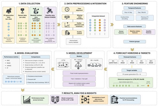
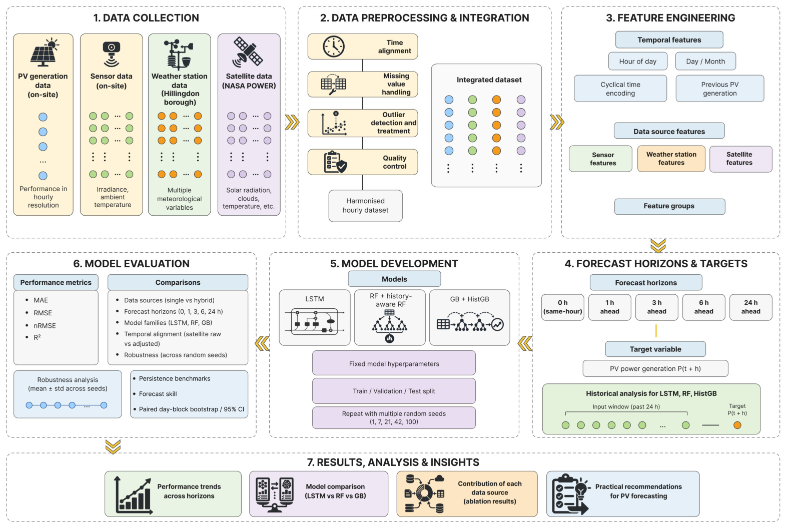
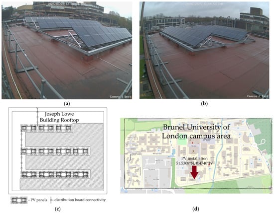
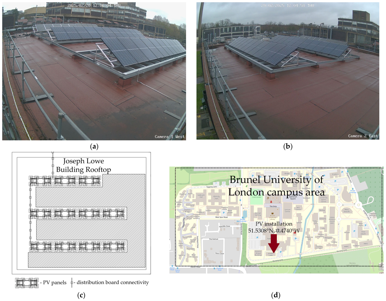
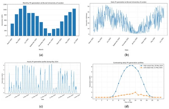
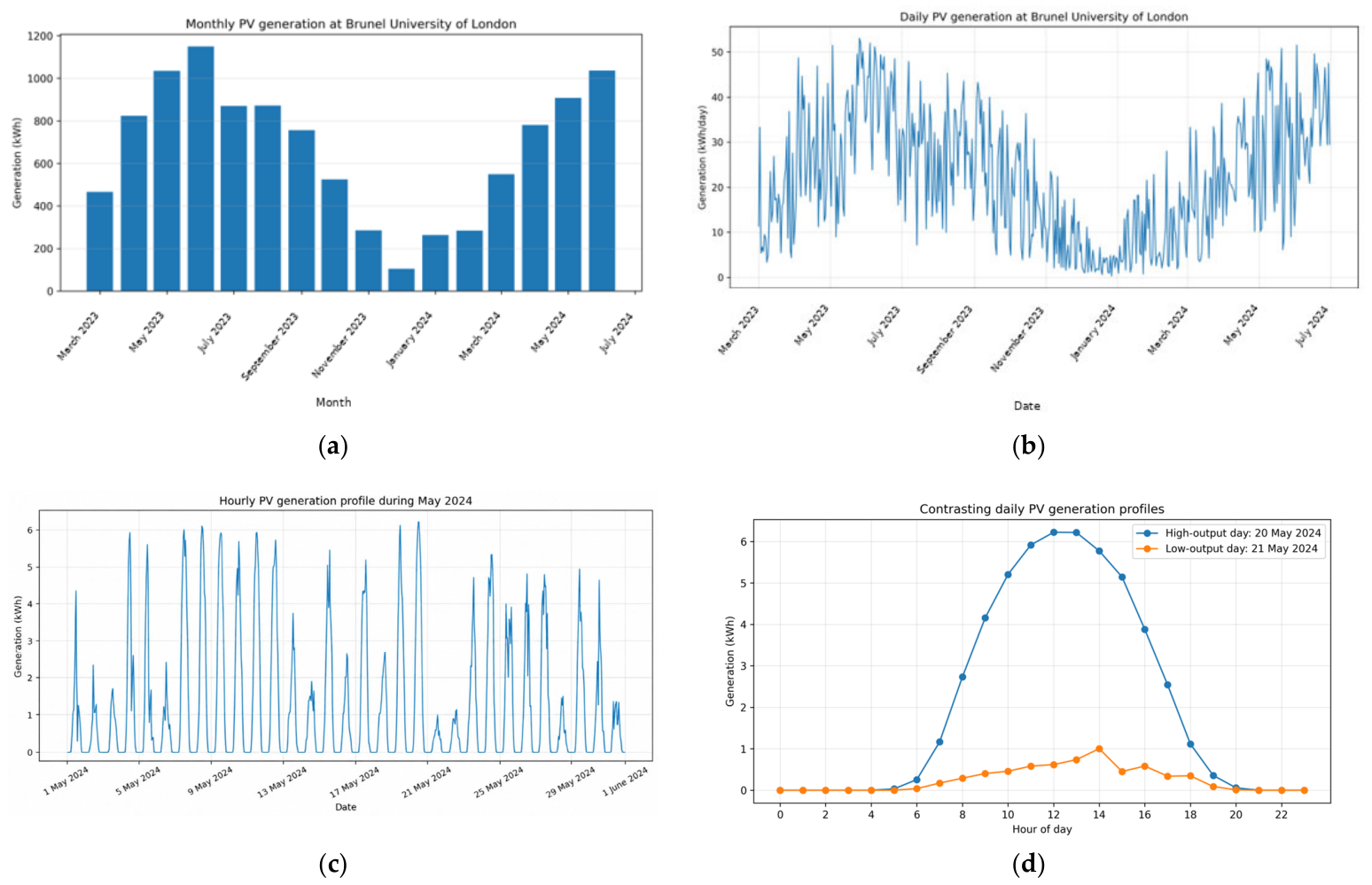
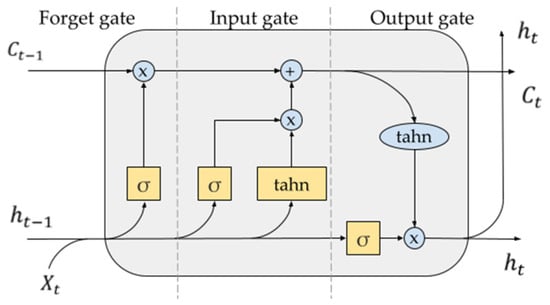
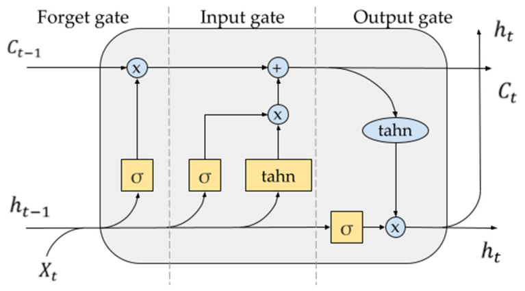
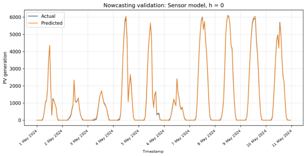
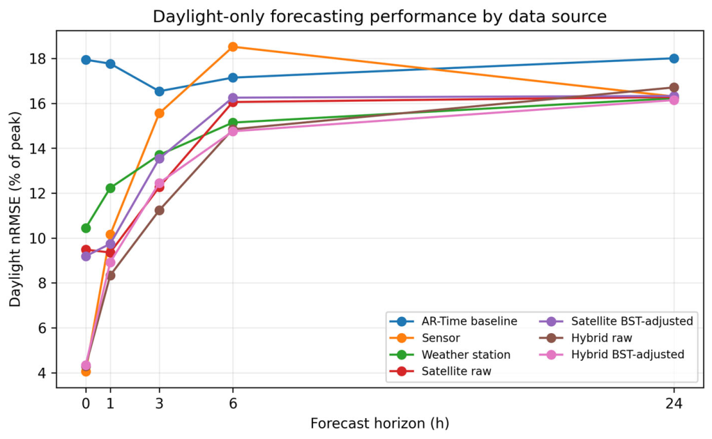
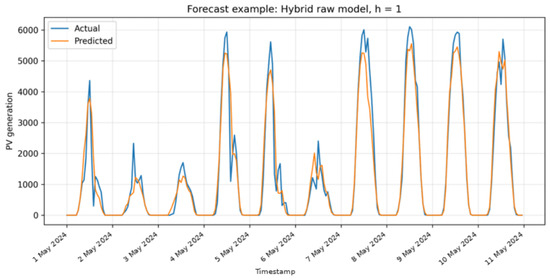
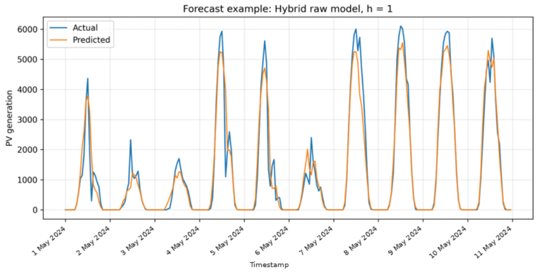
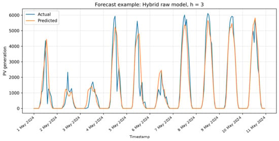
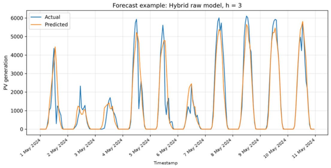
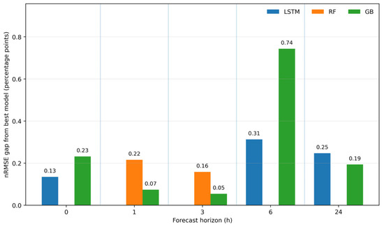
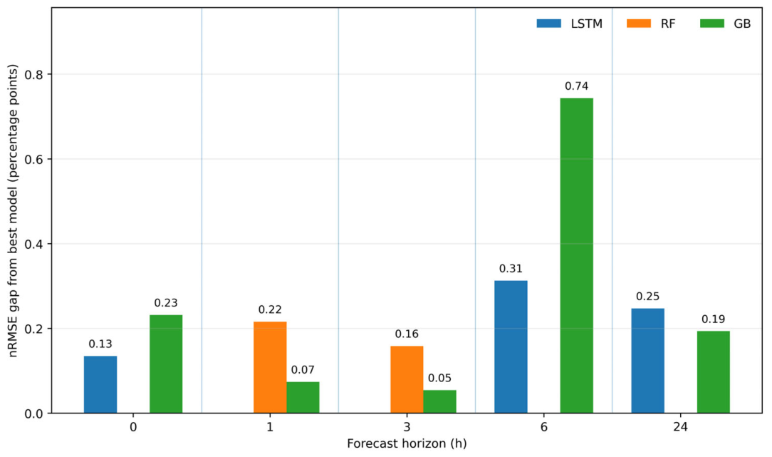
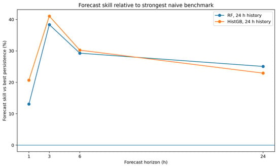
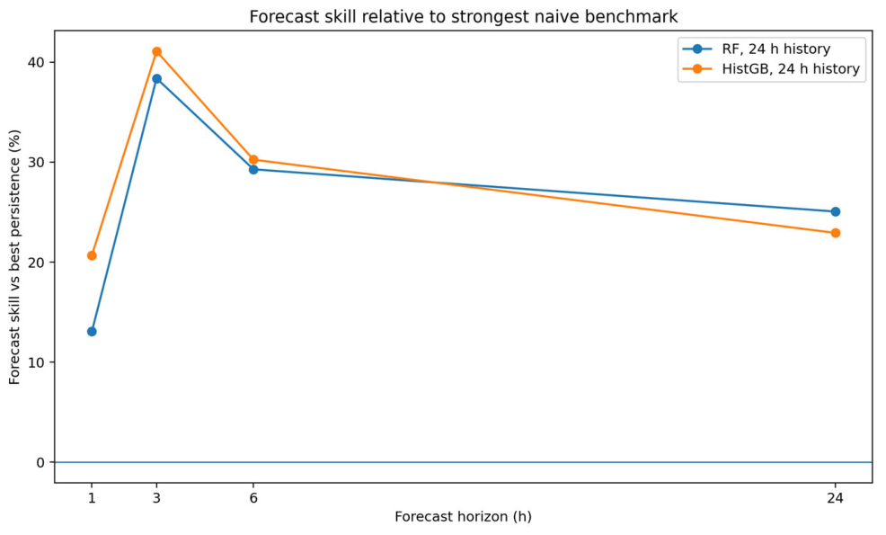

Disclaimer/Publisher’s Note: The statements, opinions and data contained in all publications are solely those of the individual author(s) and contributor(s) and not of MDPI and/or the editor(s). MDPI and/or the editor(s) disclaim responsibility for any injury to people or property resulting from any ideas, methods, instructions or products referred to in the content. |
© 2026 by the authors. Licensee MDPI, Basel, Switzerland. This article is an open access article distributed under the terms and conditions of the Creative Commons Attribution (CC BY) license.