


Abstract
Ultra-deep hydrocarbon formations in northwestern China are critical exploration targets, but their reported measured depths (MD) exceeding 6700 m, low exploration degree, and extremely sparse well control restrict efficient hydrocarbon exploration. Member-level cumulative sandstone thickness provides a measure of sandstone abundance within a stratigraphic member. Conventional methods face difficulties in representing nonlinear relationships between seismic data and cumulative sandstone thickness under sparse well control. To address these problems, this study proposes a CNN-based seismic multi-attribute fusion method for cumulative sandstone thickness prediction in ultra-deep, sparse well areas. Six model inputs were selected empirically with reference to attribute–thickness and inter-attribute Pearson correlations. A geological continuity-constrained augmentation strategy constructs 15 × 15 × 6 multi-channel input patches. The additional patches inherit existing well–member labels and do not add independently measured thickness values. For six well–member units from ss1/wt1, averaging the nine patch predictions for each unit gives MAE = 3.51 m, RMSE = 4.42 m, MSE = 19.51 m2, and R2 = 0.7653. These are descriptive results from only two wells whose labels also informed model selection; they do not establish independent predictive accuracy or spatial generalization. A preliminary interpretation of the predicted thickness patterns, based on the regional geological setting, suggests westward progradation and eastward retrogradation associated with fan delta and braided river delta systems. Areas with predicted cumulative sandstone thicknesses of 30–60 m in interpreted delta front zones are considered potentially favorable exploration targets requiring further petrophysical evaluation. This case study presents a workflow for cumulative sandstone thickness prediction in the studied ultra-deep, well-sparse area; its spatial generalization and applicability beyond the evaluated dataset remain unestablished.
1. Introduction
Ultra-deep hydrocarbon resources have become a major frontier for global oil and gas exploration. With the gradual depletion of shallow and medium-depth resources, exploration has increasingly shifted to ultra-deep strata, which possess enormous resource potential but face severe challenges including complex diagenesis, strong reservoir heterogeneity, extreme burial depth, low exploration degree, and extremely sparse well control [1,2,3]. These conditions lead to great difficulties in reservoir characterization, especially in quantitative prediction of sand body distribution and thickness [4].
Member-level cumulative sandstone thickness can inform geological interpretations of depositional conditions, provenance supply, and sedimentary-system evolution [5,6,7]. In continental sedimentary systems, thick sand bodies developed in fan delta fronts or braided river delta fronts may be favorable exploration targets [8,9]. Sandstone thickness and depositional setting alone are insufficient to establish reservoir quality, which requires independent assessment of petrophysical properties such as porosity and permeability. Therefore, accurate prediction of member-level cumulative sandstone thickness is of great significance for identifying potentially favorable exploration zones, optimizing well locations, and improving exploration success rates.
However, under ultra-deep and sparse well-control conditions, traditional prediction methods are limited by low accuracy, weak generalization, and strong non-uniqueness. Single seismic attributes cannot fully reflect complex geological conditions and often lead to one-sided interpretations [10,11]. Linear multi-attribute fusion ignores multicollinearity and nonlinear relationships, leading to unstable predictions and low reliability [12,13]. Seismic inversion is limited by seismic resolution and non-uniqueness of solutions, and cannot effectively characterize nonlinear relationships between seismic responses and cumulative sandstone thickness [10,14].
In recent years, machine learning and deep learning methods have been widely applied in geophysical prediction and reservoir parameter evaluation driven by seismic data [15]. Convolutional neural networks (CNNs) are particularly suitable for seismic data processing because they can capture spatial features and nonlinear correlations [16,17,18,19]. However, most CNN models require large-scale labeled datasets, which are scarce in ultra-deep frontier exploration areas [20,21]. The use of data augmentation in this setting requires explicit geological assumptions and consideration of dependence among generated samples. These limitations motivate examining workflows for cumulative sandstone thickness prediction under sparse well control. Tian et al. [22] also pointed out that deep learning models integrating multi-dimensional geological constraints can significantly improve the stability and accuracy of reservoir parameter prediction in low-data environments.
To examine an approach under these constraints, this study proposes a CNN-based seismic multi-attribute fusion method integrated with a geological continuity-constrained small-sample augmentation strategy. The main contribution is the integration of neighborhood augmentation based on a local sand-body connectivity assumption with multi-attribute CNN prediction of cumulative sandstone thickness under sparse well control. Empirical attribute selection informed by Pearson correlations and the dual convolutional block CNN serve as established methodological components supporting this workflow. Neighboring samples inherit the thickness label of their source well and member as an approximation, since connectivity alone does not guarantee constant thickness. The workflow is examined as a case study in the available ultra-deep, sparsely drilled study area. Because the evaluation wells also informed model selection, the results do not establish independent predictive accuracy or spatial generalization.
2. Geological Setting and Data
2.1. Tectonic and Sedimentary Setting
The study area is a typical ultra-deep hydrocarbon-bearing sag in northwestern China, located in the central depression zone of a large petroliferous basin [23]. The basin has a typical “north uplift, south gentle tilt” tectonic framework, with multi-stage tectonic activities controlling sedimentary system development [24,25]. The target interval belongs to a Permian clastic succession, which can be subdivided into three members according to sedimentary cycles.
The depositional system is dominated by northwest provenance and supplemented by northeast provenance, forming a fan delta–lacustrine–braided river delta sedimentary assemblage. Sand bodies are mainly developed in the first and third members during regressive stages, while the second member (transgressive stage) is dominated by mudstone with relatively thin sand bodies. Previous exploration indicates hydrocarbon accumulation in delta front sandstones, suggesting exploration potential. The hydrocarbon type in the predicted target areas has not been established in this study. Areas with greater predicted cumulative sandstone thickness are interpreted only as potentially favorable exploration targets requiring independent verification.
2.2. Data Overview and Preprocessing
2.2.1. Seismic Data
Three-dimensional post-stack seismic data with a dominant frequency of approximately 30 Hz and a trace spacing of 25 m × 25 m were used. Seismic interpretation and horizon calibration were completed using Petrel (version 2022). An extraction window extending from 10 ms above the target-member top horizon to 10 ms below its bottom horizon was used to extract 12 seismic attributes related to amplitude, frequency, and energy [26,27,28,29]. Trace spacing describes lateral sampling rather than vertical resolution. An approximate quarter-wavelength benchmark for vertical bed separation is v/(4f), where v is the target-interval P-wave velocity, and f is the dominant frequency [10]. Target-interval P-wave velocity data are available but confidential; their values are not disclosed, so no numerical resolution estimate is reported here. Effective resolution also depends on seismic bandwidth, wavelet shape, and signal-to-noise ratio. The cumulative sandstone thicknesses for Member 3 range from 21 to 58 m and represent summed sandstone interval lengths along the logged well-depth axis, rather than individual-bed vertical thicknesses. Limited bandwidth and thin-bed interference may therefore constrain thickness prediction. The CNN estimates member-level cumulative sandstone thickness from seismic attributes and well labels; its reported accuracy does not demonstrate that individual thin-bed boundaries are resolved.
2.2.2. Well Data
Eight wells with gamma-ray (GR), acoustic, and density logs were used. The reported depth of more than 6700 m refers to measured depth (MD), the distance along the wellbore, rather than true vertical depth (TVD) or true vertical depth below sea level (TVDss). MD alone does not establish source-rock thermal maturity or hydrocarbon-generation stage. Core data were available for all eight wells and covered all three target members of the Fengcheng Formation. Sandstone intervals were identified using a uniform GR < 80 API criterion across all wells and target members, with core observations used for lithologic calibration. This cutoff was used as a study-specific sandstone-identification criterion. The prediction target was the cumulative sandstone thickness within each member of the Fengcheng Formation, calculated by summing the lengths of all interpreted sandstone intervals along the logged measured-depth (MD) axis. Thus, multiple sandstone layers within a member contribute to one thickness label. This lithological total does not represent the thickness of a single sand body or net hydrocarbon pay. Core observations confirm thick sandstone with good sorting, consistent with log interpretation. For Member 3, the eight wells have cumulative sandstone thicknesses of 21–58 m, with a mean of 40.5 m. Core analysis shows that the sandstones are characterized by good sorting and low mud content (<10%), consistent with logging interpretation results. The exact coordinates of the eight wells are not disclosed because of confidentiality restrictions. The CNN predictions complement geological interpretation and do not replace well logging or drilling observations.
3. Methodology
3.1. Overall Workflow
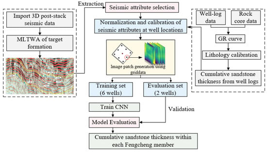
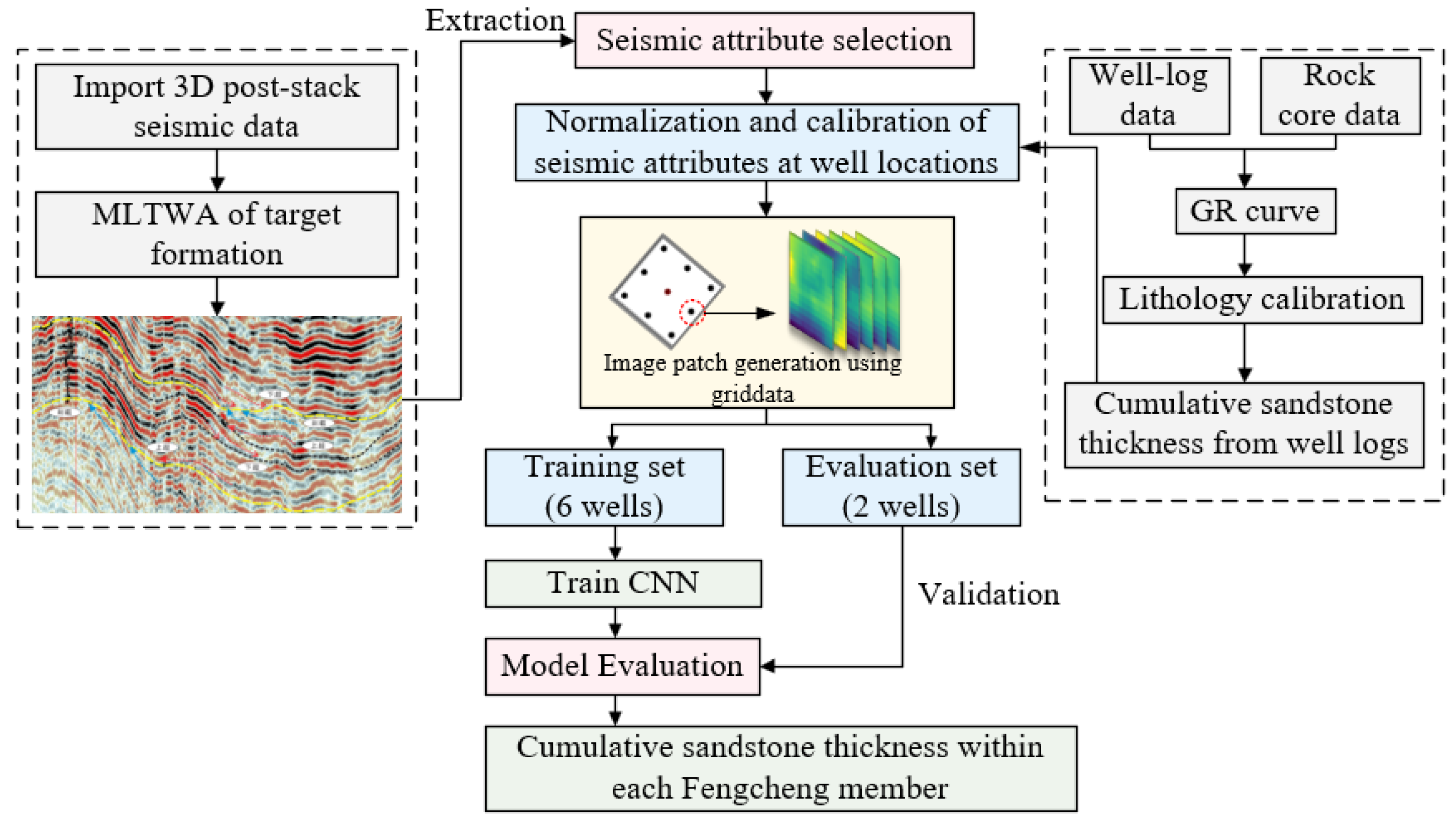
The overall workflow includes four steps (Figure 1):
Figure 1.
Workflow of CNN-based cumulative sandstone thickness prediction, including seismic attribute selection, well-log and core calibration, sample construction, model training, and evaluation. The two-well evaluation subset also supplies the labels used for early stopping and selection of the restored weights; it is not an independent final test set.
- •
- Seismic attribute extraction and empirical selection informed by Pearson correlation analysis.
- •
- Data preprocessing (normalization, invalid-data screening, spatial matching);
- •
- Sample construction and augmentation (neighborhood sampling and spatial interpolation);
- •
- CNN model training, joint validation/model selection and evaluation, and cumulative sandstone thickness prediction.
3.2. Seismic Attribute Selection
Pearson correlation coefficient (r) was used to quantify the linear relationship between the 12 extracted seismic attributes and cumulative sandstone thickness, as well as the mutual correlation among seismic attributes [30]. Attribute–thickness and inter-attribute correlations were calculated from matched observations from all eight wells across the three members, including ss1 and wt1. The ss1/wt1 thickness labels therefore contributed to attribute selection, which was not confined to the six training wells. The correlation coefficients between the 12 candidate seismic attributes and cumulative sandstone thickness are presented in Table 1, while the pairwise correlations among the six selected seismic attributes are shown in Table 2. The two tables provide descriptive correlations that informed the empirical selection of the six-attribute input set. No fixed numerical exclusion threshold or formal mathematical optimization was applied. The empirical input set comprised six seismic attributes: root mean square amplitude (RMS, r = 0.790), amplitude asymmetry (AA, r = 0.788), energy half-time (EHT, r = 0.721), maximum absolute amplitude (MAA, r = 0.637), average absolute amplitude (AAA, r = 0.438), and total energy (TE, r = 0.287). Total energy (TE) was retained empirically as an energy-related descriptor within the six-attribute input set, despite its lower correlation with cumulative sandstone thickness (r = 0.287) and its correlation with MAA (r = 0.6469). The independent predictive contribution of TE has not been established. Pairwise correlation was used as a preliminary assessment of linear redundancy, rather than as a complete multicollinearity diagnosis. As an additional descriptive diagnostic, approximate variance inflation factors (VIFs) were derived as the diagonal entries of the inverse of the six-attribute correlation matrix in Table 2. This matrix was calculated from the same complete paired observations from eight wells across the three members. Using the rounded coefficients reported in Table 2, the approximate VIFs are 2.25 (RMS), 1.68 (AAA), 2.22 (MAA), 1.76 (TE), 1.19 (AA), 1.19 (EHT). These estimates were derived from rounded coefficients rather than recalculated from raw attribute data, and their precision is limited by rounding. They provide an approximate descriptive check of linear redundancy in the existing input set, not a diagnostic confined to the training data or evidence of an optimal attribute combination. They do not establish the absence of nonlinear dependence or independent predictive contributions of individual inputs. These six attributes describe amplitude and energy characteristics and were used as the input parameters for the subsequent CNN model.
Table 1.
Pearson correlation coefficients between the 12 candidate seismic attributes and cumulative sandstone thickness, using matched observations from all eight wells, including ss1 and wt1.
Table 2.
Pairwise Pearson correlation coefficients among the six selected seismic attributes, using matched observations from all eight wells, including ss1 and wt1.
3.3. Data Preprocessing
Data quality directly determines the reliability and upper limit of model performance. To ensure the representativeness and consistency of input attributes, multiple seismic attribute datasets were subjected to unified preprocessing and calibration procedures. Each seismic attribute was linearly mapped to [0, 1] using its minimum and maximum values over the study-area seismic attribute data. The same global ranges were used for training and evaluation inputs; the normalization parameters were not estimated exclusively from the six training wells. The scaling parameters depend on seismic input values rather than measured thickness labels, but their use of full-study-area extrema means that normalization was not isolated from the evaluation inputs. This scaling places attributes with different numerical ranges on a comparable scale. Data quality control identified runs of more than seven consecutive null entries, and the corresponding invalid data points were excluded. Nearest-neighbor interpolation was used to fill the resulting gaps and other missing attribute values. The number of excluded data points and interpolated values was not quantified, which limits quantitative auditing of preprocessing. Generated patches were subsequently screened using the criterion for the proportion of filled grid points described in Section 3.4.
Well-based cumulative sandstone thickness values were spatially matched with the extracted seismic attributes at the well locations. Table 3 presents the matched Member 3 data for the eight wells as an example, including cumulative sandstone thickness and the six selected seismic attribute values for each well. The matched observations form the original labeled data for subsequent model training and sample augmentation.
Table 3.
Cumulative sandstone thickness (CST) and matched seismic attributes for Member 3. CST is reported in m.
3.4. Small-Sample Augmentation Strategy
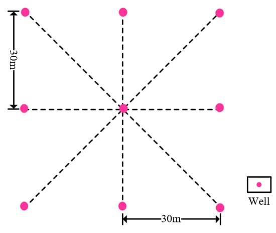
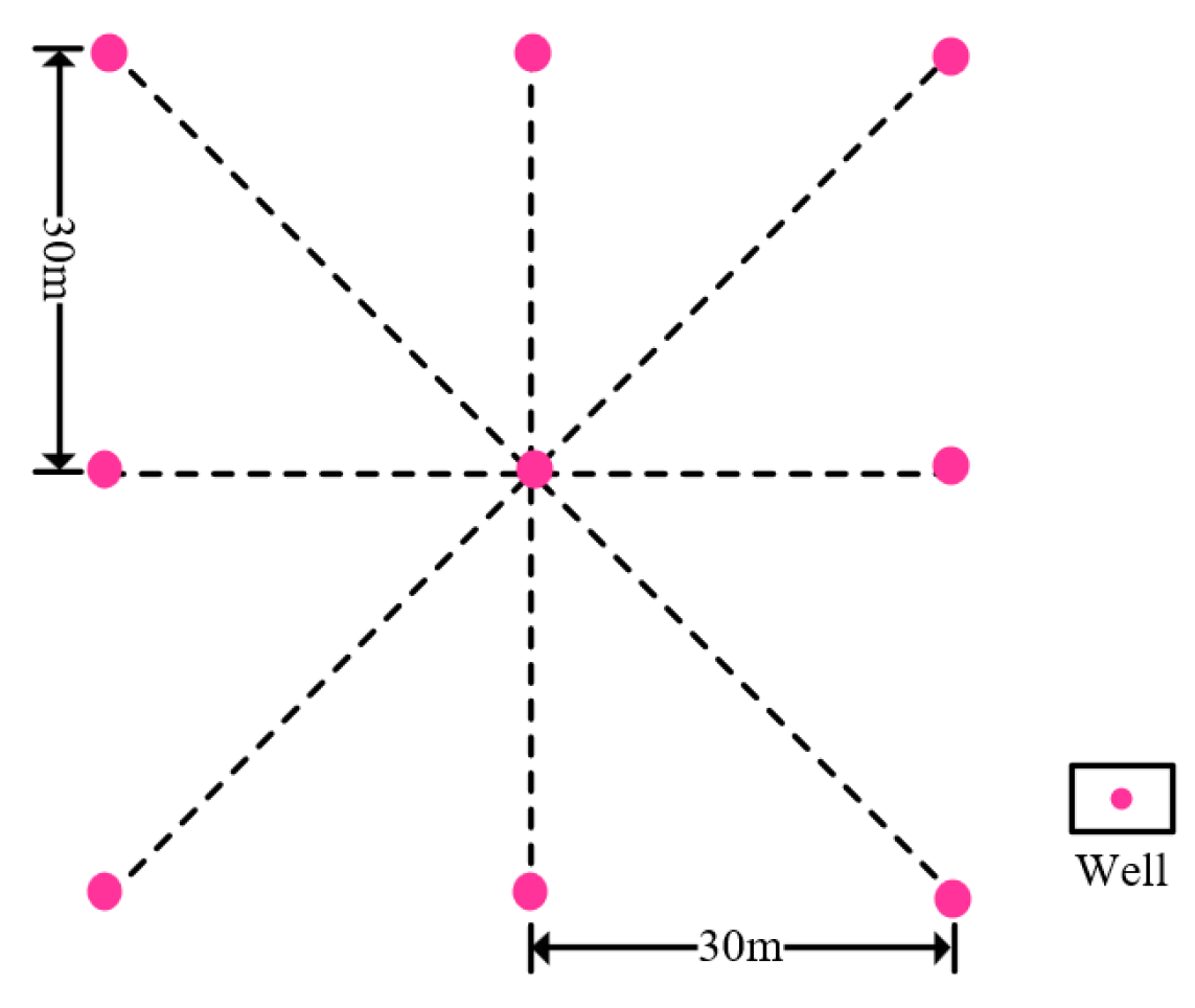
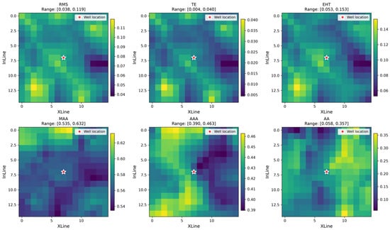
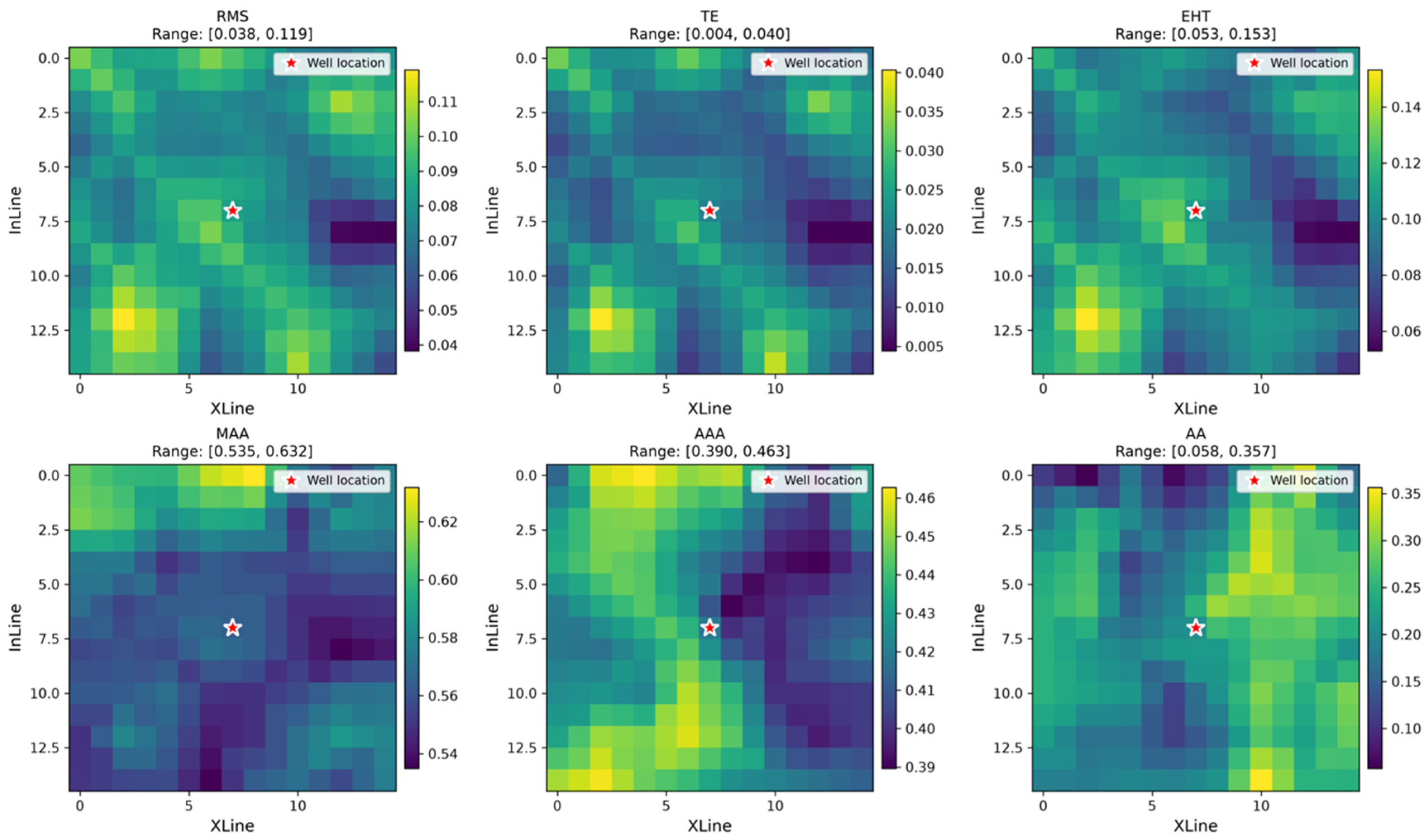
The computational workflow was implemented in Python (version 3.9.18), using TensorFlow (version 2.10.0), NumPy (version 1.26.4), pandas (version 2.3.2), SciPy (version 1.13.1), and scikit-learn (version 1.6.1). A geological continuity-constrained augmentation strategy was proposed (Figure 2). Neighborhood sampling and spatial interpolation were used under a local sand-body connectivity assumption. This assumption provides the basis for assigning the well-center thickness to neighboring locations within the same member. For each well and member, a 3 × 3 set of sampling centers comprised the well center and eight neighboring locations. Adjacent centers were separated by three sampling steps along each sampling direction, corresponding to the physical separation of 30 m shown in Figure 2. Seismic attribute features were extracted around each sampling center, and all nine locations for a given well and member were assigned the cumulative sandstone thickness label at the well center, providing the thickness labels for the augmented samples. Each sample retained its source-well and member identity. These augmented inputs were derived from eight source wells and do not represent 216 independent well observations. The inherited label is an approximation: connectivity does not guarantee constant thickness, and the assumption may fail near faults, facies boundaries, or rapid thickness changes. Neighboring patches may share thickness labels and overlapping seismic information. As specified in Section 3.6, all samples derived from a source well belong exclusively to one subset. This keeps source-well membership distinct between the training and joint validation/evaluation subsets, but does not remove dependence among neighboring samples or make the final evaluation independent of model selection. Subsequently, an image-patch generation method based on spatial interpolation was applied. Using the griddata function from the SciPy library (version 1.13.1), each sampling center was used to construct a 15 × 15-pixel image patch with six seismic attribute channels (15 × 15 × 6). The 3 × 3 layout defines the sampling-center locations, whereas 15 × 15 defines the pixel grid within each patch. For blank regions at the boundaries, the mean values of neighboring data points were used for filling. Finally, patches were screened using the proportion of filled grid points. This proportion was defined as the number of originally missing grid points that received filled values divided by the 225 grid points in a 15 × 15 patch. It was calculated after missing-value filling by counting the points that had been filled, rather than the remaining missing entries. Patches with this proportion below 0.3 were retained, meaning that fewer than 30% of their grid points had received filled values. The final dataset comprised 216 patches after this screening (eight wells × three members × nine neighborhood samples). A typical multi-channel sample example is displayed in Figure 3. The augmentation increases the number of local input patches without adding independently measured thickness labels.
Figure 2.
Schematic diagram of geological continuity-constrained small-sample augmentation.
Figure 3.
Example of 15 × 15 × 6 multi-channel training samples constructed from empirically selected seismic attributes. The star marks the well location.
3.5. CNN Model Architecture
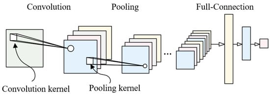
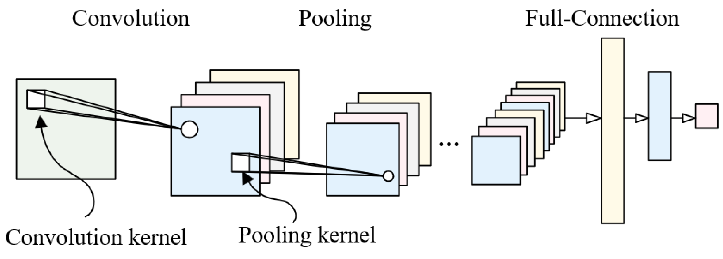
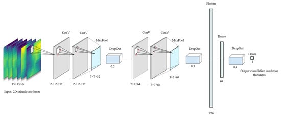
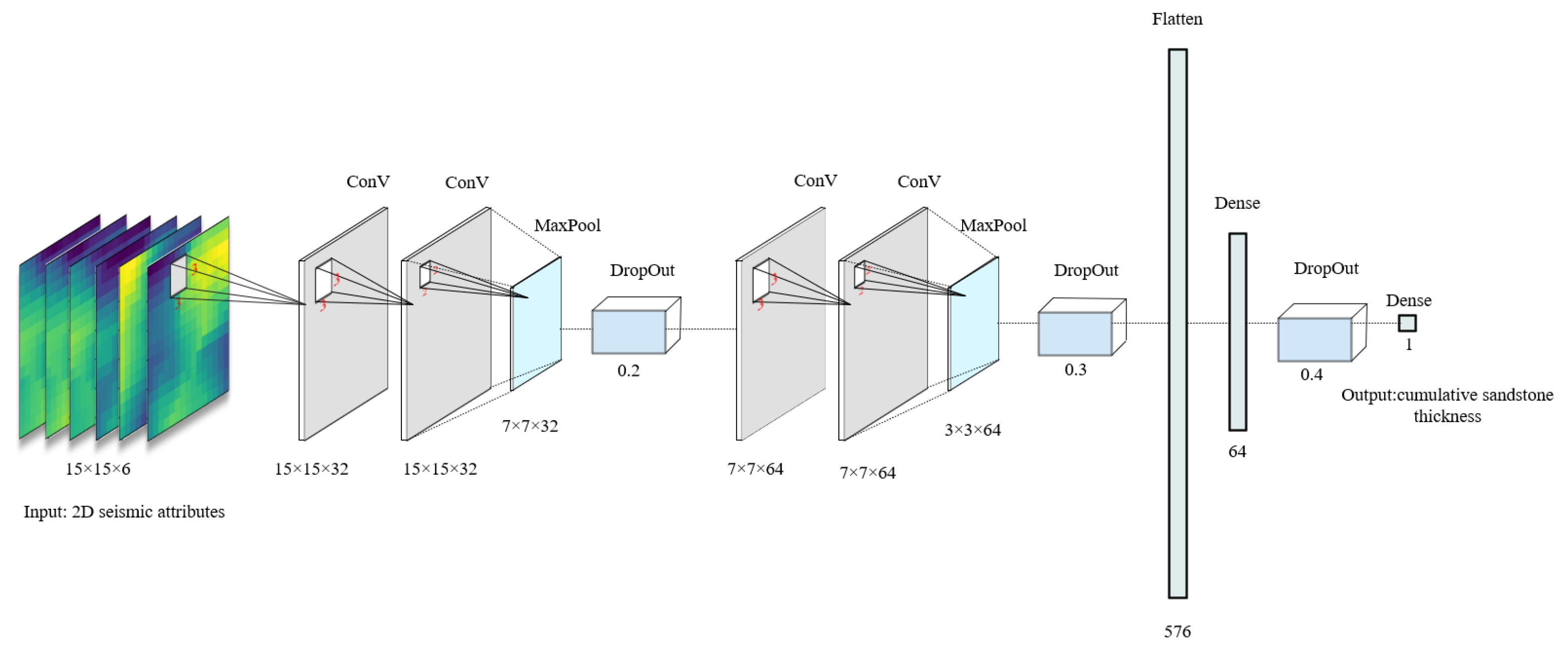
The CNN model was designed to capture spatial structural features of seismic attributes, with a dual convolutional block architecture (Figure 4):
Figure 4.
Architecture of the proposed dual convolutional block CNN model.
- •
- Input layer: 15 × 15 × 6 multi-channel seismic attributes (normalized to [0, 1] to eliminate dimensional differences);
- •
- Convolutional Block 1: Two 3 × 3 convolutional layers (32 kernels each) with ReLU activation, followed by 2 × 2 max-pooling (downsampling to 7 × 7) and dropout (rate = 0.2);
- •
- Convolutional Block 2: Two 3 × 3 convolutional layers (64 kernels each) with ReLU activation, followed by 2 × 2 max-pooling (downsampling to 3 × 3) and dropout (rate = 0.3);
- •
- Fully connected layers: Flattened 3 × 3 × 64 features (576 dimensions) → 64-dimensional vector (ReLU activation, dropout rate = 0.4) → 1-dimensional output (member-level cumulative sandstone thickness);
- •
- Loss function: Mean squared error (MSE); Optimizer: Adam (learning rate = 0.001, batch size = 32, maximum epochs = 100). The learning rate, batch size, dropout rates, and network architecture were set empirically, without a systematic hyperparameter search.
The model extracts multi-scale spatial features, with dropout used for regularization. Early stopping monitored validation MSE (val_loss) and stopped training after 10 consecutive epochs without improvement (patience = 10). The weights from the epoch with the lowest validation MSE were restored (restore_best_weights = True). Training stopped before reaching the 100-epoch limit. The same 54 patches from ss1 and wt1 formed the subset used jointly for validation/model selection and evaluation. Their labels informed the stopping epoch and selection of the restored weights. No separate validation subset or untouched final test set was used. The well–member-level assessment described in Section 3.6 uses these same source wells and does not constitute an independent final-test evaluation. Detailed network parameters are shown in Figure 5.
Figure 5.
Detailed configuration and parameter settings of the CNN model.
3.6. Model Evaluation Indicators
Four statistical indicators were used to evaluate model performance [6]:
- •
- Mean Absolute Error (MAE): Measures the mean absolute prediction error, reported in m.
- •
- Mean Squared Error (MSE): Measures the mean squared prediction error, reported in m2 and sensitive to large errors.
- •
- Root Mean Squared Error (RMSE): The square root of MSE, reported in m, with greater sensitivity to large errors than MAE.
- •
- Coefficient of Determination (R2): A dimensionless measure of agreement between predicted and observed values within the evaluated dataset, interpreted in the context of the dataset’s size and independence.
The dataset was partitioned by source well into a training subset and a subset used jointly for validation/model selection and evaluation. Wells tt1, sp7, zj1, zs1, zt1, and zt2 were assigned to training, giving six training wells (75%), while ss1 and wt1 formed the joint validation/evaluation subset, giving two evaluation wells (25%). All samples from a given well, including all three members and the nine neighborhood samples per member, belonged exclusively to the same subset. Each well contributed 27 patches, yielding 162 training patches and 54 patches in the joint validation/evaluation subset. Source-well membership determined the allocation; individual patches were not randomly assigned across the two subsets. The ss1/wt1 labels supplied the validation MSE monitored during early stopping and informed selection of the restored model weights. No separate validation subset or untouched final test set was used. Thus, grouping by source well does not make this evaluation independent of model selection, and the reported well–member-level metrics summarize predictions derived from the reused ss1/wt1 subset. The source-well split did not isolate attribute selection or normalization from the evaluation data (Section 3.2 and Section 3.3).
For the descriptive evaluation reported here, the nine patch predictions belonging to each well and member are averaged to obtain one predicted cumulative sandstone thickness. This mean is paired with the corresponding measured thickness label from the central well. The 54 patches therefore yield six well–member pairs (two wells × three members), rather than 54 independent geological observations. MAE and MSE are calculated from the six differences between mean predicted and observed thickness; RMSE is the square root of this MSE. R2 is calculated using the summed squared errors of these six pairs relative to the summed squared deviations of their observed values from the six-value observed mean. All six units receive equal weight. These reported metrics are distinct from the patch-level validation MSE used during early stopping. The six units are clustered within two wells and are not assumed to be statistically independent. Given the small, reused dataset, R2 is interpreted in the context of the number and dependence of the evaluated units, without applying a universal performance threshold. Interpretation emphasizes MAE, RMSE, and direct observed–predicted comparisons.
4. Practical Application and Results
4.1. Model Performance Evaluation
As described in Section 3.6, six wells supplied the training subset, and ss1/wt1 supplied the subset used jointly for validation/model selection and evaluation. Table 4 presents observed cumulative sandstone thickness, the mean of the nine patch predictions, and the corresponding error for each of the six well–member units. These units are clustered within two wells; the 54 patches do not represent 54 independent geological observations.
Table 4.
Observed and mean predicted cumulative sandstone thickness for the six well–member units.
Across the six displayed pairs, MAE = 3.51 m, RMSE = 4.42 m, MSE = 19.51 m2, and R2 = 0.7653. The largest absolute error is 9.156 m for wt1 Member 3 (observed 21 m; mean predicted 30.156 m); the other five absolute errors range from 1.017 to 3.568 m. These values are descriptive summaries of the six pairs, and R2 should be interpreted cautiously because the units are few and clustered within only two wells. The same source-well labels also informed early stopping and selection of the restored weights. Aggregation does not remove this reuse: the results do not constitute an independent final test or establish spatial generalization.
4.2. Predicted Cumulative Sandstone Thickness Distribution
4.2.1. Distribution Across the Three Members
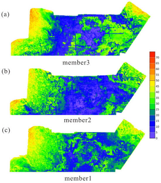
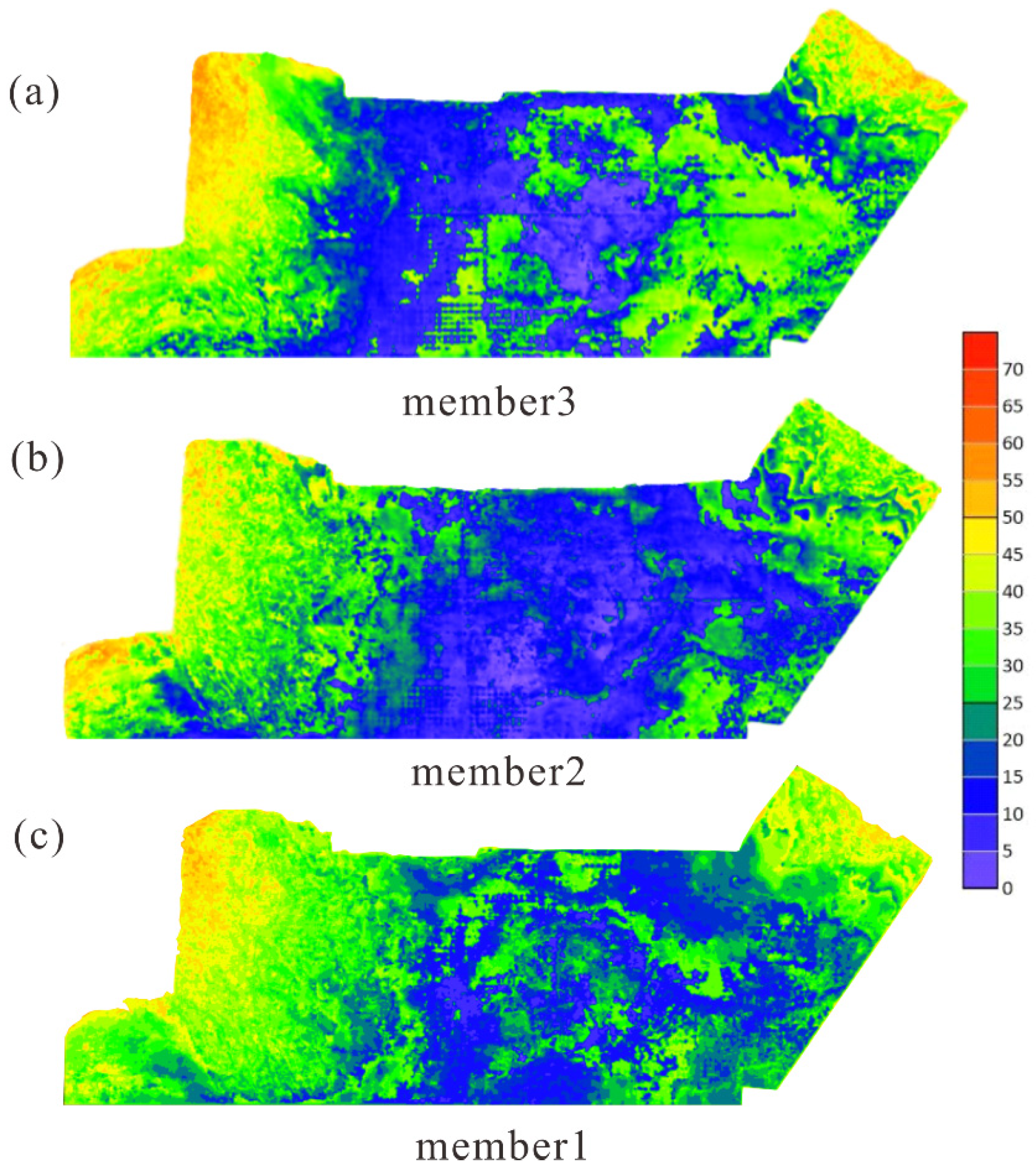
The CNN predicts member-level cumulative sandstone thickness. The thickness maps show spatial variation in this cumulative quantity; they do not delineate the boundaries or three-dimensional geometry of individual sand bodies. The depositional stages, facies, and evolutionary processes discussed in Section 4.2, Section 4.3 and Section 5.1 are preliminary interpretations of these thickness patterns in the regional geological context described in Section 2.1; they are not direct CNN outputs and have not been independently verified. Member 1 (Initial transgressive stage): Predicted cumulative sandstone thicknesses of 25–50 m occur over broad areas, with tongue-shaped or wedge-shaped spatial patterns (Figure 6c). Within this geological context, tectonic activity and multiple sediment sources are interpreted to have favored fault-controlled fan deltas.
Figure 6.
Predicted cumulative sandstone thickness distributions for the three target members: (a) Member 3; (b) Member 2; (c) Member 1. The shared color scale shows predicted cumulative sandstone thickness (m).
Member 2 (Peak transgressive stage): Predicted cumulative sandstone thickness has values of 15–30 m (Figure 6b), interpreted in the regional evolutionary context as corresponding to peak lake level and expanded deep-water areas. Areas with greater predicted cumulative sandstone thickness are tentatively attributed to transport through subaqueous distributary channels.
Member 3 (Regressive stage): The predicted cumulative sandstone thickness pattern (30–60 m; Figure 6a) is tentatively interpreted as westward progradation and eastward retrogradation. Southward migration of the sedimentary center and multi-stage lobe development along the northwest steep slope are interpretations within the regional evolutionary context, rather than direct model predictions.
4.2.2. Lateral Distribution Characteristics
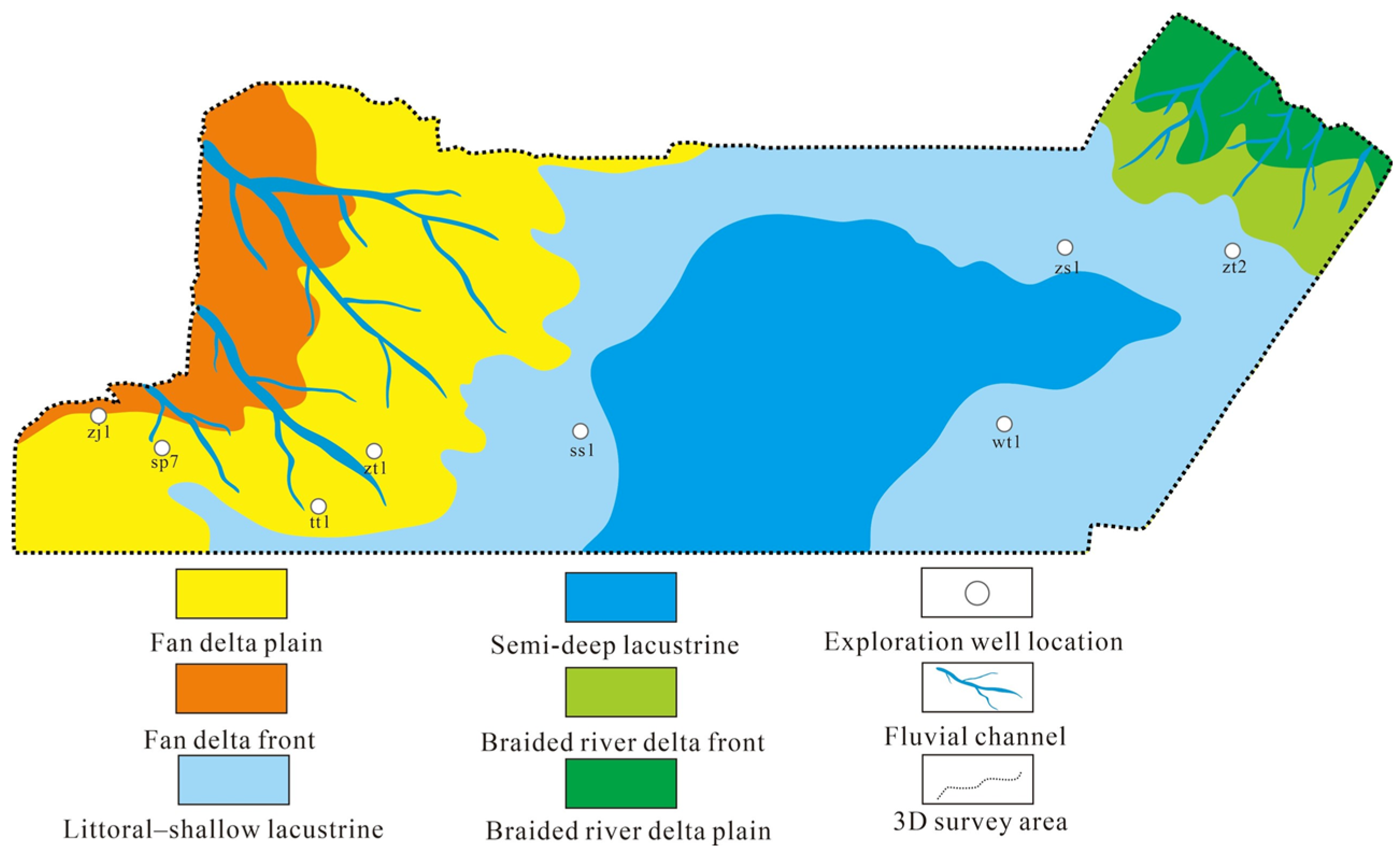
Predicted cumulative sandstone thickness shows a “thicker in west and north, thinner in east and south” pattern (Figure 6). In this preliminary facies interpretation, the northwest is assigned mainly to fan delta plain and front facies (predicted cumulative thickness of 40–60 m), the northeast to braided delta front facies (30–45 m), and the central and eastern areas to littoral–shallow lacustrine and semi-deep lacustrine facies (<25 m).
4.3. Potentially Favorable Exploration Zones
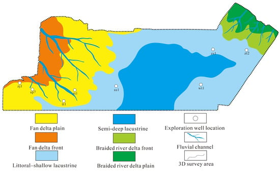
Areas with predicted cumulative sandstone thicknesses of 30–60 m in interpreted delta front zones are considered potentially favorable exploration targets (Figure 7). Predicted thickness and depositional setting alone do not establish porosity, permeability, or reservoir quality. Independent porosity and permeability data are needed to evaluate reservoir quality in these zones.
Figure 7.
Preliminary interpretation of sedimentary distribution and potentially favorable exploration zones from predicted cumulative sandstone thickness patterns.
5. Discussion
5.1. Geological Interpretation of Cumulative Sandstone Thickness Patterns
Within the regional geological framework described in Section 2.1, the predicted spatial distribution of cumulative sandstone thickness within the Fengcheng Formation members is tentatively interpreted in relation to three factors:
- •
- Tectonic setting: The “north uplift, south gentle tilt” framework may influence provenance direction and sedimentary center migration.
- •
- Provenance supply: The northwest DBS Uplift is the main provenance, providing abundant clastic material, while the northeast provenance supplements.
- •
- Lake-level fluctuations: Transgressive-regressive cycles are interpreted as influencing vertical sand body development, with regressive stages favoring thick sand body accumulation.
5.2. Methodological Comparison with Traditional Methods
Post-stack model-constrained acoustic impedance inversion estimates sandstone distribution through a well-calibrated relationship between lithology and acoustic impedance, whereas single-attribute linear regression relates RMS to cumulative sandstone thickness. The present CNN workflow combines multiple attributes and spatial input patches. Corresponding well–member-level predictions from the two baseline methods are not available for a comparison on the same six-pair basis; therefore, no quantitative advantage over these methods is established here. The following comparison concerns methodological components, whose individual predictive benefits have not been independently demonstrated:
- •
- Nonlinear modeling of the relationship between seismic attributes and cumulative sandstone thickness.
- •
- Neighborhood augmentation of input patches under a geological continuity assumption, without adding independently measured thickness labels.
- •
- Convolution operations that encode spatial patterns within multi-attribute seismic patches. These components describe the workflow; the current evaluation does not independently establish their predictive benefits or the superiority of the CNN.
5.3. Limitations and Future Work
The existing model is retained in this case study, and interpretation is restricted to the jointly used dataset. The 54 patches from ss1 and wt1 were used to monitor early stopping and select the restored weights; the reported performance is now summarized using six well–member mean predictions derived from those patches. No separate validation set or untouched final test set was used. This reuse makes the reported metrics descriptive results on a dataset used jointly for model selection and evaluation, and they may be optimistic. They do not establish independent predictive accuracy, spatial generalization, or an independently tested advantage over the baseline methods. No additional wells with matched seismic attributes and measured cumulative sandstone thickness labels from the Fengcheng Formation in the study area are currently available to us for external validation. This data limitation does not resolve the lack of an independent final test.
Only eight source wells were available, and the six-well training subset and two-well joint validation/evaluation subset provide limited geological coverage. Augmentation increases the number of input patches without adding independently measured thickness labels. Augmented patches from the same well and member share the original thickness label and may contain overlapping seismic information; consequently, the 54 evaluation patches do not represent 54 independent observations. Their aggregation yields six well–member units clustered within only two wells, not six statistically independent wells or sites. The direct comparisons and error magnitudes in Table 4 should be emphasized, and the six-pair R2 should be interpreted cautiously. Grouping all samples by source well prevents the same well from contributing to both subsets, but spatial correlation among samples may persist, and this grouping does not ensure independence from model selection.
Attribute selection used correlations from all eight wells, including the ss1/wt1 thickness labels, while normalization used minima and maxima from the full study-area seismic attribute data. Thus, feature selection and preprocessing were not fully separated from the data subsequently used for evaluation. The VIF values are approximate estimates from rounded all-well correlations, not values recalculated from raw training data. Evidence from with-versus-without TE comparisons or feature-importance analysis is not provided here. Consequently, the incremental predictive contribution of TE and the optimality of the six-attribute input set remain unestablished. The effects of these shared procedures on the reported metrics have not been quantified.
Future independent evaluation should derive attribute selection, raw-data redundancy diagnostics, and normalization parameters from training data, use well-grouped validation for model selection, and reserve untouched wells for final testing with the fixed preprocessing applied unchanged. Applicability beyond the evaluated dataset, including areas with similar geological conditions, remains unestablished. Application to another area requires independent validation and locally appropriate attribute selection and model construction. Future work could examine structural constraints, diagenetic parameters, and 3D CNN architectures through independent evaluation.
Limitations include sensitivity to strong tectonic deformation and incomplete consideration of diagenesis. All exploration implications drawn from the predicted cumulative sandstone thickness patterns are limited to identifying potentially favorable exploration targets. Cumulative sandstone thickness alone does not confirm hydrocarbon presence, type, or recoverability. No economic evaluation is presented in this study. Drilling and operating costs require a separate assessment before commercial viability can be evaluated. Quantitative evidence of well spacing and coverage of formation boundaries is not provided here. Predictions in areas with limited well control, including any extrapolation, should therefore be treated cautiously and independently verified using geological and well observations.
6. Conclusions
- (1)
- Six seismic attributes were selected empirically with reference to attribute–thickness and inter-attribute correlations calculated from all eight wells. This input set was not established through formal mathematical optimization.
- (2)
- The geological continuity-constrained augmentation strategy expands the local seismic input-patch set through neighborhood sampling. The additional patches inherit existing well–member labels and do not add independently measured thickness values. An independent predictive benefit from augmentation has not been established here.
- (3)
- For the six well–member units from ss1/wt1, nine-patch mean predictions yield MAE = 3.51 m, RMSE = 4.42 m, MSE = 19.51 m2, and R2 = 0.7653. These values describe only six units clustered within two wells whose labels also informed model selection. R2 should be interpreted cautiously; the results do not constitute an independent final-test evaluation, establish spatial generalization, or demonstrate a quantitative advantage over the baseline methods.
- (4)
- A preliminary interpretation of predicted thickness patterns in the regional geological context suggests progradation and retrogradation, and areas with greater predicted cumulative sandstone thickness in interpreted delta front zones are considered potentially favorable exploration targets requiring petrophysical evaluation.
- (5)
- This case study presents a CNN-based workflow for cumulative sandstone thickness prediction under the available ultra-deep, sparse well-control conditions. Its predictive accuracy at independent wells and applicability beyond the evaluated dataset remain unestablished and require independent validation, together with attribute selection and model construction adapted to local geology.
Author Contributions
Methodology, G.L. and X.C.; Software, Y.S. and X.C.; Validation, X.L. and Q.C.; Formal analysis, X.L.; Writing—original draft, Y.S.; Writing—review and editing, G.L.; Visualization, G.L.; Project administration, G.L.; Funding acquisition, G.L. All authors have read and agreed to the published version of the manuscript.
Funding
This research was funded by the Shandong Provincial Natural Science Foundation of China, grant number ZR2021MD061.
Data Availability Statement
The codebase is maintained within the research framework. To facilitate reproducibility, the manuscript documents the key architectural, training, and evaluation details of the proposed method. Data requests may be directed to the corresponding author, subject to applicable confidentiality restrictions and authorization requirements.
Conflicts of Interest
The authors declare no conflicts of interest.
References
- Sun, J.; You, X.; Zhang, Q.; Xue, J.; Chang, Q. Development characteristics and genesis of deep tight conglomerate reservoirs of Mahu area in Junggar Basin, China. J. Nat. Gas Geosci. 2023, 8, 201–212. [Google Scholar] [CrossRef] [Scilit]
- Dang, W.-L.; Gao, G.; You, X.-C.; Fan, K.-T.; Wu, J.; Lei, D.-W.; He, W.-J.; Tang, Y. Geochemical identification of a source rock affected by migrated hydrocarbons and its geological significance: Fengcheng Formation, southern Mahu Sag, Junggar Basin, NW China. Pet. Sci. 2024, 21, 100–114. [Google Scholar] [CrossRef] [Scilit]
- Fu, X.; Zhang, F.; Cao, D. Joint PP and PS seismic inversion using predicted PS waves from deep learning. Pet. Sci. 2025, 22, 4573–4583. [Google Scholar] [CrossRef] [Scilit]
- Tan, F.; Yang, P.; Cao, J.-X.; Li, L.; Cui, Z.; Ma, Q. Challenges and solutions to seismic amplitude pitfalls in dim-spot sandstone reservoirs: A case study from the Shaximiao formation, the Western Sichuan Depression, China. J. Appl. Geophys. 2026, 244, 106016. [Google Scholar] [CrossRef] [Scilit]
- Li, H.; Gao, R.; Wang, Y. Predicting the thickness of sand strata in a sand-shale interbed reservoir based on seismic facies analysis. J. Geophys. Eng. 2020, 17, 592–601. [Google Scholar] [CrossRef] [Scilit]
- Zhen, Y.; Zhang, A.; Zhao, X.; Ge, J.; Zhao, Z.; Yang, C. Prediction of deep low permeability sandstone seismic reservoir based on CBAM-CNN. Geoenergy Sci. Eng. 2024, 242, 213241. [Google Scholar] [CrossRef] [Scilit]
- Zhen, Y.; Zhao, Z.; Zhao, X.; Ge, J.; Zhang, A.; Yang, C. Method and application of sand body thickness prediction based on virtual sample machine learning. Geophysics 2024, 89, M169–M184. [Google Scholar] [CrossRef] [Scilit]
- Lan, N.-Y.; Zhang, F.-C.; Sang, K.-H.; Yin, X.-Y. Simultaneous denoising and resolution enhancement of seismic data based on elastic convolution dictionary learning. Pet. Sci. 2023, 20, 2127–2140. [Google Scholar] [CrossRef] [Scilit]
- Zhang, X.; Zhang, C.; Yang, W.; Zhu, R.; Fu, W. Sedimentary characteristics and quantification of a distributive fluvial system: A case study of the Jurassic Shaximiao Formation in the Northwest Sichuan Basin. Acta Sedimentol. Sin. 2025. [Google Scholar] [CrossRef]
- Puryear, C.I.; Castagna, J.P. Layer-thickness determination and stratigraphic interpretation using spectral inversion: Theory and application. Geophysics 2008, 73, R37–R48. [Google Scholar] [CrossRef] [Scilit]
- Oumarou, S.; Mabrouk, D.; Tabod, T.C.; Marcel, J.; Iii, S.N.; Essi, J.M.A.; Kamguia, J. Seismic attributes in reservoir characterization: An overview. Arab. J. Geosci. 2021, 14, 402. [Google Scholar] [CrossRef] [Scilit]
- Subrahmanyam, D.; Rao, P.H. Seismic attributes-A review. In Proceedings of the 7th International Conference and Exposition on Petroleum Geophysics, Hyderabad, India, 14–16 January 2008; pp. 398–404. [Google Scholar]
- Wang, X. Reservoir prediction and application of multi-attribute fusion. IOP Conf. Ser. Earth Environ. Sci. 2021, 651, 032072. [Google Scholar] [CrossRef] [Scilit]
- Xu, S.-G.; Bao, Q.-Z.; Ren, Z.-M. Target-oriented Q-compensated reverse-time migration by using optimized pure-mode wave equation in anisotropic media. Pet. Sci. 2023, 20, 866–878. [Google Scholar] [CrossRef] [Scilit]
- Yang, N.; Li, G.F.; Zhao, P.Q.; Zhang, J.; Zhao, D. Porosity prediction from pre-stack seismic data via a data-driven approach. J. Appl. Geophys. 2023, 211, 104947. [Google Scholar] [CrossRef] [Scilit]
- Alfarraj, M.; AlRegib, G. Semisupervised sequence modeling for elastic impedance inversion. Interpretation 2019, 7, SE237–SE249. [Google Scholar] [CrossRef] [Scilit]
- Ashrafi, S.M.; Mostaghimzadeh, E.; Adib, A. Applying wavelet transformation and artificial neural networks to develop forecasting-based reservoir operating rule curves. Hydrol. Sci. J. 2020, 65, 2007–2021. [Google Scholar] [CrossRef] [Scilit]
- Di, H.; Li, Z.; Maniar, H.; Abubakar, A. Seismic stratigraphy interpretation by deep convolutional neural networks: A semisupervised workflow. Geophysics 2020, 85, WA77–WA86. [Google Scholar] [CrossRef] [Scilit]
- Song, C.; Lu, W.; Wang, Y.; Jin, S.; Tang, J.; Chen, L. Reservoir Prediction Based on Closed-Loop CNN and Virtual Well-Logging Labels. IEEE Trans. Geosci. Remote Sens. 2022, 60, 5919912. [Google Scholar] [CrossRef] [Scilit]
- Zhang, X.; Chu, F.; Huang, D.; Dong, C.; Liu, X. 2D convolutional neural network driven sandstone ratio prediction method with seismic data. J. China Univ. Min. Technol. 2022, 51, 1128–1137. [Google Scholar] [CrossRef]
- Chen, Y.; Zhao, H.; Yang, H.; Wei, G.; Luo, P. A Sand Body Thickness Prediction Method Based on Deep Learning From Small Sample Data and Its Application. Xinjiang Pet. Geol. 2023, 44, 231–237. [Google Scholar] [CrossRef]
- Tian, Y.; Wang, G.; Li, H.; Huang, Y.; Zhao, F.; Guo, Y.; Gao, J.; Lai, J. A novel deep learning method based on 2-D CNNs and GRUs for permeability prediction of tight sandstone. Geoenergy Sci. Eng. 2024, 238, 212851. [Google Scholar] [CrossRef] [Scilit]
- You, X.; Zhang, T.; Zhu, Y.; Jiang, M.; Liu, L.; Pan, J.; Wang, J.; Su, D.; Chen, H. Hydrocarbon exploration breakthrough of Fengcheng Formation of Well WT1 in the Well Pen-1 West sag of Junggar Basin and its significance. Acta Pet. Sin. 2025, 46, 1294–1307. [Google Scholar]
- Han, Y.; Yang, H.; Guo, W.; Jiang, W.; Wang, T.; Ren, H. Hydrocarbon generation evolution and accumulation of Permain source rocks in the well PEN1 western depression of Junggar Basin. J. Northeast Pet. Univ. 2023, 47, 30–43, 7. [Google Scholar] [CrossRef]
- Zhou, X.; Wang, D.; Yu, H.; Yang, H.; Li, L. Major controlling factors and hydrocarbon accumulation models of large-scale lithologic reservoirs in shallow strata around the Bozhong sag, Bohai Bay Basin, China. Pet. Explor. Dev. 2022, 49, 758–769. [Google Scholar] [CrossRef] [Scilit]
- Dong, X.; Lin, J.; Lu, S.; Huang, X.; Wang, H.; Li, Y. Seismic Shot Gather Denoising by Using a Supervised-Deep-Learning Method with Weak Dependence on Real Noise Data: A Solution to the Lack of Real Noise Data. Surv. Geophys. 2022, 43, 1363–1394. [Google Scholar] [CrossRef] [Scilit]
- Feng, Q.; Li, Y. Denoising Deep Learning Network Based on Singular Spectrum Analysis—DAS Seismic Data Denoising with Multichannel SVDDCNN. IEEE Trans. Geosci. Remote Sens. 2022, 60, 5902911. [Google Scholar] [CrossRef] [Scilit]
- Li, N.; Zhang, J.; Matsushima, J.; Song, C.; Luan, X.; Dou, M.; Chen, T.; Wang, L. Sensitivity analysis of seismic attributes and oil reservoir predictions based on jointing wells and seismic data—A case study in the Taoerhe Sag, China. Front. Mar. Sci. 2022, 9, 1011770. [Google Scholar] [CrossRef] [Scilit]
- Wu, H.-L.; Wu, S.-H.; Xu, Z.-H.; Liu, M.-C.; Wu, D.-G.; Yang, B.; Xie, Z.-S.; Tang, Y.; Wan, X.-L.; Zhou, X.-P. Adaptive weight strategy for frequency-decomposed seismic attribute fusion in predicting of complex sand body distributions. Pet. Sci. 2026, 23, 2367–2389. [Google Scholar] [CrossRef] [Scilit]
- Obilor, E.I.; Amadi, E. Test for Significance of Pearson’s Correlation Coefficient (r). Int. J. Innov. Math. Stat. Energy Polic. 2018, 6, 11–23. [Google Scholar] [CrossRef][Green Version]

Disclaimer/Publisher’s Note: The statements, opinions and data contained in all publications are solely those of the individual author(s) and contributor(s) and not of MDPI and/or the editor(s). MDPI and/or the editor(s) disclaim responsibility for any injury to people or property resulting from any ideas, methods, instructions or products referred to in the content. |
© 2026 by the authors. Licensee MDPI, Basel, Switzerland. This article is an open access article distributed under the terms and conditions of the Creative Commons Attribution (CC BY) license.