Multiobjective Synthesis and Envelope Verification of MFC Current Control for a Hybrid-Excited Permanent-Magnet-Assisted Synchronous Reluctance Machine

Abstract

Hybrid-excited permanent-magnet-assisted synchronous reluctance machines require coupled control of stator and field currents. This study compares three established model-following current-control placements, m, p, and mp, using a common nonlinear plant and matched tuning budgets. Three-seed synthesis retained 1414 original-domain and 1402 wider-domain controllers. The p placement achieved the lowest retained tracking-error integral in both domains. Widening the gains gave m the largest pooled hypervolume; at an 80% voltage budget, its best retained tracking-error integral decreased from 53.49 to 44.96 ms. Twelve-ray verification showed that envelope preferences depend on controller selection and summary metric. Supporting studies found tracking changes below 0.20% under field-layer refits and the highest aggregate delay/noise acceptance for the selected m controllers. All 432 initial-current perturbations of three compromise controllers recovered in the unsaturated model, but fifteen requested excessive stator voltage. All fifteen voltage-violating cases also recovered with clipping and unchanged PI laws, without anti-windup. The practical outcome is to consider p for the tracking extreme and m for voltage-constrained or implementation-sensitive candidates. The tested mp sets provide no consistent aggregate advantage for default selection. These recommendations apply to the stated simulations. Stability evidence is numerical and local; hardware validation remains untested.

1. Introduction

1.1. Machine and Control Context

Hybrid-excited permanent-magnet-assisted synchronous reluctance machines are abbreviated as HEPMa-SynRMs below. They combine permanent-magnet excitation, reluctance torque, and a controllable field winding. The field winding can strengthen or weaken the air-gap flux without relying exclusively on negative stator d-axis current. This provides an additional control degree of freedom while retaining the material-efficiency advantages of reluctance machines [1,2,3].

The electrical current vector is $i={[i_d,i_q,i_{\mathrm{DC}}]}^{\top }$. Unlike a conventional two-axis current model, it must represent saturation, cross-saturation, and coupling between the stator and field winding. Flux-map and energy-based state-space models retain these effects without running finite-element analysis at every controller time step [4,5,6]. Saturated synchronous-machine current control has also been addressed using flux-linkage feedback, discrete map-based control, and nonlinear predictive control [7,8,9]. The present study instead asks how three comparatively simple model-following feedback placements compare when they receive the same modeling information and optimization effort.

Other advanced drive-control approaches include composite adaptive super-twisting sliding-mode control with a barrier function [10] and a super-twisting extended-state observer combined with a quasi-proportional-resonant controller [11]. These studies broaden the context for disturbance rejection in motor drives. The present experiment keeps the PI realization fixed to investigate feedback placement. The cited methods are not evaluated on the present three-current plant, and no relative-performance claim follows from their inclusion in the literature review.

1.2. Model-Following Control Background

Model-following control (MFC) uses a sequence of forward models and nested correction loops. Each successive loop compensates for dynamics omitted by the preceding model. MFC is related to, but structurally distinct from, classical internal-model control [12,13,14]. Two-loop, three-loop, and scalable structures have been investigated mainly in process control and robotics [15,16,17,18,19], with an MFC/IMC realization also demonstrated for PMSM speed regulation [20].

The subscript i in MFC_i denotes current control. The labels m, p, and mp used here refer to the established model- and plant-feedback placements analyzed by Osypiuk [14]. The present contribution is their common three-current realization and controlled numerical comparison for the HEPMa-SynRM, not the invention of those labels. For nonlinear systems, Willkomm et al. developed an MFC formulation based on partial feedback linearization and analyzed sensitivity to model uncertainty [21]; a related high-gain realization was later used for uncertain set-point tracking [22]. These studies motivate the architecture but do not replace verification for the present machine, model, and controller settings.

1.3. Research Question and Contribution

The central question is which of the m, p, and mp feedback placements should be considered for a saturated three-current HEPMa-SynRM when tracking error, available converter voltage, and directional current-command margin matter. To isolate placement, all three share the nonlinear plant, internal-model hierarchy, diagonal-PI realization, scenario bank, gain-domain rules, and optimization budget. The comparison is made along architecture-specific Pareto fronts rather than at one tuned compromise. It concerns the established MFC family; it does not compare MFC with conventional single-loop PI or predictive control.

The main contribution is this controlled placement comparison and its practical, metric-dependent interpretation. A common energy-consistent three-current model supports tracking–voltage synthesis, followed by directional verification of controllers selected before examining the verification outcomes. Repeating synthesis in a wider gain domain and verification with a stratified sample tests whether the apparent preference survives routine design choices. Initial-condition recovery, field-layer refitting, and sampled delay/noise studies provide supporting evidence for the selected controllers. The model uses established energy and spectral principles [4,23]; the contribution is their application within the common comparison, rather than a new general identification method or feedback-placement taxonomy.

The results give a conditional answer: p reaches the lowest retained tracking error in both gain domains, whereas m is a useful candidate when voltage budget or the tested implementation sensitivities are priorities. The tested mp sets do not establish a consistent benefit for default selection. Directional-envelope preferences remain dependent on the controller sample and metric. Section 2, Section 3, Section 4 and Section 5 define the common experiment; Section 6 and Section 7 present the comparison and its engineering use. Full derivations, gains, protocols, and diagnostics are provided in the Supplementary Material.

2. HEPMa-SynRM Electrical Model and Model Hierarchy

2.1. Scope, Coordinates, and Limits

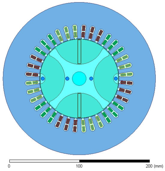
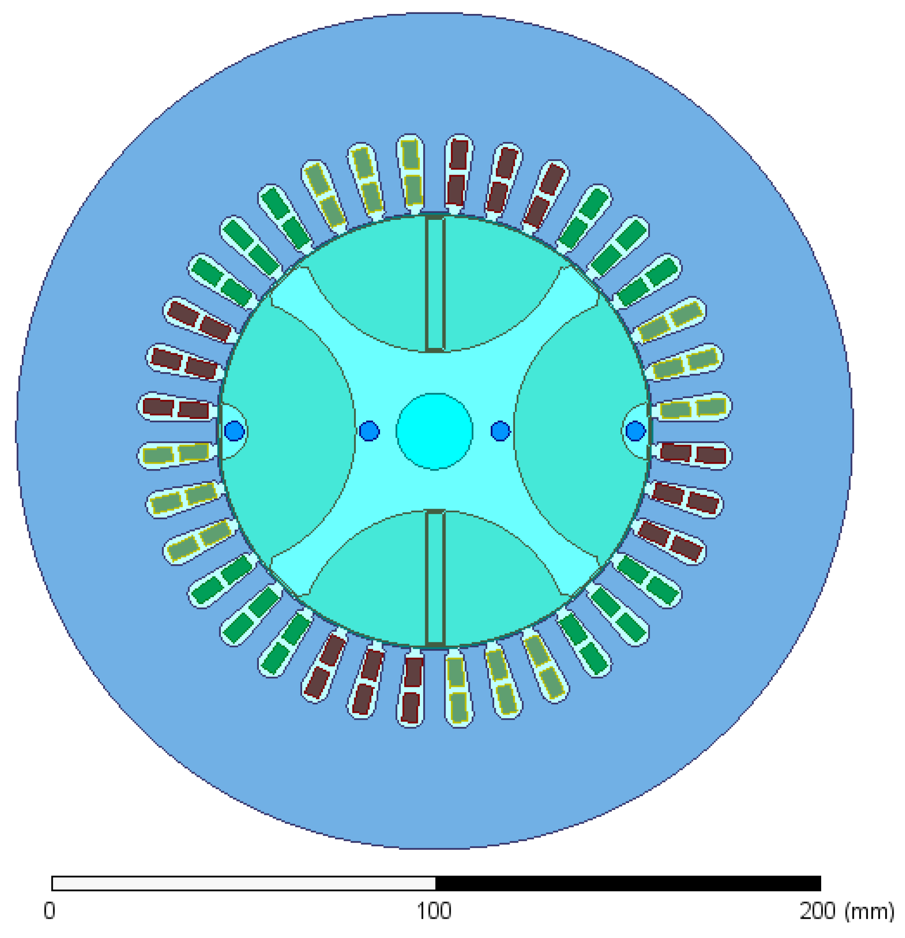
Figure 1 shows the investigated HEPMa-SynRM cross-section [1,2]. The slotted stator carries the three-phase winding; the hybrid rotor combines flux barriers, magnetic bridges, permanent magnets, and controllable DC excitation. These elements yield the two stator-current coordinates and the additional field-current coordinate used below. Their nonlinear finite-element data enter the controller simulation through the co-energy surrogate of Section 2.3.

Figure 1. Two-dimensional finite-element cross-section of the investigated HEPMa-SynRM. The outer slotted stator contains the three-phase winding; the rotor combines flux barriers, magnetic bridges, permanent magnets, and the DC-excitation winding. The scale bar is in millimeters. Colors distinguish finite-element regions and stator phase-winding groups; they do not represent a quantitative magnetic-field scale.

The study concerns the electrical current-control subsystem. Mechanical speed is prescribed and measured; torque control, speed control, current allocation, and load mechanics are outside the model. To keep the notation close to an engineering block diagram, i denotes current, u denotes voltage, and ${\omega }_e$ denotes measured electrical speed. The plant current and the voltage vector used by the controller are

$$i={\left[\begin{array}{ccc}{i}_d& i_q& i_{\mathrm{DC}}\end{array}\right]}^{\top },u_n={\left[\begin{array}{ccc}{u}_d& u_q& u_{\mathrm{DC},n}\end{array}\right]}^{\top },u_{\mathrm{DC},n}={\displaystyle \frac{2}{3}}{u}_{\mathrm{DC}}.$$

(1)

The controller state uses field current in amperes. The magnetic map uses field ampere-turns, $F_{\mathrm{DC}}=N_{\mathrm{DC}}{i}_{\mathrm{DC}}$, with $N_{\mathrm{DC}}=140$. Physical field-voltage limits are always evaluated using $u_{\mathrm{DC}}=1.5u_{\mathrm{DC},n}$. Table 1 summarizes the machine constants and electrical limits.

Table 1. Machine constants and electrical limits used in the simulations. The unit $\mathsf{\Omega }$ denotes ohms.

Quantity	Value	Origin or Status
Pole pairs p	2	magnetic model
Stator resistance $R_s$	$1.26851\mathsf{\Omega }$	phase resistance
Field resistance $R_{\mathrm{DC}}$	$6.74736\mathsf{\Omega }$	stranded-loss estimate
Map stator-current radius	$16.97056\mathrm{A}$	surrogate domain
Controller stator-current radius	$16.0\mathrm{A}$	simulation constraint
Nominal field-current limit	$7.14286\mathrm{A}$	map boundary
DC-link voltage	$565.685\mathrm{V}$	adopted datum
Stator-voltage magnitude limit	$326.599\mathrm{V}$	$V_{\mathrm{dc}}/\sqrt{3}$
Field-voltage magnitude limit	$160\mathrm{V}$	simulation constraint

2.2. Constant-Parameter Forward Model

The reciprocal constant-parameter flux model is

$$\begin{array}{cc}\hfill {\psi }_d& ={\psi }_{\mathrm{PM}}+L_d{i}_d+M_{\mathrm{DC}}{i}_{\mathrm{DC}},\hfill \\ \hfill {\psi }_q& =L_q{i}_q,\hfill \\ \hfill {\psi }_{\mathrm{DC},n}& ={\psi }_{\mathrm{DC},0,n}+M_{\mathrm{DC}}{i}_d+L_{\mathrm{DC}}{i}_{\mathrm{DC}},\hfill \end{array}$$

(2)

where ${\psi }_{\mathrm{DC},n}=(2/3)N_{\mathrm{DC}}{\psi }_{\mathrm{DC}}$ and $R_{\mathrm{DC},n}=(2/3)R_{\mathrm{DC}}$. This normalization gives the same mutual inductance in both coupled flux equations. With electrical speed ${\omega }_e$,

$$\begin{array}{cc}\hfill u_d& =R_s{i}_d+{\dot{\psi }}_d-{\omega }_e{\psi }_q,\hfill \\ \hfill u_q& =R_s{i}_q+{\dot{\psi }}_q+{\omega }_e{\psi }_d,\hfill \\ \hfill u_{\mathrm{DC},n}& =R_{\mathrm{DC},n}{i}_{\mathrm{DC}}+{\dot{\psi }}_{\mathrm{DC},n}.\hfill \end{array}$$

(3)

Let $\Delta =L_d{L}_{\mathrm{DC}}-M_{\mathrm{DC}}^2>0$. Inversion of the coupled d–field inductance block gives

$$\dot{i}=f_0(i,{\omega }_e)+G_0{u}_n,{\omega }_e=p{n}_m{\displaystyle \frac{2\pi }{60}},$$

(4)

with

$$G_0=\left[\begin{array}{ccc}{L}_{\mathrm{DC}}/\Delta & 0& -M_{\mathrm{DC}}/\Delta \\ 0& 1/L_q& 0\\ -M_{\mathrm{DC}}/\Delta & 0& L_d/\Delta \end{array}\right].$$

(5)

The measured speed ${\omega }_e$ is the only scheduling variable. The explicit drift vector and the fitted parameter values are given in Supplementary Section S1.

2.3. Energy-Consistent Chebyshev Surrogate

The finite-element solution provides flux linkages at 437 sampled current points. A controller simulation needs the flux at every integration step and, more importantly, the slope of flux with respect to current. That slope is the differential-inductance matrix. Fitting the three flux maps independently could give inconsistent cross-couplings, so all flux components were obtained from one fitted magnetic co-energy function.

The engineering meaning of the construction is summarized by

$${\lambda }_c\left(i\right)={\left[\begin{array}{ccc}(3/2){\psi }_d& (3/2){\psi }_q& N_{\mathrm{DC}}{\psi }_{\mathrm{DC}}\end{array}\right]}^{\top }={\nabla }_i{\widehat{W}}_c\left(i\right),L_{\Delta }\left(i\right)={\displaystyle \frac{2}{3}}{\displaystyle \frac{\partial {\lambda }_c}{\partial i}}={\displaystyle \frac{2}{3}}{\nabla }_i^2{\widehat{W}}_c\left(i\right).$$

(6)

Here ${\lambda }_c$ is the energy-scaled flux vector. The controller uses ${\psi }_n=(2/3){\lambda }_c$, consistently with the normalized voltage $u_n$; therefore $L_{\Delta }=\partial {\psi }_n/\partial i$ is the $3\times 3$ differential-inductance matrix in controller coordinates. Because $L_{\Delta }$ is a scaled Hessian, its stator–field cross-couplings are reciprocal by construction. The factors $3/2$ and $N_{\mathrm{DC}}$ only convert between the amplitude-invariant $dq$ variables, the field ampere-turn coordinate, and the physical field current. Their full derivation is retained in Supplementary Section S2.

Before fitting, $i_d$, $i_q$, and field magnetomotive force $F_{\mathrm{DC}}=N_{\mathrm{DC}}{i}_{\mathrm{DC}}$ were scaled to the interval $[-1,1]$. The fitted domain was

$$i_d^2+i_q^2\le {\left(16.97056\mathrm{A}\right)}^2,\left|F_{\mathrm{DC}}\right|\le 1000\mathrm{A}·\mathrm{turns}.$$

(7)

The co-energy was represented using first-kind Chebyshev polynomials,

$${\widehat{W}}_c\left(\xi \right)=\sum _{\alpha \in {\mathcal{A}}_6}{c}_{\alpha }{T}_{{\alpha }_d}\left({\xi }_d\right)T_{{\alpha }_q}\left({\xi }_q\right)T_{{\alpha }_f}\left({\xi }_f\right).$$

(8)

The index set ${\mathcal{A}}_6$ contains 49 nonconstant terms of total degree at most six. Only even powers in the q-axis coordinate were retained, matching the observed machine symmetry. Chebyshev polynomials provide a well-scaled basis on a bounded interval [23,24]; the physical consistency comes from differentiating one co-energy function, not from the polynomial family itself.

All three flux components were fitted simultaneously. Each component residual was divided by its measured span, and degree-weighted ridge regularization with coefficient ${10}^{-2}$ limited coefficient growth [25]. Degree and ridge coefficient were selected using blocked cross-validation over field-current layers, stator-current radii, and stator-current angles. Thus, neighboring points from one magnetic trajectory could not be split casually between the fit and validation blocks.

The flux-component entries in Table 2 summarize the blocked predictions by output. The combined score is formed in a different order: a joint normalized flux RMS is first computed within each blocking protocol and the three protocol scores are then averaged, as defined in Equations (S74) and (S75). RMS formation and averaging do not commute, so the combined score is not the RMS of the three displayed flux NRMSE values.

Table 2. Output-wise blocked-validation errors for the selected co-energy surrogate.

Output	RMSE	Normalized RMSE
${\psi }_d$	$0.010879\mathrm{Wb}$	0.016461
${\psi }_q$	$0.005222\mathrm{Wb}$	0.017324
${\psi }_{\mathrm{DC}}$	$8.477\times {10}^{-5}\mathrm{Wb}$	0.016571
Torque	$0.135419\mathrm{N}·\mathrm{m}$	0.001625

The combined blocked-cross-validation score was 0.017555, or approximately 1.76% of the measured flux spans. Torque was not fitted directly; as an independent physical check, it was reconstructed from the predicted d- and q-axis fluxes and had an RMSE of $0.135419\mathrm{N}·\mathrm{m}$ over an $83.343\mathrm{N}·\mathrm{m}$ measured span. The normalized co-energy Hessian was positive semidefinite at all 9809 audit points, with a minimum sampled eigenvalue of 0.862151. This is a dense numerical audit of the mapped domain, not a global proof between the sample points.

The complete differential-inductance plot is given in Supplementary Figure S1.

Synthesis rejected extrapolation beyond Equation (7). During boundary localization, diagnostic trajectories were allowed to cross the map boundary so that the terminating constraint could be identified; trajectories outside the domain were rejected, and a map-ratio halo of 1.02 was used only as an additional diagnostic flag. Such rejected trajectories do not extend the surrogate’s validated domain. The surrogate supplied the nonlinear plant used in synthesis and verification, whereas the two internal forward models retained the constant-parameter approximation. This deliberately holds the model hierarchy fixed while feedback placement is varied. ${\mathcal{M}}_1$ isolates the input map and ${\mathcal{M}}_2$ adds approximate resistance and speed-emf dynamics; the outer correction must accommodate the remaining nonlinear magnetic mismatch. Replacing all levels by the same surrogate would test a different hierarchy with a different distribution of model error. The reported comparison is conditional on the retained hierarchy and does not establish its optimality.

2.4. Nonlinear Plant and Model Hierarchy

For the nonlinear plant, the voltage equation has the familiar engineering form

$$L_{\Delta }\left(i\right)\dot{i}=u_n-b(i,{\omega }_e),\dot{i}=f_{\mathrm{Ch}}(i,{\omega }_e)+G_{\mathrm{Ch}}\left(i\right)u_n,G_{\mathrm{Ch}}\left(i\right)=L_{\Delta }{\left(i\right)}^{-1},$$

(9)

where b collects winding-resistance and speed-emf terms. The detailed coordinate conversion is given in Supplementary Section S2. The three levels of the forward-model hierarchy are then  

$$\begin{array}{cc}\hfill {\mathcal{M}}_1:& {\dot{i}}_1=G_0{U}_1,\hfill \\ \hfill {\mathcal{M}}_2:& {\dot{i}}_2=f_0(i_2,{\omega }_e)+G_0{U}_2,\hfill \\ \hfill \mathcal{P}:& {\dot{i}}_p=f_{\mathrm{Ch}}(i_p,{\omega }_e)+G_{\mathrm{Ch}}\left(i_p\right)U_p.\hfill \end{array}$$

(10)

${\mathcal{M}}_1$ retains only the constant voltage-to-current map, ${\mathcal{M}}_2$ adds resistance and speed-emf terms, and $\mathcal{P}$ uses the nonlinear differential-inductance matrix from the Chebyshev model.

3. Unified Model-Following Current-Control Architectures

3.1. Signal Relations

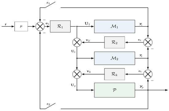
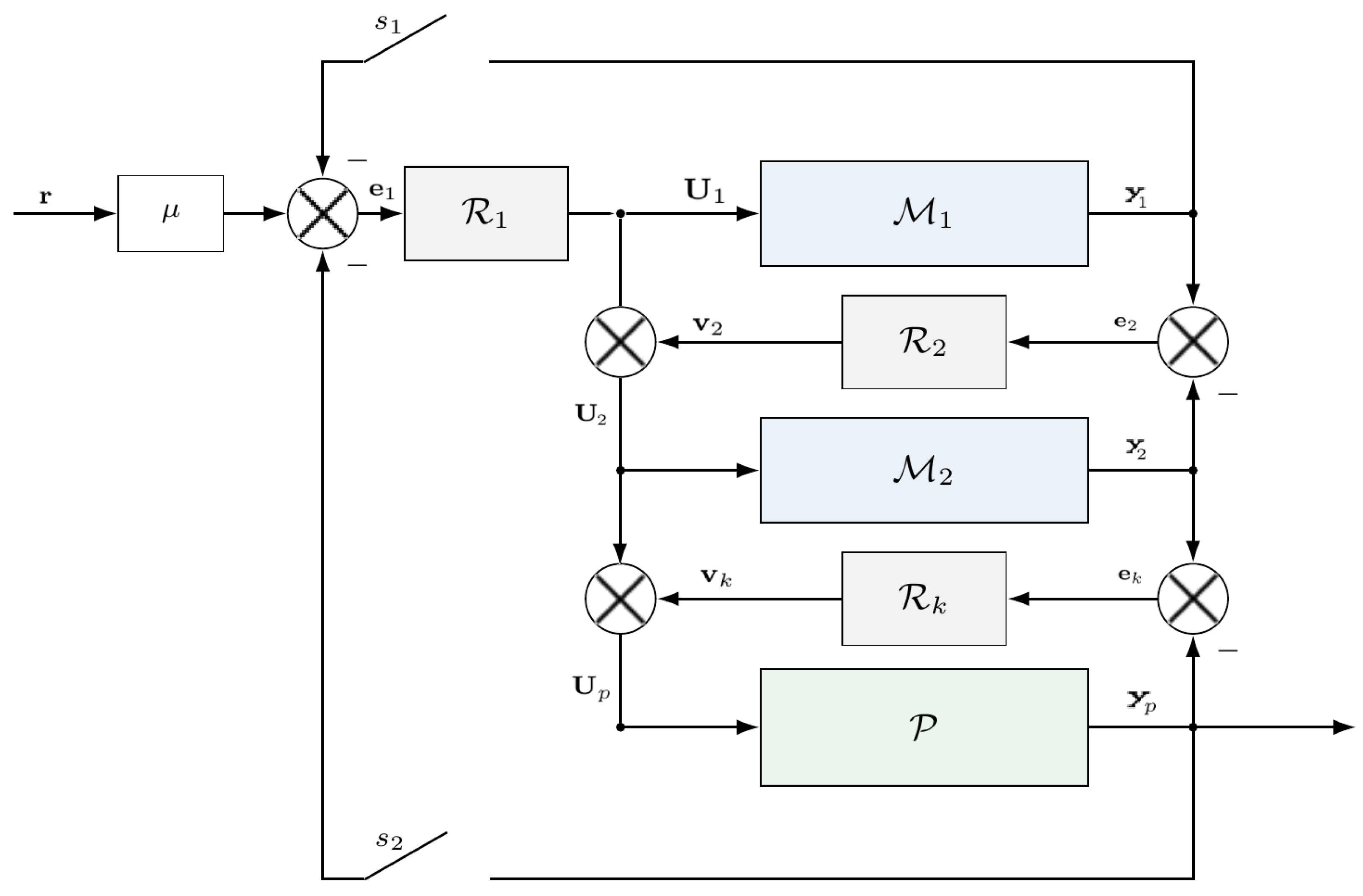
Let r be the three-current reference. The only architectural difference is the signal used by the first PI block; Table 3 lists the three alternatives. Once $e_1$ is chosen, all architectures use the same cascade relations, illustrated in Figure 2:

$$U_1={\mathcal{R}}_1\left[e_1\right],y_1={\mathcal{M}}_1\left[U_1\right],$$

(11)

$$e_2=y_1-y_2,v_2={\mathcal{R}}_2\left[e_2\right],U_2=U_1+v_2,y_2={\mathcal{M}}_2\left[U_2\right],$$

(12)

and

$$e_k=y_2-y_p,v_k={\mathcal{R}}_k\left[e_k\right],U_p=U_2+v_k,y_p=\mathcal{P}\left[U_p\right].$$

(13)

Table 3. Feedback-path settings for the three architectures.

Architecture	First-Loop Feedback	${\mathit{e}}_1$
MFCi–m	first model	$r-y_1$
MFCi–p	plant	$r-y_p$
MFCi–mp	first model and plant	$2r-y_1-y_p$

Figure 2. Unified three-loop MFC_i architecture. The notation follows Equations (11)–(13); $y_1$, $y_2$, and $y_p$ are model and plant current outputs.

Here $y_1$, $y_2$, and $y_p$ are the current outputs of the two models and the plant; $U_1$, $U_2$, and $U_p$ are cumulative voltage commands. For MFC_i–mp, the factor $2r$ preserves the intended equilibrium when model and plant feedback are used simultaneously.

3.2. PI Realization

Each correction block is a diagonal PI controller,

$${\dot{\eta }}_{\ell }=e_{\ell },{\mathcal{R}}_{\ell }\left[e_{\ell }\right]=K_{p,\ell }{e}_{\ell }+K_{i,\ell }{\eta }_{\ell },\ell \in \{1,2,k\}.$$

(14)

The three loops, two gain types, and three current channels give 18 positive gains per architecture. Synthesis, envelopes, and the original sensitivity studies test requested voltages against limits. A separate recovery study replays all fifteen originally voltage-violating cases with ideal clipping only at the plant input, using the same PI laws and no anti-windup (Supplementary Section S6.3).

4. Multiobjective Controller Synthesis

4.1. Decision Variables and Scenarios

Each architecture has 18 gains: proportional and integral gains for three current channels in each of the three loops. Rather than optimizing gains over many orders of magnitude directly, the optimizer adjusts a dimensionless multiplier $z_j$,

$$K_j=K_{j,\mathrm{seed}}{10}^{z_j},z_j\in [-b,b],j=1,\dots ,18.$$

(15)

The original synthesis used $b=1$, allowing each positive gain to vary from 0.1 to 10 times its physically scaled seed value. A second campaign used $b=1.5$, or approximately 0.03162–31.622 times the same seed values. Each domain was applied to all three architectures with the same three random seeds, solver budgets, objectives, feasibility tolerances, electrical limits, plant and internal models, and scenario/integration settings. The wider-domain campaign tests sensitivity to the finite tuning bounds; it does not establish an unconstrained optimum. Controller selection and directional-envelope verification reported below use the original-domain controllers.

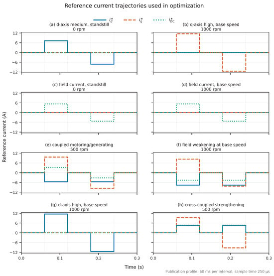
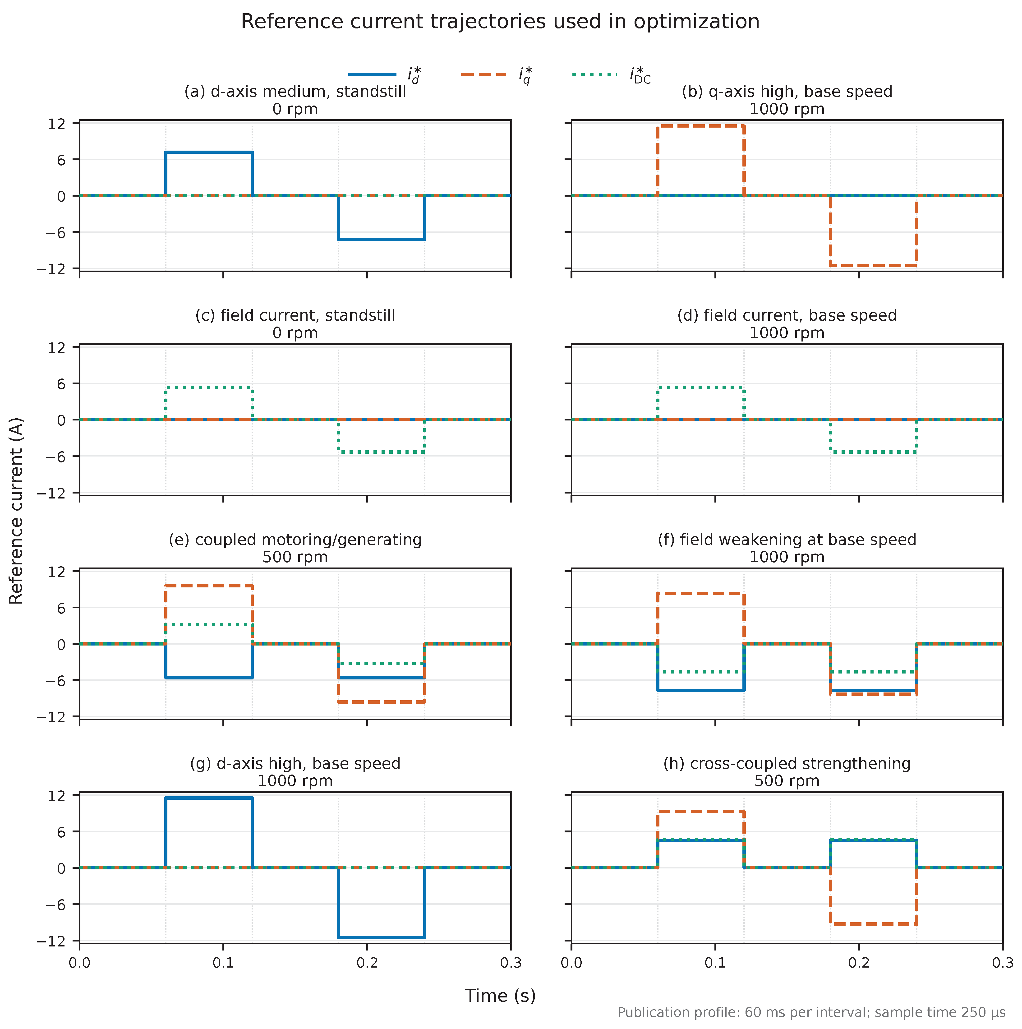
Eight equally weighted reference scenarios were used. Each scenario contains five zero-order-held intervals of $60\mathrm{ms}$, integrated by fixed-step RK4 with a 250 $\mathsf{\mu }$s step. The set contains bipolar single-axis, coupled motoring/generating, field-weakening, and field-strengthening trajectories at 0, 500, and 1000 rpm. Figure 3 gives the complete reference bank.

Figure 3. Eight current-reference trajectories used for controller synthesis: (a) medium d-axis excitation at standstill; (b) high q-axis excitation at 1000 rpm; (c) field-current excitation at standstill; (d) field-current excitation at 1000 rpm; (e) coupled motoring/generating at 500 rpm; (f) field weakening at 1000 rpm; (g) high d-axis excitation at 1000 rpm; and (h) cross-coupled field strengthening at 500 rpm. Blue solid, orange dashed, and green dotted curves denote $i_d^{★}$, $i_q^{★}$, and $i_{\mathrm{DC}}^{★}$, respectively; the superscript ★ denotes a reference command. Each panel contains five $60\mathrm{ms}$ intervals; all architectures and seeds used the same scenario bank.

4.2. Objectives and Feasibility Tests

The first objective is the mean normalized integrated absolute current error over the eight scenarios,

$$J_{\mathrm{IAE}}={\displaystyle \frac{1}{N_s}}{\displaystyle \sum _{s=1}^{N_s}}\sum _{j\in \{d,q,\mathrm{DC}\}}{\int }_0^{T_s}{\displaystyle \frac{|r_{j,s}\left(t\right)-y_{p,j,s}\left(t\right)|}{I_{j,\max }}}\mathrm{d}t.$$

(16)

The second objective is the largest fraction of either available stator or field voltage,

$$J_{\max ,u}=\underset{s,t}{\max }\left\{{\displaystyle \frac{\sqrt{u_d^2+u_q^2}}{U_{dq,\max }}},{\displaystyle \frac{|u_{\mathrm{DC}}|}{U_{\mathrm{DC},\max }}}\right\}.$$

(17)

The optimizer minimizes $(J_{\mathrm{IAE}},J_{\max ,u})$. Here $J_{\mathrm{IAE}}$ has units of seconds, $J_{\max ,u}$ is dimensionless, and $J_{\max ,u}=1$ means that at least one voltage request reaches its declared limit.

A candidate was retained as feasible when all seven implemented nonlinear checks satisfied the numerical constraint tolerance ${10}^{-5}$. Their nominal zero-tolerance requirements were: (1) the stator current to remain inside the $16\mathrm{A}$ circle; (2) the field current to remain within $7.14286\mathrm{A}$; (3) the stator voltage to remain within $326.599\mathrm{V}$; (4) the physical field voltage to remain within $160\mathrm{V}$; (5) every state to remain inside the fitted magnetic-map domain; (6) the reciprocal condition number of the differential-inductance matrix to remain at least ${10}^{-8}$; and (7) the local closed-loop linearizations on a separate equilibrium grid to satisfy the configured spectral-abscissa decay-rate test. The last test is used as a local feasibility-screening condition during synthesis.

The complete linearized state contains 18 components: the three currents of each forward model and the plant, and the nine PI integrator states. For each architecture, exact zero-error equilibria were constructed at 0 and 1000 rpm for the four normalized current vectors $(0,0,0)$, $(-0.35,0.55,0)$, $(-0.45,0.55,-0.60)$, and $(0.20,0.55,0.60)$, scaled by $(16,16,1000/140)$ A. Reference currents and speed were held fixed at each equilibrium; this test does not linearize along the changing synthesis trajectories. The Jacobian was computed by central differences with increments $h_j={10}^{-6}(1+|x_{\mathrm{cl},j}\left|\right)$ in each closed-loop state component. The nominal requirement was

$${\alpha }_{\max }:=\underset{8\mathrm{equilibria}}{\max }\max Reeig\left(A\right)\le -0.1{\mathrm{s}}^{-1},c_7={\displaystyle \frac{{\alpha }_{\max }+0.1{\mathrm{s}}^{-1}}{1000{\mathrm{s}}^{-1}}}.$$

(18)

The numerical feasibility tolerance on $c_7$ permits ${\alpha }_{\max }\le -0.09{\mathrm{s}}^{-1}$; nevertheless, the largest saved value among the 1414 original-domain controllers was $-0.118572{\mathrm{s}}^{-1}$. Thus all retained controllers also met the nominal $-0.1{\mathrm{s}}^{-1}$ threshold. The wider-domain results use the same implemented tolerance; some accepted controllers do not meet the nominal zero-tolerance threshold, as quantified in Supplementary Section S5. For the 18 original-domain selected controllers, the maximum absolute equilibrium residual was $8.04\times {10}^{-13}$ in the implemented state coordinates. This is an eight-point numerical local-stability screen based on finite-difference Jacobians. Neither their exact eigenvalues nor a nonlinear region of attraction is certified. The screen supplies no stability guarantee between operating points or for changing references and speed; the subsequent trajectory studies report finite-horizon simulation acceptance.

4.3. Solver and Controller Selection

The search used gamultiobj for population-based exploration and paretosearch for derivative-free refinement [26,27,28,29]. Each architecture was optimized independently for three fixed seeds. The hypervolume reference $[0.05\mathrm{s},1.05]$ was fixed for all architectures, seeds, and stages [30,31].

The saved configuration defines this reference as a pre-pilot performance box: 0.05 s corresponds to an aggregate normalized error of one sustained for 50 ms, while 1.05 provides a 5% margin beyond the voltage limit. Hypervolume is the dominated area inside this box divided by $0.05\times 1.05$; points outside either reference coordinate do not contribute. The custom hypervolume callbacks record progress and do not themselves stop the solvers or change the objectives. This reference therefore emphasizes the faster part of the trade-off, rather than covering every retained point.

Each run reset the Mersenne Twister with rng(seed,’twister’); the solvers used UseParallel=false. Three seeds provide a descriptive check of search variability, not evidence of global optimality. Table 4 summarizes the synthesis settings.

Table 4. Controller-synthesis settings.

Setting	Value
Software	MATLAB R2026a [32]
Decision variables	18 logarithmic PI multipliers; $[-1,1]$ originally, $[-1.5,1.5]$ in the sensitivity campaign
GA population/maximum generations	160/200
GA stall generations/Pareto fraction	30/0.5
Crossover fraction	0.8
Pareto-refinement set size	60
Maximum refinement evaluations	5000
Optimization scenarios	8 at 0, 500, and 1000 rpm
Random seeds	20260817, 20260818, 20260819
Hypervolume reference	$[0.05\mathrm{s},1.05]$

For the original-domain verification, feasible solutions were deduplicated, and nondominance was evaluated separately for each architecture. Six controllers were selected from each front before the envelope results were examined: the two objective extremes, the point closest to the normalized ideal point, and three additional points chosen to fill the largest remaining gaps along the front. This rule spreads the sample across the tracking–voltage trade-off without choosing controllers after observing their verification performance; it does not establish that six points represent the verification behavior of every nondominated controller.

4.4. Supporting Sensitivity Studies

The supporting studies hold archived controller gains fixed and change one declared part of the experiment (Table 5). Their full protocols and numerical checks are in Supplementary Sections S6–S9. The original studies use unlimited actuation; the targeted fifteen-case recovery study in Supplementary Section S6.3 additionally compares plant-voltage clipping.

Table 5. Supporting-study scope. Counts include all planned perturbed cases; matched controls/baselines are stated separately. The gain sets are from the original synthesis domain.

Study	Fixed Controllers, Changed Condition, and Case Count
Initial-current recovery	One compromise per placement; eight equilibria, three plant-current axes, $\pm 1\%$, $\pm 5\%$, $\pm 10\%$ perturbations: 432 cases and 24 equilibrium controls; 76 s observation.
Controller selection	Twelve additional controllers per placement, sampled two per front sextile without replacement; 432 twelve-ray boundaries, with the original envelope protocol.
Field-layer refitting	Three controllers per placement; nine leave-one-layer-out co-energy refits: 972 fixed-demand trajectories and 108 nominal baselines.
Sampled delay/noise	Six controllers per placement; 7560 fixed-demand cases at 10 kHz with 0/1/2-period additional delay and 0/0.1/0.5% RMS noise, plus clean 5/20-kHz checks; nonzero noise has five paired realizations.

Recovery requires both normalized plant-current and full 18-state deviations to remain below ${10}^{-3}$ through the remaining observation. The integrator scales express their voltage contributions; the full definition is in Supplementary Equation (S93). Physical acceptance checks true currents, physical voltage requests, and the map/conditioning limits. Refit and digital tracking acceptance separately require IAE within 5% of the matched nominal baseline. The digital model uses sample-and-hold, an explicit delay queue, stationary 1-kHz AR(1) measurement noise, exact affine internal-state updates, and 25 $\mathsf{\mu }$s RK4 plant integration after native pilot checks. The primary digital comparison preserves the archived baseline quadrature; an alternative piecewise-reference calculation is reported to expose threshold sensitivity. Noise parameters and update rates are benchmark assumptions, and counts are descriptive rather than failure probabilities.

5. Directional Reference-Envelope Verification

5.1. Ray Definition and Validation Set

For controller c and validation direction j, every current-reference knot is multiplied by one demand factor,

$$r_j(t;\lambda )=\lambda r_j^0\left(t\right),\lambda \in [0.2,2.0].$$

(19)

Here $\lambda$ is simply a dimensionless current-demand multiplier: $\lambda =0.8$ requests 80% of the base trajectory, $\lambda =1$ reproduces it, and $\lambda =1.2$ requests 120%. The same factor is applied to $i_d^{★}$, $i_q^{★}$, and $i_{\mathrm{DC}}^{★}$, so their signs and proportions do not change. Speed, timing, controller gains, voltage limits, and plant parameters remain fixed.

Changing $\lambda$ therefore moves the command along one fixed ray in three-dimensional current-reference space. It does not directly scale voltage or torque. The voltage is the closed-loop request required to follow the scaled current trajectory, and torque changes through the nonlinear flux map. Although electrical speed is fixed within a scenario, the speed-emf terms also depend on current-dependent flux. Neither voltage nor torque is therefore expected to vary exactly in proportion to $\lambda$.

For each controller and direction, the search reports the largest passing value ${\lambda }^{\mathrm{pass}}$. A value of 0.9 means that only 90% of the base trajectory passed; a value greater than one indicates margin beyond the base trajectory. The result is a simulated closed-loop reference envelope on the Chebyshev surrogate, not a machine capability envelope or invariant stability region.

The validation set contains the eight synthesis directions and four additional directions: medium q-axis excitation at 250 rpm, high q-axis excitation at 750 rpm, a mixed-sign cross-saturation trajectory at 1000 rpm, and a near-domain combined trajectory at 500 rpm. Validation used five $80\mathrm{ms}$ intervals and a 100 $\mathsf{\mu }$s RK4 step. Eight reference definitions overlap with synthesis, but their timing and integration protocol differ.

The added directions systematically probe two intermediate speeds, changes in the sign of stator–field interaction, and simultaneous excitation near the current bounds. They are stress-test directions, not samples from a measured duty cycle. With current fractions scaled by $(16,16,1000/140)$ A, R9 and R10 use bipolar targets $(0,0.50,0)$ and $(0,0.78,0)$; R11 uses $(0.50,0.45,-0.75)$ and $(-0.50,0.45,0.75)$; R12 uses $(-0.55,0.65,0.85)$ and $(-0.55,-0.65,-0.85)$. Each target pair is separated and bracketed by zero-current intervals, giving the five-knot sequence $(0,a,0,b,0)$.

5.2. Boundary Search and Acceptance Rule

The scale was searched over $\lambda \in [0.2,2.0]$. The algorithm advanced in increments of 0.05 and bisected the first pass–fail bracket until its width was at most 0.01. The largest final width was 0.00625. Analytical command bounds were tested before simulation; trajectory current, voltage, map, conditioning, and tracking criteria were then evaluated in a fixed order.

Tracking quality was checked using the amplitude-normalized error ratio

$$E_{\mathrm{rel}}\left(\lambda \right)={\displaystyle \frac{J_{\mathrm{IAE}}\left(\lambda \right)/\lambda }{J_{\mathrm{IAE}}\left(1\right)}}\le 1.05.$$

(20)

Thus a scaled trajectory was rejected when its tracking error per unit demand exceeded the base-trajectory value by more than 5%. Three interior points below the detected boundary were also checked for isolated non-monotone failures. This diagnostic detects pockets on the sampled grid but does not prove monotonic feasibility between samples. Because Equation (20) normalizes by demand, fixed absolute error floors receive greater relative weight at small $\lambda$; failure of this tracking criterion is not, by itself, evidence of closed-loop instability. The verification settings are summarized in Table 6.

Table 6. Directional-envelope settings.

Setting	Value
Candidates	Original sample: 18; stratified sample: 36
Rays per candidate	12
Boundaries	Original: 216; additional stratified: 432
Scale interval/march	$[0.2,2.0]$/0.05
$\lambda =1$	Nominal current-reference trajectory
Quantities not scaled by $\lambda$	Speed, timing, gains, limits, and plant parameters
Final bracket tolerance	0.01
IAE degradation threshold	1.05
Map diagnostic halo	1.02
Validation step/dwell	100 $\mathsf{\mu }$s/$80\mathrm{ms}$

5.3. Boundary Classes and Summary Measures

Each boundary was assigned to a physical or numerical cause. The worst-ray scale is simply the smallest passed demand over all 12 directions,

$${\lambda }_{\mathrm{worst},c}=\underset{j}{\min }{\lambda }_{c,j}^{\mathrm{pass}}.$$

(21)

The capability fraction compares the achieved boundary with the largest analytically admissible current command in the same direction,

$${\lambda }_{\mathrm{geo},j}=\min ({\lambda }_{I_s,j},{\lambda }_{I_f,j}),C_{c,j}={\displaystyle \frac{{\lambda }_{c,j}^{\mathrm{pass}}}{{\lambda }_{\mathrm{geo},j}}}.$$

(22)

Reference-limited rays are excluded from the candidate median of $C_{c,j}$. If a ray passes throughout the investigated interval and reaches the numerical cap $\lambda =2$, its reported value is right-censored: it establishes only ${\lambda }_{c,j}^{\mathrm{pass}}\ge 2$, not a located pass–fail boundary. The finite-protocol value 2 is retained in the reported medians of $C_{c,j}$, so C should be read as coverage of the declared search interval rather than an uncensored estimate of the attainable boundary.

6. Results

The original-domain synthesis and its verification are reported first and in the envelope subsections below. Section 6.3 presents the separate nine-run wider-domain synthesis campaign; it does not replace the controllers used in the existing verification.

6.1. Original-Domain Optimization Convergence and Pareto Sets

All nine original-domain runs completed. Pareto refinement increased final hypervolume in every run, by an architecture mean of 4.18%, 6.98%, and 4.73% for m, p, and mp. Supplementary Figure S2 gives evaluation-based convergence; Supplementary Table S8 reports the offline search work.

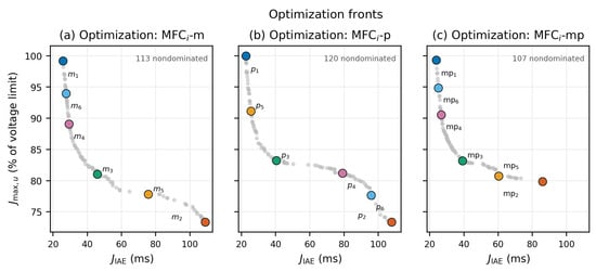
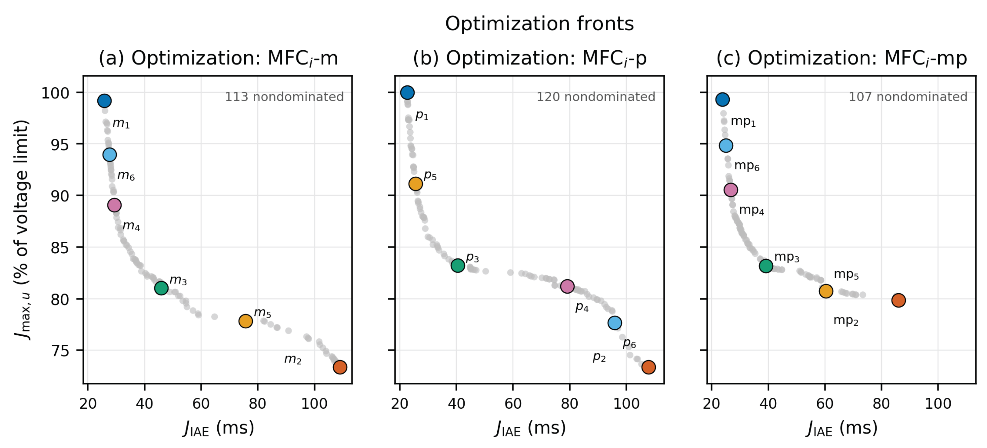
Deduplication produced 1414 optimizer-feasible controllers, summarized in Table 7. Architecture-local nondominated filtering retained 113 MFC_i–m, 120 MFC_i–p, and 107 MFC_i–mp controllers. Figure 4 shows the complete fronts and the preselected controllers.

Table 7. Original-domain optimizer-feasible pools and selected controllers.

Architecture	Feasible Pool	Nondominated	Selected
MFCi–m	469	113	6
MFCi–p	470	120	6
MFCi–mp	475	107	6
Total	1414	340	18

Figure 4. Original-domain architecture-local Pareto fronts in the synthesis objective plane: (a) MFC_i–m; (b) MFC_i–p; and (c) MFC_i–mp. Gray points show nondominated controllers pooled across three seeds. Larger colored markers identify the six preselected controllers: blue (1), minimum IAE; orange (2), minimum voltage; green (3), normalized-ideal compromise; and purple (4), yellow (5), and light blue (6), three front-spread selections. Lower coordinates are preferable on both axes. The plotted $J_{\mathrm{IAE}}$ is expressed in milliseconds; the plotted voltage objective is $100J_{\max ,u}$, expressed as a percentage of the physical voltage limit, so 100% corresponds to $J_{\max ,u}=1$. Selection precedes envelope verification.

6.2. Active Voltage Limits and Synthesis Diagnostics

For 15 of the 18 selected controllers, the synthesis voltage maximum occurred on the high-d-axis, 1000-rpm direction R7. The exceptions were ${\mathrm{p}}_1$ and ${\mathrm{p}}_2$ on high-q R2, and ${\mathrm{mp}}_4$ on field-weakening R6. Stator voltage set the maximum in 17 cases and field voltage in the remaining case (Supplementary Table S7). Hypervolume preferences also depend on the reference box: the original-domain ordering is p–mp–m at $(0.05\mathrm{s},1.05)$ and m–p–mp at $(0.12\mathrm{s},1.05)$. These post-synthesis probes and the offline evaluation counts are retained in Supplementary Section S4.

6.3. Sensitivity to the Gain Domain

All nine wider-domain runs completed with the matched publication settings. They retained 1402 feasible controllers: 472 m, 451 p, and 479 mp. Pooling the three seeds and applying architecture-local nondominated filtering gave 123, 86, and 110 front points, respectively (Table 8). These counts describe retained candidates; the larger progress-monitor archive is treated separately in Supplementary Section S5.

Table 8. Gain-domain sensitivity of retained candidate pools and pooled fronts. The two normalized hypervolumes use common references $(0.05\mathrm{s},1.05)$ and $(0.12\mathrm{s},1.05)$, respectively. Each row pools three independent runs within one domain; wider-domain rows do not include original-domain candidates.

Arch.	Logarithmic Domain	Feasible	Front	HV0.05	HV0.12
m	$[-1,1]$	469	113	0.092369	0.194574
m	$[-1.5,1.5]$	472	123	0.109266	0.257321
p	$[-1,1]$	470	120	0.100171	0.186135
p	$[-1.5,1.5]$	451	86	0.105560	0.202767
mp	$[-1,1]$	475	107	0.096517	0.176789
mp	$[-1.5,1.5]$	479	110	0.105890	0.208603

At the primary reference, the wider-domain pooled hypervolumes increased by 18.3% for m, 5.4% for p, and 9.7% for mp relative to their original-domain values. The ordering changed from p–mp–m to m–mp–p. The wider-domain ordering is also m–mp–p at the second reference, although the p–mp separation is small in the primary box. The second reference includes every original front point, but only 105/123 wider m and 103/110 wider mp points; it still includes all 86 wider p points. Neither reference summarizes the entire wider trade-off.

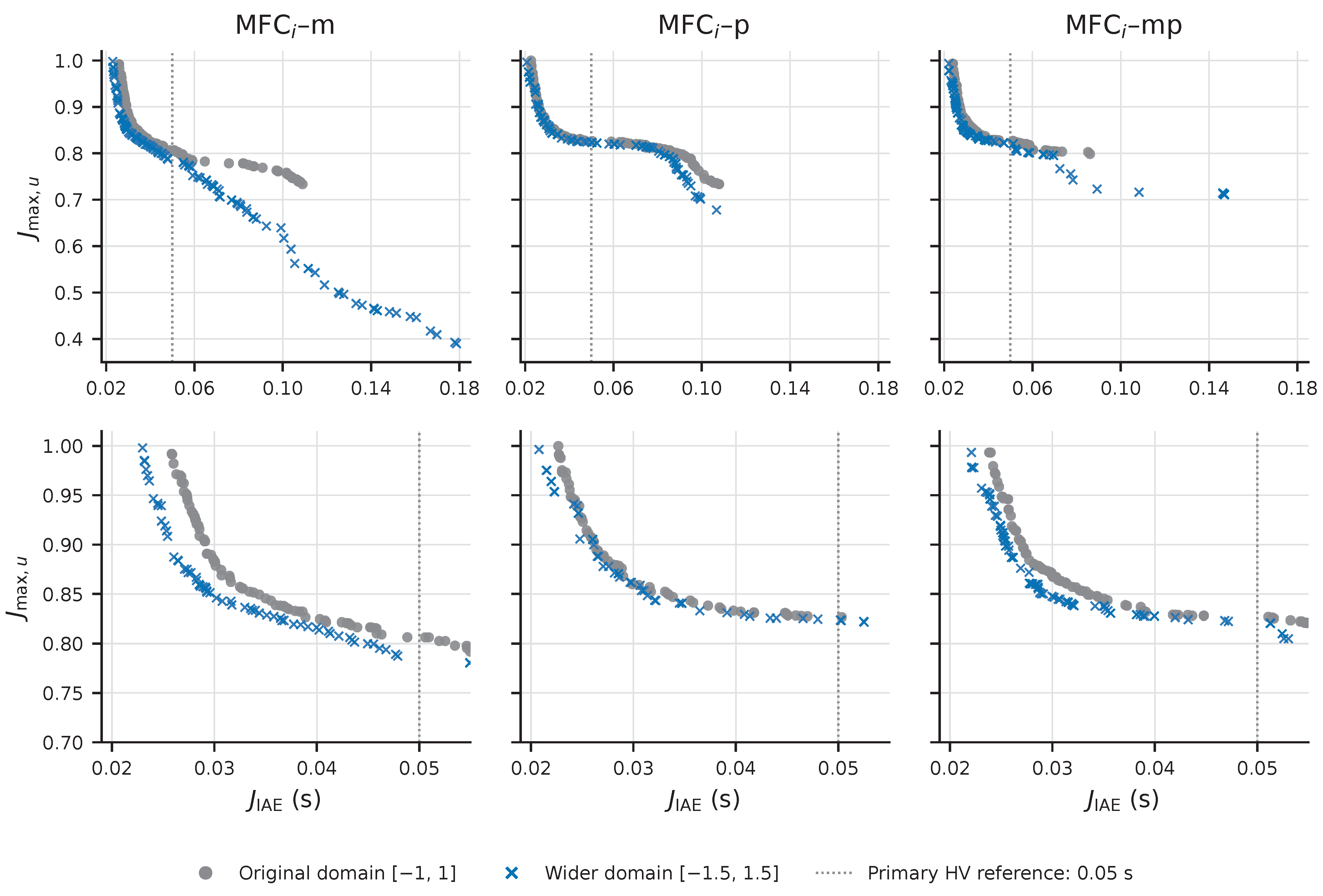
Figure 5 shows why the hypervolume result does not identify a universally preferable placement. The lowest retained tracking errors were 0.02299, 0.02079, and 0.02210 s for m, p, and mp, with respective voltage objectives 0.99799, 0.99631, and 0.99337. Thus p still reached the lowest tracking error. At the opposite m extreme, the voltage objective fell from 0.73347 to 0.38975, while tracking error increased from 0.10897 to 0.17869 s: the extra voltage reduction carries a tracking penalty.

Figure 5. Retained architecture-local nondominated fronts pooled across three seeds in each gain domain. The upper row shows the complete objective range; the lower row enlarges the faster-tracking region. The dotted line marks $J_{\mathrm{IAE}}=0.05$ s, the tracking coordinate of the primary hypervolume reference. Both axes are minimized; $J_{\max ,u}$ is dimensionless and unity reaches a physical voltage limit. Curves are separate domain-specific retained fronts, without interpolation-based performance estimates. The wider-domain controllers have not undergone directional-envelope verification.

Table 9 translates the gain-domain effect into tracking at the same voltage allowance. For m, the reductions are 15.9%, 11.0%, and 12.1% at budgets 0.80, 0.90, and 0.95, respectively. Budget 0.80 bounds both stator magnitude and physical field-voltage magnitude by 261.28 and 128.00 V. The p wider-only pool is slightly worse at 0.95, consistent with some original p points surviving on the combined front. At 0.80 m has the smallest retained IAE in both domains, whereas at 0.90 and 0.95 the wider-only mp pool has the smallest value. Thus the p tracking extreme near the full voltage limit is not a preference at every voltage budget. Candidate identities and the extraction rule are retained in the source package and Supplementary Section S5.

Table 9. Best retained tracking-error integral at common voltage budgets, in ms: original → wider gain domain. Each entry minimizes the saved $J_{\mathrm{IAE}}$ among controllers with $J_{\max ,u}\le b$; no interpolation or retuning is used. These are synthesis objectives, not settling times.

Budget b (Dimensionless)	m	p	mp
0.80	$53.49\to 44.96$	$89.57\to 81.41$	$86.04\to 64.79$
0.90	$29.27\to 26.04$	$26.39\to 26.13$	$27.13\to 25.43$
0.95	$27.34\to 24.04$	$23.89\to 24.17$	$25.06\to 23.88$

The wider fronts dominate all original m and mp front points, but ten original p points remain nondominated when both domains are combined. Keeping both sets produces a 94-point p front with primary hypervolume 0.105631, slightly above the wider-only value 0.105560; the combined m and mp fronts are unchanged. A larger admissible domain therefore need not make a finite stochastic search recover every previously found trade-off.

Almost every wider-front controller lies outside the original gain box, and outer-bound activity remains frequent (Table S10). The campaign demonstrates sensitivity to the prescribed gain limits while leaving the optimum beyond the tested domain unresolved. Its pooled ranking is descriptive: the three individual-seed hypervolume ranges overlap, and no statistical architecture-superiority claim is made.

6.4. Directional Envelope and Selection Sensitivity

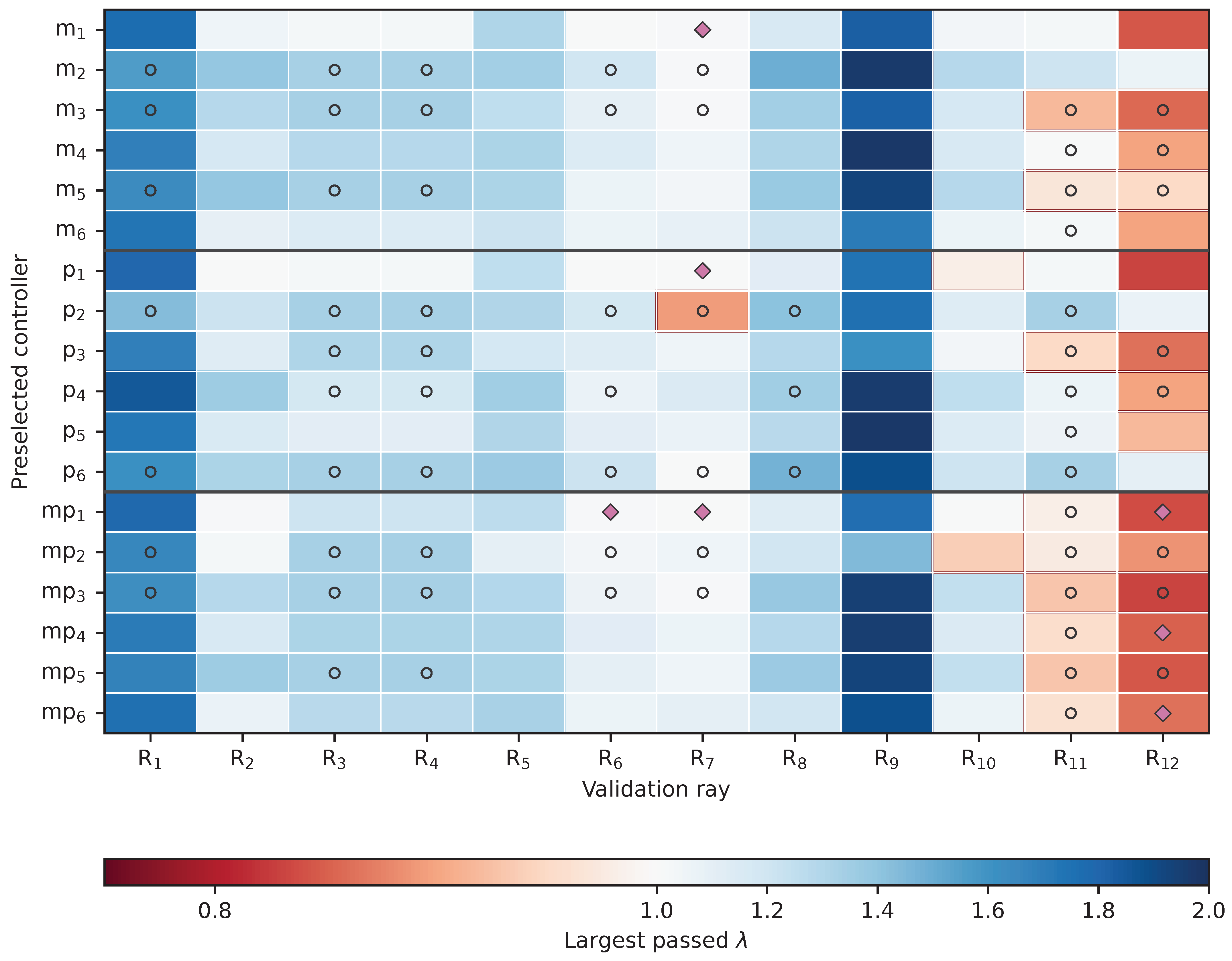
In the original six-controller sample, 189/216 base trajectories passed. The first failures were 18 field-current, eight stator-current, and one stator-voltage violations, concentrated on R11 and R12. The coincident field-current and field-map boundary matters directly for this machine. Figure 6 retains the full directional view; the boundaries are finite-search acceptance results, including censored reference-geometry limits and detected internal tracking failures.

Figure 6. Ray-resolved verification margins for the 18 controllers preselected from the architecture-specific Pareto fronts. Rows ${\mathrm{m}}_1,\dots ,{\mathrm{m}}_6$, ${\mathrm{p}}_1,\dots ,{\mathrm{p}}_6$, and ${\mathrm{mp}}_1,\dots ,{\mathrm{mp}}_6$ identify the six preselected controllers of each MFC_i architecture. Cell color denotes the largest passed demand multiplier ${\lambda }_{c,j}^{\mathrm{pass}}$ for controller c and validation ray $R_j$; $\lambda =1$ corresponds to the unscaled reference. A red cell border indicates ${\lambda }_{c,j}^{\mathrm{pass}}<1$. Open circles denote censored, reference-geometry-limited boundaries, while magenta diamonds identify detected internal non-monotone IAE-degradation pockets. No boundary in this sample is search-cap limited.

The original m/p worst-ray medians differ by less than the declared 0.01 localization tolerance; their endpoint spans overlap. The original p sample has the largest median normalized capability. The twelve additional stratified controllers per placement change this comparison (Table 10): m has the largest capability median, while p has the largest worst-ray median. The new worst-ray endpoint spans are $[0.8750,0.88125]$, $[0.89375,0.9000]$, and $[0.8500,0.85625]$ for m, p, and mp. These spans describe numerical localization, not population confidence. All searches completed, and no boundary reached the search cap.

Table 10. Envelope summaries for the original and additional stratified selections. n is controllers per placement. C is the controller-wise median capability fraction after excluding reference-limited rays. All metrics are dimensionless; medians describe these samples only. The final column counts controllers passing every base-demand ray. Full ranges and endpoint spans are in Supplementary Section S7.

Placement	Selection	n	Median ${\mathit{\lambda }}_{\mathbf{worst}}$	Median C	Base Passes	All 12
m	Original	6	0.9000	0.8045	65/72	1/6
m	Stratified	12	0.8750	0.8244	125/144	1/12
p	Original	6	0.8969	0.8529	65/72	1/6
p	Stratified	12	0.89375	0.8160	130/144	1/12
mp	Original	6	0.8469	0.8058	59/72	0/6
mp	Stratified	12	0.8500	0.7748	119/144	0/12

Only one m and one p controller in each selection pass all twelve base rays; none of the selected mp controllers does. The additional selection passes 374/432 base trajectories. These outcomes favor verifying individual gains on all required directions rather than selecting an architecture from a single aggregate median. Supplementary Section S7 retains the selection protocol, full diagnostics, and matched-demand replay.

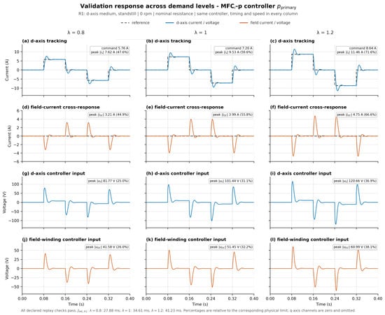
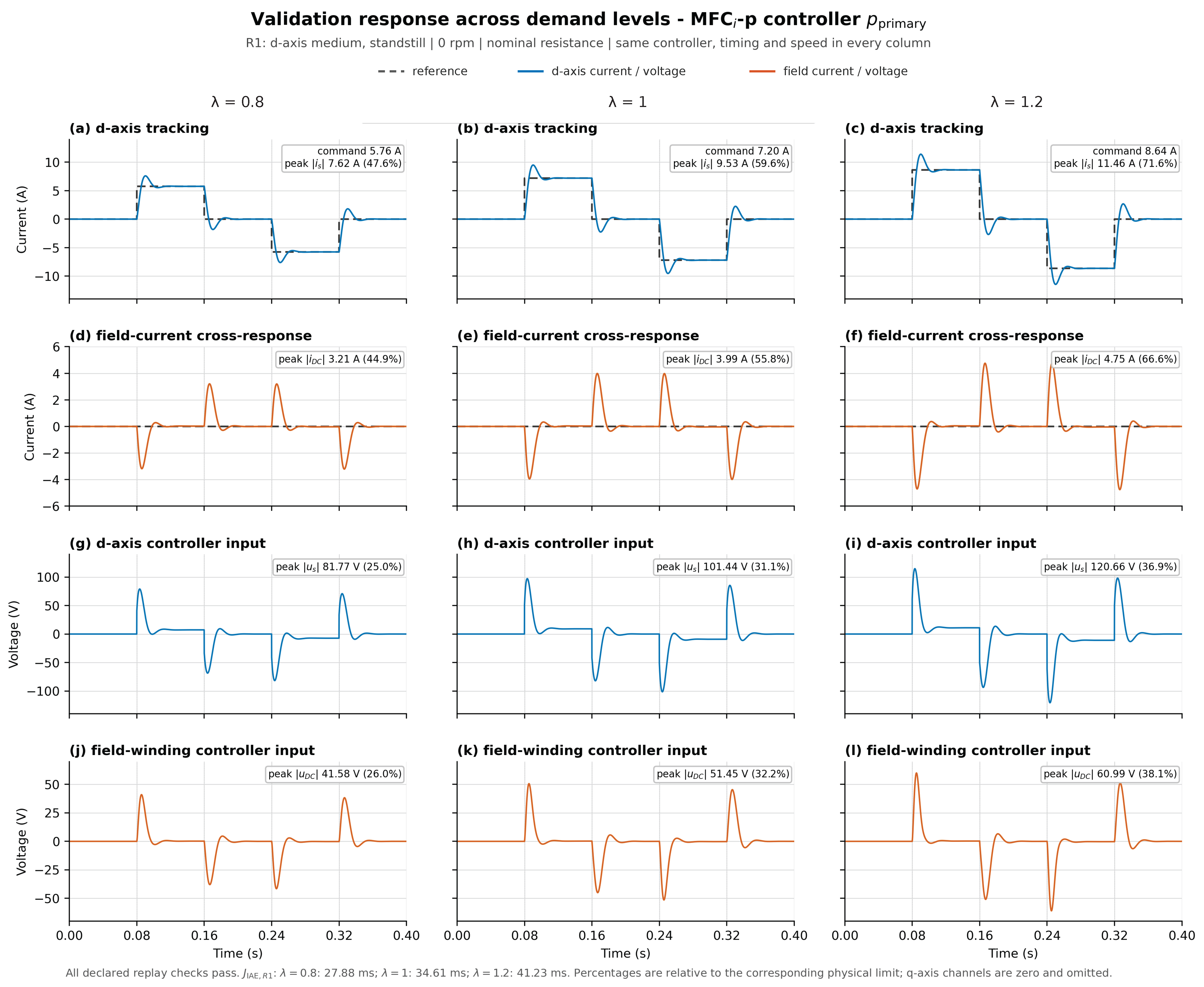
6.5. Representative Time-Domain Response

Figure 7 uses the selected p-primary controller on the R1 standstill d-axis scenario as an illustration of demand scaling. R1 separates the coupled current and voltage transients from speed-emf effects; the unchanged p controller makes the three amplitudes directly comparable. This single-controller example does not determine the architecture ranking. The three columns apply 80%, 100%, and 120% of the same nominal current command; the controller, zero-speed condition, timing, and limits are unchanged. All three simulations passed. As $\lambda$ increased from 0.8 to 1.2, $J_{\mathrm{IAE},R1}$ increased from 27.88 to 41.23 ms, peak stator voltage from 81.77 to 120.66 V, and peak field voltage from 41.58 to 60.99 V.

Figure 7. Plant currents and physical voltage requests for the p-primary controller on validation scenario R1. The left, middle, and right columns use 80%, 100%, and 120% of the nominal current-reference amplitude, respectively. The panels show: (a) d-axis current tracking at $\lambda =0.8$; (b) d-axis current tracking at $\lambda =1$; (c) d-axis current tracking at $\lambda =1.2$; (d) field-current cross-response at $\lambda =0.8$; (e) field-current cross-response at $\lambda =1$; (f) field-current cross-response at $\lambda =1.2$; (g) d-axis voltage command at $\lambda =0.8$; (h) d-axis voltage command at $\lambda =1$; (i) d-axis voltage command at $\lambda =1.2$; (j) physical field-winding voltage command at $\lambda =0.8$; (k) physical field-winding voltage command at $\lambda =1$; and (l) physical field-winding voltage command at $\lambda =1.2$. Gray dashed curves denote current references, blue solid curves denote d-axis currents or voltages, and orange solid curves denote field currents or voltages. Speed, controller gains, timing, and limits are unchanged; voltage is a simulated response and is not scaled directly. All panels use common physical-unit limits. The reported $J_{\mathrm{IAE},R1}$ is a single-scenario quantity in ms, not the mean synthesis objective. R1 at standstill isolates the coupled transient for a fixed illustrative p controller; the figure is not an architecture comparison.

6.6. Initial-Current Recovery and Voltage Feasibility

All 432 perturbed cases of the three original compromise controllers recovered by the joint current/full-state criterion; all 24 equilibrium controls passed. Sampled electrical feasibility was 144/144 for m, 143/144 for p, and 130/144 for mp. Median return times were 23.10, 22.95, and 16.84 ms, respectively; the shortest median therefore does not imply feasible actuation. The fifteen violations were stator-voltage requests after initial q-current perturbations. The largest, 564.28 V for mp, was 1.728 times the available voltage; the sole p violation reached 392.02 V. No other current or field-voltage limit was exceeded. Supplementary Section S6 gives the operating points, phase projections, and numerical checks for the original unsaturated study.

A targeted follow-up replays all fifteen voltage-violating initial conditions with unlimited and clipped plant voltage, each at base and tighter numerical tolerances: sixty completed integrations. Gains, internal models, reference conditions, the 76 s horizon, and the joint current/full-state recovery criterion are unchanged. The limiter applies a 326.60-V stator circle and a signed 160-V physical field bound only to the plant; no anti-windup is added.

All fifteen clipped cases recover and pass the sampled current, applied-voltage, map, and conditioning limits. For the sole p case, $t_r$ changes from 23.1 to 22.9 ms. Across the fourteen mp cases, median return time changes from 61.50 to 62.65 ms; the median paired increase is 0.95 ms. The largest increase occurs in the prespecified worst-voltage case, from 64.2 to 109.9 ms (45.7 ms, or 71.2%). Recovery-current IAE increases by 7.1% for p and by 0.004–32.5% for mp, with a 0.62% median paired increase for mp. All thirty base/tight repeat checks pass. Supplementary Section S6.3 gives the limiter, case-level results, numerical comparisons, and the two prespecified trajectory examples. This closes the missing clipping comparison for the fifteen observed violations under the ideal average-voltage model. The unequal targeted sets (one p, fourteen mp, and no m violation) do not rank architectures or certify a saturated region of attraction.

6.7. Magnetic Refit and Sampled Implementation Sensitivity

Table 11 summarizes tracking sensitivity to nine field-layer refits. Every alternate-plant case completed and met the 5% tracking-change criterion; changes ranged from $-0.1931\%$ to $+0.0629\%$. Four p voltage classifications lie only 0.0010–0.0396% above the limit and remain unresolved under targeted step refinement. They are not evidence of a robust feasibility ordering. Full refit diagnostics are in Supplementary Section S8.

Table 11. Field-layer refit summary: three fixed controllers per placement, 324 alternate-plant cases each. Maximum absolute IAE change is relative to the matching nominal trajectory, using the archived quadrature.

Measure	m	p	mp
Maximum absolute IAE change (%)	0.1380	0.1595	0.1931
Cases within 5% tracking change	324/324	324/324	324/324

The 7560 sampled-controller cases give the selected m set the highest aggregate physical acceptance (1890/2520, compared with 1799/2520 for p and 1520/2520 for mp) and combined physical/tracking acceptance (Table 12). Of the 278 map-guard terminations, 113 were p and 165 mp, all at two-period additional delay; these outcomes remain failures in the denominators. The ordering is conditional: at clean one-period delay, p has 55/72 physical passes and m 54/72, while their combined counts tie at 54/72. Changing to piecewise-reference quadrature for both trajectories changes 101 combined decisions and gives totals 1556, 1394, and 1124, preserving the aggregate ordering. Supplementary Section S9 retains every delay/noise setting, realization range, guard outcome, and quadrature diagnostic.

Table 12. Selected sampled-controller conditions and aggregate combined acceptance (physical limits plus IAE within 5% of the matched continuous baseline). Conditions use 10 kHz, additional delay d in periods, and noise RMS as a percentage of current scales. Entries are passed/total counts. The total includes 5/20-kHz clean checks. Nonzero noise has five realizations, so aggregate counts do not estimate deployment success probabilities.

d	Noise (%)	m	p	mp
0	0.0	64/72	64/72	59/72
1	0.1	265/360	250/360	207/360
2	0.0	44/72	36/72	29/72
2	0.5	114/360	99/360	50/360
All settings		1597/2520	1423/2520	1155/2520
All settings (%)		63.4	56.5	45.8

7. Discussion

7.1. Practical Placement Choice

The comparison supplies useful starting points without a universal architecture ordering. Table 13 connects each design priority to the available evidence. The p placement reaches the lowest retained IAE near the full voltage allowance in both gain domains. Under a tighter voltage budget, the retained front matters more than that extreme: m has the lowest error at budget 0.80, while the wider mp pool has the lowest value at 0.90 and 0.95. An mp candidate can therefore be useful for a particular budget even though the tested mp sets provide no consistent aggregate envelope or delay/noise benefit.

Table 13. Evidence-based starting points for placement selection under the declared model and protocols. Final selection requires candidate-level checks.

Design Priority	Starting Point and Required Check
Lowest tracking-error extreme	Include p: it gives the smallest retained IAE in both domains. Check its near-limit voltage demand and the required rays.
Tight voltage allowance	Include m at budget 0.80; compare all fronts at the actual budget. Wider mp is competitive at 0.90/0.95 in the saved pools.
Delay/noise sensitivity	Retain m candidates: the selected m set has the highest aggregate acceptance. Repeat the benchmark with the intended timing and sensor characteristics.
Every required direction passes	Verify each gain set on every required ray. Only one m and one p in each tested selection pass all twelve base rays.
Combined feedback by default	The tested mp sets give no consistent aggregate advantage. Select mp when a verified candidate improves the specified criterion.

Envelope selection must also declare the metric. Worst-ray scale measures the earliest observed directional boundary regardless of cause, whereas C measures utilization relative to the admissible current-command geometry. The stratified sample favors p for the former and m for the latter. Their medians summarize the sampled gain sets; neither substitutes for the full ray results. Physical field voltage must be converted as $u_{\mathrm{DC}}=1.5u_{\mathrm{DC},n}$ in any converter comparison.

The work extends established multi-loop MFC realizations to a common saturated three-current comparison [13,14,15,19]. The machine topology and magnetic data retain their prior attribution [1,2]. The practical guidance is specific to this PI-based realization and does not imply superiority over other current-control families [7,9].

7.2. Limits of the Evidence

The plant surrogate is shared by synthesis and verification. Broader rays, field-layer refits, and sampled-control tests provide scenario and model sensitivity evidence, not independent plant validation. The stated current and voltage bounds are simulation constraints. Mechanical dynamics, current allocation, switching, dead time, thermal drift, and anti-windup are absent. Ideal voltage clipping is tested in the fifteen-case recovery follow-up; it is not included in synthesis, envelopes, or the delay/noise study. The eight-equilibrium finite-difference screen is numerical and local; neither a regional Lyapunov certificate nor a nonlinear region of attraction is reported. Envelope and recovery conclusions are finite-horizon results for the sampled directions and perturbations.

Three synthesis seeds and persistent active gain bounds leave the unconstrained optimum unresolved. One stratified draw establishes selection sensitivity without population confidence intervals. Wider-gain controllers have not undergone envelope verification; delay/noise tests use only the original eighteen controllers. Small refit tracking changes concern the specified refit family, and the four marginal p voltage crossings remain unresolved. Digital threshold decisions depend on baseline quadrature, and finite pilot checks do not resolve every near-threshold outcome. Actual sensing, execution timing, converter dynamics, and HIL or hardware tests are needed to turn these candidate-selection guidelines into deployment recommendations.

8. Conclusions

The three MFC_i placements provide different useful trade-offs on a common saturated HEPMa-SynRM plant. The p placement achieves the lowest retained tracking-error integral in both tested gain domains. The m placement is a strong candidate when the voltage allowance is tight or the tested delay/noise sensitivity is a priority. Combined mp feedback does not establish a consistent aggregate advantage for default selection, although individual mp candidates can improve a specified voltage-budget trade-off.

These preferences depend on the design protocol. Widening the gain domain changes the primary pooled hypervolume ordering from p–mp–m to m–mp–p. For m at an 80% voltage budget, the best retained IAE falls from 53.49 to 44.96 ms, a 15.9% reduction at the same allowance. Controller selection also changes the envelope interpretation: the original p capability-median advantage does not persist in the stratified sample, which favors m for normalized capability and p for worst-ray scale. Individual gain sets must therefore be checked on every required operating direction.

The supporting studies refine this guidance. Nine field-layer refits change tracking IAE by less than 0.20% for the tested controllers. The original selected m set has the highest aggregate combined acceptance in the sampled delay/noise benchmark. All 432 initial-current perturbations recover in the unsaturated model, while fifteen request excessive stator voltage; recovery and feasible actuation must consequently be kept distinct. All fifteen violating cases also recover in the matched ideal-clipping replays without anti-windup. The largest mp return-time increase is from 64.2 to 109.9 ms.

The conclusions are simulation-based and conditional on the declared surrogate, gain bounds, controller selections, and acceptance rules. The stability evidence is an eight-point numerical local screen supplemented by finite-horizon trajectories. The completed clipping study covers the fifteen observed voltage violations. An anti-windup design, wider-gain envelope verification, and target-controller or hardware validation are not supplied.

References

- Wardach, M.; Prajzendanc, P.; Palka, R.; Cierzniewski, K.; Pstrokoński, R.; Cichowicz, M.; Pacholski, S.; Ciuruś, J.; Hao, C. Hybrid-Excited Permanent Magnet-Assisted Synchronous Reluctance Machine. Energies 2022, 15, 2997. [Google Scholar] [CrossRef] [Scilit]
- Palka, R.; Cierzniewski, K.; Wardach, M.; Prajzendanc, P. Research on Innovative Hybrid Excited Synchronous Machine. Energies 2023, 16, 6600. [Google Scholar] [CrossRef] [Scilit]
- Pothi, N.; Zhu, Z.Q.; Afinowi, I.A.A.; Lee, B.; Ren, Y. Control Strategy for Hybrid-Excited Switched-Flux Permanent Magnet Machines. IET Electr. Power Appl. 2015, 9, 612–619. [Google Scholar] [CrossRef] [Scilit]
- Jebai, A.K.; Combes, P.; Malrait, F.; Martin, P.; Rouchon, P. Energy-Based Modeling of Electric Motors. In Proceedings of the 53rd IEEE Conference on Decision and Control, Los Angeles, CA, USA, 15–17 December 2014; pp. 6009–6016. [Google Scholar] [CrossRef] [Scilit]
- Rasilo, P.; Lemesle, M.A.; Belahcen, A.; Arkkio, A.; Hinkkanen, M. Comparison of Finite-Element-Based State-Space Models for PM Synchronous Machines. IEEE Trans. Energy Convers. 2014, 29, 535–543. [Google Scholar] [CrossRef] [Scilit][Green Version]
- Carbonieri, M.; Di Leonardo, L.; Mahmoudi, A.; Tursini, M.; Bianchi, N.; Soong, W.L. Fast Flux Mapping Technique for Synchronous Reluctance Machines: Method Description and Comparison With Full FEA and Measurements. IEEE Trans. Ind. Appl. 2023, 59, 4056–4065. [Google Scholar] [CrossRef] [Scilit]
- Awan, H.A.A.; Saarakkala, S.E.; Hinkkanen, M. Flux-Linkage-Based Current Control of Saturated Synchronous Motors. IEEE Trans. Ind. Appl. 2019, 55, 4762–4769. [Google Scholar] [CrossRef] [Scilit]
- Ma, H.; Li, L.; Fan, Y.; Guo, Y.; Jin, Z.; Luo, J. A Discrete Current Controller for High Power-Density Synchronous Machines. Energies 2022, 15, 6396. [Google Scholar] [CrossRef] [Scilit]
- Zanelli, A.; Kullick, J.; Eldeeb, H.M.; Frison, G.; Hackl, C.M.; Diehl, M. Continuous Control Set Nonlinear Model Predictive Control of Reluctance Synchronous Machines. IEEE Trans. Control Syst. Technol. 2022, 30, 130–141. [Google Scholar] [CrossRef] [Scilit]
- Hou, Q.; Wang, H.; Lee, C.H.T.; Ding, S. Composite Adaptive Super-Twisting Sliding Mode Control Using Barrier Function for PM Motor Drives Toward Electric Aircraft Applications. IEEE Trans. Power Electron. 2025, 40, 16255–16264. [Google Scholar] [CrossRef] [Scilit]
- Hou, Q.; Wang, H.; Zhao, C.; Xu, S.; Zuo, Y.; Lee, C.H.T.; Ding, S. STESO-Based Quasi-Proportional-Resonant Controller for Permanent Magnet Synchronous Motor Drive System. IEEE Trans. Transp. Electrif. 2024, 10, 1596–1604. [Google Scholar] [CrossRef] [Scilit]
- Rivera, D.E.; Morari, M.; Skogestad, S. Internal Model Control: PID Controller Design. Ind. Eng. Chem. Process Des. Dev. 1986, 25, 252–265. [Google Scholar] [CrossRef] [Scilit]
- Skoczowski, S. Robust Model Following Control with Use of Plant Model. Int. J. Syst. Sci. 2001, 32, 1413–1427. [Google Scholar] [CrossRef] [Scilit]
- Osypiuk, R. Simple Robust Control Structures Based on the Model-Following Concept—A Theoretical Analysis. Int. J. Robust. Nonlinear Control 2010, 20, 1920–1929. [Google Scholar] [CrossRef] [Scilit]
- Osypiuk, R.; Finkemeyer, B.; Wahl, F.M. Multi-Loop Model-Based Control Structure for Robot Manipulators. Robotica 2005, 23, 491–499. [Google Scholar] [CrossRef] [Scilit]
- Osypiuk, R.; Finkemeyer, B.; Skoczowski, S. Simple Two Degree of Freedom Structures and Their Properties. Robotica 2006, 24, 365–372. [Google Scholar] [CrossRef] [Scilit]
- Skoczowski, S.; Domek, S.; Pietrusewicz, K.; Broel-Plater, B. A Method for Improving the Robustness of PID Control. IEEE Trans. Ind. Electron. 2005, 52, 1669–1676. [Google Scholar] [CrossRef] [Scilit]
- Osypiuk, R.; Kröger, T. A Three-Loop Model-Following Control Structure: Theory and Implementation. Int. J. Control 2010, 83, 97–104. [Google Scholar] [CrossRef] [Scilit]
- Osypiuk, R. A New Approach to Compensator Design Based on Multi-Loop Technique and Scalable Forward Model Complexity. Electronics 2021, 10, 3049. [Google Scholar] [CrossRef] [Scilit]
- Pietrusewicz, K.; Waszczuk, P.; Kubicki, M. MFC/IMC Control Algorithm for Reduction of Load Torque Disturbance in PMSM Servo Drive Systems. Appl. Sci. 2019, 9, 86. [Google Scholar] [CrossRef] [Scilit]
- Willkomm, J.; Wulff, K.; Reger, J. Quantitative Robustness Analysis of Model Following Control for Nonlinear Systems Subject to Model Uncertainties. IFAC-PapersOnLine 2021, 54, 167–172. [Google Scholar] [CrossRef] [Scilit]
- Willkomm, J.; Wulff, K.; Reger, J. Set-Point Tracking for Nonlinear Systems Subject to Uncertainties Using Model-Following Control with a High-Gain Controller. In Proceedings of the 2022 European Control Conference (ECC), London, UK, 12–15 July 2022; pp. 1617–1622. [Google Scholar] [CrossRef] [Scilit]
- Pries, J.; Burress, T. High Fidelity D-Q Modeling of Synchronous Machines Using Spectral Interpolation. In Proceedings of the 2017 IEEE Transportation Electrification Conference and Expo (ITEC), Chicago, IL, USA, 22–24 June 2017; pp. 779–785. [Google Scholar] [CrossRef] [Scilit]
- Trefethen, L.N. Approximation Theory and Approximation Practice; Society for Industrial and Applied Mathematics: Philadelphia, PA, USA, 2013. [Google Scholar]
- Hoerl, A.E.; Kennard, R.W. Ridge Regression: Biased Estimation for Nonorthogonal Problems. Technometrics 1970, 12, 55–67. [Google Scholar] [CrossRef]
- Deb, K.; Pratap, A.; Agarwal, S.; Meyarivan, T. A Fast and Elitist Multiobjective Genetic Algorithm: NSGA-II. IEEE Trans. Evol. Comput. 2002, 6, 182–197. [Google Scholar] [CrossRef] [Scilit]
- Custódio, A.L.; Madeira, J.F.A.; Vaz, A.I.F.; Vicente, L.N. Direct Multisearch for Multiobjective Optimization. SIAM J. Optim. 2011, 21, 1109–1140. [Google Scholar] [CrossRef] [Scilit]
- The MathWorks, Inc. gamultiobj: Find Pareto Front of Multiple Fitness Functions Using Genetic Algorithm. Global Optimization Toolbox Documentation for MATLAB R2026a. 2026. Available online: https://www.mathworks.com/help/releases/R2026a/gads/gamultiobj.html (accessed on 30 September 2026).
- The MathWorks, Inc. paretosearch: Find Points in Pareto Set. Global Optimization Toolbox Documentation for MATLAB R2026a. 2026. Available online: https://www.mathworks.com/help/releases/R2026a/gads/paretosearch.html (accessed on 30 September 2026).
- Zitzler, E.; Thiele, L. Multiobjective Evolutionary Algorithms: A Comparative Case Study and the Strength Pareto Approach. IEEE Trans. Evol. Comput. 1999, 3, 257–271. [Google Scholar] [CrossRef] [Scilit]
- Guerreiro, A.P.; Fonseca, C.M.; Paquete, L. The Hypervolume Indicator: Computational Problems and Algorithms. ACM Comput. Surv. 2021, 54, 1–42. [Google Scholar] [CrossRef] [Scilit]
- The MathWorks, Inc. MATLAB Release R2026a (Version 26.1); Computer Software; The MathWorks, Inc.: Natick, MA, USA, 2026; Official Release Listing; Available online: https://www.mathworks.com/support/requirements/previous-releases.html (accessed on 30 September 2026).
Disclaimer/Publisher’s Note: The statements, opinions and data contained in all publications are solely those of the individual author(s) and contributor(s) and not of MDPI and/or the editor(s). MDPI and/or the editor(s) disclaim responsibility for any injury to people or property resulting from any ideas, methods, instructions or products referred to in the content. |
© 2026 by the authors. Licensee MDPI, Basel, Switzerland. This article is an open access article distributed under the terms and conditions of the Creative Commons Attribution (CC BY) license.