


Abstract
In hot arid climates, combined cycle power plants (CCPPs) can experience reduced performance as high ambient temperature increases compressor inlet temperature and specific compression work. This study develops a steady-state energy, exergy, and exergoeconomic model of a 750 MW CCPP integrated with an ice thermal energy storage (ITES) cooling subsystem under Basra, Iraq, climatic conditions. Four configurations are evaluated: a standard plant without cooling, compressor-inlet cooling, air-cooled-condenser (ACC) inlet cooling, and simultaneous dual-point cooling of the compressor and ACC inlet air. Twelve monthly meteorological conditions are used to characterize the seasonal operating envelope, while the annual-mean condition is used for the comparative optimization. Four objective functions are evaluated through independent single-objective genetic-algorithm (GA) runs: minimization of total operating cost rate, minimization of fuel cost rate, maximization of thermal efficiency, and maximization of exergy efficiency. The reported optimization results are therefore objective-specific rather than a single Pareto multi-objective optimum. At the common total-operating-cost objective, the reported optimum gives 9.468 × 10⁻³ USD/s for Case 2, 8.993 × 10⁻³ USD/s for Case 3, and 8.993 × 10⁻³ USD/s for Case 4, compared with 9.721 × 10⁻³ USD/s for the standard case. Under the corresponding Case-3 and Case-4 total-cost runs, the thermal efficiency is 49.44%, compared with 48.86% for the standard case. Exergy analysis shows that the combustion chamber remains the dominant source of exergy destruction. The results quantify the thermodynamic and economic effects of the alternative cooling configurations within the adopted steady-state model, while the transient charge/discharge behavior of the ITES tank remains outside the present model boundary.
1. Introduction
The need to use our limited fossil fuel resources as efficiently as possible and to keep the costs of energy production as low as possible has kept the subject of the thermodynamic optimization of large-scale power generation systems in the interest. Of these, the most efficient configuration of gas-fueled electricity generation in commercial operation today is combined cycle power plants (CCPPs) consisting of a heat recovery steam generator (HRSG) between a Brayton-cycle gas turbine topping and a Rankine-cycle steam turbine bottoming cycle [1,2]. Thermal efficiencies exceeding 60% have been reported in the literature for large, state-of-the-art CCPPs operating under ISO 18888:2017 reference conditions and near-design load [1,2]; the present 750 MW plant, evaluated under the actual hot–arid ambient conditions and part-load duty of southern Iraq, attains substantially lower efficiencies (48.9–49.9%, Section 4), which is precisely the performance gap that motivates the inlet-cooling interventions studied here.
Although this is an absolute advantage in its efficiency, CCPP performance is very sensitive to environmental conditions. The output power of a compressor decreases by about 1% for each 1 °C increase in compressor inlet temperature, which has been well established [3,4]. In hot countries like southern Iraq, where the dry-bulb temperature levels are often above 50 °C in the summer, losses of 20–25% can be experienced, just when electricity demands peak throughout the year. This is an exacerbating operational challenge: the capacity reduction occurs when electricity demand is highest for social and industrial needs [5].
The influence of ambient humidity is another issue that complicates plant performance. The increased specific work needed by the compressor and the increased exergy destruction in the combustion chamber cause a compound efficiency penalty. The thermodynamic relationship between cycle performance, temperature and humidity is therefore not trivial and requires careful analysis based on application of first and second laws of thermodynamics.
Compressor inlet air cooling (CIAC) is a commonly used approach to reduce the temperature effect on performance. There are several approaches, such as evaporative cooling, absorption chillers, and mechanical vapor-compression (MVC) refrigeration systems, with the latter potentially combined with thermal energy storage (TES) to utilize off-peak electricity rates [6,7]. In particular, ice thermal energy storage (ITES) systems allow for the decoupling of chiller operation from on-peak operation: ice is generated during off-peak hours and then utilized to cool the inlet air during peak operation, thus eliminating the parasitic load penalty during peak hours of the grid.
At the same time, ambient air temperature has a significant impact on the performance of air-cooled condensers (ACCs), which are rapidly replacing water-cooled condensers in arid areas where water is limited. By lowering the condensation back pressure in the steam cycle, the amount of net steam turbine power output will be increased by cooling the air fed to the ACC. Cooling of both the compressor inlet and the ACC inlet has been comparatively less investigated in the available literature in terms of CCPP performance, especially using the second-law (exergy) analysis.
In view of this, the present study aims to develop an overall energy and exergy model of a CCPP with the typical climatic conditions of Basra, Iraq. Four configurations are considered, including no cooling (baseline), compressor inlet cooling only, ACC inlet cooling only and simultaneous dual-point cooling, with each of these configurations being optimized for four different objective functions. The analysis is used to quantify the improvement in thermodynamic performance for each cooling strategy, but it is also used to identify which are the major sites of irreversibility in each configuration, offering design engineers guidance for action.
1.1. Research Objectives
The research objectives are as follows:
To derive energy and exergy balance equations for all the components of a CCPP system with the inclusion of an inlet air cooling system based on ITES.
Evaluation of plant performance through all 12 months in real climate (T0 = 306 K, φ = 0.40) in Basra, Iraq.
To compare the four operating configurations on thermal efficiency, exergy efficiency, fuel cost rate and total operating cost rate.
To pinpoint the major exergy destruction locations and determine their inlet cooling sensitivity.
To suggest the most efficient and economic cooling system (design) for a hot arid CCPP operation.
The main contributions of this study are as follows:
- Development of an integrated energy, exergy, and exergoeconomic model for a 750 MW CCPP coupled with an Ice Thermal Energy Storage (ITES) system.
- Investigation of dual-point cooling involving both compressor inlet air cooling and ACC inlet air cooling under actual climatic conditions of Basra, Iraq.
- Integration of EES simulation with Genetic Algorithm optimization using four objective functions.
- Quantification of seasonal thermodynamic and economic performance variations.
- Identification of dominant exergy destruction sources and evaluation of their sensitivity to cooling strategies.
1.2. Literature Review (Merged with Introduction per Reviewer Request)
There are many reports concerning the performance improvement of gas turbine and CCPP by the use of inlet air conditioning; however, there are some gaps in the literature. The empirical foundation for the further optimization studies was laid by early work of Bird and Grabe [1] and El Hadik [2] that established the basic dependence of gas turbine output on ambient humidity and ambient temperature. Ibrahim et al. [8] and Ahmed et al. [9] used component-level exergy balance equations to calculate exergy destruction for gas turbine plants in different geographical regions, Iraq, Iran, Nigeria and Saudi Arabia and found that the combustion chamber is the highest contributor of exergy destruction in all cases, a result that was consistently reproduced in all the geographic regions.
In the area of CIAC strategies, Sanaye et al. [10] optimized gas turbine inlet cooling for a CIAC system by using GA and concluded that for plants operating in the range of 25–100 MW, the performance of the system could be improved by 2.1–5.2% with a payback period from around 4 to 8 years. Gkoutzamanis et al. [11] investigated the influence of latent heat and sensible heat TES, and concluded that the latent heat storage method offers greater temperature stabilization at the compressor inlet. Cheng Yang et al. [12] studied inlet air cooling in combined cycle plants and showed that inlet air cooling using absorption cooling with LiBr/H2O working pair can be effective in increasing the efficiency ratios and cycle gain ratios depending on the climate conditions.
The double challenge of compressor inlet cooling and condenser cooling was solved by Njoku and Oko [13] who cooled both of them in Nigerian CCPP by liquor absorption refrigeration. They found that simultaneous cooling has synergistic effects that are greater than the sum of its parts. The present analysis, however, is performed in the different climate of southern Iraq, which is harsher, and a different type of ITES system is used, the Njoku and Oko study being for a sub-Saharan climate.
Beyond ITES specifically, a broader body of work has evaluated other inlet-cooling technologies for CCPPs and their climate dependence, and is included here to widen the comparative basis of this review. Boonnasa et al. [14] showed that absorption-chiller inlet cooling of an operating 300+ MW-class combined cycle plant increased combined-cycle output by several percent with a payback below five years, one of the few full-CCPP (rather than simple-cycle) field-scale case studies available. Barigozzi et al. [15] performed a techno-economic parametric study of thermal-storage-based inlet cooling across three climates (Phoenix, New Orleans, Abu Dhabi) and found that the best techno-economic performance is obtained precisely in hot, low-humidity, desert-type climates, which supports the choice of Basra as a favorable application context for the present dual-point ITES configuration. Ehyaei et al. [16] conducted a combined exergy–economic–environmental (3E) analysis of absorption–chiller inlet cooling for two Iranian climates and quantified second-law efficiency and electricity-cost improvements alongside the first-law gains, illustrating the value of carrying an explicit exergy/cost accounting through the comparison, as is also performed here. Taken together with [10,13,17,18,19,20,21,22,23,24], these studies confirm that (i) inlet-cooling benefit is strongly climate- and technology-dependent, (ii) full-CCPP (rather than simple-cycle) case studies combining energy, exergy and economic analysis remain comparatively scarce, and (iii) dual-point cooling of both the compressor and the ACC inlet, as investigated in the present study, has not been addressed by any of the cited works.
It should be stated explicitly how the present work differs from the two studies to which it is closest in method, Sanaye et al. [10] and Azmoun et al. [24], since both also apply GA-based optimization to an ITES-cooled gas turbine cycle. Sanaye et al. [10] is a thermoeconomic (exergy-costing) optimization of ITES cooling at the gas-turbine compressor inlet only, evaluated at a single fixed design-point condition, for simple-cycle units in the 25–100 MW range; the present study differs in (i) plant type—a 750 MW combined cycle rather than a simple cycle, so that the bottoming Rankine cycle and its air-cooled condenser are part of the thermodynamic and economic model; (ii) cooling topology—a dual-point configuration cooling both the compressor inlet and the ACC inlet, against the single compressor-inlet point of Sanaye et al.; (iii) boundary conditions—twelve months of actual Basra climate data rather than a single design point, allowing the seasonal performance envelope to be quantified; and (iv) optimization structure—four separate objective functions (, , ηth, ηex) evaluated for four cooling configurations, against the two-objective-function formulation of Sanaye et al. Azmoun et al. [21] is closer in scope, also combining energy, exergy and economic analysis of ITES cooling with multi-objective GA optimization; the present work differs from it primarily in the dual-point (compressor + ACC) cooling topology, which Azmoun et al. do not consider, and in being calibrated to the specific hot-arid climate and 750 MW plant scale of southern Iraq.
The study’s scientific value lies in applying a thermodynamic and exergoeconomic framework (first and second laws) to a 750 MW combined-cycle plant in Iraq’s hot-arid climate. ITES is integrated at two distinct points: the gas-turbine compressor inlet and the air-cooled condenser inlet. While literature shows cost- and thermodynamics-driven targets may yield different operating conditions, this study evaluates them via four separate single-objective optimizations instead of a multi-objective approach. Most existing studies miss a combined analysis of seasonal performance (via monthly meteorological data), dedicated objective functions per cooling configuration, and a direct comparison of baseline versus three cooled setups under fixed boundary conditions.
2. Methodology
2.1. System Description
Figure 1 illustrates the schematic configuration of the proposed combined cycle power plant (CCPP) integrated with an ice thermal energy storage (ITES) system for gas turbine inlet air cooling. The integrated system consists of three main subsystems: (i) the gas turbine topping cycle, (ii) the steam Rankine bottoming cycle with a heat recovery steam generator (HRSG), and (iii) the ice thermal energy storage cooling system.
Figure 1.
Revised schematic of the 750 MW CCPP integrated with an equivalent ITES cooling source: 0—atmospheric air inlet to the air cooler; 1—cooled air outlet from the air cooler; supplied to the compressor (AC) of the first gas-turbine train; 2—air inlet to the combustion chamber (CC) after the compressor (AC); 3—outlet from the combustion chamber; high-temperature gas upstream of the turbine (T); 4—turbine (T) inlet; 5—exhaust gas leaving the turbine (T), directed to the HRSG (superheater, 17); 6—cooled air supplied to the compressor (AC) of the second gas-turbine train (branch of the common cooled-air manifold, together with state 1); 7—inlet stream of unit 8; 8—intermediate unit (unlabelled grey block) connected to the ITES; 9—stream from unit 8 to the fan of the air cooler; 10—ice thermal energy storage (ITES) tank; 11, 12, 13, 14—refrigerant circuit of the ITES: unit with inlet/outlet arrows (11), line from the heat exchanger to the throttle valve (12), line from the throttle valve to the regenerator (13), regenerator outlet line (14); 15, 16—cooling-water circuit: pump discharge line to the heat exchanger (15), line from the cooling tower to the pump (16); 17, 18, 19—HRSG sections: superheater (17), evaporator (18), economizer (19); 20—feedwater line between the feed pump and the economizer; 21, 22—steam line from the evaporator (21) to the superheater (22); 23—superheated steam inlet to the steam turbine (ST); 24, 25—steam turbine exhaust and exhaust-steam line to the condenser (ACC); 26, 27, 28—feed-water station (GFW) circuit: steam line between the steam turbine and the GFW (26), condensate line from the condensate pump to the GFW (27), line between the GFW and the feed pump (28); 29, 30, 33—chilled-water coil upstream of the air-cooled condenser (ACC): cooling-air inlet (29), cooling-air outlet (30), coil connection (33); 31, 32—ACC chiller pump circuit: ITES outlet line (31) and chiller pump (32); 34—return line from the ACC chiller pump to the ITES.
Ambient air (state 0) first passes through an air-cooling heat exchanger, where its temperature is reduced using chilled water supplied from the ITES system. The cooled air (state 1) enters the air compressor (AC), where its pressure is increased to the desired compression ratio (state 2). The compressed air is then mixed with natural gas and directed to the combustion chamber (CC), where fuel combustion raises the working-fluid temperature to the turbine inlet temperature (state 4). The high-temperature combustion gases expand through the gas turbine (GT), generating mechanical power that drives both the compressor and the electrical generator. The exhaust gases leaving the turbine (state 5) retain substantial thermal energy and are directed to the heat recovery steam generator.
The HRSG consists of three heat-exchange sections arranged according to decreasing gas temperature: the superheater, evaporator, and economizer. Feedwater from the steam cycle first enters the economizer, where it is preheated before entering the evaporator for phase change. The generated saturated steam is subsequently superheated and delivered to the steam turbine (ST) at state 23. Expansion through the steam turbine produces additional power output, thereby improving the overall plant efficiency. The low-pressure steam exiting the turbine (state 25) is condensed in the air-cooled condenser (ACC), where heat is rejected to the ambient environment. The condensate is then pumped back through the feedwater system (GFW) and returned to the HRSG, completing the Rankine cycle.
To avoid ambiguity in reading Figure 1, the following nodes are identified explicitly. The plant consists of two identical gas-turbine trains operating in parallel and sharing a common inlet-air cooling station; states 1 and 6 therefore denote the cooled-air headers that deliver the conditioned air from the common air cooler to the compressor inlet of the first and of the second train, respectively, so that the line connecting them is the common cooled-air manifold and not a recirculation stream. States 29 and 30 denote, respectively, the ambient cooling air entering and leaving the chilled-water coil installed upstream of the air-cooled condenser (ACC); the temperature T29 is consequently the ACC inlet cooling-air temperature that is treated as a decision variable in Cases 2 and 4. The two lines drawn between the steam turbine and the feed-water station (GFW) are two separate unidirectional streams routed along the same path in the drawing and not a bidirectional flow: the first is the extraction-steam line from the steam turbine to the feed-water heater, and the second is the feed-water line returning from the GFW to the HRSG economizer through the feed pump (states 28 and 20).
To remove any ambiguity in the case numbering used throughout the remainder of the paper, Table 1 fixes the case labels used consistently in Section 4, Section 5 and Section 6: Case 1 is the uncooled standard plant, Case 2 is ACC-only cooling, Case 3 is compressor-only cooling, and Case 4 is the integrated dual-point configuration.
Table 1.
Definition of the four operating configurations investigated in this study.
The inlet air-cooling subsystem is based on ice thermal energy storage technology. During off-peak operating periods or when surplus energy is available, a vapor-compression refrigeration cycle is employed to produce and store ice within the ITES tank. The refrigeration cycle consists of a compressor, condenser, throttle valve, and evaporator. Refrigerant vapor leaving the evaporator is compressed and discharged to the condenser, where heat is rejected to a cooling-water circuit connected to the cooling tower. The condensed refrigerant subsequently passes through the throttle valve, reducing its pressure and temperature before entering the evaporator. In the evaporator, heat is absorbed from the water loop, producing chilled water and ice within the storage tank.
During peak ambient-temperature conditions, the stored cooling capacity is released from the ITES tank to cool the compressor inlet air through the air-cooling heat exchanger. This process decreases the inlet air temperature, increases air density, and consequently enhances the compressor mass flow rate. As a result, the gas turbine experiences an increase in power output, thermal efficiency, and overall plant performance while mitigating the adverse effects of high ambient temperatures.
The thermodynamic states of the gas turbine cycle, steam cycle, and refrigeration/thermal storage cycle are identified in Figure 1 and are used in the subsequent energy and exergy analyses. The integrated configuration enables the recovery and utilization of excess thermal and electrical energy while reducing exergy destruction associated with high-temperature ambient operation, thereby improving both the energetic and exergetic performance of the combined cycle power plant.
The two cooling duties of the dual-point configuration (Case 4) are supplied by the same ITES tank but are sized and dispatched independently, since they serve two thermodynamically distinct purposes. The compressor-inlet duty cools the full inlet air mass flow rate from ambient temperature down to TAC,in and is sized by the air mass flow rate and the density gain required at the compressor face; because it acts directly on the topping-cycle working-fluid state, it is the dominant duty and is prioritized during dispatch, consistent with its larger individual contribution to thermal efficiency (Case 3, +1.19%) relative to ACC-only cooling (Case 2, +0.41%). The ACC-inlet duty instead cools only the ambient air stream used to reject heat from the condenser, sized by the air-cooled condenser’s heat-rejection load rather than by the working-fluid mass flow rate, and is drawn from the same ice inventory once the compressor-inlet duty has been met; because the ACC heat-rejection airflow is much larger in volume but requires only a comparatively small temperature reduction to lower the condensing pressure, its ice consumption per degree of cooling is smaller than that of the compressor-inlet duty. In the GA optimization, the split between the two duties is not fixed a priori but is itself determined by the decision variables TAC,in and TACC, which are searched independently within their bounds for each case; the ITES tank capacity is sized to meet the combined instantaneous duty at the coincident summer-peak condition used for the sensitivity analysis (Table 2).
Table 2.
Main design and operating parameters used for the thermodynamic modeling of the studied 750 MW combined cycle power plant under average annual climatic conditions in Basra, Iraq.
2.2. Thermodynamic Assumptions
All components are assumed to be under steady-state, steady-flow conditions.
The gas turbine cycle working fluid is assumed to be an ideal gas mixture. The changes in kinetic and potential energy are ignored at all the state points. The heat exchange in duct walls and pipework is ignored (adiabatic components, except where heat exchange is specified). The dead state is defined by ambient conditions: T0 = 306 K, P0 = 1.013 bar, φ0 = 0.40.
The isentropic efficiency of the compressor is ηs,AC = 0.86 and the isentropic efficiency of the gas turbine is ηs,GT = 0.90.
The lower heating value (LHV) of the natural gas fuel is considered to be LHV = 50,050 kJ/kg.
The physical basis of each boundary condition and assumption listed above is as follows. The dead state (T0 = 306 K, P0 = 1.013 bar, φ0 = 0.40) is set equal to the Basra annual mean ambient condition rather than to a fixed reference (e.g., ISO 15 °C) because the exergy of every stream, and hence every exergy destruction and exergoeconomic value reported, is defined relative to the environment the plant actually rejects heat to; using the local annual mean, rather than an arbitrary standard condition. The isentropic efficiencies (ηs,AC = 0.86, ηs,GT = 0.90) are representative values for heavy-duty industrial gas turbines of the class matched to a 750 MW combined cycle plant and are consistent with the range reported in the validation reference [16]; they are held fixed across all cases and months because component-level performance maps as a function of part-load and inlet temperature were not available and are outside the scope of the present first/second-law analysis. The adiabatic-component assumption (no heat loss through duct walls and piping) is standard for utility-scale, well-insulated plant components and introduces an error that is small relative to the combustion, compression and expansion irreversibilities that dominate the exergy balance. The ideal-gas-mixture assumption for the gas-turbine working fluid is justified by the low pressures (a few bar) and high temperatures involved, for which real-gas deviations are negligible for engineering accuracy. These assumptions, together with the SSSF justification of Section 2.3.2, define the boundary of validity of the model stated in the Limitations subsection of Section 6.
2.3. Fundamental Mathematical Formulation
The thermodynamic, exergy, and economic analyses presented in this work are rooted in a rigorous set of fundamental conservation principles governing open thermodynamic systems. Before introducing the engineering equations employed in the Engineering Equation Solver (EES) environment and subsequently optimized via the Genetic Algorithm (GA), it is necessary to establish the differential form of the governing equations from which the applied models are derived. This section presents the general transient conservation equations for mass, energy, entropy, and exergy, elucidates the physical rationale for adopting steady-state steady-flow assumptions under the operating conditions of a combined cycle power plant (CCPP) integrated with an ice thermal energy storage (ITES) system, and demonstrates—through formal mathematical reduction—how the differential governing equations are integrated and simplified into the algebraic engineering equations that constitute the optimization model.
2.3.1. General Conservation Equations for an Open Thermodynamic System
An open thermodynamic system exchanges both mass and energy across its boundaries. The most general form of the governing conservation equations for such a control volume (CV) must account for transient accumulation, boundary heat and work interactions, and mass transport of extensive properties. These equations are stated below in their fundamental differential form.
- (a)
- Mass Conservation (Continuity Equation)
The principle of mass conservation stipulates that the rate of change of mass within a control volume equals the net mass flux crossing its boundary:
where mcv [kg] is the total mass instantaneously contained within the control volume, [kg s−1] and [kg s−1] denote the mass flow rates at inlet and outlet ports, respectively, and t [s] is time. Equation (1) is the integral form of the continuity equation derived from the Reynolds Transport Theorem applied to the extensive property mass.
It should be noted that the subscript ‘cv’ appearing in Equations (1)–(4) is a single two-letter subscript that designates the control volume; it is not the product of a quantity mc and a quantity v. Accordingly, mcv is the instantaneous mass contained in the control volume [kg], Ecv its stored total energy [J], Scv its stored entropy [J K−1], Excv its stored exergy [J] and Wcv the net shaft power crossing its boundary [W]. The same convention applies to every multi-letter subscript used in this manuscript (in, out, gen, th, ex, net, f, g, air, AC, GT, ST, ACC), all of which are listed in the Nomenclature.
- (b)
- Energy Conservation—First Law of Thermodynamics
The First Law of Thermodynamics applied to a transient open system yields the rate form of the energy balance for the control volume:
where Ecv [J] is the total energy stored within the control volume, including internal, kinetic, and potential energy contributions; [W] is the net rate of heat transfer across the control surface (positive when entering the system); [W] is the net rate of work output, including shaft work but excluding flow work (which is absorbed in the specific enthalpy h [J kg−1]); and hin, hout are the specific enthalpies of the streams entering and leaving the control volume, respectively. In Equation (2), kinetic and potential energy contributions of the flow streams are implicitly embedded in the total specific enthalpy; their explicit inclusion is warranted only when velocity or elevation differences are significant, which is not the case for the components considered in the present study.
- (c)
- Entropy Balance—Second Law of Thermodynamics
The Second Law of Thermodynamics governs the irreversible character of all real processes. The entropy balance for an open control volume in general transient form is:
where Scv [J K−1] is the entropy stored within the control volume; [W] is the rate of heat transfer at boundary location j; Tb,j [K] is the absolute temperature of the system boundary at that location; sin and sout [J kg−1 K−1] are the specific entropies of the inlet and outlet streams; and [W K−1] is the rate of entropy generation due to irreversibility within the control volume, which is constrained by the Second Law to satisfy ≥ 0. Equation (3) is the most complete and general statement of entropy accounting and forms the thermodynamic foundation for exergy destruction quantification.
- (d)
- Exergy Balance Equation
Exergy analysis extends the Second Law by quantifying the maximum useful work potential associated with a thermodynamic state relative to a defined dead state at temperature T0 and pressure P0. The general transient exergy balance for an open control volume is:
where Excv [J] is the total exergy stored within the control volume; (1 − T0/Tb,j) is the Carnot factor representing the thermodynamic quality of the heat transfer at boundary temperature Tb,j; exin and exout [J kg−1] are the specific flow exergies at the inlet and outlet streams, defined as ex = (h − h0) − T0(s − s0) for a purely thermomechanical exergy formulation; and [W] is the rate of exergy destruction, which is directly proportional to the rate of entropy generation through the Gouy–Stodola theorem: . Equation (4) constitutes the governing relation for all component-level exergy analyses presented in Section 2.4.
2.3.2. Physical Justification for the Steady-State Steady-Flow Assumption
The four conservation equations presented in Equations (1)–(4) contain transient accumulation terms on their left-hand sides that render them partial differential equations in time. The validity of reducing these to steady-state algebraic relations hinges upon the operating characteristics of the system under investigation. Three physical arguments justify this reduction for the CCPP–ITES system studied herein.
First, large-scale utility-grade combined cycle power plants operate at quasi-constant thermal and mechanical loads over periods spanning several hours or days between load dispatching events. The plant considered in this study is a 750 MW combined cycle power plant operating under baseload conditions. Actual plant design specifications and operational data were employed as inputs to the thermodynamic model, while the energy, exergy, and exergoeconomic performances under different cooling configurations were evaluated through EES-based simulation coupled with Genetic Algorithm (GA) optimization. Under such operating conditions, mass inventories and energy storage within individual components remain effectively constant over the timescales of interest.
Second, the magnitude of the transient accumulation terms dmcv/dt, dEcv/dt, dScv/dt, and dExcv/dt is negligible relative to the convective mass and energy fluxes when evaluated at normal steady-load operating conditions. This can be verified dimensionally: for a gas turbine combustor with a residence time on the order of milliseconds and a fuel-to-air mass flow ratio imposing fluxes on the order of hundreds of kilograms per second, the rate of change of stored mass is several orders of magnitude smaller than the throughput mass flux, rendering dmcv/dt ≈ 0 to engineering accuracy.
Third, the ITES subsystem, although inherently transient during the charge and discharge phases of ice formation and melting, is treated in the present study as an equivalent steady-state heat sink characterized by its rated cooling capacity and coefficient of performance (COP). This engineering abstraction—consistent with the methodology employed in the referenced literature—is adopted because the optimization objective is the identification of optimal steady-state operating points rather than the simulation of transient ice inventory dynamics. The ITES cooling effect is therefore represented as a fixed thermal load in the compressor inlet temperature (CIT) modification sub-model.
On the basis of the foregoing physical arguments, the transient accumulation terms are set identically to zero:
dmcv/dt = 0
dEcv/dt = 0
dScv/dt = 0
dExcv
/dt = 0
The substitution of Equation (5a–d) into the general conservation Equations (1)–(4) yields the steady-state steady-flow (SSSF) forms that govern all component-level thermodynamic, exergy, and economic models in this study.
2.3.3. Reduction to Steady-State Engineering Equations for CCPP–ITES Components
Applying the SSSF conditions of Equation (5a–d) to the general conservation laws, the following component-level algebraic governing equations are obtained. These equations are subsequently implemented in the EES environment and constitute the constraint set evaluated by the Genetic Algorithm during optimization.
Compressor (AC):
Mass balance: =
Combustion Chamber (CC):
where LHV [kJ kg−1] is the lower heating value of the fuel, [kg s−1] is the fuel mass flow rate, exch,f is the specific chemical exergy of the fuel, and represents the exergy rate associated with external heat addition.
Gas Turbine (GT):
Mass balance: =
The net gas turbine cycle output is . The thermal efficiency of the open Brayton cycle is defined with respect to the chemical energy input of the fuel.
Heat Recovery Steam Generator (HRSG):
Mass balance: = (gas side), (steam side)
where [kg s−1] is the steam mass flow rate, h6 is the specific enthalpy of superheated steam at the HRSG exit, hfw is the feedwater enthalpy at the HRSG inlet, and exfw, ex6 are the corresponding specific flow exergies. The HRSG pinch-point temperature difference ΔTpp is retained as a design constraint in the optimization model.
Steam Turbine (ST):
Mass balance:
ηs,ST = (h6 − h7)/(h6 − h7s)
Air-Cooled Condenser (ACC):
Mass balance: (condensate, after condensation)
where TACC [K] is an effective mean temperature of the cooling air stream and hfw,sat is the enthalpy of saturated liquid at condenser pressure.
ITES Cooling Subsystem:
The ITES system modifies the compressor inlet temperature from an ambient dry-bulb value Tamb to a reduced value TCIT,ITES through the delivery of a cooling load [W]:
For the dual-point configuration, the total instantaneous cooling requirement is represented as the sum of two independent air-side duties supplied by the same ITES cold-energy source: . The compressor-inlet duty is evaluated from the change in moist-air enthalpy between the ambient state and the cooled compressor-inlet state, whereas the ACC duty is evaluated from the air-side enthalpy reduction required to obtain the specified effective ACC inlet temperature. The refrigeration-system electrical requirement is represented by , and the corresponding parasitic demand is included in the plant net-power and economic calculations. Therefore, TACC is an air-side control/decision variable defining the effective temperature of the cooling air entering the ACC coil; it is not the refrigeration duty, the ice temperature, or the ice-storage temperature. In particular, the optimized value TACC = 264.5 K reported for one fuel-cost objective is a model-level effective air temperature and should not be interpreted as a measured ambient condition or as direct evidence that the ice tank operates at 264.5 K.
where COPITES is the coefficient of performance of the ice-making refrigeration plant and cp,air [kJ kg−1 K−1] is the specific heat capacity of ambient air. Equations (21)–(23) couple the ITES performance directly to the thermodynamic state at the compressor inlet and propagate its influence throughout the entire Brayton and Rankine cycle models.
2.3.4. Transformation from Fundamental Model to Engineering Model
The complete set of differential conservation equations presented in Equations (1)–(4) constitutes the fundamental mathematical model governing the CCPP–ITES system. These equations are exact, universally applicable to any open thermodynamic control volume, and contain no simplifying assumptions regarding the nature of the flow or the temporal evolution of the stored energy. They are, in principle, amenable to transient simulation should time-resolved analysis of plant start-up, load-following, or ice-storage cycling dynamics be required.
ITES model boundary and applicability: The present ITES representation is deliberately a steady-state engineering abstraction. The ice tank is not solved through a transient energy-storage balance, ice-fraction state equation, finite charging/discharging rate, thermal stratification model, or time-resolved tank inventory. Instead, the storage subsystem supplies the cooling duty required at the evaluated operating point, and the refrigeration penalty is represented through the specified COP and the calculated cooling load. This approach is consistent with the study objective of comparing thermodynamic operating configurations rather than predicting hour-by-hour storage dispatch. Consequently, the reported optimized temperatures describe feasible thermodynamic control points within the adopted equivalent-source model and should not be interpreted as a detailed equipment-design specification for the ice tank. A transient storage model including tank inventory, charging/discharging kinetics, heat leakage, frosting and control scheduling is identified as a necessary extension for equipment-level design.
The steady-state engineering equations derived in Equations (6)–(23), by contrast, represent the rigorously justified integrated form of the fundamental model obtained by imposing the SSSF conditions of Equation (5a–d). These algebraic equations, implemented in the EES environment, constitute the engineering model of the system. The transformation from the fundamental differential model to the engineering algebraic model is not an ad hoc simplification but a mathematically traceable reduction that preserves the full physical content of the conservation laws under the operating conditions identified in Section 2.3.2. Each engineering equation is uniquely attributable to one or more of the differential conservation statements in Equations (1)–(4), ensuring that the thermodynamic, exergy, and economic models employed in the optimization framework retain first-principles rigor.
Because Equations (1)–(4) are the standard first- and second-law statements for an open control volume, they are necessarily the same starting point as any exergy-based analysis, including that of Sanaye et al. [10]; what distinguishes the present engineering model from theirs is the set of component-level equations built on that common foundation. Sanaye et al.’s model covers a simple-cycle gas turbine with a single compressor-inlet cooling duty; the present component set additionally includes the three-section HRSG, the steam Rankine bottoming cycle and steam turbine, the air-cooled condenser and its independent cooling-air stream (Equations (14)–(20)), and the coupled, independently dispatched dual-point ITES cooling duties (Equations (21)–(23)), none of which appear in Sanaye et al.’s single-point, compressor-only formulation, and the four-objective GA search of Section 2.3.5 is likewise distinct from their two-objective formulation.
2.3.5. Coupling with Genetic Algorithm Optimization
A critical distinction must be drawn between the mathematical model and the numerical solution strategy employed in this study. The Genetic Algorithm does not solve the differential conservation equations directly; it operates exclusively on the steady-state algebraic engineering equations derived in Section 2.3.3. This distinction is methodologically important: the role of the GA is to search the feasible space of thermodynamic operating points—defined by the decision variables and bounded by operational constraints—while the role of EES is to evaluate the full system of nonlinear algebraic equations at each candidate solution proposed by the GA.
At each optimization iteration, the GA generates a population of candidate decision-variable vectors. Each candidate is passed to the EES solver, which evaluates the complete set of governing Equations (6)–(23) simultaneously, thereby enforcing the mass, energy, entropy, and exergy balances at the evaluated operating point. Infeasible solutions—those violating balance closure, thermodynamic inequality constraints (), or operational bounds such as pressure-ratio, temperature, and pinch-point limits—are penalized and excluded from selection. The fitness calculation is performed separately for each objective function: total operating cost rate, fuel cost rate, thermal efficiency, or exergy efficiency. No weighted multi-objective fitness function is used in the present implementation.
This coupling architecture ensures that the GA-driven optimization is not a heuristic search over an unconstrained parameter space, but a physics-constrained exploration guided at every function evaluation by the conservation laws of thermodynamics. The iterative interaction between the GA population evolution mechanism and the EES constraint solver thus constitutes a thermodynamically consistent optimization framework grounded in the fundamental mathematical model established in this section.
In summary, the optimization methodology presented in this study is firmly rooted in first-principles thermodynamics. The engineering equations implemented in EES are not empirical correlations or simplified curve fits, but algebraic forms derived through mathematically rigorous reduction in the differential mass, energy, entropy, and exergy conservation equations applicable to open thermodynamic control volumes. The steady-state assumptions that enable this reduction are physically justified by the large-scale, quasi-steady operating regime of the CCPP–ITES plant. Consequently, the Genetic Algorithm optimization framework inherits the physical rigor and scientific validity of the underlying conservation laws. This grounding is what allows the GA-optimized results reported in Section 4 to be interpreted as physically consistent operating points rather than as outputs of an unconstrained curve-fitting search (Table 3 and Table 4).
Table 3.
Mapping between the general differential conservation equations of Section 2.3.1 (Equations (1)–(4)) and the steady-state engineering equations actually implemented in the EES model for each plant component. For every component, the mass and energy balances used in the EES code are the steady-state reduction of Equations (1) and (2) (accumulation terms set to zero, as justified in Section 2.3.2), and the exergy destruction is computed from the corresponding steady-state form of Equation (4) via the Gouy–Stodola relation, Equation (36); the entropy balance Equation (3) is not solved as a separate equation but is used, together with Equation (36), to derive the exergy destruction expressions of Section 2.5. No component in the model is represented by an empirical correlation that is not traceable to Equations (1)–(4).
Table 4.
Energy and exergy balance equations for primary CCPP subsystems.
The following sections present the specific energy balance, exergy balance, and economic models for each system component, formulated in accordance with the governing equations derived above.
2.3.6. Energy Balance Equations
For any steady-flow control volume, the general energy balance equation is:
Neglecting kinetic and potential energy terms, the steady-state energy balance reduces to:
For the air compressor, the actual specific work is:
where T1 is the compressor inlet temperature (K), rp is the pressure ratio, k = 1.4 is the specific heat ratio, and cp,air = . The actual compressor outlet temperature is:
For the combustion chamber, the energy balance yields the fuel mass flow rate:
The actual gas turbine outlet temperature is:
The net power output of the gas turbine topping cycle is:
For the cooling process with dehumidification at the compressor inlet, the total heat removal rate from the moist air stream is:
where ha,0 and ha,1 are specific enthalpies of moist air at the initial and final states, ω is the humidity ratio, [], and hf,1 is the enthalpy of saturated liquid at the final state.
2.4. Exergy Balance Equations
The specific physical exergy of any stream at temperature T and pressure P is:
where h0 and s0 are the specific enthalpy and entropy at the dead state. The total specific exergy is:
exph = (h − h0) − T0 × (s − s0)
ex = exph + exch + exKE + exPE
For the fuel stream (natural gas, primarily methane), the chemical exergy is approximated by:
exch,f ≈ 1.04 × LHV
The general steady-state exergy balance equation for a control volume is:
where is the exergy destruction rate due to internal irreversibilities and is the exergy loss rate to the environment. For most plant components, heat transfer at the system boundary is negligible and .
The exergy destruction rate for each component is calculated from the Gouy–Stodola theorem as:
The exergy efficiency (second-law efficiency) is defined as the ratio of the product exergy to the fuel exergy:
The exergy destruction ratio for component k relative to total fuel exergy input is:
2.5. Component-Level Exergy Equations
For the air compressor (AC):
For the combustion chamber (CC):
For the gas turbine (GT):
For the HRSG (with three sections: superheater, evaporator, and economizer):
For the steam turbine (ST):
For the air-cooled condenser (ACC):
2.6. Performance Metrics
The overall thermal efficiency of the combined plant is defined as:
The overall exergy efficiency is:
2.7. Climatic Boundary Conditions
Monthly mean temperature and relative humidity data for Basra, Iraq were used as the climatic boundary conditions for the standard-case simulation (Case 1). The twelve monthly mean values are used to represent the seasonal operating envelope, while the annual mean condition (T0 = 306 K, φ = 0.40) is used as the common reference condition for the comparative optimization of Cases 2–4. The thermodynamic reference pressure is P0 = 1.013 bar. The CCPP model is evaluated at steady state for each climatic condition; no transient plant-load or storage-inventory dynamics are solved. Thus, the ITES subsystem is represented by an equivalent steady-state cooling source characterized by its cooling duty and COP, while the actual charge/discharge history of the ice tank is outside the present model boundary. This distinction is now stated explicitly to avoid interpreting the present work as a dynamic TES simulation.
2.8. Exergoeconomic Analysis Framework
Exergy cost of a given stream was determined by dividing the total cost of the stream by the exergy rate of the stream. The natural gas consumption from the thermodynamic model was used to calculate the fuel cost. The operating cost was thus automatically adjusted as a function of the optimized operating conditions, thereby enabling a direct connection between the optimization algorithm and the economic model.
Exergoeconomic analysis was carried out in parallel with the thermodynamic and exergy analyses in each of the optimization iterations. So, any change in operating conditions had an immediate impact on component exergy destruction, the investment cost, fuel consumption, and total operating cost.
The following indicators were used to evaluate the thermoeconomic performance of the proposed system: total annualized cost rate; fuel cost rate; capital investment cost rate; the cost rate for operation and maintenance; exergy cost rate of the components. Exergy destruction cost rate is the cost of the loss of exergy; exergy cost of the product streams in the unit; and total electricity generating costs (Figure 2, Figure 3 and Figure 4).
Figure 2.
Mean monthly maximum, minimum, and average ambient dry-bulb temperature in Basra, Iraq. The annual mean is 33 °C (306 K). Peak summer temperatures regularly exceed 50 °C, imposing severe performance penalties on the CCPP.
Figure 3.
Mean monthly relative humidity in Basra, Iraq. The annual mean is approximately 40%, with lower humidity during peak summer months.
Figure 4.
Schematic representation of the integrated thermoeconomic optimization framework showing the coupling between the thermodynamic model, exergy analysis, and economic model.
This integrated thermoeconomic approach allows the operating conditions associated with each selected objective to be identified while retaining the same thermodynamic and economic model for all cases. The results are therefore interpreted objective by objective, rather than as a single overall optimum.
For reproducibility, the two economic indicators used throughout this work are defined explicitly. The fuel cost rate, [USD s−1], is calculated as , where cf [USD kJ−1] is the natural-gas unit cost on an LHV basis, [kg s−1] is the fuel mass flow rate returned by the thermodynamic model at each optimization iteration, and LHV = 50,050 kJ kg−1. The total operating cost rate is defined as , where ; Zk is the purchased-equipment cost of component k, CRF is the capital-recovery factor, φk is the maintenance factor, and τ is the annual operating time. All reported cost rates are expressed in USD s−1 and refer to the complete 750 MW plant. Because the manuscript does not provide a reproducible site-specific natural-gas tariff or procurement quotation, the absolute economic values are treated as model-based comparative indicators. The same economic assumptions are applied consistently across the configurations, so relative changes are used for comparison. No additional fuel-price value is inferred or inserted beyond the inputs actually documented in the model.
2.9. Genetic Algorithm Optimization Procedure
A Genetic Algorithm (GA) optimization approach implemented through the optimization environment of Engineering Equation Solver (EES) was used to identify objective-specific operating conditions for the CCPP–ITES system. The GA was parameterized with a population size of 50 individuals, a crossover probability of 0.85, a mutation probability of 0.05, and up to 100 generations. These settings were retained for all single-objective runs to provide a consistent numerical basis across the investigated configurations.
The optimization procedure was directly linked to the thermodynamic, exergy and exergoeconomic model that was created in EES. Each solution obtained from the GA was processed through the EES model, which was used to determine the overall thermodynamic performance of the plant, such as mass flow rates, energy transfers, exergy destruction rates, component efficiencies, and costs rates. Each of the calculated performance indicators was then evaluated for its fitness to each solution.
The optimization decision variables are the compressor pressure ratio rp, the effective compressor-inlet cooling temperature TAC,in, and the effective ACC-inlet cooling temperature TACC. For Case 1 only rp is active; for Case 2 the active variables are rp and TACC; for Case 3 they are rp and TAC,in; and for Case 4 all three variables are active. The cooling temperatures are constrained by the adopted ITES/refrigeration feasibility limits and by the thermodynamic operating constraints described in the model. This formulation makes the dual-point nature of Case 4 explicit: the two cooling duties are independently controlled but share the same equivalent ITES cold-energy source.
Four objective functions were evaluated in separate GA runs: (1) minimize the total operating cost rate ; (2) minimize the fuel cost rate ; (3) maximize the thermal efficiency ηth; and (4) maximize the exergy efficiency ηex. Each run therefore has one scalar objective; no Pareto-front or weighted multi-objective optimization is performed in the present implementation.
The thermodynamic constraints governing the system were considered in the optimization process. These constraints comprised mass conservation equations, energy balance equations, exergy balance equations, limitation of compressor and turbine, acceptable cooling temperature limits, and acceptable working condition limits of ITES system. The thermodynamic properties were determined using EES built-in property functions and the exergy and exergoeconomic formulations were determined as per methodology described in the previous sections.
For each single-objective run, the GA starts with an initial population of 50 candidate solutions within the specified variable bounds. Candidate solutions are evaluated by the EES model, and selection, crossover (0.85), and mutation (0.05) are applied over up to 100 generations or until the stated convergence criterion (relative objective-function change below 1E−6) is reached. The same algorithm settings are used across the objective-specific runs. Table 5 summarizes the GA configuration, decision variables, objective functions, and constraints.
Table 5.
Genetic-algorithm settings, decision variables, independent objective functions, and constraints used in the EES optimization.
The optimization framework provides a systematic search of the admissible solution space. Because the four objective functions are solved independently, the output of each GA run is an objective-specific optimum for the corresponding cooling configuration. Figure 5 summarizes this four-run structure and does not imply a single simultaneous optimum.
Figure 5.
Revised GA–EES optimization framework. Four independent single-objective GA runs are performed for each applicable cooling configuration: OF(1), minimize total operating cost rate; OF(2), minimize fuel cost rate; OF(3), maximize thermal efficiency; and OF(4), maximize exergy efficiency. The framework does not represent a Pareto multi-objective search.
3. Summary of Governing Equations by Subsystem
Table 3 presents a consolidated reference of the principal energy and exergy balance equations employed for each major subsystem, together with the associated auxiliary equations required to close the system of governing equations. Table 3 is retained as a single-page cross-reference that collects the final component-level forms used directly in the EES code, in one consistent notation, so that a reader implementing or checking the model does not need to re-assemble them from the derivation in Section 2.4 and Section 2.5; the full derivation and physical discussion of each equation remain in the running text, so the table supplements rather than duplicates it.
4. Results
4.1. Model Validation
The computational model was validated at the thermodynamic/exergoeconomic sub-model level against published results for a comparable combined-cycle configuration [16]. Specifically, the calculated fuel-cost rate and total operating-cost rate were compared as functions of compressor pressure ratio over rp = 6–20. The maximum reported deviation in fuel-cost rate is below 2.8%, while the corresponding operating-cost comparison is within approximately 2.5%. Figure 6 and Figure 7 distinguish the present EES results from the published reference data. This validation supports the consistency of the implemented component balances and cost-rate formulation over the published comparison range; it does not constitute a full field validation of the 750 MW Basra plant because time-resolved proprietary plant measurements and detailed equipment performance maps were not available.
Figure 6.
Validation of computed fuel cost rate versus pressure ratio against reference data from the literature. The maximum relative deviation is 2.8%, confirming model accuracy.
Figure 7.
Validation of computed total operating cost rate versus pressure ratio against reference data. Agreement is within 2.5% across the full validated range.
The validation reference has the same Brayton-topping/Rankine-bottoming architecture and uses a comparable exergoeconomic cost-rate formulation. Because the published reference reports normalized cost-rate trends rather than a directly transferable 750 MW plant dataset, the validation is performed on the dependence of the cost indicators on compressor pressure ratio rather than on absolute plant capacity. The Basra climatic boundary conditions, 750 MW capacity, and ITES dual-point configuration are therefore treated as case-study inputs and are not claimed to have been experimentally validated against the reference plant. The validation scope and its limitation are stated explicitly here to avoid overstating the evidence.
Extended model validation against the cited reference data [18] is presented as a consistency check of the principal thermodynamic and exergoeconomic indicators. The reported deviations should be interpreted as validation of the corresponding model relationships against the cited literature cases, not as experimental uncertainty for the Basra plant.
The results in Table 6 indicate that the pressure ratio associated with the minimum fuel-cost rate increases systematically with turbine inlet temperature. For T3 = 900–1100 K, the minimum occurs within the investigated pressure-ratio range, increasing from approximately 8.5–9.0 to 14.0–15.0. At higher turbine inlet temperatures, the minimum shifts toward the upper limit of the investigated domain. In particular, for T3 = 1300–1500 K, the minimum fuel-cost rates occur at rp = 16 or beyond, indicating that the investigated pressure-ratio range is insufficient to identify an unconstrained optimum at these temperatures. Accordingly, these cases are treated as boundary minima rather than definitive global optima.
Table 6.
Extended model validation.
4.2. Seasonal Performance of the Standard Case (Case 1)
The standard case (no cooling) was simulated for each of the twelve months using actual Basra climate data. The results reveal a pronounced seasonal variation in both thermal and exergy efficiency, directly reflecting the influence of ambient temperature and humidity. Thermal efficiency ranges from approximately 49.18% in January to 48.52% in August, a seasonal band of about 0.66 percentage points (Figure 8), while exergy efficiency follows a parallel trend. These results are presented in Figure 8 and Figure 9.
Figure 8.
Monthly variation of thermal efficiency for the standard case (Case 1, no cooling) based on actual Basra climate data. The summer months exhibit the greatest performance penalty.
Figure 9.
Monthly variation of exergy efficiency for the standard case (Case 1) based on actual Basra climate data. A strong inverse correlation with ambient temperature is evident.
At the annual average conditions (T0 = 306 K, φ = 0.40), the key performance indicators of the standard case are summarized in Table 7.
Table 7.
Key performance indicators for the standard case (Case 1) at T0 = 306 K, φ = 0.40.
4.3. Exergy Destruction Analysis
Component-level exergy destruction analysis reveals that the combustion chamber is the dominant source of irreversibility in all cases, consistently accounting for more than 50% of total plant exergy destruction. This is attributable to the large temperature difference driving heat transfer to the working fluid, the irreversible chemical reactions accompanying combustion, and the entropy generation associated with mixing of reactants at different temperatures. The compressor and HRSG follow as secondary contributors. Figure 10 presents the exergy destruction distribution across plant components for the standard case. Figure 11 presents a variation of exergy destruction rates in the air compressor and combustion chamber for the standard case.
Figure 10.
Exergy destruction rate by component for the standard case (Case 1). The combustion chamber dominates with over 50% of total irreversibility. GT: gas turbine; AC: air compressor; ST: steam turbine; ACC: air-cooled condenser.
Figure 11.
Monthly variation of exergy destruction rates in the air compressor and combustion chamber for the standard case. The plotted source values are reported in kJ/s in the underlying EES chart and are converted to MW by dividing by 1000; the figure therefore reports exergy-destruction rate in MW. Higher summer temperatures and humidity correlate with increased irreversibility in both components.
4.4. Comparison of Cooling Configurations
Table 6 presents the objective function values for Cases 2, 3, and 4 under each of the four optimization objectives, compared against the standard case evaluated at identical boundary conditions (T0 = 306 K, φ = 0.40) (Table 8).
Table 8.
Selected objective-specific GA results reported by the EES model for the investigated cooling configurations. The rows correspond to separate single-objective runs; values should not be combined across rows to form a single optimum.
The optimized ACC inlet temperatures reported in Table 8, TACC = 284.3 K under the total-cost objective and TACC = 264.5 K under the fuel-cost objective, are decision-variable outputs of the adopted steady-state model. TACC represents the effective air temperature after the ACC inlet cooling coil and is therefore distinct from the refrigeration duty, the refrigerant temperature, and the ice-storage temperature. A lower TACC increases the ACC heat-rejection benefit but also increases the cooling duty and the associated refrigeration parasitic demand. Consequently, the optimum depends on the objective function: minimizing fuel cost alone can favor a colder effective ACC inlet condition, whereas minimizing total operating cost also accounts for the associated refrigeration penalty. The value 264.5 K should therefore be interpreted as an effective thermodynamic control point within the model, not as a claim that the storage medium itself is maintained at 264.5 K. A transient ice-inventory calculation would be required to convert this control point into an equipment-level charging/discharging schedule.
Figure 12 reports the sensitivity of the combined-cycle thermal efficiency to the ambient dry-bulb temperature T0 for six values of the ambient relative humidity, and shows the monotonic degradation of plant efficiency as the ambient air becomes hotter and more humid.
Figure 12.
Combined-cycle thermal efficiency as a function of the ambient dry-bulb temperature T0 for relative humidities from φ0 = 0.2 to φ0 = 0.7. The efficiency decreases monotonically with increasing ambient temperature, and the penalty is amplified by increasing humidity because of the larger specific compression work of the humid air.
The GA procedure was carried out as four independent single-objective optimizations for each applicable cooling configuration: OF(1) minimize , OF(2) minimize , OF(3) maximize ηth, and OF(4) maximize ηex. These runs are not a Pareto multi-objective optimization and no weighted aggregation is applied. Table 8 retains the objective-specific results reported in the model. For a transparent cross-case comparison, Table 9 uses the total-operating-cost objective (OF(1)) as a common basis, because it is the only basis on which cost and thermodynamic indicators can be compared without mixing results from different objective functions. Where the available EES results converge to the same decision point, the corresponding values are reported as such rather than being interpreted as evidence of a unique global optimum.
Table 9.
Cross-case comparison using the common total-operating-cost minimization objective (OF(1)). The standard case is evaluated at the same boundary condition; Cases 2–4 use their respective OF(1) GA results. No overall ranking across different objective functions is implied.
4.5. Sensitivity Analysis
To assess the effect of various cooling arrangements on the thermodynamic and economic performance of the proposed combined cycle power plant, a sensitivity analysis was carried out. Four operating configurations were studied: the standard plant (Case 1), air cooled condenser (ACC) inlet air cooling (Case 2), gas turbine compressor inlet air cooling (Case 3) and the integrated configuration (Case 4, simulated by combining compressor inlet cooling and ACC inlet air cooling). Four objective functions have been taken into account for the optimization process: minimization of the rate of the operating cost (OF1), minimization of the rate of the fuel cost (OF2), maximization of the thermal efficiency (OF3) and maximization of the exergy efficiency (OF4).
Figure 13 compares fuel cost rate and overall operating cost rate as functions of compressor pressure ratio for the standard case, illustrating the trade-off between thermal efficiency improvement (favored by higher rp) and capital cost increase (penalizing higher rp). An optimal pressure ratio exists that minimizes total cost.
Figure 13.
Fuel cost rate, total operating cost rate, and thermal efficiency as functions of compressor pressure ratio for the standard case. An optimal pressure ratio minimizing total cost is identified.
For the cross-case comparison, the total-operating-cost minimization (OF(1)) is used as the common objective. The corresponding results are listed in Table 7; they should be read as the outputs of separate OF(1) optimizations, not as a multi-objective ranking.
Compared with the reference plant, the ACC cooling configuration (Case 2) reduced the operating cost by 2.60% while increasing the thermal efficiency by 0.41%. However, the operating condition was not thermodynamically improved, and the operating cost increased by 5.03% for this configuration, making it a not so economical operating condition.
The compressor inlet cooling configuration (Case 3) was much more sensitive. The operating cost dropped by 7.49%, while the fuel cost went down by 2.71% and thermal efficiency went up by 1.19%. Moreover, the exergy efficiency had been improved by around 1.52%, showing that the decrease in the compressor inlet temperature has been found to be beneficial to both the thermodynamic and economic performance of the plant.
Under the common total-operating-cost objective, the reported total operating cost rate decreases from 9.721 × 10⁻³ USD/s for the standard case to 9.468 × 10⁻³ USD/s for Case 2 and 8.993 × 10⁻³ USD/s for both Case 3 and Case 4. The corresponding thermal efficiencies are 49.06%, 49.44%, and 49.44%, respectively. These values show the modeled effect of the cooling configurations under one common objective; they do not establish a single optimum across all four objective functions.
For the OF(1) comparison, Case 3 and Case 4 converge to essentially the same reported operating point (rp ≈ 8.55–8.56, TAC,in = 275 K, with the Case-4 ACC cooling variable additionally active). The similarity of the OF(1) objective values means that the present results do not justify claiming a unique economic superiority of the dual-point configuration over compressor-inlet cooling. The separate OF(2)–OF(4) runs in Table 6 should therefore be interpreted independently.
The sensitivity analysis shows that the most sensitive performance indicators to the cooling strategy are the operating cost and thermal efficiency. The integrated cooling system has the highest sensitivity with regard to the reduction in operating costs and increase in thermal efficiency while the ACC cooling configuration yields the highest exergy efficiency. Therefore, it is recommended to use compressor inlet cooling along with ACC cooling as the most suitable option to improve the thermodynamic and economic performance of the CCPP in hot arid climates (Figure 14 and Figure 15).
Figure 14.
Comparison of objective-specific results across the four cooling configurations. Panel (a) reports the cost results on the common OF(1) basis; panel (b) compares the corresponding thermal and exergy efficiencies. Objective-specific GA results from other runs are reported separately in Table 6.
Figure 15.
Variation of fuel cost rate (Cfuel), total operating cost rate (Ctot), and combined cycle thermal efficiency (ηth,cc) as functions of compressor pressure ratio (rp). The thermal efficiency increases monotonically with pressure ratio, while the fuel cost rate decreases due to reduced specific fuel consumption at higher compression ratios. The left-hand ordinate reports the fuel cost rate and the total operating cost rate in dollars per second [USD s−1], and the right-hand ordinate reports the dimensionless combined-cycle thermal efficiency.
The integrated cooling system (Case 4) achieves the lowest operating cost and highest thermal efficiency among all investigated cases.
As shown in Figure 15, the compressor pressure ratio and other important performance characteristics of the combined cycle power plant are interdependent. Thermal efficiency of the combined cycle increases consistently as the pressure ratio of the system is increased from 4 to 16 because heat recovery in the HRSG is enhanced and the work done in both gas and steam turbines improves. In contrast, the fuel cost rate is reduced as the pressure ratio goes up due to the decrease in specific fuel consumption per power output. The total operating cost rate is a U-shaped curve with a clearly defined optimum pressure ratio that represents the compromise between the benefits of improvement in operating efficiency and the capital cost. It is important to note that this observation will help improve the economic operation of the CCPP system at the optimum operating point (Figure 16).
Figure 16.
Variation of the overall combined cycle thermal efficiency (ηth) with T29 (ACC inlet cooling temperature) under optimized operating conditions. The efficiency decreases as T29 increases, confirming the sensitivity of the steam cycle performance to condenser inlet air temperature. T29 is the temperature of the cooling air entering the ACC coil; this figure concerns the air-cooled condenser of the bottoming steam cycle and not the gas-turbine compressor inlet.
Figure 16 shows the lowest thermal efficiency that occurs with the optimized inlet temperature of the cooling air to the ACC (T29). The results indicate that with a decrease in condenser inlet temperature (T29) over the range covered by Figure 16 (320 K down to 273 K), the thermal efficiency of the combined cycle increases by about 0.24 percentage points (from 48.69% at T29 = 320 K to 48.92% at T29 = 273 K). This improvement is explained by the decrease in condenser back pressure at lower cooling temperature, allowing higher extraction of condenser work in the steam turbine. This relatively narrow efficiency band (around 0.27%) is partly due to the fact that these results are measured under GA optimized conditions, in which the decision variables have been optimized to deliver the best performance. However, the monotonic trend suggests that inlet cooling of the ACC is a viable method for improving the CCPP efficiency of the overall cycle, especially in hot climates where ambient temperatures are commonly over 45 °C in summer.
It must be emphasized that Figure 16 refers exclusively to the cooling of the air entering the air-cooled condenser (state 29) of the bottoming steam cycle, and not to the cooling of the air entering the gas-turbine compressor (state 1). The two measures act on different parts of the plant and are therefore expected to produce improvements of very different magnitude, and the small gradient of Figure 16 is physically consistent rather than anomalous, for three reasons. First, the ACC affects only the Rankine bottoming cycle, which contributes about one-third of the total plant output, and it does so without altering the fuel input; since the combined-cycle thermal efficiency is referred to the same fuel energy input (Equation (44)), a gain of the order of 1 MW in steam-turbine power translates into only a few hundredths of a percentage point of overall efficiency. Second, the benefit is transmitted solely through the saturation (back) pressure of the condenser: because the ACC operates with a finite initial temperature difference and a fixed heat-transfer surface, a 47 K reduction in the cooling-air temperature produces a much smaller reduction in the condensing temperature, and the additional enthalpy drop recovered in the last stages of the steam turbine is further limited by the exhaust-loss and moisture constraints of the low-pressure stages. Third, the curve of Figure 16 is evaluated under GA-optimized conditions, in which the pressure ratio and the remaining decision variables have already been adjusted to their optimum, so that a large part of the available margin has been exploited before the ACC cooling temperature is varied. By contrast, cooling the compressor inlet air (state 1) modifies the density and hence the mass flow rate of the air admitted by the topping cycle, acts on the compression work and on the entire gas-turbine output, and produces the far larger improvement of 1.19 percentage points reported for Case 3 in Table 10. The comparison of Figure 16 with Table 10 therefore quantifies the well-known result that compressor inlet cooling is the dominant measure, while ACC inlet cooling is a secondary but still useful complement that becomes attractive mainly because it shares the same ITES cold source.
Table 10.
Percentage variation of performance indicators relative to the standard plant. Bold values indicate the most favorable variation for each indicator.
4.6. Uncertainty Analysis
An uncertainty analysis was performed on the computational model and reliability of the results presented by varying the most critical thermodynamic variables which affect the model output. The ambient temperature, compressor isentropic efficiency, and fuel mass flow rate were the three parameters that had the largest effect on the thermal efficiency, exergy efficiency, and operating cost rate, respectively, and were varied by ±5%.
The ambient temperature was changed in the range 290.7 K to 321.3 K around the baseline value of 306 K. The two variables were compressor isentropic efficiency varied from 0.817 to 0.903 around the nominal value of 0.86 and fuel mass flow rate varied by ±5% of the computed base value. All of the parameters were changed one at a time, and the other parameters were kept at their default values, and the variations of thermal efficiency, exergy efficiency and total operating cost rate were noted.
The impact of uncertainty on results is summarized below in Table 9. The maximum variation in thermal efficiency was less than 1.8% and the exergy efficiency was under 2.1%. The overall operating cost rate had a maximum depart of about 2.5%, which is within the acceptable engineering analysis limits. These results validate the robustness of the model and the fact that the performance indicators reported are not overly sensitive to reasonable uncertainty in the model input parameters.
Because the model is fully deterministic, every point plotted in Figure 8, Figure 9, Figure 12, Figure 15 and Figure 16 is the converged solution of the same system of algebraic equations rather than a measured quantity, so that error bars in the experimental sense are not defined for these curves. The corresponding numerical uncertainty is instead quantified by the propagation study reported above: a ±5% perturbation of the dominant input parameters produces an uncertainty band of ±1.8% on the thermal efficiency, ±2.1% on the exergy efficiency and ±2.5% on the total operating cost rate. These bands are identical for every point of a given curve, and they are therefore reported once in Table 11 rather than repeated as error bars on each individual data point. The validation deviations reported in Table 6 (below 2.8% for the fuel cost rate and below 2.5% for the operating cost rate) are of the same order, which confirms that the deviation between the model and the reference data lies within the intrinsic uncertainty band of the model itself.
Table 11.
Results of the uncertainty analysis showing the sensitivity of key performance indicators to ±5% variation in input parameters.
5. Discussion
Several commentaries can be made directly relevant to engineering from the results presented in Section 4. The first is that the standard-case thermal efficiency, while consistently tracking the seasonal ambient-temperature profile (lowest in the hot summer months of July-August, highest in January-February, Figure 8), varies by only about 0.66 percentage points across the year under the plant’s normal dispatch range; the much larger 20–25% capacity/output losses discussed in Section 1 for extreme ambient excursions are a separate, load-driven effect and are not directly comparable to this efficiency-only seasonal band. This result is nonetheless consistent in direction with the well-known rule of thumb for gas turbine performance degradation, 1%/°C [3,4] and also applies to the integrated combined cycle.
Secondly, compressor inlet cooling alone (Case 3) offers a greater thermodynamic advantage compared to ACC cooling alone (Case 2). This is because reducing compressor inlet temperature results in a decrease in compressor specific work, increase in air mass flow, improvement in combustion chamber performance, and increase in the overall performance of the Brayton cycle. On the other hand, using ACC cooling will only change the condenser conditions of steam cycle, but will not change the Rankine cycle part of the plant. The Brayton cycle improvements have a greater impact since the gas turbine produces 60–65% of the combined cycle output.
Third, the common-objective comparison in Table 10 allows the effects of the cooling streams to be quantified without mixing objective-specific optima. Relative to the standard case, the OF(1) results give operating-cost changes of −2.60% for Case 2 and −7.49% for both Case 3 and Case 4. The corresponding fuel-cost changes are −0.85%, −2.71%, and −2.71%, while the thermal-efficiency changes are +0.41%, +1.19%, and +1.19%, respectively. The exergy-efficiency changes are +0.67%, +1.52%, and +1.52%. Thus, within the reported OF(1) results, adding the ACC cooling duty to the compressor-inlet cooling case does not produce an additional reduction in the total operating-cost rate. This observation is a model result and should not be generalized beyond the stated assumptions.
Expressed as an equivalent rated-output scale for the 750 MW plant, the 1.19% relative thermal-efficiency increase associated with the OF(1) Case-3 and Case-4 results corresponds to approximately 8.9 MW when multiplied by the nominal plant rating. This is a thermodynamic scaling of the modeled efficiency change, not a measured increase in plant output. Absolute annual fuel-cost savings are not quoted because the manuscript does not provide a reproducible site-specific natural-gas tariff; the reported cost rates and relative changes are therefore retained as model-based comparative indicators.
Fourth, the combustion chamber exergy destruction dominance (>50% of total) remains for all four cases, and is only slightly decreased by inlet cooling. This is in line with previous studies [20,21] and demonstrates the importance of inlet conditioning as an approach to overcome the fundamental thermodynamic limit of the Brayton cycle, namely the irreversibility of the combustion process itself. The main tools to mitigate combustion chamber irreversibility are advanced combustion technologies and turbine inlet temperature management.
Sixth, the comparatively small improvement of the exergy efficiency deserves an explicit explanation, since the thermal efficiency increases by 1.19 to 2.07 percentage points whereas the exergy efficiency increases by only 1.31 to 1.73% relative to the standard case (Table 10). Three effects are responsible. (i) The exergy efficiency defined by Equation (45) is referred to the chemical exergy of the fuel, which is by far the dominant exergy input, and more than one half of that input is destroyed in the combustion chamber. That destruction is governed by the irreversibility of the chemical reaction and by the temperature ratio across the flame, and it is therefore almost insensitive to a reduction in the compressor inlet temperature performed at a fixed turbine inlet temperature; inlet cooling merely redistributes the irreversibility, since the reduction achieved in the compressor and in the air-cooled condenser is partly offset by the slightly colder and larger air stream entering the combustion chamber. (ii) Cooling raises the air mass flow rate, so that the product exergy (the net power output) and the fuel exergy input increase almost in proportion; the ratio that defines the exergy efficiency consequently changes far less than the absolute power gain, which is precisely why the first-law indicator moves more than the second-law indicator. (iii) The cold exergy withdrawn from the ice storage tank is itself degraded in the air-cooling heat exchanger, where heat is transferred across a finite temperature difference, while the power absorbed by the refrigeration compressor and by the chilled-water pumps is deducted from the net output as parasitic work in Equation (44); both terms constitute additional exergy destruction that does not exist in the standard case. The resulting second-law gain is therefore genuine but necessarily modest, and the same argument explains why the ACC cooling configuration attains the highest exergy efficiency (+1.73%) while attaining the smallest thermal efficiency gain (+0.41%): it introduces the smallest additional irreversibility in the cooling chain, because the cooling duty required at the condenser inlet is small in comparison with that required at the compressor inlet.
Fifth, the economic improvement that a cooling system provides is also seasonal—economic improvement in operating cost rate from the cooling system is greatest during the hottest months, which are the months when the cooling system is most used. Such time matching of cost savings to peak cooling is a positive economic feature of the ITES approach.
The results of this study are confirmed and put into perspective by the recent literature concerning the enhancement of CCPP performance. The findings in the present study are also in good agreement with Elwardany et al. [22] who performed energy and exergy analysis of a 750 MW CCPP, and found that the combustion chamber (CC) is the most significant site of exergy destruction, accounting for about 53% of the total exergy destruction which is in good agreement with the present result of combustion chamber exergy destruction exceeding 50% for all investigated configurations.
The performance improvement observed with inlet-air cooling is consistent in direction with earlier studies of ITES-assisted gas-turbine and CCPP cooling [23,24]. The cited studies provide context for the present results, but their optimization formulations and plant boundaries differ from the present steady-state model. In particular, the present study evaluates four independent single-objective GA runs and a dual-point cooling topology within a 750 MW CCPP boundary.
The scope of analysis used in each investigation is compared with the present study in Table 12. The present work is different in many ways from most of the earlier works, which considered energy and exergy analyses only, as it is also a unique combination of energy analysis, exergy analysis, economic analysis with thermal energy storage and dual point cooling, both at the compressor inlet and at ACC inlet in real climatic conditions of hot arid region (Table 13).
Table 12.
Comparative summary of the present study against selected recent literature on CCPP performance enhancement. Energy: energy analysis; Exergy: second-law analysis; Economic: cost analysis; TES: thermal energy storage.
Table 13.
Comparative performance summary of the present study against selected recent investigations on CCPP cooling enhancement. The present study achieves competitive efficiency gains while providing the most comprehensive analysis scope, including exergoeconomic evaluation.
6. Conclusions
Study Limitations
Several limitations of the present study should be stated explicitly. First, the model is deterministic and steady-state; transient effects during plant start-up, load ramping, and the charge/discharge dynamics of the ice-storage tank are outside its scope. The ITES tank is therefore treated as an equivalent cold-energy source rather than a time-resolved storage model with explicit ice inventory, thermal losses, charging/discharging rates, or control scheduling. Second, the exergoeconomic model uses representative component cost correlations and a capital-recovery formulation rather than site-specific procurement quotations; consequently, absolute cost rates have greater uncertainty than the thermodynamic indicators, and the economic results should be used primarily for comparative assessment. Third, the dual-point cooling analysis assumes that the two cooling duties are supplied from one common equivalent ITES source and does not resolve a transient priority schedule when simultaneous peak demand occurs. Fourth, the sensitivity and uncertainty analyses perturb dominant parameters by ±5% one at a time and do not constitute a full multivariate uncertainty analysis. Fifth, the validation is based on published reference trends for comparable CCPP thermodynamic/exergoeconomic sub-models rather than direct field measurements from the 750 MW Basra plant. These limitations define the scope of validity of the reported results and identify the additional modeling required for detailed equipment design and operational dispatch.
This study presented a steady-state energy, exergy, and exergoeconomic analysis of a 750 MW CCPP under Basra, Iraq, climatic conditions for four cooling configurations involving an equivalent ITES cold-energy source. The main findings are as follows:
The year-round thermal efficiency range for the standard CCPP (no cooling) is about 48.5–49.2% (Figure 8). The lowest thermal efficiency of the year occurs in August, with July close behind.
Under the common total-operating-cost objective (OF(1)), ACC inlet cooling (Case 2) reduces the modeled operating cost rate from 9.721 × 10⁻³ to 9.468 × 10⁻³ USD/s, while the reported thermal efficiency increases from 48.86% to 49.06%.
Under the same OF(1) basis, compressor-inlet cooling (Case 3) reduces the operating cost rate to 8.993 × 10⁻³ USD/s and increases the thermal efficiency to 49.44%. The fuel cost rate decreases from 5.197 × 10⁻³ to 5.056 × 10⁻³ USD/s.
The integrated dual-point configuration (Case 4) gives the same reported OF(1) total operating cost rate and thermal efficiency as Case 3, namely 8.993 × 10⁻³ USD/s and 49.44%, respectively. Separate objective-specific Case-4 runs yield different outputs, as shown in Table 8; these are not combined into a single overall optimum.
The combustion chamber remains the primary location of exergy destruction, exceeding 50% of the total in the reported cases. This dominance is consistent with the high irreversibility associated with combustion in the Brayton topping cycle.
The present results indicate that ITES-based inlet cooling can mitigate the thermodynamic penalty of hot ambient conditions within the adopted steady-state model. Practical deployment would additionally require transient storage sizing, dispatch analysis, and site-specific economic inputs.
Further research should address the transient charge/discharge dynamics of the ITES tank, storage capacity and refrigeration sizing, site-specific fuel tariffs and equipment costs, and multi-objective or Pareto optimization if simultaneous trade-off analysis among thermal, exergy, and economic objectives is required.
Author Contributions
Conceptualization, Z.S.A.-H., S.V.A., K.V.O. and N.A.P.; data curation, K.V.O., A.N.S. and P.A.D.; formal analysis, K.V.O. and N.A.P.; investigation, Z.S.A.-H. and K.V.O.; methodology, Z.S.A.-H., K.V.O., A.N.S. and N.A.P.; project administration, K.V.O. and P.A.D.; supervision, S.V.A. and K.V.O.; validation, K.V.O., S.V.A. and N.A.P.; visualization, K.V.O.; writing—original draft, K.V.O., S.V.A. and N.A.P.; writing—review and editing, Z.S.A.-H., P.A.D., K.V.O., A.N.S. and N.A.P. All authors have read and agreed to the published version of the manuscript.
Funding
This research received no external funding.
Data Availability Statement
Data are available upon request to the corresponding author.
Conflicts of Interest
The author Zaid Salah Al-Haydri was employed by the company Ministry of Electricity—General Company for Electric Power Production Medial Region-Baghdad. The remaining authors declare that the research was conducted in the absence of any commercial or financial relationships that could be construed as a potential conflict of interest.
Nomenclature
Notation convention: a dot above a symbol denotes a rate (a quantity per unit time); the subscript 0 denotes the dead state; multi-letter subscripts such as cv, in, out, gen, net, th and ex are single subscripts and must never be read as products of individual variables; numerical indices from 0 to 34 placed in subscript position denote the thermodynamic state points of Figure 1 and never an exponent.
| Symbol | Definition (unit) |
| Latin symbols | |
| cf | unit cost of natural gas on an LHV basis (USD kJ−1) |
| cp | specific heat at constant pressure (kJ kg−1 K−1) |
| fuel cost rate (USD s−1) | |
| CRF | capital recovery factor (–) |
| Ecv | total energy stored in the control volume (J) |
| exergy rate of a stream (kW) | |
| exergy destruction rate (kW) | |
| fuel exergy rate supplied to a component or to the plant (kW) | |
| exergy loss rate to the environment (kW) | |
| product exergy rate of a component or of the plant (kW) | |
| ex | specific flow exergy, ex = (h − h0) − T0(s − s0) (kJ kg−1) |
| exch,f | specific chemical exergy of the fuel (kJ kg−1) |
| h | specific enthalpy (kJ kg−1) |
| k | isentropic exponent (–) |
| LHV | lower heating value of the fuel, 50 050 kJ kg−1 |
| mcv | mass instantaneously contained in the control volume (kg) |
| mass flow rate (kg s−1) | |
| air mass flow rate through the compressor (kg s−1) | |
| fuel mass flow rate (kg s−1) | |
| combustion gas mass flow rate (kg s−1) | |
| steam mass flow rate of the bottoming cycle (kg s−1) | |
| P | pressure (bar) |
| heat transfer rate (kW) | |
| heat release rate in the combustion chamber (kW) | |
| rp | compressor pressure ratio (–) |
| s | specific entropy (kJ kg−1 K−1) |
| Scv | entropy stored in the control volume (kJ K−1) |
| entropy generation rate (kW K−1) | |
| t | time (s) |
| T | temperature (K) |
| T0 | dead-state (ambient) temperature; 306 K at annual mean conditions |
| Tb,j | boundary temperature at which the heat transfer occurs (K) |
| T1, spT2, spT3, spT4 | compressor inlet, compressor outlet, turbine inlet and turbine outlet temperature (K) |
| T29, spT30 | cooling-air temperature entering and leaving the ACC inlet coil (K) |
| net shaft power crossing the control-volume boundary (kW) | |
| air-compressor, gas-turbine and steam-turbine power (kW) | |
| net power output of the combined cycle (kW) | |
| power absorbed by the ITES refrigeration compressor, fans and pumps (kW) | |
| yD,k | exergy destruction ratio of component k (–) |
| Zk | purchased-equipment cost of component k (USD) |
| levelized capital and O&M cost rate of component k (USD s−1) | |
| total operating cost rate of the plant (USD s−1) | |
| Greek symbols | |
| ηth | first-law (thermal) efficiency of the combined cycle (–) |
| ηex | second-law (exergy) efficiency (–) |
| ηs,AC, ηs,GT | isentropic efficiency of the air compressor and of the gas turbine (–) |
| φ | relative humidity (–) |
| φk | maintenance factor of component k (–) |
| τ | annual operating time of the plant (s) |
| Subscripts | |
| 0 | dead state/ambient conditions |
| 10–34 | thermodynamic state points identified in Figure 1 |
| AC, GT, ST | air compressor, gas turbine, steam turbine |
| ACC, CC | air-cooled condenser, combustion chamber |
| air, f, g | air, fuel, combustion gas |
| ch | chemical (exergy) |
| cv | control volume (a single two-letter subscript, not a product of two variables) |
| D, L | destruction, loss |
| F, P | fuel, product (in the exergetic sense) |
| gen | generation |
| in, out | inlet, outlet |
| k | component index |
| net, total | net, total |
| s | isentropic |
| th, ex | thermal (first law), exergetic (second law) |
| Abbreviations | |
| ACC | air-cooled condenser |
| CC | combustion chamber |
| CCPP | combined cycle power plant |
| EES | Engineering Equation Solver |
| GA | genetic algorithm |
| GFW | feed-water station of the steam cycle |
| GT | gas turbine |
| HRSG | heat recovery steam generator |
| ITES | ice thermal energy storage |
| OF(1)–OF(4) | objective functions used in the GA optimization |
| O&M | operation and maintenance |
| RH | relative humidity |
| SSSF | steady-state steady-flow |
| TV | throttle valve |
References
- Bird, J.; Grabe, W. Humidity Effects on Gas Turbine Performance; ASME Paper 91-GT-329; ASME: Orlando, FL, USA, 1991. [Google Scholar]
- El Hadik, A.A. The impact of atmospheric conditions on gas turbine performance. J. Eng. Gas Turbines Power 1990, 112, 590–596. [Google Scholar] [CrossRef] [Scilit]
- Cengel, Y.A.; Boles, M.A. Thermodynamics: An Engineering Approach, 8th ed; McGraw-Hill: Columbus, OH, USA, 2006. [Google Scholar]
- Moran, M.J.; Shapiro, H.N. Fundamentals of Engineering Thermodynamics, 7th ed.; John Wiley & Sons: Hoboken, NJ, USA, 2006. [Google Scholar]
- Dawoud, B.; Zurigat, Y.H.; Bortmany, J. Thermodynamic assessment of power requirements and impact of different gas-turbine inlet air cooling techniques at two different locations in Oman. Appl. Therm. Eng. 2005, 25, 1579–1598. [Google Scholar] [CrossRef] [Scilit]
- Mohapatra, A.K. Thermodynamic assessment of impact of inlet air cooling techniques on gas turbine and combined cycle performance. Energy 2014, 68, 191–203. [Google Scholar] [CrossRef] [Scilit]
- Hosseini, R.; Beshkani, A.; Soltani, M. Performance improvement of gas turbines of Fars combined cycle power plant by intake air cooling using a media evaporative cooler. Energy Convers. Manag. 2007, 48, 1055–1064. [Google Scholar] [CrossRef] [Scilit]
- Ibrahim, T.K.; Basrawi, F.; Awad, O.I.; Abdullah, A.N.; Najafi, G.; Mamat, R.; Hagos, F.Y. Thermal performance of gas turbine power plant based on exergy analysis. Appl. Therm. Eng. 2017, 118, 19–28. [Google Scholar] [CrossRef] [Scilit]
- Ahmed, A.H.; Ahmed, A.M.; Al Doori, W.H. Energy–exergy analysis of 70-MW gas turbine unit under the variable operation condition. Heat Transf. 2019, 48, 1758–1769. [Google Scholar] [CrossRef] [Scilit]
- Sanaye, S.; Fardad, A.; Mostakhdemi, M. Thermoeconomic optimization of an ice thermal storage system for gas turbine inlet cooling. Energy 2011, 36, 1057–1067. [Google Scholar] [CrossRef] [Scilit]
- Gkoutzamanis, V.; Chatziangelidou, A.; Efstathiadis, T.; Kalfas, A.; Traverso, A.; Chiu, J.N.W. Thermal energy storage for gas turbine power augmentation. J. Glob. Power Propuls. Soc. 2019, 3, 592–608. [Google Scholar] [CrossRef] [Scilit] [PubMed]
- Yang, C.; Yang, Z.; Cai, R. Analytical method for evaluation of gas turbine inlet air cooling in combined cycle power plant. Appl. Energy 2009, 86, 848–856. [Google Scholar] [CrossRef] [Scilit]
- Njoku, I.H.; Oko, C.O.C. Performance analyses of combined cycle power plant with simultaneous cooling of inlet air streams to the compressor and condenser. Int. J. Adv. Thermofluid Res. 2018, 4, 2–25. [Google Scholar] [CrossRef] [Scilit]
- Boonnasa, S.; Namprakai, P.; Muangnapoh, T. Performance improvement of the combined cycle power plant by intake air cooling using an absorption chiller. Energy 2006, 31, 2036–2046. [Google Scholar] [CrossRef] [Scilit]
- Barigozzi, G.; Perdichizzi, A.; Gritti, C.; Guaiatelli, I. Techno-economic analysis of gas turbine inlet air cooling for combined cycle power plant for different climatic conditions. Appl. Therm. Eng. 2015, 82, 57–67. [Google Scholar] [CrossRef] [Scilit]
- Ehyaei, M.A.; Hakimzadeh, S.; Enadi, N.; Ahmadi, P. Exergy, economic and environment (3E) analysis of absorption chiller inlet air cooler used in gas turbine power plants. Int. J. Energy Res. 2012, 36, 486–498. [Google Scholar] [CrossRef] [Scilit]
- Mert, M.S.; Dilmaç, O.F.; Özkan, S.; Karaca, F.; Bolat, E. Exergoeconomic analysis of a cogeneration plant in an iron and steel factory. Energy 2012, 46, 78–84. [Google Scholar] [CrossRef] [Scilit]
- Tsatsaronis, G.; Winhold, M. Exergoeconomic analysis and evaluation of energy-conversion plants—I. A new general methodology. Energy 1985, 10, 69–80. [Google Scholar] [CrossRef] [Scilit]
- Fallah, M.; Siyahi, H.; Akbarpour Ghiasi, R.; Mahmoudi, S.M.S.; Yari, M.; Rosen, M.A. Comparison of different gas turbine cycles and advanced exergy analysis of the most effective. Energy 2016, 116, 701–715. [Google Scholar] [CrossRef] [Scilit]
- Haouam, A.; Derbal, C.; Mzad, H. Thermal performance of a gas turbine based on an exergy analysis. In E3S Web of Conferences; EDP Sciences: Les Ulis, France, 2019; Volume 128, p. 01027. [Google Scholar]
- Oyedepo, S.O.; Fagbenle, R.O.; Adefila, S.S.; Alam, M.M. Exergy costing performance evaluation of selected gas turbine power plants. Cogent Eng. 2015, 2, 1101048. [Google Scholar] [CrossRef] [Scilit]
- Elwardany, M.; Nassib, A.M.; Mohamed, H.A.; Abdelaal, M.R. Energy and exergy assessment of 750 MW combined cycle power plant: A case study. Energy Nexus 2023, 12, 100251. [Google Scholar] [CrossRef] [Scilit]
- Chen, T. Performance improvement of combined cycle power plant with combined ice slurry thermal energy storage cooling and adsorption cooling. J. Energy Storage 2023, 61, 106779. [Google Scholar] [CrossRef] [Scilit]
- Azmoun, M.; Davoodi Jooneghani, H.; Salehi, G.; Tehrani, P.; Asadia, F.; Majidi, H. Multi-objective optimization of ice-based thermal storage for enhanced combined cycle power plant performance under hot climate conditions. Sci. Rep. 2026, 16, 7149. [Google Scholar] [CrossRef] [Scilit] [PubMed]
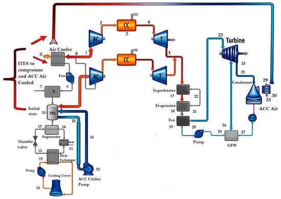
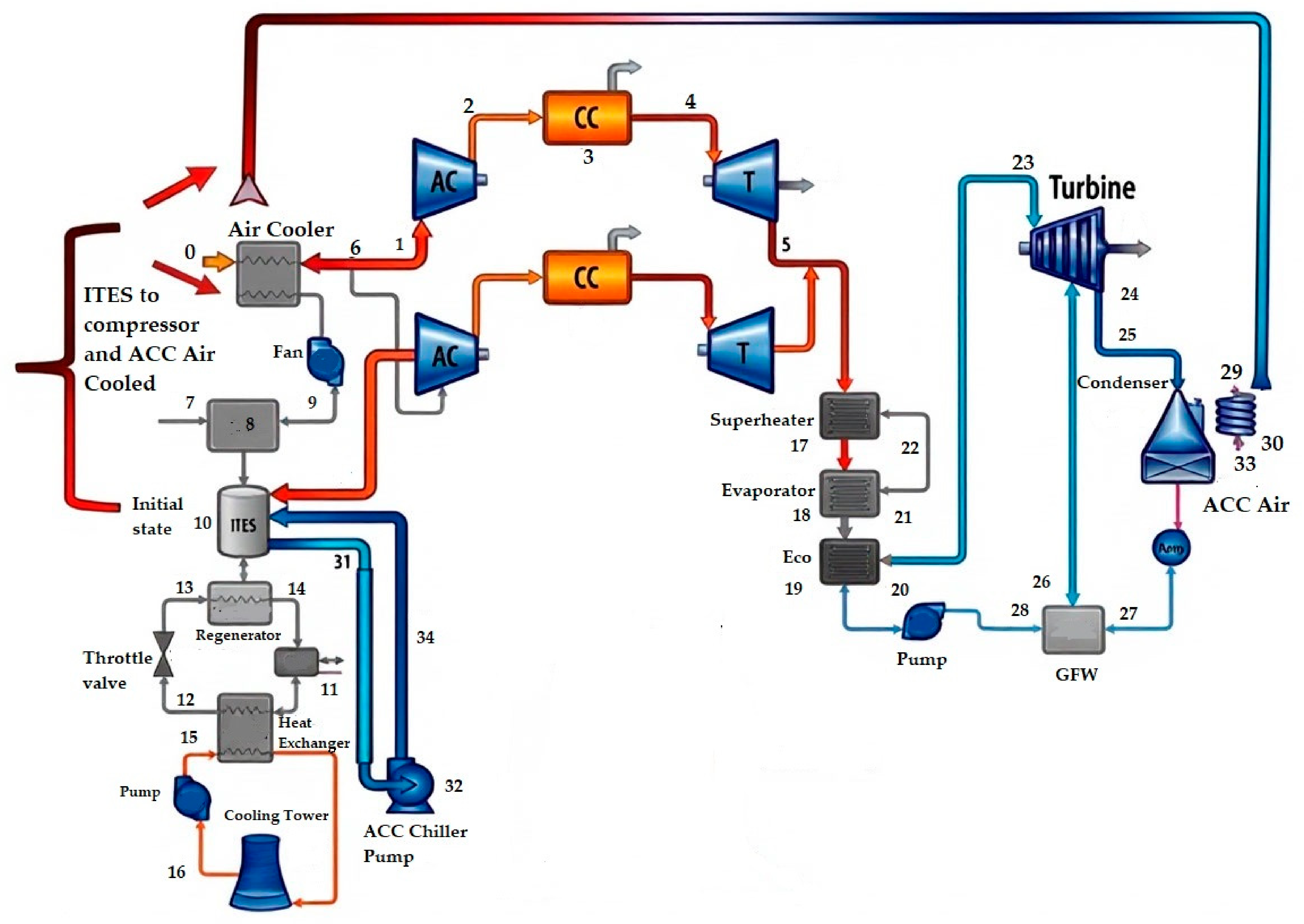
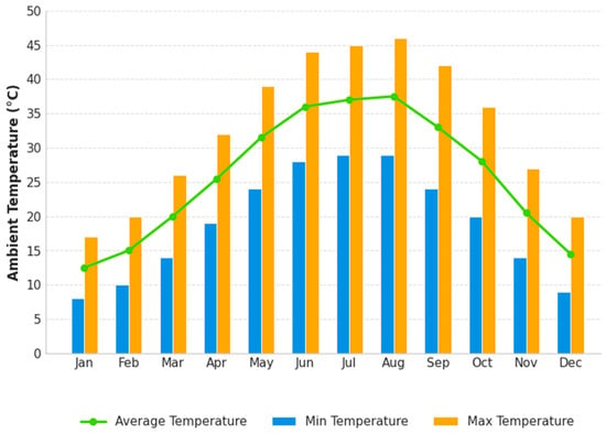
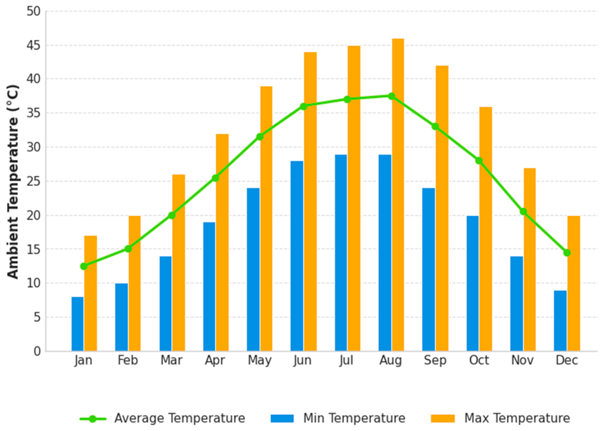
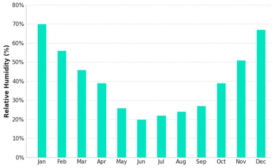
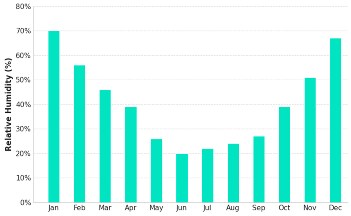
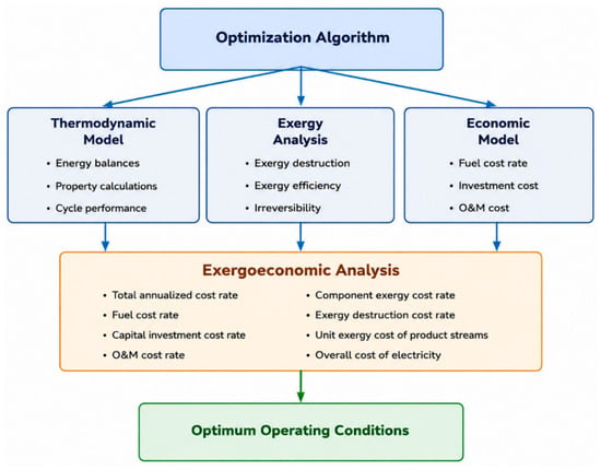
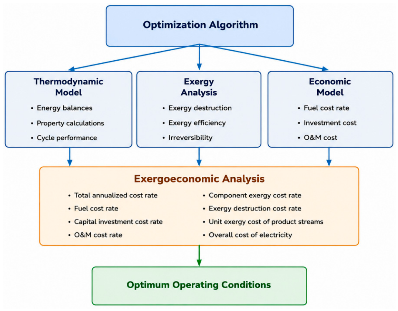
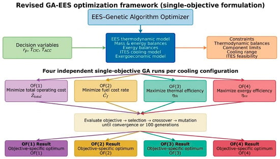
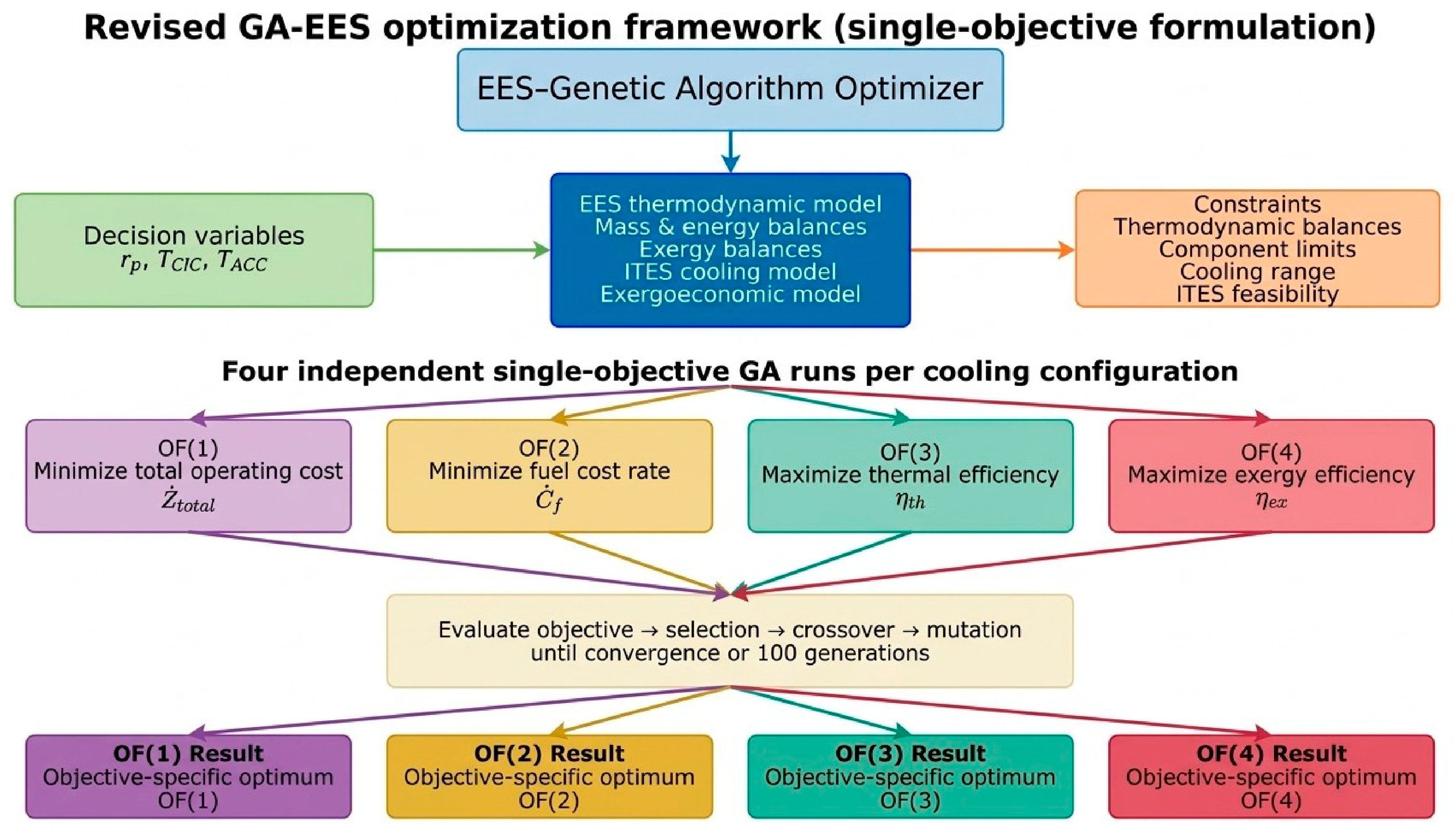
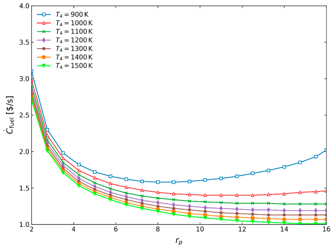
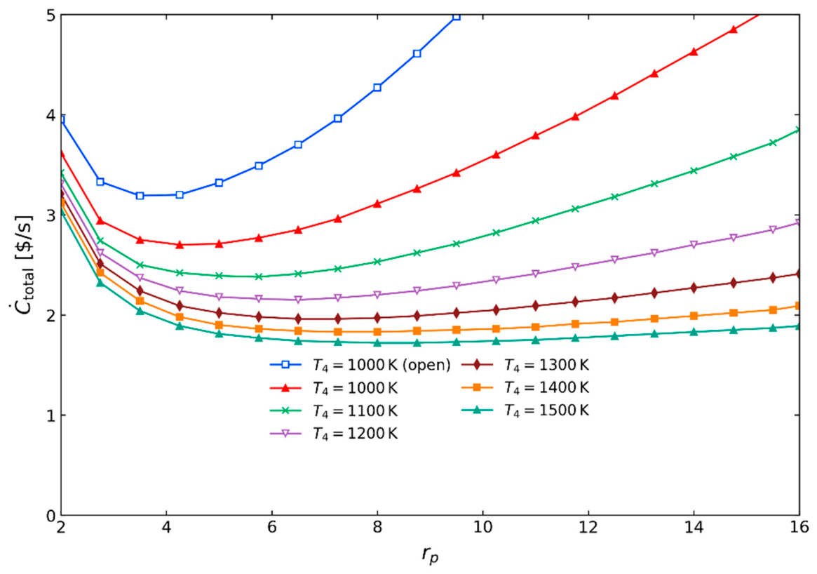
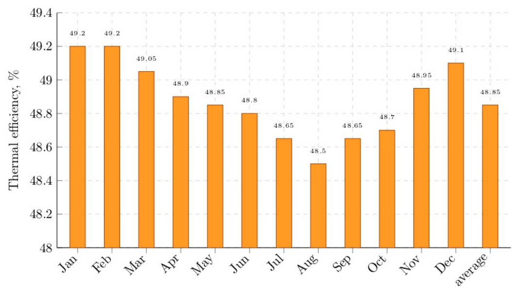
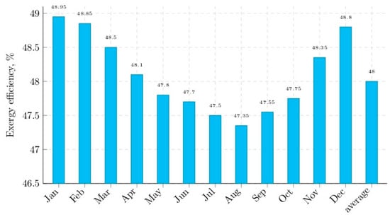
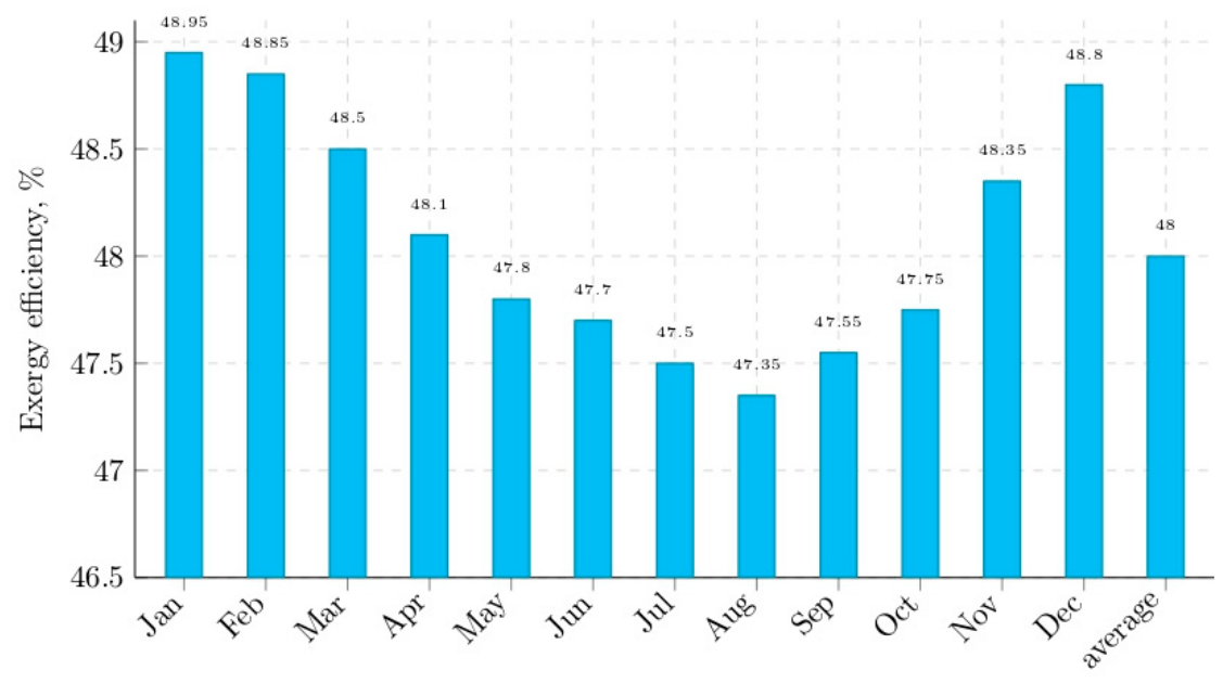
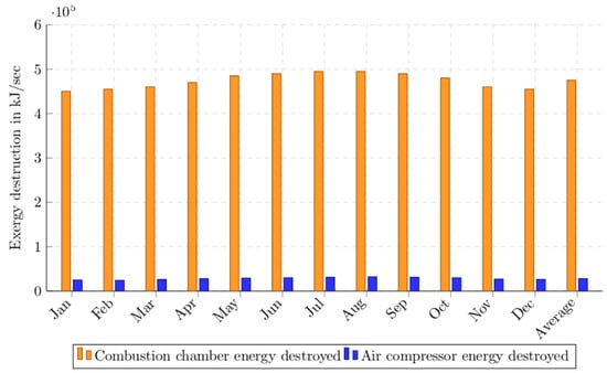
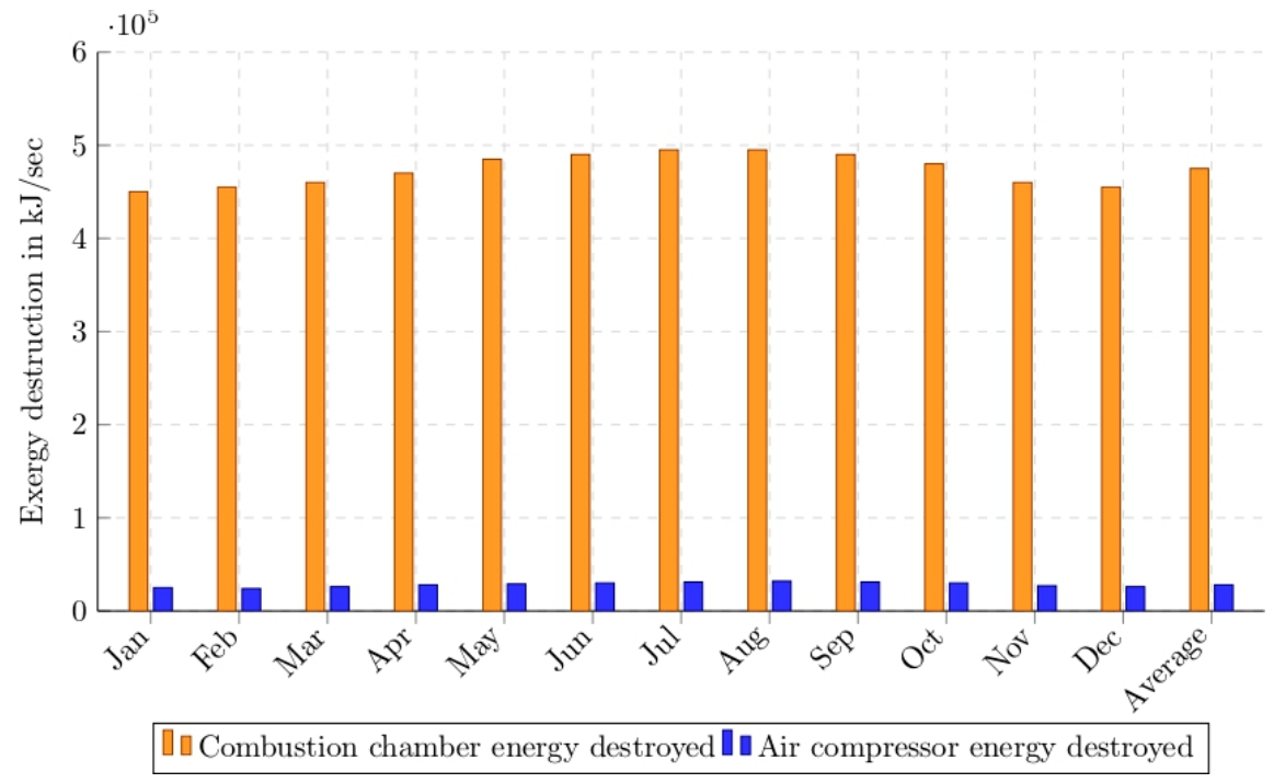
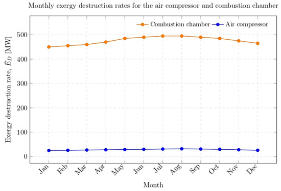
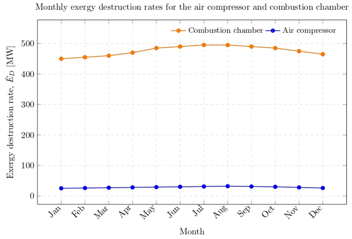
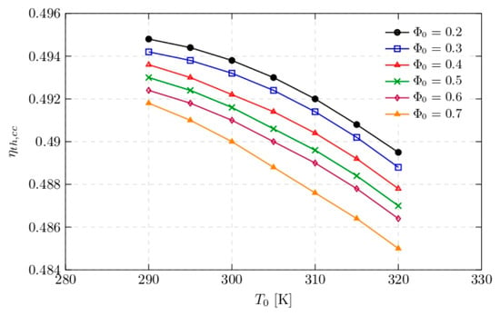
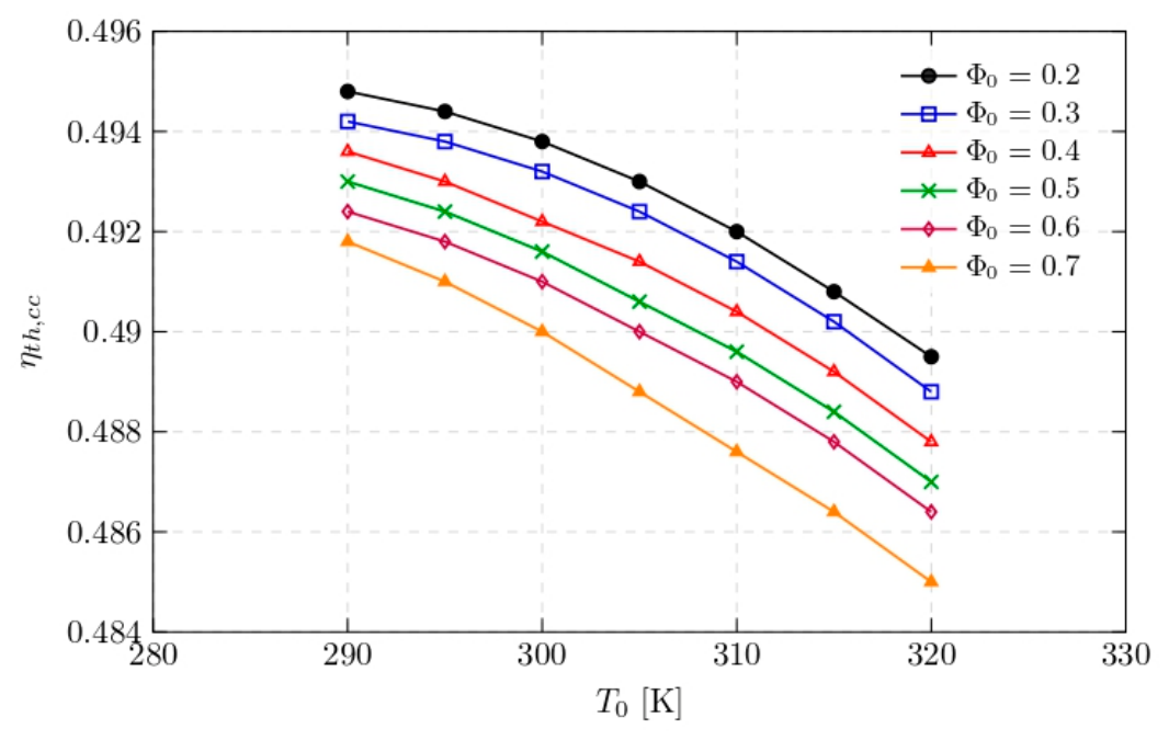
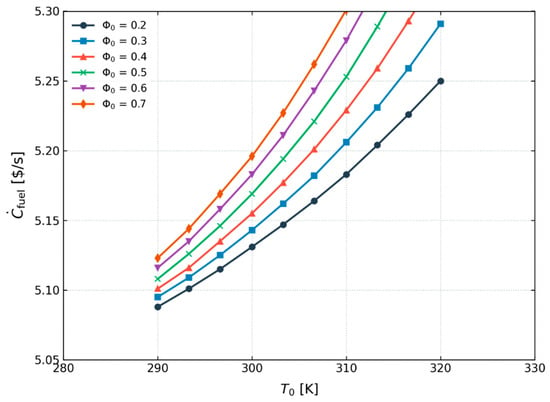
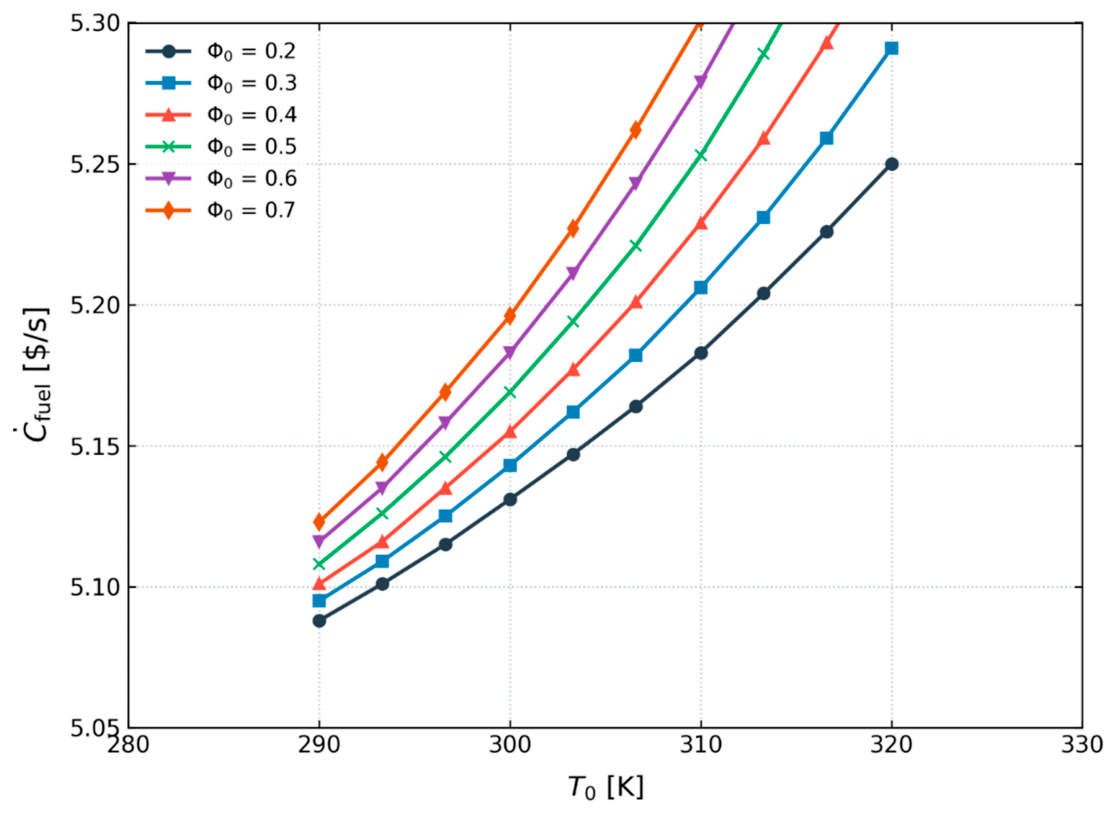
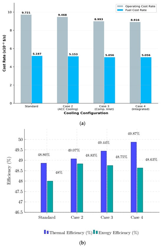
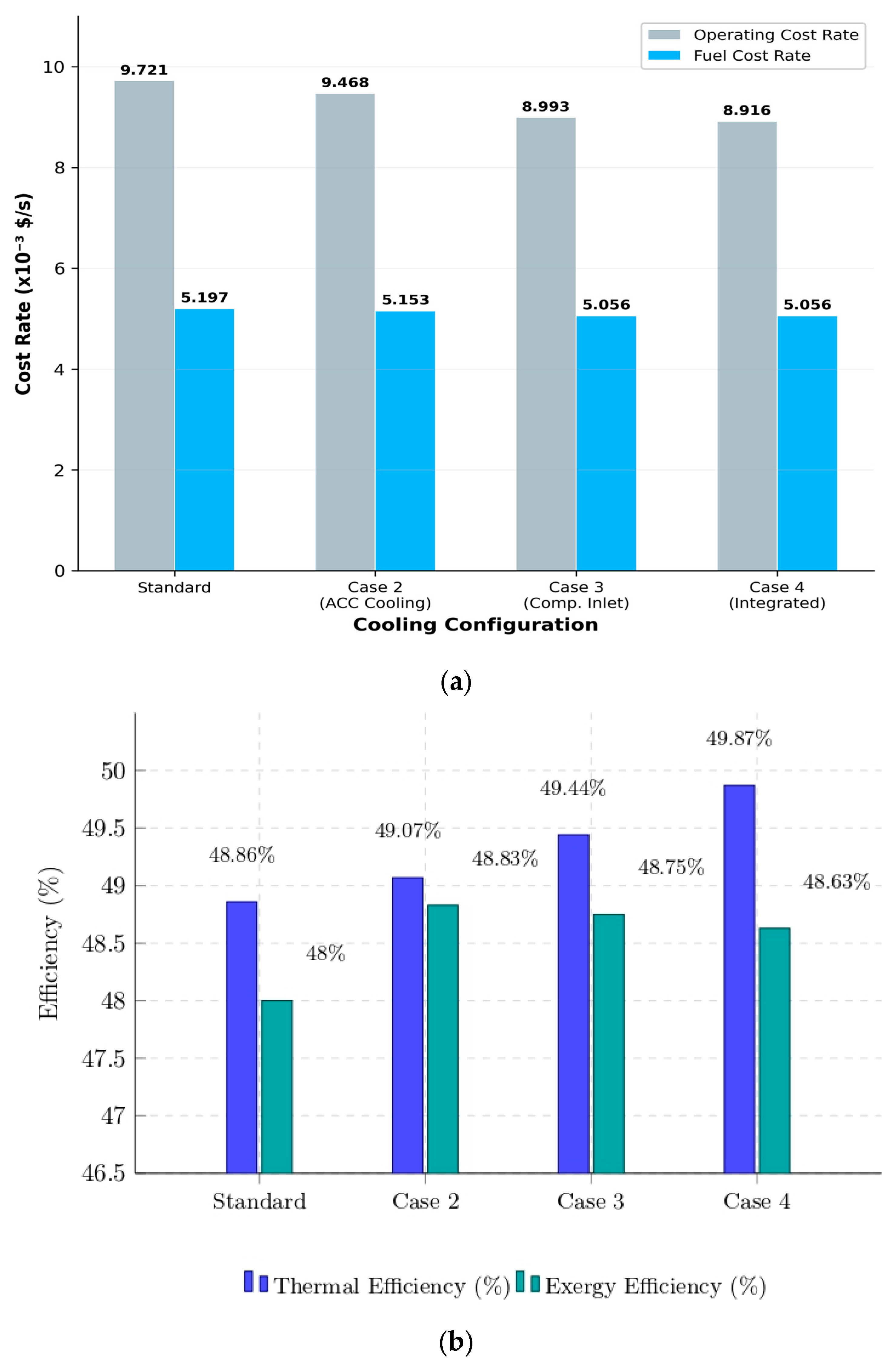
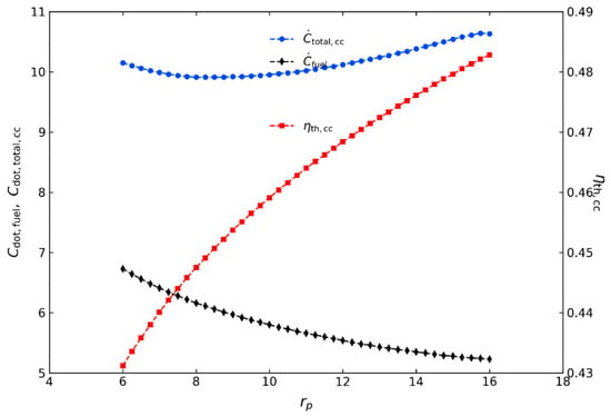
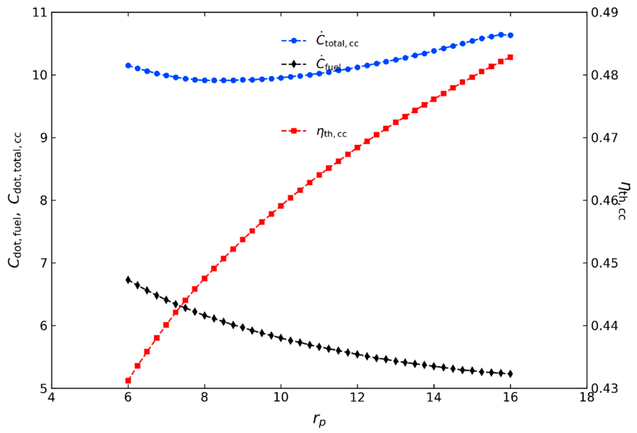
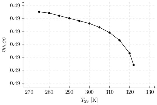
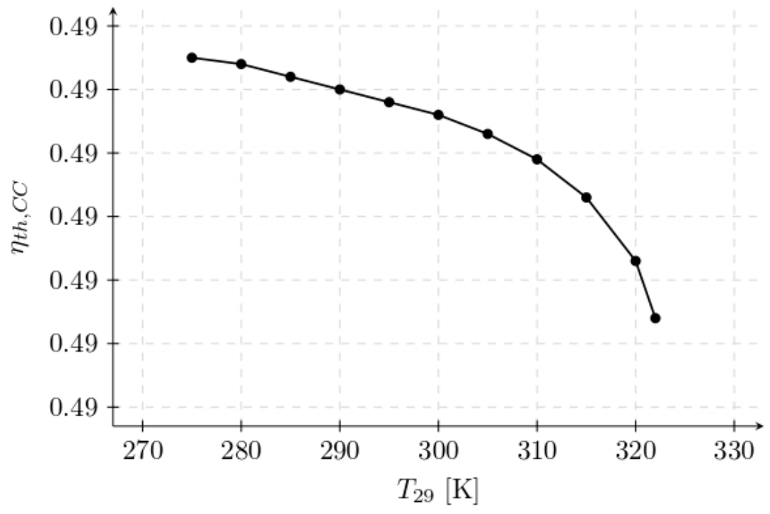

Disclaimer/Publisher’s Note: The statements, opinions and data contained in all publications are solely those of the individual author(s) and contributor(s) and not of MDPI and/or the editor(s). MDPI and/or the editor(s) disclaim responsibility for any injury to people or property resulting from any ideas, methods, instructions or products referred to in the content. |
© 2026 by the authors. Licensee MDPI, Basel, Switzerland. This article is an open access article distributed under the terms and conditions of the Creative Commons Attribution (CC BY) license.