Simulation and Verification of the Driving Resistance of Refrigerated Trucks with Flow Deflectors at Different Vehicle Speeds

Abstract

Air resistance is an important factor affecting the energy consumption of refrigerated-truck transportation. This study combined computational fluid dynamics (CFD) with particle image velocimetry (PIV) to investigate the effects of a cab-mounted flow deflector and vehicle speed on the aerodynamic resistance of a refrigerated truck. A three-dimensional model of the truck was simulated at 50, 70, and 90 km/h with and without the flow deflector. A geometrically scaled PIV model was tested at corresponding model-scale wind speeds and compared with scaled CFD results. The flow deflector reduced the drag coefficient by 14.0–15.0% over the tested speed range, reaching 15.0% at 90 km/h. The downforce increased with vehicle speed, while the reference-area drag coefficient decreased gradually with speed. The mean relative error between the PIV and CFD velocities at ten measurement positions was 4.72% ± 1.63% (mean ± standard deviation), supporting the reliability of the model within the measured front-body region. These results provide a reference for reducing the aerodynamic resistance and energy consumption of refrigerated trucks.

1. Introduction

With the strong demand in the cold-chain market, the number of refrigerated trucks has maintained an annual growth rate of more than 20% for five consecutive years [1]. However, most refrigerated trucks have not yet been equipped with flow deflectors. The aerodynamic characteristics of refrigerated trucks have a significant influence on their road performance. Particularly during high-speed operation, the height difference between the cargo compartment and the cab results in discontinuous vehicle contours and poor airflow streamlining, thereby generating substantial air resistance [2]. Under these circumstances, effective drag-reduction strategies are essential for improving transportation efficiency and reducing fuel consumption.

Recent studies have investigated aerodynamic add-on devices for various commercial vehicles. Connolly et al. [3] comprehensively reviewed passive and active drag-reduction technologies for road vehicles; Levin [4] studied the aerodynamics of a tractor–trailer refrigerated truck and proposed pocket-area add-ons between the tractor and the refrigeration unit, targeting the vertical gap rather than the roof-level flow; Suntaxi [5] numerically assessed a front deflector that modifies the approach flow ahead of a medium-duty freight-truck body; Charles [6] compared drag-reduction devices, including full-height cab-roof fairings, on a simplified truck model; Yuan [7] optimized the roof and body geometry of box-type trucks; Seyhan [8] applied machine learning to truck-trailer drag optimization; and Bardera [9] combined wind-tunnel measurements with PIV to analyze truck drag reduction. One-way FSI analyses of a go-kart spoiler and a utility vehicle splitter have also demonstrated the effectiveness of add-on devices in modifying local flow structures [10], and cab extenders [11] have experimentally reduced the drag of a light commercial vehicle by shortening the cab-to-cargo gap.

These previous designs mainly target a front approach flow, a single cab-to-body step, a full-height roof transition, or a gap between vehicle sections. The refrigerated truck investigated here has a different upper-surface flow path, in which the airflow encounters the cab-to-cargo discontinuity and then the roof-mounted refrigeration unit on the 3200 mm-high cargo compartment. The present cab-mounted curved thin-walled deflector is therefore positioned upstream of both discontinuities and is intended to guide the flow over the front edge of the cargo compartment without closing the cab-to-cargo gap or altering the front face of the vehicle. Consequently, the separation and pressure-recovery behavior around this multiple-discontinuity configuration cannot be directly inferred from conventional single-gap or simplified box-truck cases. In particular, quantitative validation combining high-fidelity CFD with PIV measurements specifically for such refrigerated-truck deflectors remains scarce, leaving a critical gap in understanding the actual flow-field mechanisms under realistic operating conditions.

To address this gap, this study develops a configuration-specific CFD–PIV analysis framework. Scaled PIV measurements of the front-body velocity field are used to assess the CFD predictions before the validated model is applied at 50, 70, and 90 km/h. Baseline and deflector cases are then compared under identical vehicle geometry, computational domain, mesh, boundary conditions, and reference area, enabling the aerodynamic effect of the deflector to be isolated at each speed. Particular attention is paid to the development of the upper-surface flow and the separation region associated with the refrigerated-truck contour. This framework provides a basis for aerodynamic optimization of roof-mounted flow-control devices and extends the evaluation of add-on devices beyond simplified tractor–trailer and box-truck models.

2. Model Construction and Solution

2.1. Solid Model Construction

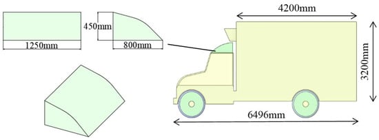
The object investigated in this study was a typical refrigerated truck. The external appearance and basic dimensions of the refrigerated truck are shown in Figure 1. The length, width, and height of the refrigerated truck were 6496 mm, 2500 mm, and 3200 mm, respectively, while the length, width, and height of the flow deflector were 800 mm, 1250 mm, and 450 mm, respectively.

Figure 1. Schematic diagram of the refrigerated-truck structure.

Based on previous studies on the effects of different vehicle components on the drag coefficient and various design strategies on drag reduction [12,13,14,15], as well as the development process of flow deflectors for heavy-duty trucks reported by Zhang Jinzhou [16] and the experimental results obtained by Zhao Lanshui [17], it was found that thin-walled flow deflectors exhibited better performance than solid flow deflectors. In addition, a curved thin-walled structure is generally installed above the cab to regulate the airflow and reduce flow separation in the downstream region. The front curvature is designed to achieve a more reasonable streamlined configuration, while the stabilized airflow above the cargo compartment can reduce the turbulent region at the rear of the vehicle, decrease the wake size, and improve the vehicle dynamic performance.

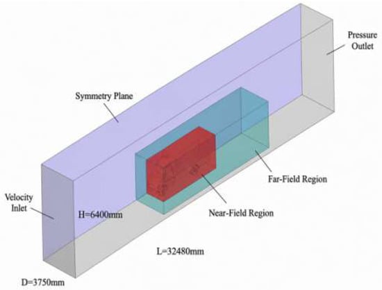
Several complex structures, including the front bumper, engine air intake, and cargo-compartment skirt, exist on the external surface of refrigerated trucks. These complex structures significantly increase the difficulty of numerical simulation and may affect the convergence of the calculation results. Therefore, these details were simplified in the model. Meanwhile, a closed cabin treatment was adopted, and the internal circulation resistance in the total air resistance was neglected [18]. A sketch of the longitudinal section was edited, based on which a near-field region closely surrounding the vehicle body was established. Subsequently, a far-field region was constructed based on the near-field region to simplify the mesh generation process and refine the computational domain around the vehicle, thereby obtaining a more appropriate structure. Since the vehicle model investigated in this study was symmetrical, only half of the computational domain was adopted to reduce the computational workload and improve the solution speed. Finally, the vehicle model was removed to ensure that it was not included in the computational domain. The computational domain consisted of the near-field region, far-field region, and external flow field shell surrounding the vehicle body.

To ensure that the airflow was fully developed during the simulation process, the overall width D, height H, and length L of the computational domain were set to 1.5 times the vehicle width, 2 times the vehicle height, and 5 times the vehicle length, respectively, as no obvious pressure gradient existed in the normal direction of the boundary. The final dimensions of the computational domain were determined to be 32,480 × 3600 × 6400 mm, as shown in Figure 2.

Figure 2. Schematic diagram of the vehicle computing domain.

2.2. Mesh Generation

The built-in meshing module in ANSYS 2021R2 was used to generate the mesh for the refrigerated-truck model. The external shell of the established computational domain was divided into different groups according to the respective regions, so that local mesh refinement could be performed independently for different groups. Meanwhile, the established near-field and far-field shells were used to ensure that the flow near the vehicle could be captured. Local mesh refinement was performed on the model to satisfy the requirements for fitting the model surfaces, and more detailed names could be assigned to different structural components so that the mesh size could be specified independently for each component to optimize the mesh [19]. The specific parameters for local mesh refinement are listed in Table 1.

Table 1. Recommended local grid size.

Region	Minimum Size/mm	Maximum Size/mm	Control Method
Near-field	16	16	Body Of Influence
Far-field	64	64	Body Of Influence
Front of vehicle	4	64	Curvature
Cargo compartment	8	64	Curvature
Chassis	8	64	Curvature
Wheels	8	128	Curvature

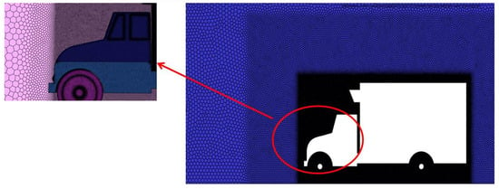
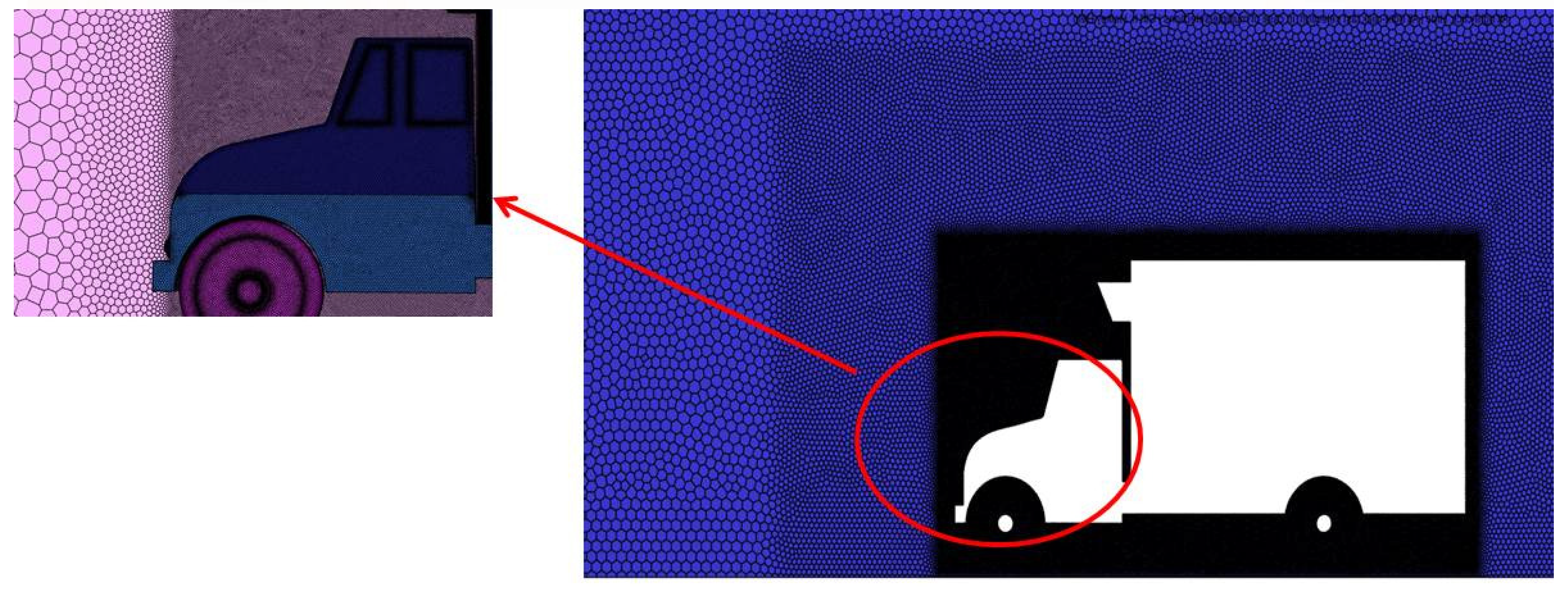
The outer surface of the computational domain was set as a free-slip surface, and the wind pressure and velocity contours on the established symmetry plane were analyzed after the solution was obtained. Since the thickness of the region affected by the airflow in contact with the vehicle surface was very small compared with the characteristic dimensions of the vehicle, a boundary-layer mesh was added before the volume mesh was generated. The boundary-layer mesh was used to simulate and capture the variation in the airflow along the vehicle surface. Five boundary-layer mesh layers were adopted, with a transition ratio of 0.2 and a height of 1.2 mm for each layer, and the mesh was generated only in the vehicle surface region, as shown in Figure 3. After the volume mesh generation was completed, the generated mesh was subjected to a mesh quality check to ensure that the mesh was reasonable and could satisfy the requirements for subsequent computational convergence. For orthogonal quality, the numerical range was 0–1, with 1 representing the best quality and 0 representing the worst quality; a value greater than 0.2 was required. For skewness, a value less than 0.9 which meets the requirements for convergence of subsequent calculations [20].

Figure 3. Schematic diagram of grid size.

Figure 3 shows the surface mesh, local refinement, and five inflation layers. The orthogonal quality remained above 0.2 and skewness remained below 0.9, which satisfies common CFD acceptance criteria [21]. The first-layer height of 1.2 mm was selected so that the SST automatic near-wall treatment maintained the wall-adjacent cells in the wall-function range; the estimated y+ values were approximately 30–100 on the main cab and cargo surfaces. A formal three-grid GCI study and a stored y+ contour were not available in the original dataset; this limitation is stated explicitly in Section 4.3.

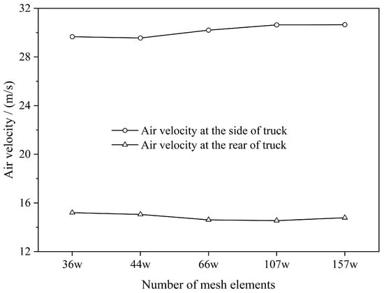
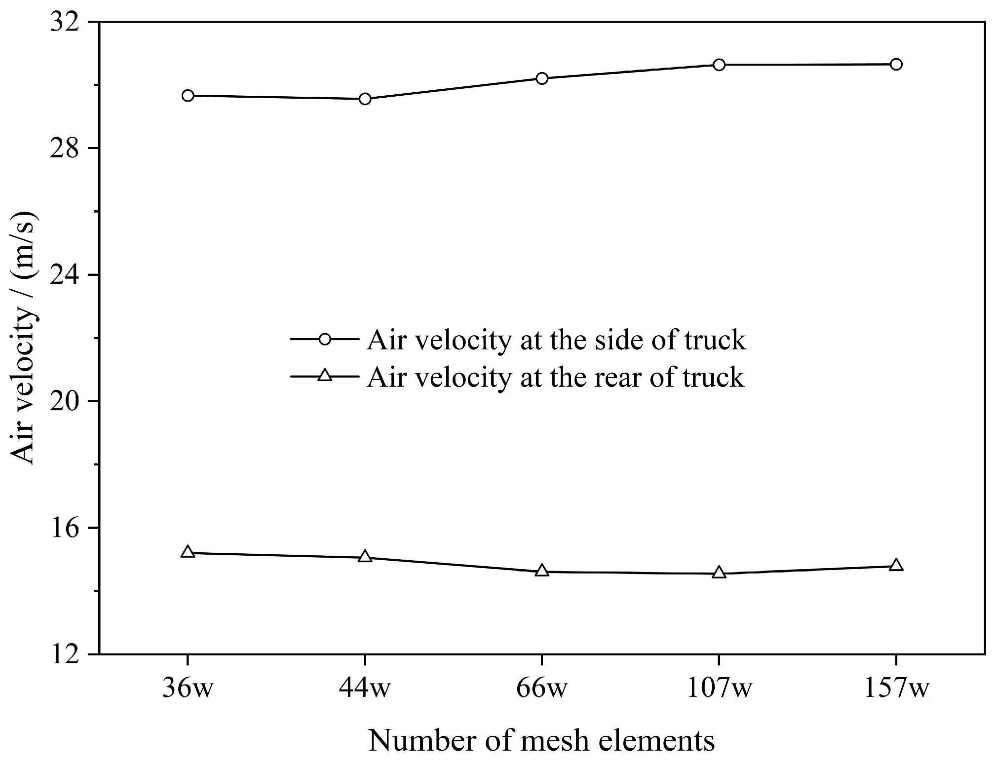
In order to evaluate the mesh size and which parameters are suitable, a grid-independent solution was carried out. The grid numbers tested were 358,284, 443,309, 657,204, 1,066,587 and 1,566,338, respectively, with the corresponding simulation results presented in Figure 4. The average air velocity at the side and rear of truck was analyzed. It can be seen that as the number of grids increases to 1.07 million, the average air velocity at the measurement points tends to be stable, which is consistent with the grid-independent diameter increasing the number of grids but maintaining a similar result. Thus, the 106,6587 grid number is recommended in this study.

Figure 4. Air velocity at the monitoring points varies with the number of grids.

2.3. Governing Equations and Calculation

To facilitate the numerical simulation, the following assumptions were made for the above model:

• The cargo compartment was assumed to have good sealing performance, with no air leakage.
• The air was assumed to be an incompressible gas, satisfying the Boussinesq assumption.
• The air was assumed to be a Newtonian fluid.
• The effects of components such as the vehicle rearview mirrors, air-conditioning radiator, and underhood flow were neglected, and wheel rotation was not modeled. These simplifications are consistent with previous simplified truck aerodynamic studies [4,5] and were adopted to isolate the relative effect of the front-mounted flow deflector while reducing the computational cost.
• The road was flat enough that effects of the vibration on the refrigerated truck can be neglected. Thus, a steady-state environment was assumed.
• The flow was treated as steady and isothermal. Heat transfer, buoyancy, and temperature-dependent property variations were neglected, and the reference air density was kept constant at 1.177 kg/m± for the simulations.

These assumptions were retained because the PIV measurements of the front-body flow were used to verify that the resulting velocity field remained representative for the relative comparison of the two configurations.

Air can generally be regarded as an incompressible fluid when the Mach number is less than 0.3. At vehicle speeds of 50 km/h, 70 km/h, and 90 km/h, the Mach number of the refrigerated truck was less than 0.1; therefore, the external flow field of the refrigerated truck could be regarded as incompressible airflow around the vehicle. Accordingly, treating air as an incompressible fluid can simplify the calculation process [22].

In this study, the model follows the law of conservation of mass. The continuity equation is shown as Equation (1).

$${\displaystyle \frac{\partial \rho }{\partial t}}+\nabla .(\rho V)=0$$

(1)

where ρ is the air density, t is time, and V is air velocity.

During the operation of the refrigerated truck, the external flow field is turbulent and the fluid is incompressible. Therefore, the momentum conservation equation can be expressed using the Navier–Stokes (N-S) equations, as shown in Equation (2).

$$\rho {\displaystyle \frac{\mathit{dv}}{\mathit{dt}}}=\rho F_b-\mathrm{grad}p+\mathrm{div}(2\mathit{\mu S})$$

(2)

where v is the velocity vector, F_b is the mass force per unit mass, grad p is the pressure gradient, div is the divergence, μ is the viscosity coefficient and S is the strain-rate tensor.

In the Reynolds-averaged Navier–Stokes (RANS) formulation used here, v and p represent time-averaged quantities. The momentum balance therefore also contains the Reynolds-stress term which is closed by the SST k-ω model. Because the flow is treated as incompressible, div v = 0 and the compressibility contribution −(2/3)grad(μ div v) in Equation (2) vanishes.

The SST k-ω model blends the k-ω formulation near the wall with the k-ε formulation in the outer region; its transport equations and model constants follow those in study [23] and the SST k-ω model form with consideration of the Reynolds-stress term is shown as follows:

$$\begin{array}{c}{\displaystyle \frac{\partial }{\partial t}}\left(\mathit{\rho k}\right)+{\displaystyle \frac{\partial }{\partial x_i}}\left(\mathit{\rho k}{u}_i\right)={\displaystyle \frac{\partial }{\partial x_j}}\left({\Gamma }_k{\displaystyle \frac{\partial k}{\partial x_j}}\right)+{\overline{G}}_k-Y_k+S_k\end{array}$$

(3)

$${\displaystyle \frac{\partial }{\partial t}}\left(\mathit{\rho \omega }\right)+{\displaystyle \frac{\partial }{\partial x_i}}\left(\mathit{\rho \omega }{u}_i\right)={\displaystyle \frac{\partial }{\partial x_j}}\left({\Gamma }_{\omega }{\displaystyle \frac{\partial \omega }{\partial x_j}}\right)+G_{\omega }-Y_{\omega }+D_{\omega }+{\mathrm{S}}_{\mathsf{\omega }}$$

(4)

In these equations, $\overline{G_k}$ represents the generation of turbulence kinetic energy due to mean velocity gradients. G_ω represents the generation of ω. Γ_k and Γ_ω represent the effective diffusivity of k and ω, respectively. Y_k and Y_ω represent the dissipation of k and ω due to turbulence. D_ω represents the cross-diffusion term. S_k and S_ω are user-defined source terms.

2.4. Aerodynamic Characteristics of the Vehicle

The resistance encountered by a vehicle during operation includes rolling resistance, air resistance, grade resistance, and acceleration resistance. At 50–90 km/h, rolling resistance is not negligible in the absolute road load, but it depends mainly on vehicle mass, tire–road interaction, and tire pressure and is essentially unchanged when a flow deflector is added. Because this study evaluates the aerodynamic effect of the deflector, aerodynamic drag is isolated as the comparison metric; total road load would require adding rolling resistance [24]. Air resistance becomes dominant at approximately 100 km/h, while the selected 50–90 km/h range covers typical refrigerated-truck operating speeds and allows the transition in deflector effectiveness to be examined.

Air resistance has a significant influence on vehicle performance. A lower drag coefficient indicates that the vehicle is less affected by air resistance at high speeds, whereas a higher drag coefficient results in greater resistance at high speeds. Therefore, a lower drag coefficient is more favorable for vehicle operation. In general, vehicles with a more streamlined shape have a lower drag coefficient C_d. Under no-wind conditions, the drag coefficient was calculated using the formula shown in Equation (5).

$$F_w={\displaystyle \frac{C_{d}A{u}_{\alpha }^2}{21.15}}$$

(5)

where F_w is the vehicle driving resistance, A is the frontal projected area of the vehicle, and u_α is the vehicle traveling speed.

In Equations (5) and (6), u_α is expressed in km/h and A is the frontal projected reference area. The projected area obtained from the CAD geometry was A = 4.12 m². The coefficient 21.15 is the conventional value obtained from 25.92/1.225, where 1.225 kg/m³ is the standard reference air density at 15 °C. Thus, 21.15 is deliberately used for the analytical drag equations, whereas the CFD solver uses ρ = 1.177 kg/m³ at 27 °C.

Equation (5) can be rearranged to obtain Equation (6).

$$C_d={\displaystyle \frac{21.15F_w}{\mathit{\rho A}{u}_{\alpha }^2}}$$

(6)

2.5. Solver and Boundary Condition Calculation Settings

Under actual operating conditions, a typical refrigerated truck was considered to travel on a highway. The ambient temperature was assumed to be 27 °C, and the simulation reference air density was therefore set to 1.177 kg/m³. The frontal projected reference area used to calculate the drag coefficient was A = 4.12 m². The vehicle was assumed to travel at a constant speed, and the influence of external wind was neglected so that the flow field remained steady and isothermal. The turbulent intensity (I) was calculated using Equation (7), while the Reynolds number (Re) was calculated using Equation (8).

$$I=0.16{\left(\mathrm{Re}\right)}^{-1/8}$$

(7)

$$\mathrm{Re}={\displaystyle \frac{\mathit{\rho vd}}{\mu }}$$

(8)

where μ is the dynamic viscosity, and d is the characteristic length.

For the full-scale model, the Reynolds number based on vehicle height ranged from approximately 2.8 × 10⁶ to 5.1 × 10⁶ at 50–90 km/h, confirming turbulent flow. Considering the relatively high computational accuracy of the k-ω model for complex near-wall flows, the SST k-ω model with curvature correction was adopted for the calculation [19]. Gravity was considered in the solver; a pseudo-transient formulation of the pressure-based coupled solver was used, and the upwind scheme was changed to the second-order upwind scheme to improve accuracy.

The vehicle in the computational domain was kept stationary. According to the actual operating conditions of refrigerated trucks during transportation, vehicle speeds of 50 km/h, 70 km/h, and 90 km/h were selected as the initialization parameters. The turbulence intensity and turbulent viscosity ratio at the inlet were set to 0.5% and 2, respectively. A pressure outlet was specified at the outlet, with the turbulence intensity and turbulent viscosity ratio selected accordingly. Since the turbulence at the outlet was connected to the atmosphere, the settings were kept consistent with those at the inlet. The ground was set as a slip wall, with its velocity set equal to the incoming flow velocity. Since the computational domain was sufficiently large and the kinetic energy of the airflow had already dissipated, the tunnel surface was set as a specified shear surface with a pressure of 0 Pa to simulate a free-slip wall [19]. No settings were required for the symmetry plane. The detailed boundary conditions are listed in Table 2.

Table 2. Setting of boundary conditions.

Region	Parameter Settings
Inlet	Velocity: 50 km/h, 70 km/h, 90 km/h Turbulence intensity: 0.5% Turbulent viscosity ratio: 2
Outlet	Pressure outlet: 0 Pa Turbulence intensity: 0.5% Turbulent viscosity ratio: 2
Ground	Along the positive X-direction Velocity magnitude: same as that at the inlet
Outer wall of the flow field	Specified shear surface stationary

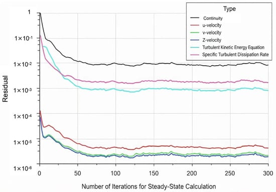
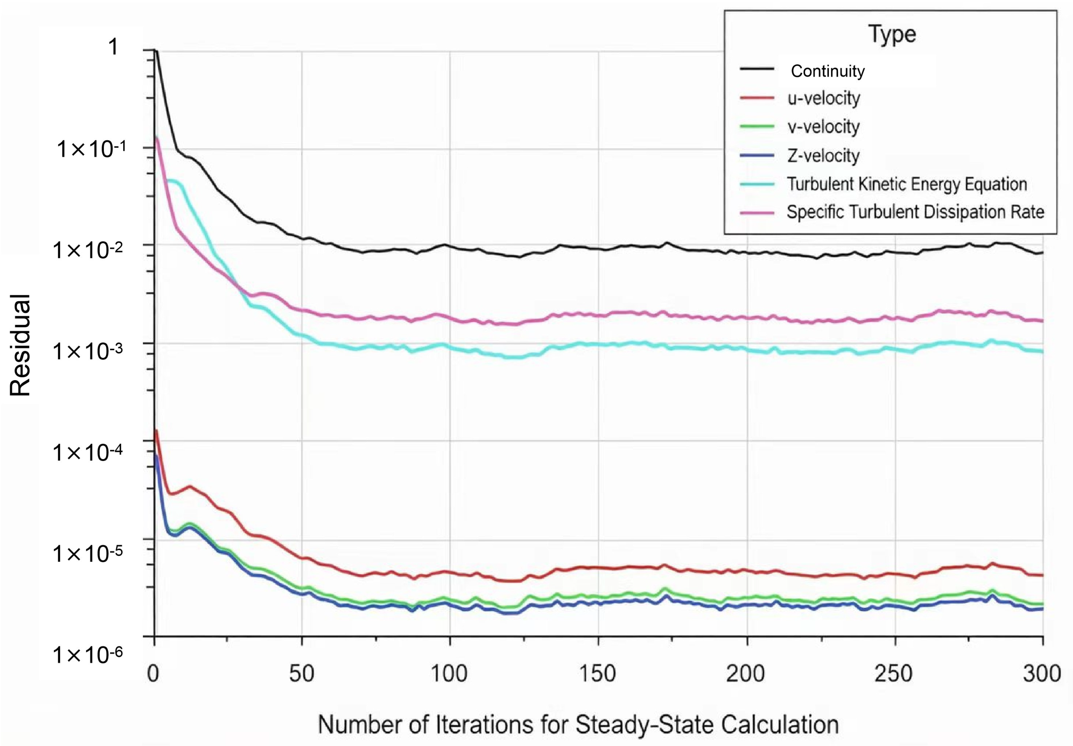
The entire flow field was initialized using the FMG (Full-Approximation Storage (FAS) Multigrid) method. Convergence was assessed using three criteria: (i) the scaled residuals for continuity and momentum decreased and stabilized, (ii) the monitored integral drag force changed by less than 0.1% over the final 100 iterations, and (iii) the global mass imbalance remained below 0.1%. Up to 600 iterations were allowed; these criteria were satisfied at approximately 300 iterations, as shown in Figure 5, and additional iterations produced no material change in the drag results.

Figure 5. The number of iterations and the variation in residual values.

3. Experimental Verification Using PIV

3.1. Measurement Principle of PIV

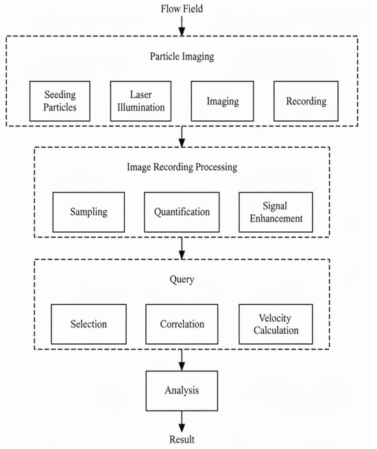
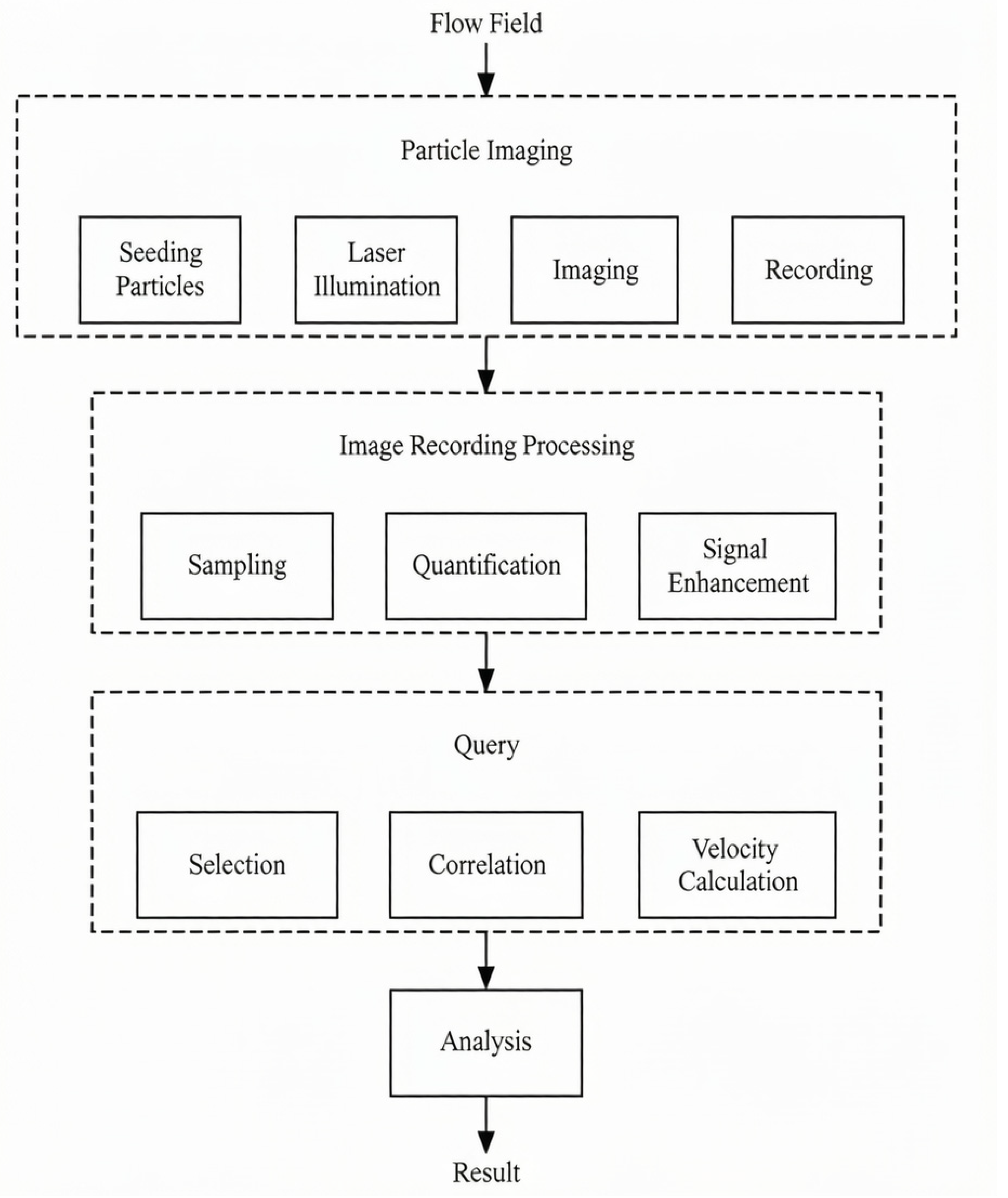
PIV originated from Laser Scattering Velocimetry. Its earliest application in fluid measurement was reported by Barke D, et al. for measuring the velocity of laminar flow in pipelines [25]. In PIV, tracer particles are dispersed into the measurement region and illuminated using a laser, after which a high-speed camera is used to capture two images of the tracer particles at different positions within a given time interval. The instantaneous velocity information of the tracer particles in the measurement field is then obtained through cross-correlation calculations and used to represent the flow velocity of the fluid, thereby obtaining the velocity field of the measured fluid [26]. The basic procedure of the PIV measurement technique is shown in Figure 6.

Figure 6. PIV measurement step diagram.

3.2. Construction and Validation of the PIV Experimental Platform

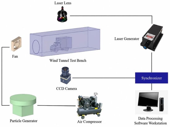
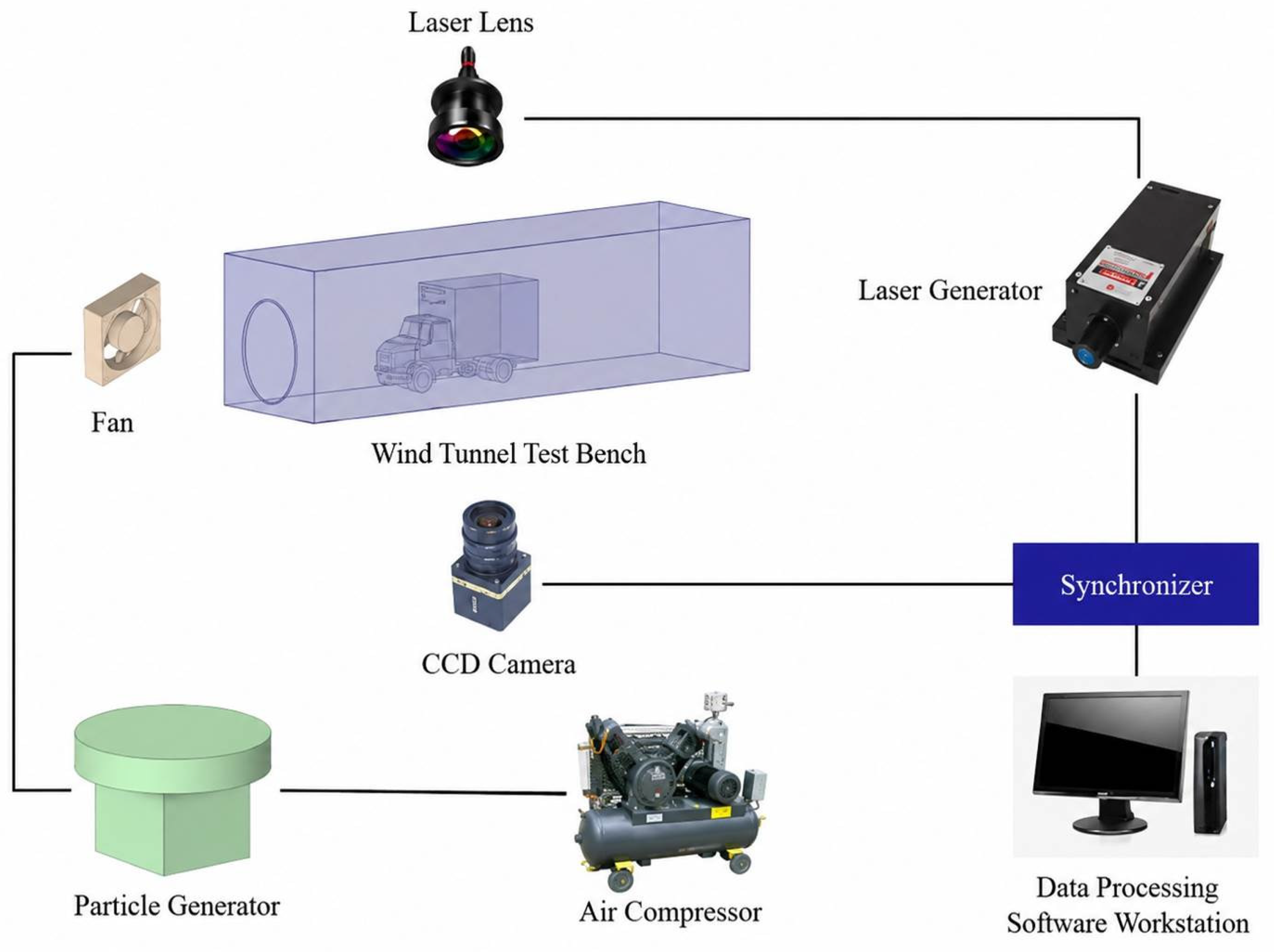
By introducing PIV technology and combining automotive aerodynamics with PIV measurements [27,28,29,30], the actual flow conditions around the vehicle were obtained and compared with the numerical simulation results for validation. The PIV experimental platform is shown in Figure 7.

Figure 7. Schematic diagram of the PIV experimental system.

The Dynamic Studio 6.0 software was used for image calibration, image acquisition, data collection, and post-processing. A calibration plate was used to calibrate the positional information in the images. After the measurement results were obtained, irrelevant, reflective, and blurred regions in the measurement area were removed, leaving only the region surrounding the vehicle model. Subsequently, correlation algorithms and vectorization processing were applied to the images. The main components and parameters of the test system are listed in Table 3.

Table 3. The main components of the measurement system include equipment models and parameters.

Component	Model	Parameter
Wind-tunnel test platform	—	Length × width × height: 500 mm × 130 mm × 120 mm
Air compressor	1500 W–30 L	Power: 1500 W Pressure: 0.8 MPa Air displacement: 150 L/min
Particle generator	FT700CE	Maximum pressure: 0.4 MPa
Tracer particles	Olive oil droplets	Particle size: 3 μm Density: 0.91 g/m3
Laser generator	DualPower TR	Working medium: Nd:YAG nmLaser wavelength: 532 nm Maximum pulse energy: 500 mJ Beam duration: 4 ns Light sheet thickness: 1 mm
CCD camera	FlowSence EO-4M	Resolution: 2048 pixels × 2048 pixels

The PIV experiment used a geometrically scaled model (1:53) of the same truck. The model-scale wind speeds were obtained by converting the full-scale operating speeds using the geometric scale ratio, and a corresponding scaled CFD case was generated with the same inlet velocities and boundary conditions for each setting reported in Table 4. Table 4 therefore compares model-scale PIV data with model-scale CFD data, not directly with the 50–90 km/h full-scale cases.

Table 4. Comparison between PIV experimental data and simulation data. Note: After removal of one duplicated row, ten independent measurement positions were used. Relative error is the arithmetic mean of the ten position-wise errors; ± denotes one sample standard deviation.

PIV Experimental Wind Speed/m/s	Simulation Wind Speed/m/s	Relative Error/%
0.899	0.946	5.16
0.913	0.955	4.57
0.906	0.962	6.19
0.900	0.967	7.45
0.922	0.972	5.49
0.932	0.981	5.28
0.943	0.984	4.41
0.968	0.992	2.48
1.092	1.113	1.94
1.082	1.128	4.22
Mean ± SD	0.956 ± 0.072	1.000 ± 0.065; error 4.72 ± 1.63%

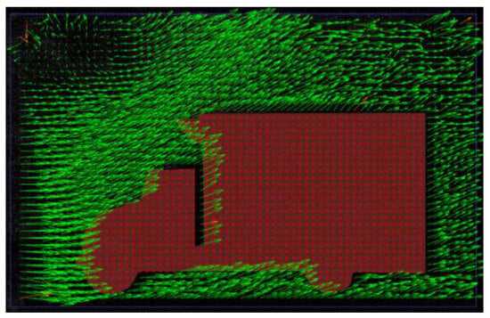
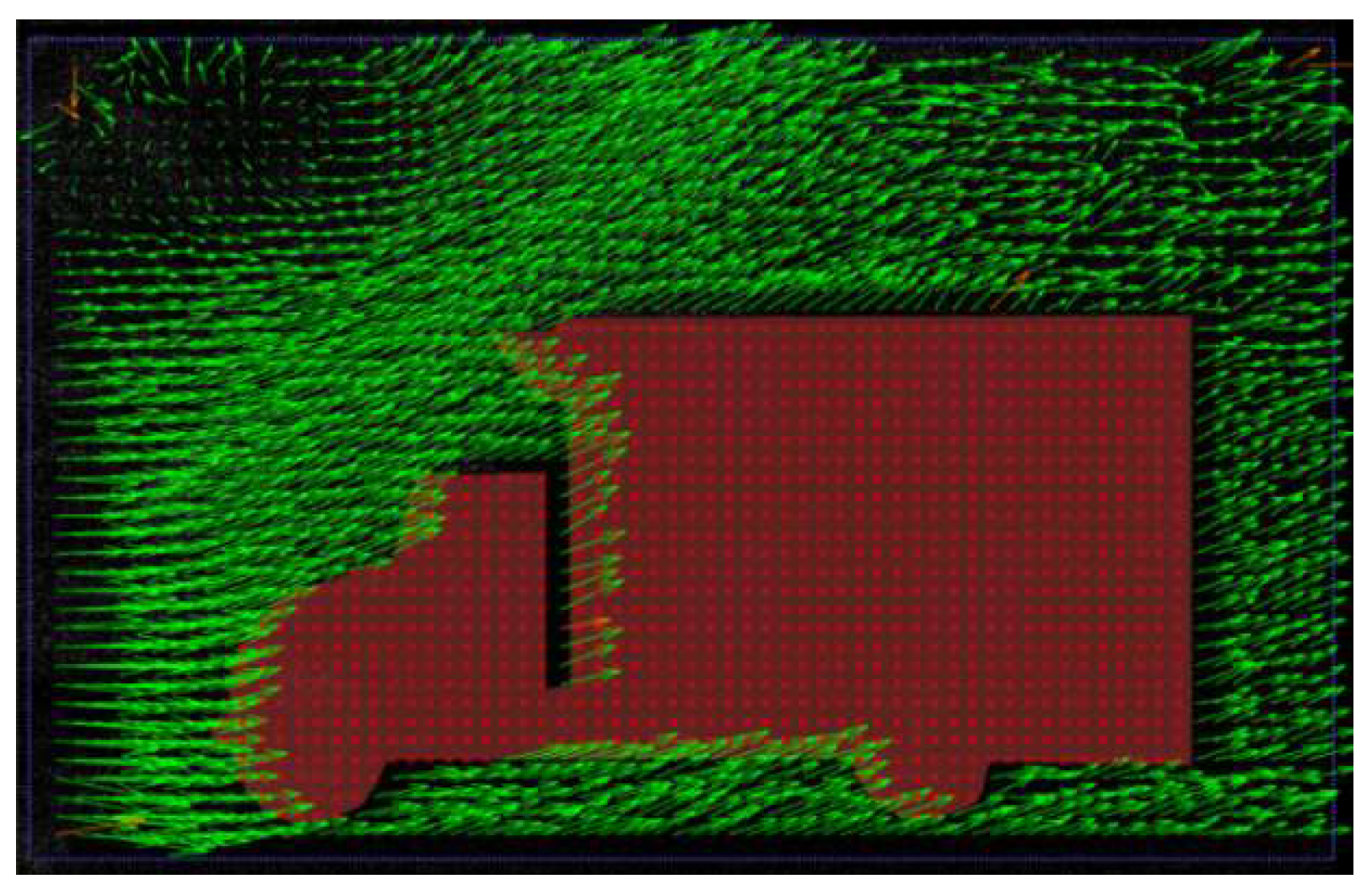
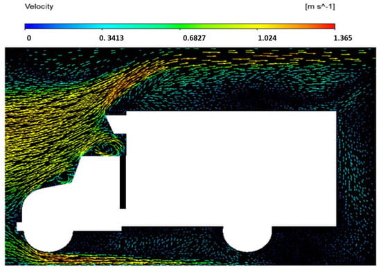
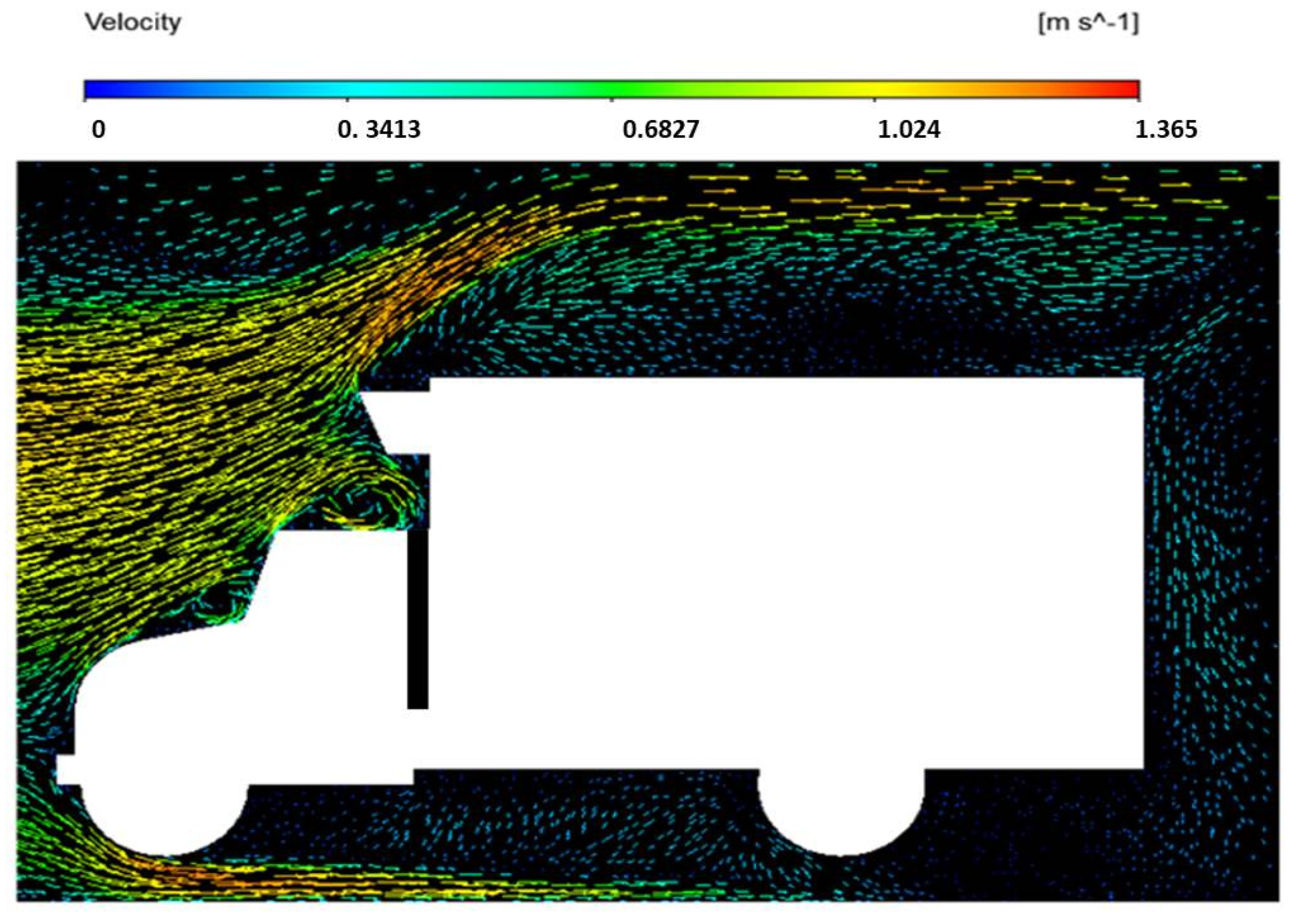
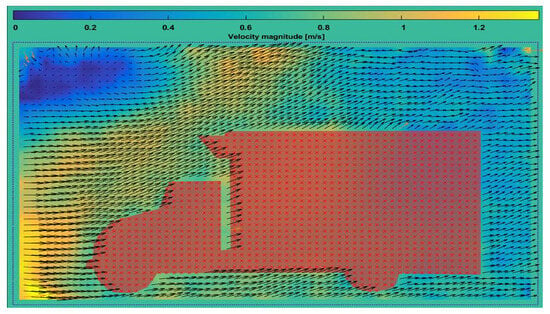
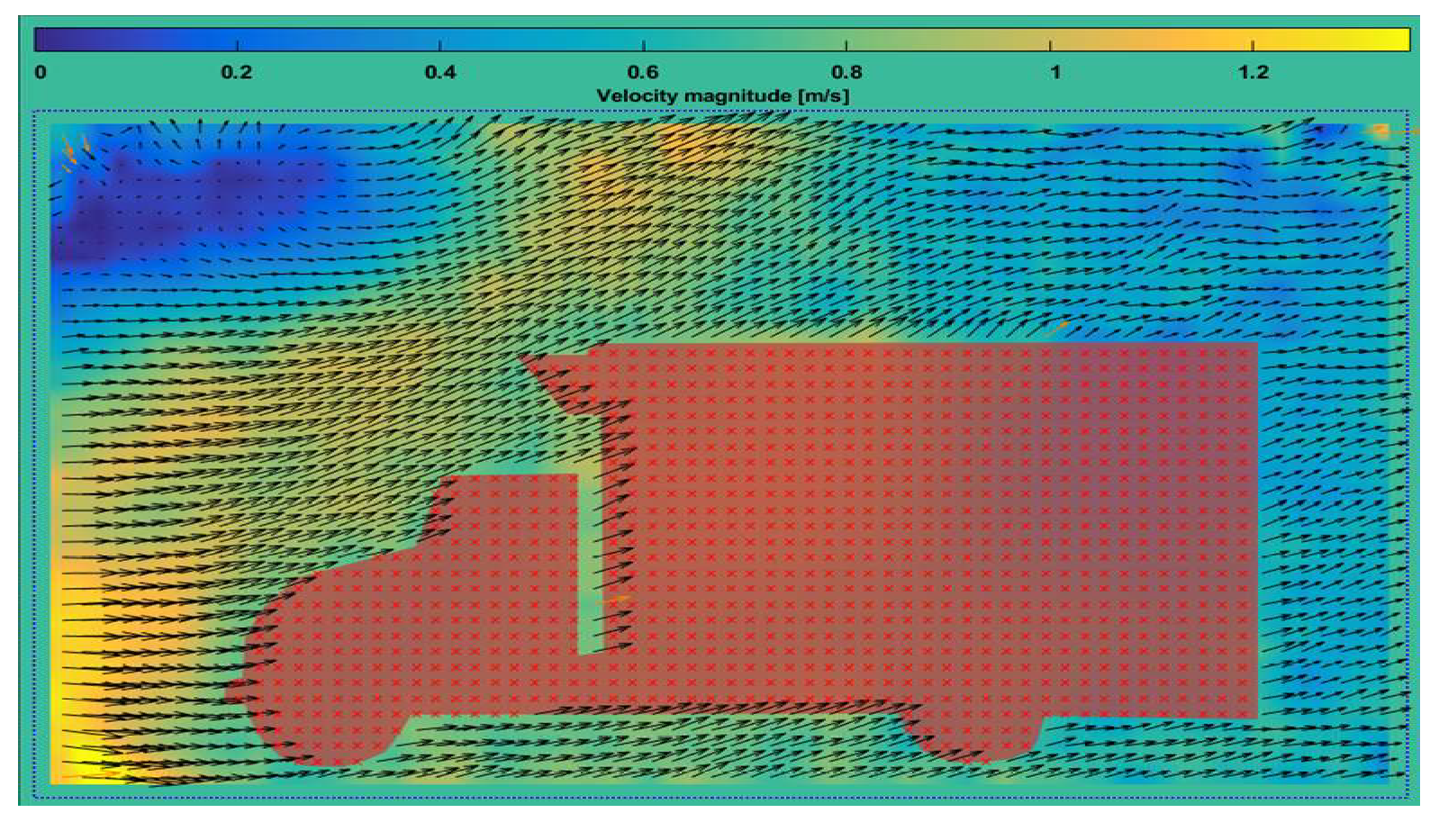
The vector field contours of the airflow around the vehicle during operation were obtained using the PIV equipment, as shown in Figure 8. The Pivlab module in MATLAB 2020b was then used to visualize the streamlines of the velocity field. After processing, the airflow velocity contours were obtained and compared with the velocity contours obtained from the numerical simulation, as shown in Figure 9 and Figure 10.

Figure 8. Vector contours captured by the PIV equipment.

Figure 9. CFD vector flow field contours.

Figure 10. PIV flow field vector contours.

A vertical line segment 20 cm upstream of the model and perpendicular to the flow was selected to compare the wind speed data, as shown in Table 4. The relative error was calculated as ε = (1/n)Σ|u_PIV − u_CFD|/u_PIV × 100%. After removal of one duplicated row, ten valid positions gave a mean relative error of 4.72% with a standard deviation of 1.63%, demonstrating the reliability of the model in the measured front-body region. The velocity along the selected line fluctuated more in the PIV experiment than in the CFD simulation because of unsteady wind conditions and measurement uncertainty, but its decreasing trend was consistent with the simulation. This line does not fully validate the rear wake or the separation region; that limitation is discussed in Section 4.3.

4. Results and Analysis

After the solution was set, force calculations were performed in the negative X-direction of the computational domain. Since the vehicle was subjected only to air resistance in this study, all forces acting in this direction were considered to be the driving resistance of the vehicle. The calculated driving resistance of each component of the model at different traveling speeds is presented in Table 5. It can be seen from the table that the cargo compartment and the cab were subjected to most of the resistance, while the resistance acting on the cab varied significantly with the traveling speed. In the subsequent calculations, the driving resistance acting on the cab and cargo compartment was taken as the air resistance acting on the vehicle in the forward direction.

Table 5. Driving resistance of each component at different speeds.

Component	50 km/h Resistance/N	70 km/h Resistance/N	90 km/h Resistance/N
Tires	8.67	11.42	17.84
Chassis	17.69	24.66	38.46
Cargo compartment	305.29	490.90	829.73
Cab	103.70	243.62	329.83

Table 5 reports the negative-X force contributions obtained by integrating the pressure and viscous forces over the corresponding vehicle components. The tire and chassis entries are provided only to show the component partition; the aerodynamic driving resistance used in Equation (3) is the sum of the cab and cargo-compartment contributions. The same reference area, A = 4.12 m², was used for every speed and for both configurations.

4.1. Analysis of Finite Volume Simulation Results of the Initial Model

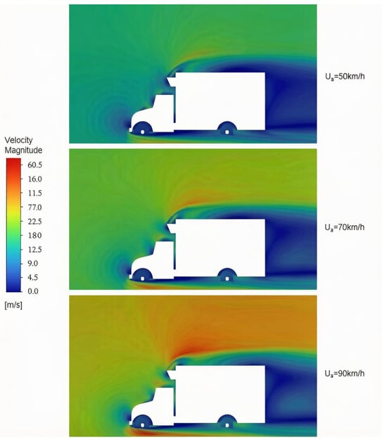
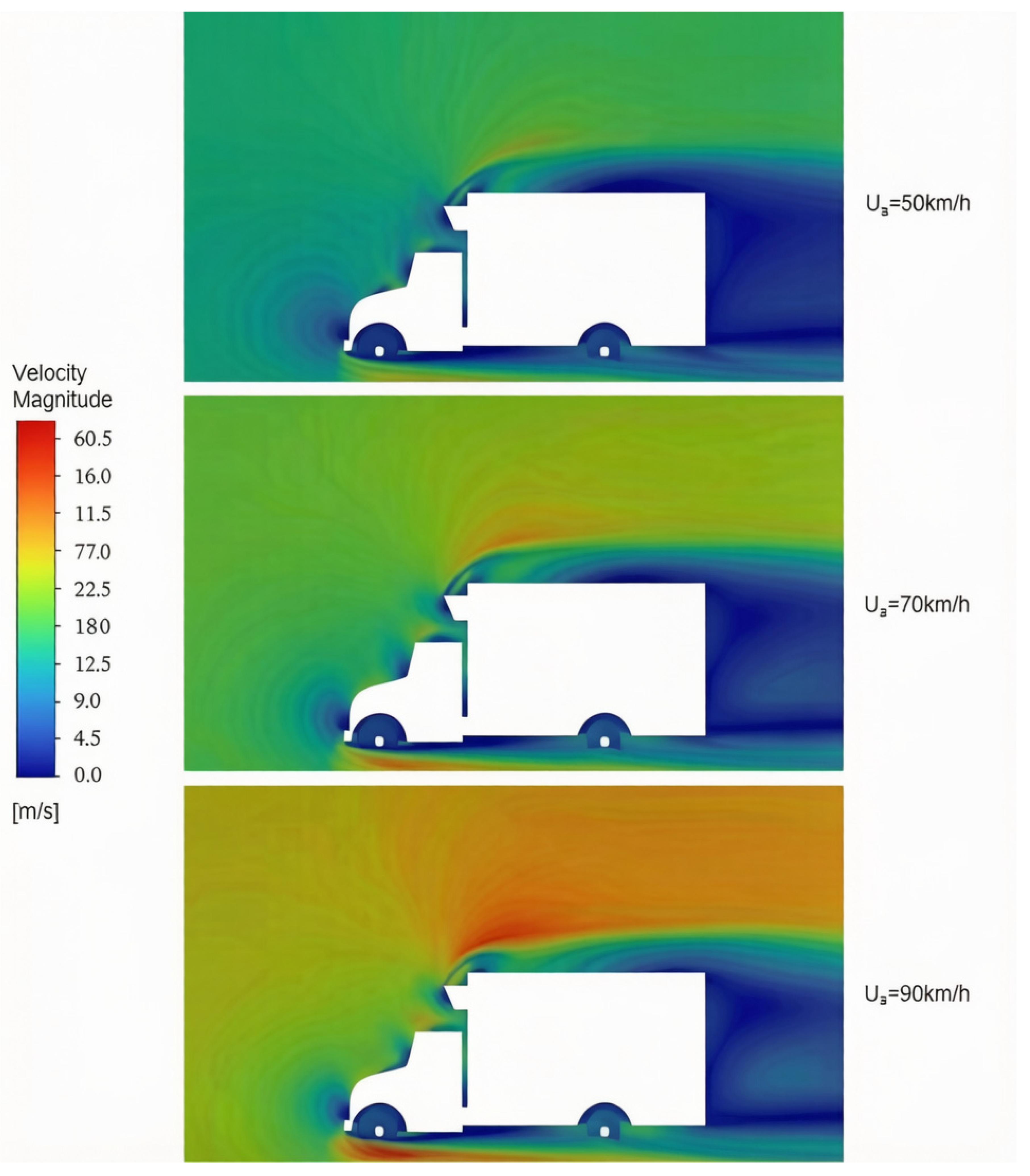
The simulation results of the model without a flow deflector at different traveling speeds were extracted for comparative analysis. As the traveling speed increased, flow separation occurred at the front end of the cargo compartment, resulting in significant changes in the wind speed gradient at the front end of the cargo compartment, while the maximum velocity of the external flow field increased from 23.56 m/s to 47.64 m/s. The airflow directly impinged on the exterior of the cargo compartment at its front end, resulting in flow stagnation, which was manifested as the blue region at the front of the vehicle in Figure 11. Meanwhile, a flow recirculation region appeared behind the cargo compartment and gradually increased in size. The airflow in this region moved in the direction opposite to the overall flow direction, resulting in a significant increase in the driving resistance acting on the cargo compartment.

Figure 11. Velocity contours of the overall vehicle of the original model at different traveling speeds.

4.2. Finite Volume Simulation Results of the Model with a Flow Deflector Installed

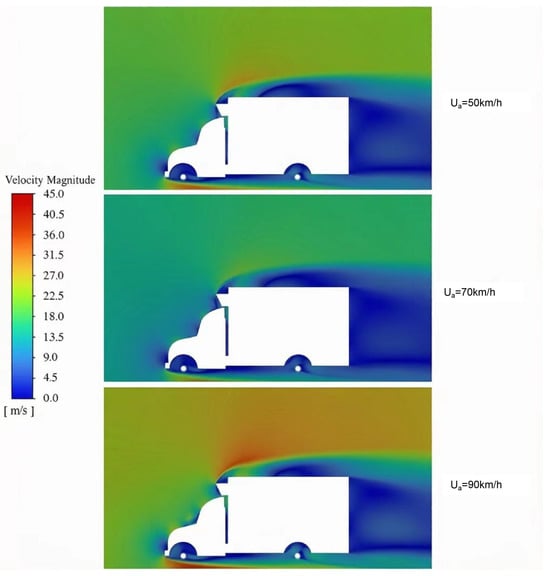
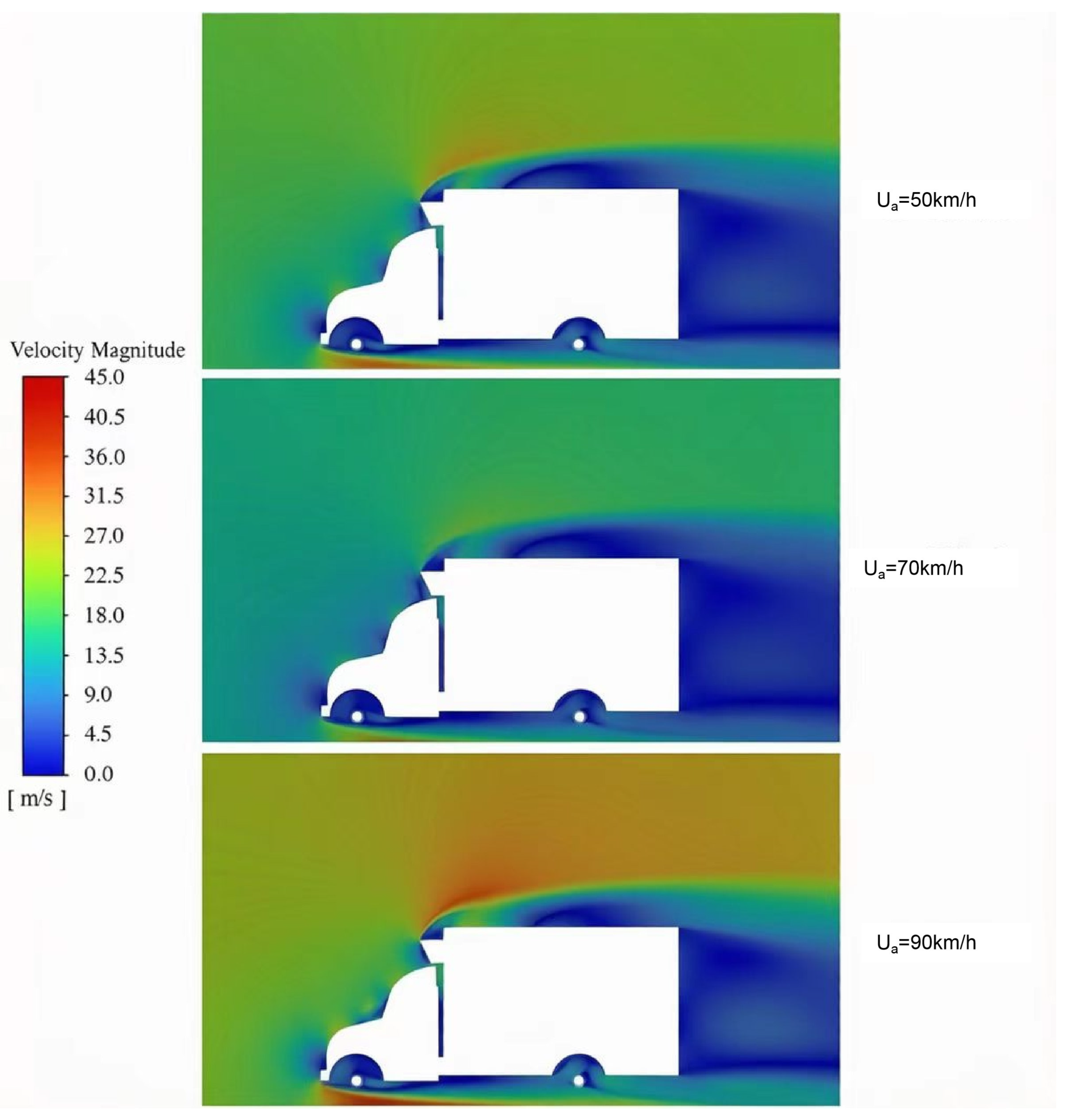
The simulation results of the vehicle model with a flow deflector installed were analyzed, and the results are shown in Figure 12. It can be observed from the velocity contours that a relatively smooth transition region was formed above the cab, which weakened the flow separation occurring between the top of the cab and the edge of the cargo compartment. The separated airflow exhibited a relatively stable distribution, and it partially offset the wake at the rear end of the cargo compartment. The variation in the wind speed gradient at the front end of the cargo compartment was reduced. Under different traveling speeds, the maximum velocity of the external flow field increased from 19.67 m/s to 42.56 m/s, which was lower than that of the model without a flow deflector.

Figure 12. Velocity contours of the model with a flow deflector installed at different speeds.

At the narrow gap between the cab and cargo compartment, the CFD solution shows a small recirculation that is weaker in the PIV data. This difference is attributed to the remaining geometric gap in the CAD model, laser-sheet alignment at the model junction, and the limited spatial resolution of PIV in this small region. The dominant deflector effect occurs along the roof transition, where both methods show the same trend; the local discrepancy is therefore considered secondary to the overall drag comparison.

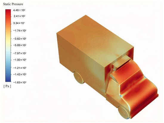
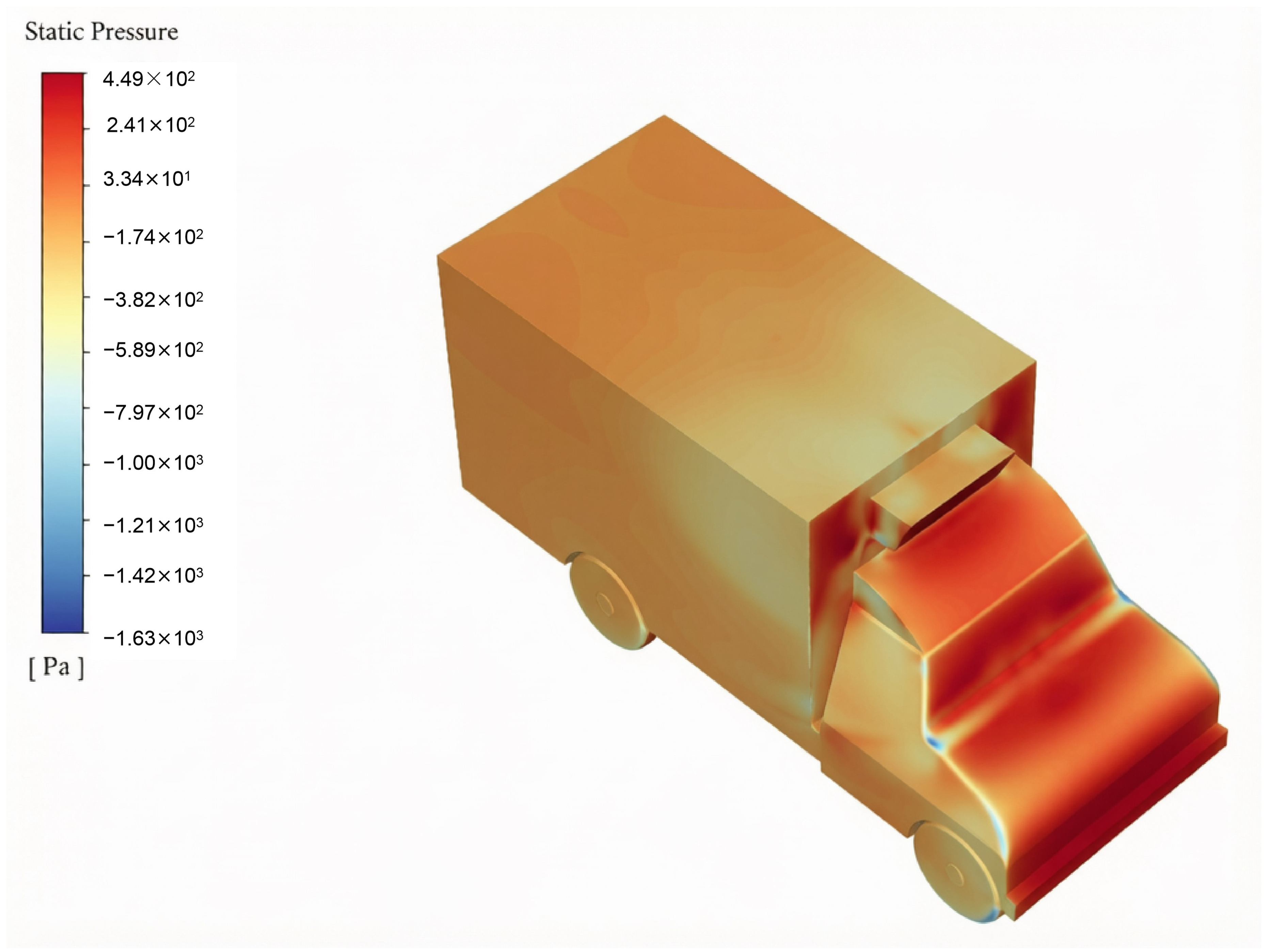
Figure 13 presents the pressure distribution of the model at 90 km/h. After installation of the flow deflector, a gradual pressure-recovery region formed along the deflector and the front edge of the cargo compartment, which is consistent with the reduced velocity gradient and smaller separation region. A directly paired baseline pressure contour was not available; this is acknowledged as a limitation in Section 4.3.

Figure 13. Pressure distribution diagram of the model with a flow deflector installed.

Air resistance has a significant influence on vehicle traveling performance. A lower drag coefficient indicates that the vehicle is less affected by air resistance at high speeds, whereas a higher drag coefficient results in greater resistance at high speeds. Therefore, a lower drag coefficient is more favorable. A vector perpendicular to the ground was selected for force calculation, and the resulting value represents the down force acting on the vehicle, reflecting the vehicle’s ability to achieve better handling performance during traveling. The calculated resistance acting on the overall vehicle components at different traveling speeds is presented in Table 6. Such phenomenon may be due to the flow deflector deflecting airflow, accelerating it above the roof and creating a low-pressure zone beneath. According to Bernoulli’s principle, this pressure difference between the top and bottom generates additional downforce.

Table 6. Total down force of two models at different traveling speeds.

Model	50 km/h	70 km/h	90 km/h
Initial model	46.75/N	93.45/N	111.37/N
Model with a flow deflector installed	72.74/N	121.37/N	220.07/N

The drag coefficient is one of the indicators used to evaluate overall vehicle performance. Using the fixed reference area A = 4.12 m², the drag coefficient decreased by 14.0%, 14.4%, and 15.0% at 50, 70, and 90 km/h, respectively, as shown in Table 7. Thus, the benefit of the flow deflector increased slightly with vehicle speed.

Table 7. Comparison of the effect after the installation of the flow deflector.

Traveling Speed/(km/h)	Driving Resistance Fw/N		Drag Coefficient Cd
	Original Model	Model with a Flow Deflector Installed	Original Model	Model with a Flow Deflector Installed
50	392.83	337.77	0.807	0.693
70	705.50	604.16	0.740	0.633
90	1113.74	946.41	0.706	0.599

The aerodynamic benefit observed here is consistent with the separation-control principle reported for cab-roof fairings, front deflectors, and gap-control devices. In this study, only the deflector was changed while the vehicle geometry, computational domain, mesh, reference area, and boundary conditions were kept constant. This paired comparison isolates the structural effect of the proposed deflector. The drag coefficient decreased by 14.0%, 14.4%, and 15.0% at 50, 70, and 90 km/h, respectively. The corresponding flow fields show a weaker velocity gradient and reduced separation at the front edge of the cargo compartment. Compared with full-height roof fairings or gap-closing devices, the present thin-walled deflector achieves a consistent aerodynamic improvement with a compact structure that does not alter the cab-to-cargo gap. These results support the structural effectiveness of the proposed design for the target refrigerated-truck geometry, while the absolute drag values remain specific to this configuration.

4.3. Limitations and Future Work

The maximum tested speed of 90 km/h reflects the upper end of the operating range considered for urban and regional refrigerated-truck distribution; it was not imposed by a technical limitation of the PIV system. Higher speeds may occur in long-haul refrigerated transport and will be considered in future work.

The geometry was simplified, wheel rotation was neglected, and the rearview mirrors and underhood components were removed. These choices are consistent with previous simplified truck studies and were verified through the front-body PIV comparison, but absolute wake-related drag may differ from road conditions.

The PIV measurements were limited to the front-body approach region and do not fully validate the rear wake. The low-speed scaled model also cannot reproduce the full-scale Reynolds number, and no blockage correction was applied because the study focused on the relative change in front-body resistance rather than absolute wake quantities.

A formal three-grid GCI study and a stored y+ contour were not available in the original dataset. The reported mesh quality and near-wall treatment therefore support, but do not replace, a full grid-independence study [31].

Only the presence or absence of the flow deflector and vehicle speed were varied. Future work will optimize the deflector angle, height, position, and curvature and will include rotating wheels and a broader PIV measurement plane.

5. Conclusions

In this study, a refrigerated-truck traveling model was established using numerical simulation, and the driving resistance characteristics of the refrigerated truck after the installation of a flow deflector were investigated.

By setting the corresponding boundary conditions and solver parameters, the external flow field of the model was numerically solved to simulate the resistance characteristics under different operating conditions, and the reliability of the model was validated using PIV measurements. The results of this study can provide support for reducing the aerodynamic resistance and energy consumption of relevant vehicles. The main conclusions are as follows.

(1)

In the absence of a flow deflector, the lack of a streamlined design and the structural constraints imposed by the cargo compartment and the roof-mounted unit caused an abrupt change in the velocity gradient in the front region of the cargo compartment, where significant flow separation occurred, thereby resulting in poor overall aerodynamic performance.

(2)

After the flow deflector was installed, the continuity of the flow field at the front of the vehicle was improved and the aerodynamic resistance was reduced. At 90 km/h, the air resistance decreased from 1159.55 N to 985.34 N and the drag coefficient decreased from 0.735 to 0.624, corresponding to a reduction of 15.0%. Across the tested range of 50–90 km/h, the drag-coefficient reduction was 14.0–15.0%.

By constructing the PIV experimental platform and measuring the velocity field in the front-body region, the mean relative error between the PIV and CFD velocities was found to be 4.72%, with a standard deviation of 1.63%. This result supports the reliability and feasibility of the model within the measured region, although it does not constitute a full validation of the rear wake.

It is worth noting that the shape and dimensional parameters of the flow deflector may affect the research results to some extent. Further research on these parameters will be conducted in subsequent studies.

References

- Wang, Y.; Xie, H.X.; Gou, M.Y.; Zhao, X.Q. Fresh Commodity Multi-compartment Loading Distribution Routing Optimization Problem Based on Vehicle Sharing. Packag. Eng. 2025, 46, 210–220. (In Chinese) [Google Scholar]
- Fan, R.W.; Chen, X.D.; Wang, Q.W.; Tan, W.Y.; Fan, P.Y.; Wang, S.; Wu, Q.H. Research on Aerodynamic Braking System for High-speed Trains. Locomot. Car 2026, 46, 30–35. (In Chinese) [Google Scholar]
- Connolly, M.G.; Ivankovic, A.; O’Rourke, M.J. Drag reduction technology and devices for road vehicles-A comprehensive review. Heliyon 2024, 10, e33757. [Google Scholar] [CrossRef] [Scilit] [PubMed]
- Levin, J.; Chen, S.H. Aerodynamic of a refrigerated truck and improvement to reduce its aerodynamic drag. Proc. Inst. Mech. Eng. Part D J. Automob. Eng. 2023, 237, 2527–2538. [Google Scholar] [CrossRef] [Scilit]
- Suntaxi, V.G.S.; García, A.C.; Ávila Rondón, R.L. CFD-Based Assessment of the Aerodynamic Influence of a Front Deflector on Drag, Lift, and Propulsion Power in a Medium-Duty Freight Truck. Vehicles 2026, 8, 167. [Google Scholar] [CrossRef] [Scilit]
- Charles, T.; Yang, Z. Comparison of the effectiveness of drag reduction devices on a simplified truck model through numerical simulation. Modelling 2022, 3, 300–313. [Google Scholar] [CrossRef] [Scilit]
- Yuan, Z.; Xiang, W.; Zhang, H.; Zhao, Z. Optimisation study of aerodynamic drag based on flow field topology in box-type trucks. Int. J. Veh. Perform. 2024, 10, 96–118. [Google Scholar] [CrossRef] [Scilit]
- Seyhan, M.; Es, H.A.; Sarioglu, M. Optimization of aerodynamic drag reduction for truck trailer model via machine learning. Measurement 2025, 240, 115604. [Google Scholar] [CrossRef] [Scilit]
- Bardera, R.; Matías-García, J.C.; Barroso-Barderas, E.; Fernández-Antón, J.; Rodríguez-Sevillano, A.A. Active Flow Control by Coanda Actuators for Aerodynamic Drag Reduction in a European-Type Truck. Actuators 2025, 14, 556. [Google Scholar] [CrossRef] [Scilit]
- Wright, C.; Al-Rawi, M. One-way fluid structure interaction of a utility vehicle splitter using CFD modelling. CFD Lett. 2023, 15, 34–43. [Google Scholar] [CrossRef] [Scilit]
- Kim, S.H.; Kim, J.J. Experimental investigation of aerodynamic drag reduction in a light commercial vehicle using cab extenders. Int. J. Heat Fluid Flow 2026, 120, 110392. [Google Scholar] [CrossRef] [Scilit]
- Lu, Y.; Fu, S.; Li, L.Z. Simulation of Optimal Layout of Jet Fans in Large Rectangular Sectional Underwater Tunnel. J. Highw. Transp. Res. Dev. 2021, 38, 81–86. (In Chinese) [Google Scholar] [CrossRef]
- Yan, Z.; Fan, Q.; Zhang, Q.; Xu, L. Numerical and experimental investigation of bionic fairing for hydrodynamic performance optimization in amphibious unmanned platforms. Ocean Eng. 2026, 349, 124049. [Google Scholar] [CrossRef] [Scilit]
- Hu, Z.W.; Wu, Q.J.; Liu, X.C.; Jin, X.Z.; Zhou, L.; He, Z.G.; Luo, X. Comparative Analysis of Outflow Field of Van Guide Cowl. Automob. Appl. Technol. 2020, 45, 21–23. (In Chinese) [Google Scholar] [CrossRef]
- Lin, C.B.; Xu, E.Y.; Feng, G.S.; Zhan, X. Vehicle External Flow Analysis and Optimization for Commercial Vehicle. Equip. Manuf. Technol. 2018, 1, 18–21. (In Chinese) [Google Scholar] [CrossRef]
- Zhang, J.Z.; Ma, Z.Q. Simulation study based on vehicle drag optimization and flow deflector development. Auto Time 2020, 128–129, 148. (In Chinese) [Google Scholar]
- Zhao, L.S.; Du, G.S. Experimental Study on Reducing Aerodynamic Resistance of Vans with Cover in a Wind Tunnel. Trans. Chin. Soc. Agric. Mach. 2000, 31, 67–69. (In Chinese) [Google Scholar] [CrossRef]
- Zhang, J.; Ding, Y.S.; Deng, H.; Han, S.; Gao, G.J. Effect of pantograph bionic deflectors on aerodynamic performance of high-speed under crosswind. J. Railw. Sci. Eng. 2024, 21, 936–948. (In Chinese) [Google Scholar] [CrossRef]
- Yang, W.; Yue, H.; Deng, E.; He, X.; Zou, Y.; Wang, Y. Comparison of aerodynamic performance of high-speed train driving on tunnel-bridge section under fluctuating winds based on three turbulence models. J. Wind Eng. Ind. Aerodyn. 2022, 228, 105081. [Google Scholar] [CrossRef] [Scilit]
- Karimi, M.; Akdogan, G.; Bradshaw, S.M. Effects of different mesh schemes and turbulence models in cfd modelling of stirred tanks. Physicochem. Probl. Miner. Process. 2012, 48, 513–531. [Google Scholar] [CrossRef]
- Roache, P.J. Perspective: A method for uniform reporting of grid refinement studies. J. Fluids Eng. 1994, 116, 405–413. [Google Scholar] [CrossRef] [Scilit]
- Wu, H.W.; Su, C.Q.; Wang, Y.P.; Liu, X. Research on Fuel Economy of Platooning Cars Under Crosswind Condition. J. Wuhan Univ. Technol. 2023, 45, 53–62. (In Chinese) [Google Scholar]
- Menter, F.R. Two-equation eddy-viscosity turbulence models for engineering applications. AIAA J. 1994, 32, 1598–1605. [Google Scholar] [CrossRef] [Scilit] [PubMed]
- Hamilton, D.; Sessions, J.; Langevin, C. Identifying rolling resistance and air resistance simultaneously for an electric truck. Int. J. For. Eng. 2026, 37, 225–239. [Google Scholar] [CrossRef] [Scilit]
- Mohamed-Kassim, Z.; Filippone, A. Fuel savings on a heavy vehicle via aerodynamic drag reduction. Transp. Res. Part D Transp. Environ. 2010, 15, 275–284. [Google Scholar] [CrossRef] [Scilit]
- Zheng, G.S.; Guan, R.Q.; Feng, X.M.; Liu, C.Q.; Ge, N. Numerical Simulation and Experimental Research for Plane Cascade of Variable Geometry Turbine. Mach. Build. Autom. 2023, 52, 141–144. (In Chinese) [Google Scholar]
- Li, D.C.; Liu, Y.L.; Kan, Z.; Li, Y.K.; Kong, L.Q.; Lu, Y.X. Review of low-altitude aerodynamic environments and their effects on UAV aerodynamics. J. Natl. Univ. Def. Technol. 2026, 48, 1–28. (In Chinese) [Google Scholar]
- Zhang, Y.; Liu, S.Y.; Li, J.J.; Zhang, C.; Wang, X.F. PIV Measurement and Numerical Investigation of Three-dimensional Velocity Field sround Wind Turbine Blades. J. Eng. Thermophys. 2022, 43, 2642–2646. (In Chinese) [Google Scholar]
- Hüttig, S.; Kühn, M.; Gericke, T.; Bloem, G.; Sciacchitano, A.; Akkermans, R.A.D. On-road vehicle aerodynamics with a large-scale stereoscopic-PIV setup: “the Ring of Fire”. Exp. Fluids 2025, 66, 125. [Google Scholar] [CrossRef] [Scilit]
- Ferhath, A.A. Advanced approaches to flow visualisation techniques for vehicle damper performance and safety enhancement. Discov. Mech. Eng. 2025, 4, 48. [Google Scholar] [CrossRef] [Scilit]
- Celik, I.B.; Ghia, U.; Roache, P.J.; Freitas, C.J. Procedure for estimation and reporting of uncertainty due to discretization in CFD applications. J. Fluids Eng. 2008, 130, 078001. [Google Scholar] [CrossRef] [Scilit]
Disclaimer/Publisher’s Note: The statements, opinions and data contained in all publications are solely those of the individual author(s) and contributor(s) and not of MDPI and/or the editor(s). MDPI and/or the editor(s) disclaim responsibility for any injury to people or property resulting from any ideas, methods, instructions or products referred to in the content. |
© 2026 by the authors. Licensee MDPI, Basel, Switzerland. This article is an open access article distributed under the terms and conditions of the Creative Commons Attribution (CC BY) license.