


Abstract
Electric vertical take-off and landing (eVTOL) aircrafts are emerging as the core enabler of urban air mobility (UAM), and their safe and efficient energy management relies on accurate knowledge of the battery power load. Existing research has focused on battery state estimation or mission-level energy modeling, leaving the second-level power demand of disturbed flight essentially unpredicted. This paper proposes a four-dimensional (4D) trajectory-based framework for eVTOL battery power forecasting. A physics-based power model first translates 4D trajectories into reference power profiles; multi-factor perturbations—three-dimensional wind, temperature, and mass—are then applied under emulated closed-loop flight control, yielding a trajectory–power database of 1,047,970 samples from 1000 simulated missions of the certified EHang 216-S multirotor, whose reference mission stays inside the certified envelope of 200 m above ground level, 30 km, and 25 min. A two-layer long short-term memory (LSTM) network maps a 10 s window of trajectory and power history, together with the flight phase and the distance remaining to the next phase boundary, to the battery power over the next 5 s. On the held-out test set it attains a root-mean-square error (RMSE) of 3.483 kW—50.9% below the physics baseline (7.089 kW) and 16.9% below a linear predictor given exactly the same inputs—with the residual tail dominated by flight-phase transitions. Ablations show that the power-history input channel is decisive, whereas network depth and residual connections matter little; extending the horizon to 10 and 15 s preserves 39.6% and 33.5% error reductions, with sub-linear growth. The framework combines physical interpretability with data-driven adaptability, offering a prospective forecasting capability for the battery management systems of electric aircraft.
1. Introduction
The low-altitude economy is emerging as a strategic industry: in China, its market reached approximately 506 billion CNY in 2023 and is projected to approach two trillion CNY by 2030 [1]. Among low-altitude aircraft, electric vertical take-off and landing (eVTOL) vehicles have moved from concept demonstrations to initial commercial operations, led by type-certified multirotor products. Their power battery is a principal bottleneck: current lithium-ion energy density constrains range and payload [2,3]; the eVTOL duty cycle—repeated high-rate discharge at take-off and landing superimposed on a sustained cruise load—differs fundamentally from automotive usage and accelerates aging [3,4]; and the safety consequences of a power shortfall in flight are far more severe than on the ground [5]. Knowing the near-future battery power load seconds ahead, under the disturbances an aircraft actually meets, is, therefore, valuable at the design stage (cell selection, pack sizing, power-margin, and thermal design) and indispensable in operation, where predictive battery management, power-margin monitoring, and the fleet-level demand estimates underlying urban air mobility (UAM)–grid interaction all consume short-horizon load forecasts [6,7]. System-level studies of this aircraft class have addressed the feasibility of current and emerging battery chemistries [8] and the architecture of the flight-control actuation system [9].
The first research gap is one of resolution and conditions. Physics-based eVTOL energy models are relatively mature and quantitatively verified, but at mission scale and under nominal conditions. The sizing and mission-analysis framework of Yanev and Staack reproduces mission energy within approximately 10% [10], detailed power-consumption models support low-altitude UAM mission studies [11], and comparative powertrain analyses balance energy over complete missions [6,7]. What such models imply at the second-level resolution that governs battery stress has remained unquantified, and the answer turns out to be severe: evaluated at 1 Hz under moderate turbulence, an idealized physics model of this same form errs by 7.089 kW, about 16% of the mean disturbed cruise demand (Section 4.2). Optimization-based work has addressed four-dimensional trajectory design under critical-engine-inoperative constraints [12] and surrogate-based take-off trajectory design for electric drones [13].
The second gap is one of quantity and coupling. Learning-based prediction has achieved high accuracy in adjacent domains, but with different quantities. Selje et al. benchmarked machine-learning techniques for flight-level energy consumption in advanced air mobility [14]. For electric buses, a transformer model predicts the energy consumption rate over 250 m to 10 km look-ahead distances with mean absolute errors decreasing from 0.28 to 0.09 kWh/km [15]—an energy-per-distance measure aggregated over minutes, not the instantaneous power at second-level resolution. Four-dimensional (4D) trajectory prediction, though advancing rapidly [16], forecasts future positions rather than power, and therefore cannot exploit the coupling between trajectory, atmospheric disturbance, and the battery load that physically generates the load fluctuations. The missing quantity is, meanwhile, exactly what fleet-level studies presuppose: joint eVTOL scheduling under dynamic demand [17] and the integrated optimization of eVTOL fleets with power systems [18] both require short-horizon vehicle load forecasts that current methods struggle to provide faithfully. For eVTOL specifically, transfer-learning-enhanced generative models have been used to predict take-off trajectories [19].
Operational eVTOL power data are scarce—certified fleets are small, telemetry is proprietary, and no public dataset offers second-level power records under atmospheric disturbances—so this paper closes these gaps by using a simulation: a study of eVTOL battery power prediction from 4D trajectory data. The task is defined at second-level resolution: given the most recent 10 s of the 4D trajectory and power history, together with the flight phase and the distance remaining to the next phase boundary, predict the battery output power over the next 5 s. A simulation platform built around the certified EHang 216-S multirotor provides 1,047,970 supervised samples from 1000 trajectories, on which a two-layer long short-term memory (LSTM) network is compared with model-based, statistical, and linear baselines on a trajectory-level held-out test set. The contributions, and their quantified increments, are threefold: (i) a single power model that both generates the training data and serves as the physics baseline, so that the baseline error (7.089 kW root-mean-square error, RMSE) isolates genuine disturbance effects rather than model-form mismatch and is reduced by the learned predictor to 3.483 kW, a 50.9% reduction; (ii) a physics-informed input design—4D trajectory, power history, phase encoding, and the distance remaining to the next phase boundary—whose decisive channels are identified ablatively (masking the power history degrades the RMSE by a factor of 1.67, to the level of persistence), together with a depth sweep showing that a shallow plain model is sufficient and that the residual variant is equivalent to the plain model under a matched dropout rate and training budget; and (iii) a disturbance emulation, reproducing realistic short-term power fluctuations (a cruise-phase 5th–95th percentile range of 33.9–54.4 kW over the 1000-trajectory ensemble against the 40.0 kW nominal).
2. Materials and Methods
2.1. Overall Framework and Problem Formulation
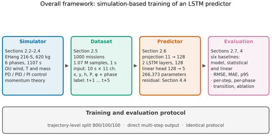
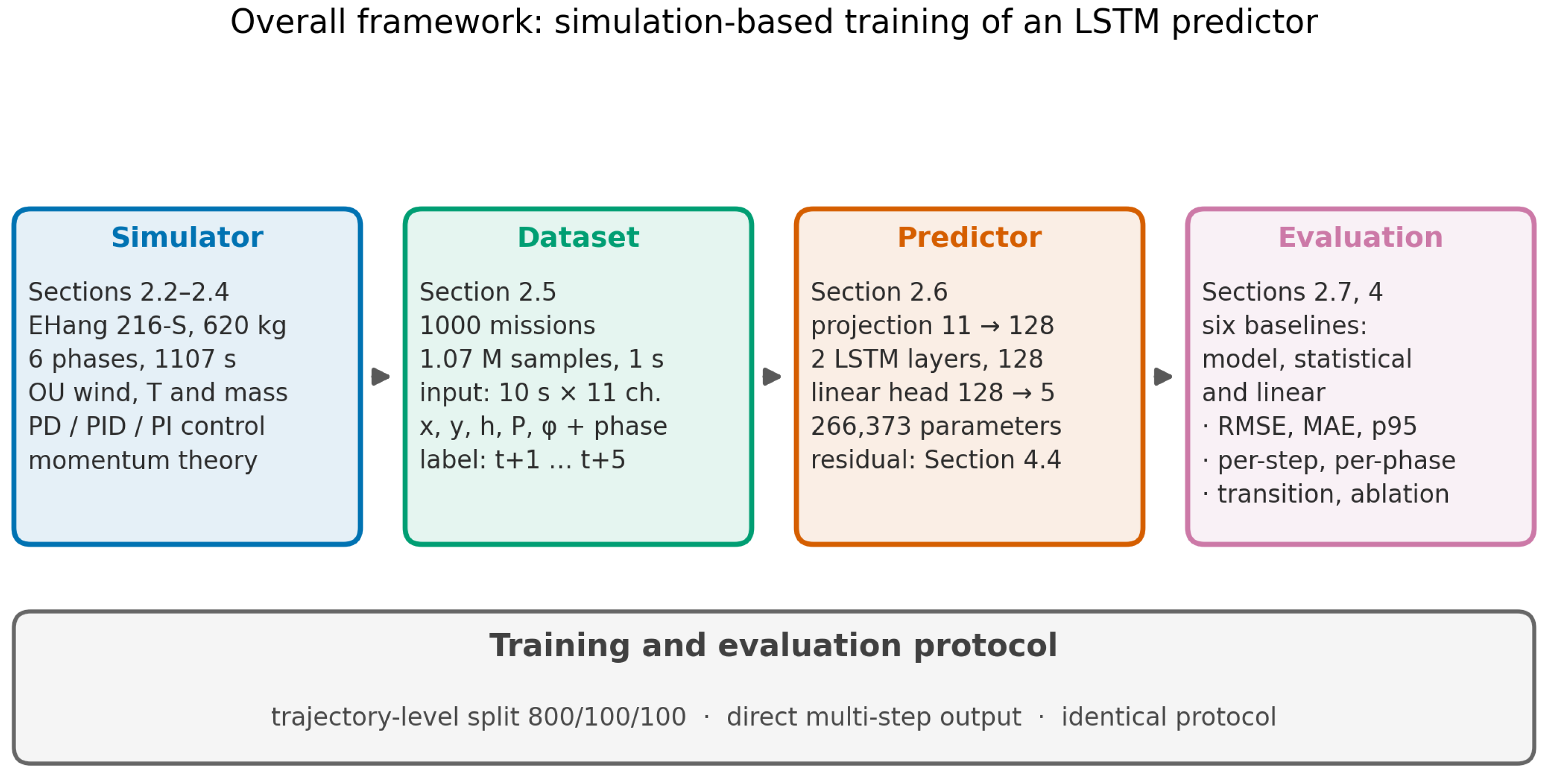
Figure 1 illustrates the overall framework: a simulation platform generates realistic 4D flight trajectories under stochastic atmospheric disturbances and emulated flight control; a sliding-window scheme constructs the supervised dataset; and an LSTM network trained on the recent trajectory and power history is evaluated against model-based, statistical, and naive baselines on an independent test set.
Figure 1.
The overall framework of the study: simulation-based training and the evaluation of an LSTM battery-power predictor.
Let , ri = (ti, xi, yi, hi) denote a 4D trajectory sampled at a uniform interval Δt, with x, y, and h the along-track, cross-track, and vertical coordinates; let Pi be the battery output power and ci ∈ {1,…,6} the flight-phase index. The prediction task is as follows: given the most recent L seconds of trajectory and power history, predict the battery power over the next H seconds:
where Δxj = xj − xt−L+1 is the window-relative along-track displacement and e(cj) ∈ {0,1}6 the phase one-hot encoding. The along-track coordinate is window-relative because the cruise phase is translation-invariant along the track. Critically, the aerodynamic power of a multirotor is governed by the airspeed rather than the groundspeed (Section 2.4); since wind is unobservable from position records, the power history Pj is included so that the network can implicitly infer the prevailing disturbance state from the power response it induces. In addition, a fifth physical channel is included: the remaining distance to the next phase-trigger boundary expressed as a fraction of the span of the active phase (denoted φ). Because the along-track coordinate is window-relative, a position-triggered boundary would otherwise be invisible to the network until it had been crossed; the boundary positions follow from the pre-loaded flight plan and the current position is available on board, so this quantity is directly observable.
2.2. Simulation Platform
2.2.1. Aircraft Model
The simulated aircraft is a pure multirotor with Nr rotors of the diameter Dp (total disk area A = Nrπ(Dp/2)2). The frontal area Af is the cross-section of the smallest sphere enclosing the airframe, with the drag coefficient Cd [20]; the propulsive efficiency η lumps motor, controller, and rotor losses into one factor [20]; and the auxiliary power Paux bounds the total demand from below.
2.2.2. Reference Flight Profile
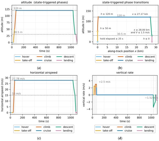
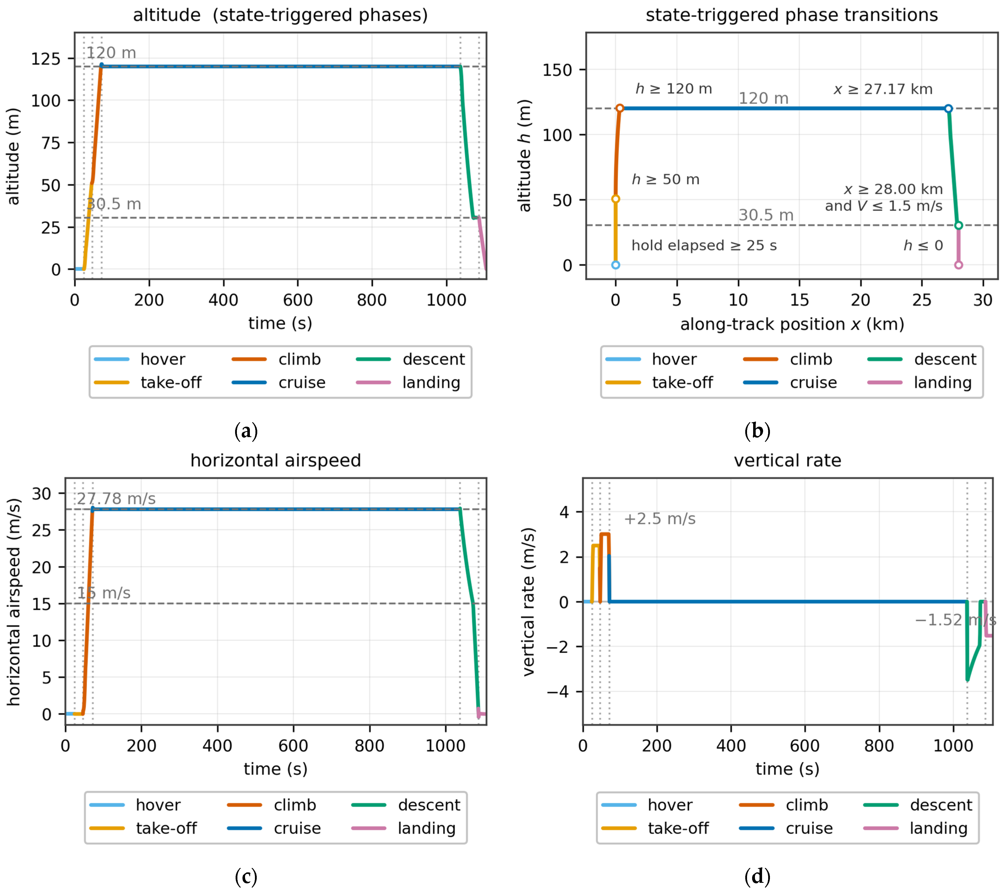
A six-phase reference profile emulates an urban air mobility mission. The aircraft modeled here is certified to execute a pre-loaded flight plan automatically [21], so the profile is implemented as a flight program rather than as a time schedule: apart from the initial hold, every transition fires when the aircraft reaches a prescribed altitude, along-track position, or airspeed, and each boundary is, therefore, an event an on-board system can observe directly. The remaining distance to the next boundary is thus available on board and is supplied to the predictor as a fifth input channel (Section 2.1). A 25 s pre-departure hold precedes a vertical take-off to 50 m at 2.5 m/s; the climb to the 120 m cruise altitude at 3.0 m/s accelerates the airspeed to 27.78 m/s; cruise is held until the aircraft reaches the top-of-descent position derived from the approach geometry; and the approach then follows a constant 12.5% (7.13°) glide slope from 120 m to a 30.5 m level-off altitude while decelerating to 15 m/s, decelerates to zero in level flight, and a final vertical descent at 1.52 m/s completes the mission.
The segment geometry and rates are design choices anchored to published practice rather than prescribed by any standard: the slope figures that appear in vertiport and heliport regulation are obstacle-limitation surfaces, not flown trajectories, as the source table itself states [22], and the applicable certification means of compliance leaves the flown approach path to the applicant [23]. The 12.5% (7.13°) glide slope is compatible with the 8:1 approach surface of the FAA Engineering Brief (EB) 105A [24] and with the category-C slope of the obstacle-limitation surfaces in the EASA Notice of Proposed Amendment (NPA) 2026-01 [22], and it does not exceed the 12.5% limit adopted in the VFR vertiport procedure of Kim et al. [25]. The 30.5 m level-off altitude is the high-hover height of the EASA MOC-2 (Means of Compliance) SC-VTOL [23], and the 50 m take-off height is a design choice within the published range of terminal-area level-off altitudes, which extends from 30.5 m [23] to the 200 m level leg from which Qanbari and Skorupski fly their vertical descent [26]. The vertical rates of 2.5 m/s for the take-off and 3.0 m/s for the climb are those adopted for vertiport terminal-area operations by Song [27], and the 1.52 m/s final descent is the −300 ft/min applied to the eVTOL descent segments of Clarke and Alonso [28]. The terminal structure—level deceleration, followed by a pure vertical descent—is a geometric necessity rather than a stylistic choice: because the vertical rate on a constant-slope glide is the slope times the ground speed, an aircraft that decelerated to zero on the glide itself would never reach the pad. The same structure appears as the constant-altitude terminal segments of Clarke and Alonso [28], as the 135 m level leg followed by a 200 m vertical descent of Qanbari and Skorupski [26], and as the operational rule that vertical speed is reduced to zero before the aircraft descends below the landing screen height [29]. The approach-end speed of 15 m/s follows from requiring the descent rate to stay inside the published band of 1.5–3.0 m/s [27,28] at the fixed 12.5% slope for the final approach speed of 15 m/s used here (1.88 m/s), which admits 12–24 m/s; the level deceleration rate of 1.0 m/s2 is a design choice well inside the longitudinal and vertical acceleration limits assumed for passenger comfort from Beyne and Castro [29]. Within the take-off, climb, and landing segments, the vertical reference is rate-limited at 1.0 m/s2, so those references carry no velocity step; the position-scheduled glide is shaped by the same limiter where its vertical rate changes, at the top of descent, at the level-off, and at the handover to the vertical descent.
2.2.3. Atmospheric Disturbances
The air density follows an exponential approximation of the International Standard Atmosphere with a trajectory-specific temperature offset δT [30]:
and the take-off mass is randomized as m = m0ξm to emulate variations in payloads and loading conditions. The three-dimensional wind field is the superposition of two Ornstein–Uhlenbeck (OU) processes per axis—a slow component (τs, σs), representing synoptic-scale gusts, and a fast component (τf, σf), representing small-scale turbulence—discretized in steady-state-variance-preserving form and bounded by a smooth saturation:
where εi∼N(0,1) and wmax have separate horizontal and vertical limits (Section 3.2).
2.2.4. Numerical Implementation and Reproducibility
All time-varying elements of the platform are advanced at a fixed step Δt = 1 s, matching an assumed 1 Hz sensing and control update rate: the OU wind of Equation (3) is advanced directly in the steady-state-variance-preserving form shown there, the control laws in Section 2.3 are inherently discrete (sampled-data operation at 1 Hz), and the dynamics that are explicitly integrated—the airspeed response and the trajectory kinematics—use the explicit (forward) Euler scheme. The 1 s step is small against the governing time constant of the integrated dynamics (the 3 s airspeed lag), and the tracking errors are bounded by the emulated controller rather than by numerical stabilization. The simulator is implemented in Python 3.10 with NumPy 2.2.6; trajectory i is generated with the independent random generator np.random.default_rng(42 + i), so that every trajectory—and hence the full dataset—is exactly reproducible from the settings reported in Section 3.
2.3. Flight Control Emulation
An eVTOL aircraft in operation must not deviate substantially from its cleared trajectory, so a three-channel control law emulating a pilot or autopilot is implemented: a proportional–derivative (PD) altitude channel, a proportional–integral–derivative (PID) cross-track channel (the derivative term being essential for sampled-data stability), and a proportional–integral (PI) along-track channel with an additional airspeed damper. With tracking errors defined as reference minus measurement (eh = h* − h, ey = −y, ex = x* − x), and error rates from first differences, , the raw corrective commands, their discrete filtering and saturation, and the airspeed response are implemented exactly as
where Ii is the integrator state with clamping ± Imax (anti-windup), β is the low-pass coefficient associated with the control bandwidth τp (finite actuation bandwidth), and the saturation limits of the corrective commands are sized to the maximum wind speeds the controller is allowed to counteract. All three channels are updated once per second in sampled-data fashion: commands are computed from the previous step’s measurements and enter the current step’s state update, synchronously with the trajectory integration in Section 2.2.4. A key decision is the explicit airspeed/groundspeed separation: the controller commands the airspeed Va, responding as a first-order system with a time constant τV, whereas the ground track integrates the groundspeed Vg = Va + wx —physically necessary because the aerodynamic power depends on the air-relative velocity while the trajectory evolves inertially. The commanded vertical rate is additionally limited in acceleration to 1.0 m/s2, the vertical-acceleration capability assumed here. The two vertical-velocity channels used by the power model in Section 2.4 are taken from the resolved reference and the integrated states without further low-pass filtering: because the reference rate is rate-limited, the differentiated signal is already smooth, and filtering it would only delay the response to genuine changes in vertical rate. The resulting corrective actions induce the realistic short-term power fluctuations that an open-loop simulation would not produce.
Ii = clip(Ii−1 + eiΔt,±Imax),
2.4. Battery Power Model
The battery power is evaluated by a unified physics model invoked identically for the reference and every disturbed trajectory—only the input states differ—so the baseline error in Section 4 reflects genuine disturbance effects, not model–form inconsistency. As the aircraft is wingless and fully rotor-powered, the model is built on classical momentum theory [31], which relates the thrust FT of a rotor to the induced velocity vi at the disk through the implicit equation
where U is the free-stream speed in the plane of the disc. Squaring Equation (13) and defining the hover-induced velocity yields a biquadratic in vi, , whose unique positive root is the closed form used for the forward-flight relations below—no iterative solution is required. Vertical flight is governed instead by the axial momentum balance, whose positive root is the induced velocity; for a climb rate vc, the induced velocity and shaft power of a rotor at thrust FT are
and for forward flight at airspeed Va, the corresponding closed forms are
The parasite term scales with , so a headwind or tailwind |wx| shifts the cruise parasite power by roughly ; this cubic sensitivity is the principal mechanism by which atmospheric disturbances invalidate the physics baseline.
Two simplifications in the parasite term should be stated explicitly. First, the frontal reference area Af is defined geometrically, as the cross-section of the smallest sphere enclosing the airframe; it is a reference area rather than a measured aerodynamic projection, and Cd is correspondingly a lumped coefficient. The quantity that enters the power balance is, therefore, the product CdAf, which is 1.131 m2 and lies within the range reported for multirotor airframes of this class; the two factors are not separately identifiable from the available data and should be interpreted jointly. Second, the model assumes a single orientation-independent drag coefficient: the dependence of parasite drag on the angle of attack and sideslip is neglected. For a wingless, fully rotor-powered configuration, the frontal projection varies little across the flight envelope, so this dependence is weak; the simplification is made for computational tractability, and replacing the lumped term with an aerodynamic model whose drag coefficient depends on angle of attack and sideslip, calibrated against wind-tunnel or higher-fidelity CFD data, is identified as future work in Section 4.5.
Maneuvering and unsteady effects complete the power balance. The effective rotor thrust combines the weight with the acceleration loads, with W = mg, and the lateral load factor is . Wingless forward flight adds the potential-energy term Pgrav = Wvc,g/η and the non-negative acceleration power Pacc = max(WaaVa/g,0)/η. Two distinct vertical velocities enter the balance. The axial momentum relations (Equations (14)–(16)) apply to hover, take-off, climb, and landing, and use the air-mass-relative climb rate , whereas the forward-flight forms (17) and (18), which apply to cruise and descent, are evaluated at the level-flight induced velocity and, therefore, carry no axial-rate dependence; the frame-invariant potential-energy term of those phases uses the inertial rate . In descent, Pgrav is negative; since no regenerative recovery is assumed, the total power is floored at Paux.
The rotor model is a momentum-theory actuator disk and, therefore, carries no blade geometry: the periodicity of the local blade loading that arises in edgewise flight, where the advancing and retreating sides of the disk see different relative flow speeds, is not resolved. All rotor losses beyond the ideal induced power—profile drag, the periodic-loading penalty, and the interference between the two rotors of each coaxial pair, which is a defining feature of the sixteen-rotor configuration used here—are lumped into the single propulsive efficiency, which is, therefore, an effective coefficient calibrated for this aircraft class, rather than a blade-resolved efficiency. Resolving blade-level aerodynamics, and, in particular, calibrating the coaxial interference penalty against flight-test or wind-tunnel data, is identified as future work in Section 4.5.
2.5. Dataset Construction
Trajectories are generated with per-trajectory random seeds, each with independently sampled wind, temperature, and mass. Supervised samples follow Equation (1): the input tensor Xt ∈ RL×11 stacks five physical channels (Δx, y, h, P, φ) and six one-hot phase channels over the L history steps, and the label is yt = (Pt+1,⋯, Pt+H). The L input steps must lie within a single phase; the H label steps may cross a phase boundary, and such samples are flagged as transition samples and analyzed separately in Section 4.3. To prevent leakage between strongly autocorrelated windows, the data are partitioned at the trajectory level, and all channels are standardized (z-score) with training-set statistics only.
2.6. LSTM Prediction Model
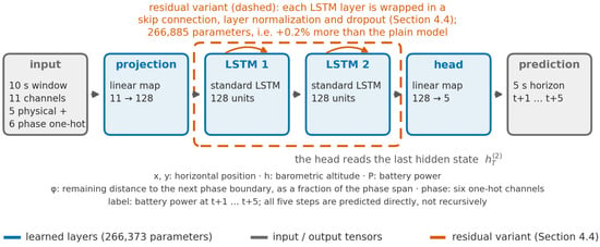
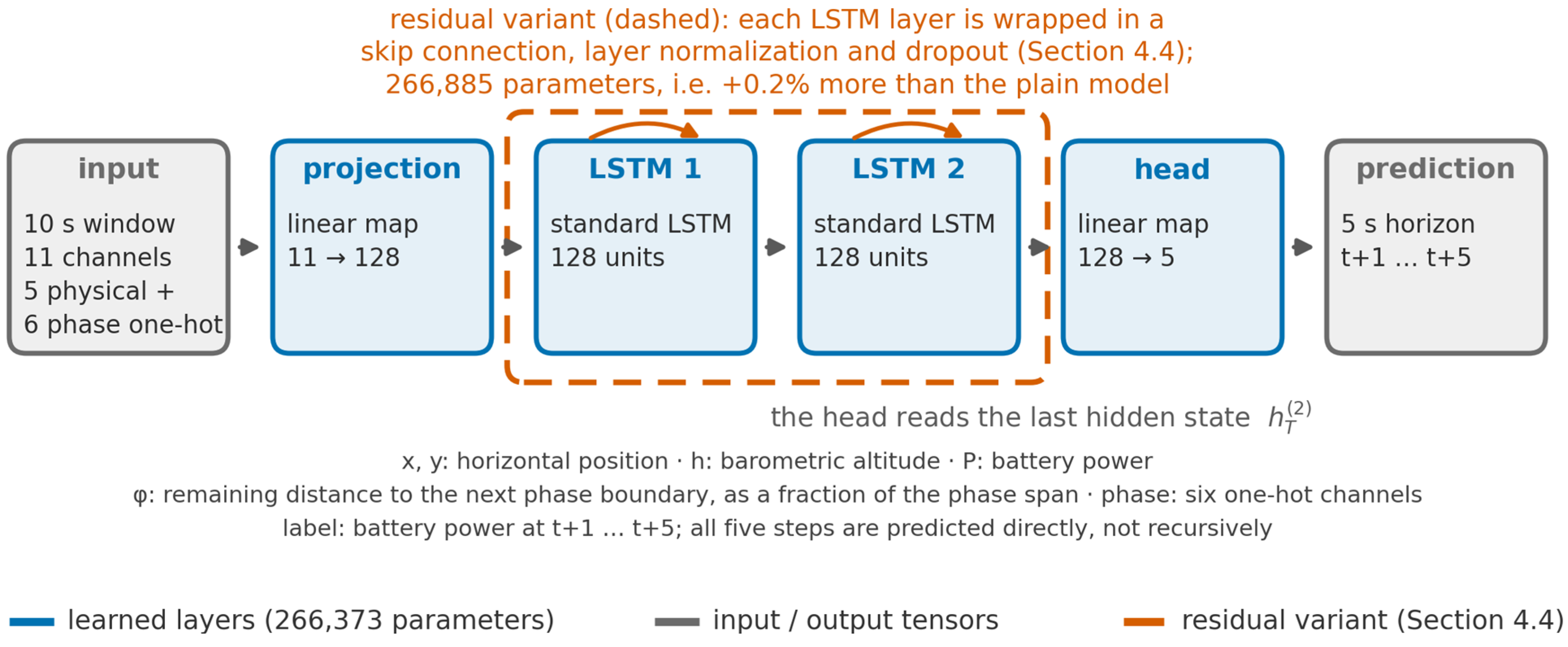
The predictor fθ (Figure 2) consists of a linear input projection to a d-dimensional space, two stacked standard LSTM layers [32], and a linear head that maps the last hidden state of the second layer to the H-step prediction. To test whether residual regularization benefits this task, a residual variant wraps each LSTM layer in a residual connection [33] with layer normalization [34] and dropout [35]; the variant adds only 0.2% more parameters, so any performance difference reflects the architecture rather than capacity. Training minimizes the mean squared error over the H steps with the Adam optimizer [36]; the residual variant is trained under a longer schedule (150 epochs against 100) because it converges more slowly, and with a lower dropout rate (0.1 against 0.2); because both the schedule and the dropout rate differ, Section 4.4 reports the two families under a matched dropout rate and epoch budget. Both families are swept from one to four layers in Section 4.4, on whose basis the plain two-layer configuration is retained as the final predictor.
Figure 2.
The prediction network: the 10 s input window is mapped to the 5 s power forecast by a linear projection, two stacked LSTM layers, and a linear head; the residual variant (dashed; ablated in Section 4.4) adds a skip connection, layer normalization, and dropout around each layer.
All reported runs are exactly reproducible. Training is implemented in PyTorch 2.5.1 (CUDA 12.1) under Python 3.10 with NumPy 2.2.6, with the random seed fixed at 42 for both PyTorch and NumPy before any model construction or data shuffling. Optimization uses Adam [36] with an initial learning rate of 10−3 and a batch size of 8192; the learning rate is halved whenever the validation loss fails to improve for ten consecutive epochs (fifteen for the residual variant), and training stops after at most 100 epochs (150 for the residual variant), with the checkpoint with the lowest validation loss being retained. All models were trained on a single NVIDIA GeForce RTX 3070 Laptop GPU (8 GB); the compact model size (266,373 parameters) and the direct multi-step output keep the training cost modest at the reported scale.
The choice of a learned sequence model, rather than a moving-horizon estimator (MHE), a Kalman-type filter, or a physics-informed hybrid estimator, follows from what is observable in this framework. The dominant disturbance is the wind, and the wind is not a recorded channel: the inputs are the 4D trajectory, the battery power, and the distance remaining to the next phase boundary. Because the aerodynamic demand depends on airspeed rather than groundspeed (Section 2.4), the prevailing air-relative state has to be inferred from the power it induces rather than read directly from the recorded channels. Both MHE and Kalman-type approaches require a process model of the disturbance with assumed statistics, and the central empirical finding of this work is that no such model, as implemented here with a random-walk prior, is adequate: under moderate turbulence the idealized estimator errs by 7.089 kW (Section 4.2), which is 16% of the mean disturbed cruise demand.
The power-history channel is what makes the problem tractable, and the evidence is direct: masking that channel raises the overall RMSE from 3.483 kW to 5.815 kW, i.e., to the level of the persistence baseline (Section 4.4). The network, therefore, acts as a learned observer of the unmeasured air-relative state, inferring that state from the power response it induces rather than from a disturbance model. A physics-informed formulation, in which the network is constrained to a residual of the analytic model, is structurally unhelpful for the same reason: the mapping from trajectory to power is already known and is evaluated exactly by the model in Section 2.4, so what is unknown is the unobserved exogenous input, not the functional form.
The learned formulation is also directly deployable: inference over a ten-step window by a network with 266,373 parameters takes about 1.15 ms per sample on a desktop CPU and involves no iteration at run time, whereas MHE requires an optimization solve at every control instant, which, in the same comparison, took about 17 ms per sample. A learned estimator is consequently the appropriate instrument for this task; it is not proposed as a replacement for model-based state estimation in general, and Section 4.5 sets out the staged path towards such a model, from recalibration on flight-test telemetry through fine-tuning on operational recordings to a structured flight-test campaign.
2.7. Baselines and Evaluation Metrics
Six baselines benchmark the proposed model: the physics baseline predicts the future power using the reference profile P*(t) tabulated along the flight program’s progress variable and read at the disturbed trajectory’s own altitude (for the altitude-scheduled phases), along-track position (for the position-scheduled phases), or its airspeed (for the airspeed-scheduled phase), i.e., an onboard model-based estimator that knows the plan but receives no disturbance feedback; the stage-average baseline predicts the per-phase mean power of the training set; the persistence baseline repeats the most recent observed power over all H steps; a linear-trend baseline extrapolates a least-squares line fitted to the most recent window of observed power; and an AR(10)+phase ridge baseline is a linear autoregression on the same ten power lags augmented with the phase encoding. An equal-information ridge baseline is a linear predictor supplied with exactly the same input vector as the LSTM—the same input window of physical channels together with the phase encoding—with its regularization strength selected on the validation set. Performance is measured by the root-mean-square error (RMSE) and the mean absolute error (MAE):
reported overall, per prediction step, and per flight phase. The median, 95th-percentile, and maximum absolute error (MaxAE) characterize the error tail.
3. Case Study
3.1. Aircraft and Mission Profile
The case-study aircraft is modeled after the EHang 216-S, a certified pure-multirotor eVTOL aircraft with sixteen coaxially paired rotors (Table 1). The disk area is A = 28.27 m2; the frontal area of the enclosing sphere (radius 3 m) is Af = 28.27 m2, with Cd = 0.04 [20]; the propulsive efficiency is taken as η = 0.85 [20]; and Paux = 1.0 kW is estimated for this weight class. The aerodynamic core of the model is consistent with published figures for this aircraft: at the 620 kg nominal take-off mass used throughout this study (Table 1), the momentum-theory hover power is 57.0 kW and the ideal cruise power (induced plus parasite) is 34.0 kW, against the 54 kW and 36 kW tabulated for this class [37]. The published hover value refers to a 600 kg aircraft, and the Froude power scales as the 3/2 power of the mass, which alone accounts for 5.0 of the 5.5 percentage points; on a mass-matched basis, the two hover figures agree to 0.5%, while the cruise comparison is 5.6% lower. The assumed propulsive efficiency of 0.85 is more optimistic than the value of about 0.65 implied by the published pack-level cruise figure of 55 kW, so the simulated electrical demand at cruise is lower than that figure implies; calibrating the efficiency against measured data is identified as future work in Section 4.5.
Table 1.
Main parameters of the simulated eVTOL aircraft (EHang 216-S) [20].
A six-phase reference profile with an estimated duration of 1107 s and a ground range of 28.0 km emulates an urban air mobility mission (Table 2 and Figure 3). The mission lies inside the certified envelope of the aircraft: CAAC SC-21-002 limits the EH216-S to a 30 km range, 25 min endurance, and 200 m above ground level [21], against which the case study uses 28.0 km, 18.5 min, and a 120 m cruise altitude. Under the reference conditions (nominal mass, standard atmosphere, and no wind), the power model yields phase-average powers of 67.1 kW (hover), 76.1 kW (take-off), 78.9 kW (climb), 40.0 kW (cruise), 30.7 kW (descent), and 62.1 kW (landing); the peak reference power, 83.5 kW, is reached in the climb, and the mission consumes 13.0 kWh, 42% of the 31 kWh pack. Cruise accounts for 87% of the mission duration and 83% of its energy; its 40.0 kW is shared between the rotor-induced power and parasite drag, the induced term being the larger, which is characteristic of a wingless multirotor configuration. The largest single step in the reference power is the 18.8 kW drop at the climb-to-cruise boundary, where the aircraft levels off and the climb and potential-energy contributions vanish. The prediction difficulty of such samples is analyzed in Section 4.3.
Table 2.
Six-phase reference flight profile.
Figure 3.
The six-phase reference mission profile of the case study (Table 2): (a) the reference altitude; (b) the reference mission in the along-track/altitude plane, with the state event that terminates each phase marked at the state where it fires—the initial hover holds station at zero along-track displacement and, therefore, appears as the point at the origin; (c) horizontal airspeed; (d) the vertical rate. The take-off and landing are vertical, so the horizontal airspeed is zero there while the vertical rate is +2.5 and −1.52 m/s, respectively; and the airspeeds in (c) are horizontal throughout, and no altitude change is commanded during cruise.
In Table 2, the last column lists horizontal airspeeds only. Because the case-study aircraft is a pure multirotor, its take-off and landing are vertical: the horizontal airspeed is zero in the hover, take-off, and landing phases, while rotor thrust is used to change altitude at the vertical rates given alongside the altitude column. Forward acceleration takes place during the en-route climb, where the horizontal airspeed rises from zero to the 27.78 m/s cruise value.
3.2. Disturbance and Control Settings
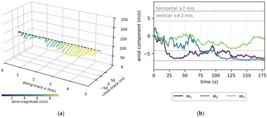
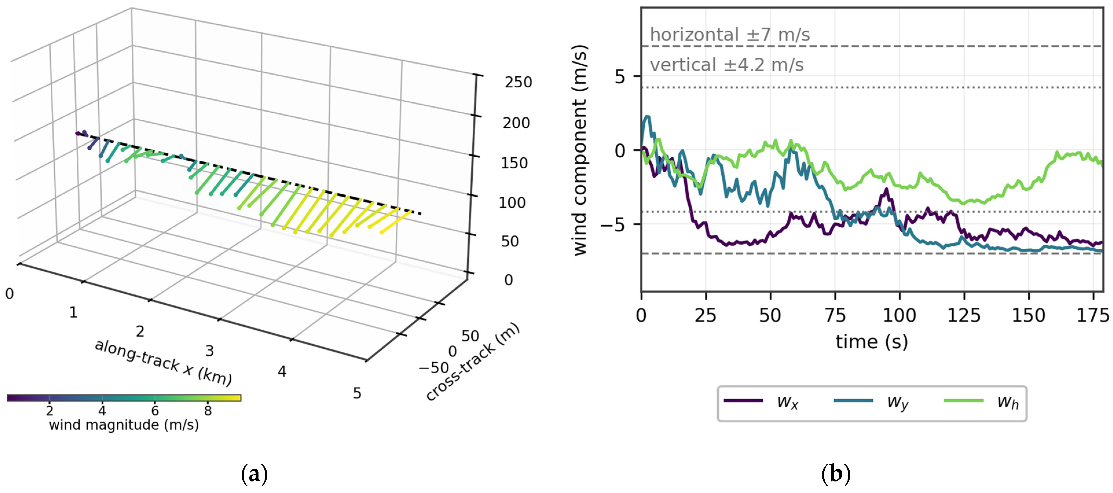
The disturbance and control settings are summarized in Table 3. The slow OU component (τs = 80 s, σs = 5.0 m/s) represents synoptic-scale gusts and the fast component (τf = 10 s, σf = 0.2 m/s) small-scale turbulence; the saturation limit is 7 m/s for the horizontal components and 4.2 m/s for the vertical component, whose standard deviation is scaled to 45% of the horizontal intensity—a gust-dominated field in which the high-frequency component carries only a small fraction of the variance, representative of low-altitude urban operations. The temperature offset and mass factor are drawn per trajectory from [−5,5] K and U(0.95,1.05), and the remaining constants of Equation (2) are ρ0 = 1.225 kg/m3, hs = 8500 m, and T0 = 288.15 K [30]. Figure 4 renders a wind-field realization along a 5 km cruise segment together with the three wind-component time series.
Table 3.
The de disturbance and flight-control settings of the case study.
Figure 4.
The emulated wind field: (a) OU wind vectors along the 5 km cruise segment, drawn in three dimensions, with a common scale of 9 m per m/s on all three axes, so that the direction and length are comparable between stations, but the differing axis spans (5 km along-track, against 130 m cross-track and vertical) must not be read as a faithful quiver (color: wind magnitude; dashed: reference path); and (b) the time series of the three wind components with the horizontal and vertical saturation limits.
3.3. Dataset and Training Configuration
A total of 1000 independent trajectories are generated. The trajectory length varies with the wind, averaging 1106 time steps and spanning 1102 to 1117. With about 45 windows excluded per trajectory at the five phase boundaries (the 10 s input window must lie within a single phase, which removes up to nine windows at each of the five boundaries), each trajectory yields about 1048 samples—1,047,970 in total, of which 2.39% are transition samples. The dataset is partitioned at the trajectory level into 800 trajectories for training, 100 for validation, and 100 for testing (104,791 test samples). The task dimensions of Equation (1) are L = 10 s, H = 5 s, and Δt = 1 s. The network is configured with a hidden dimension d = 128 and contains 266,373 trainable parameters (266,885 for the residual variant); training follows the reproducible protocol in Section 2.6.
4. Results and Discussion
4.1. Realism and Diversity of the Simulated Trajectories
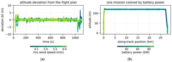
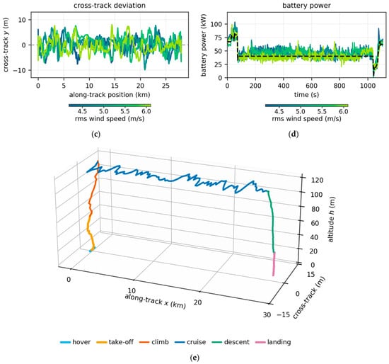
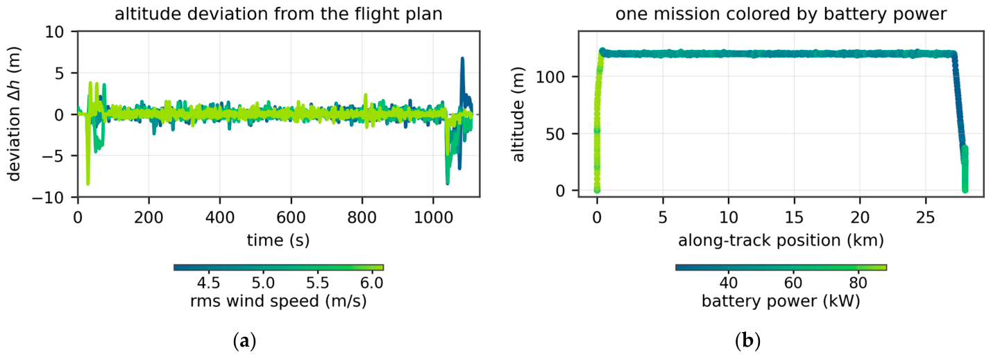
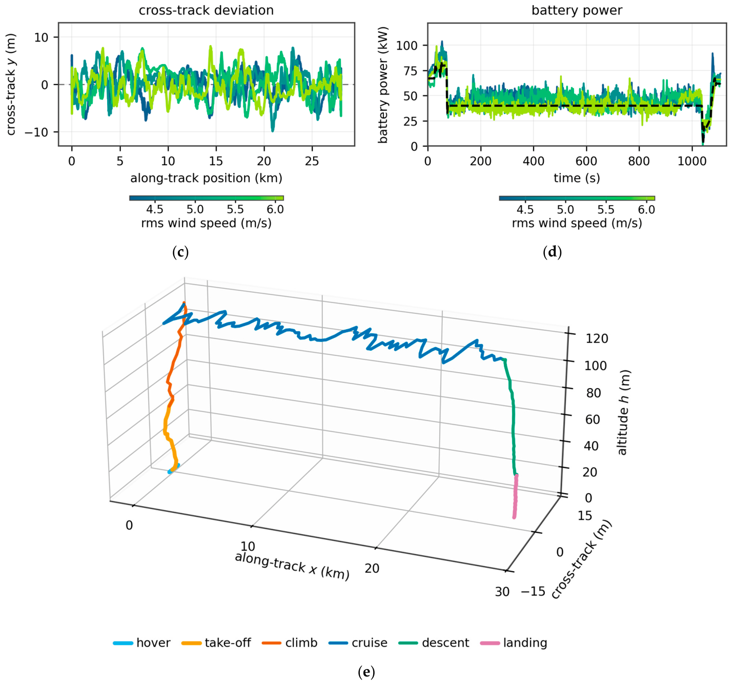
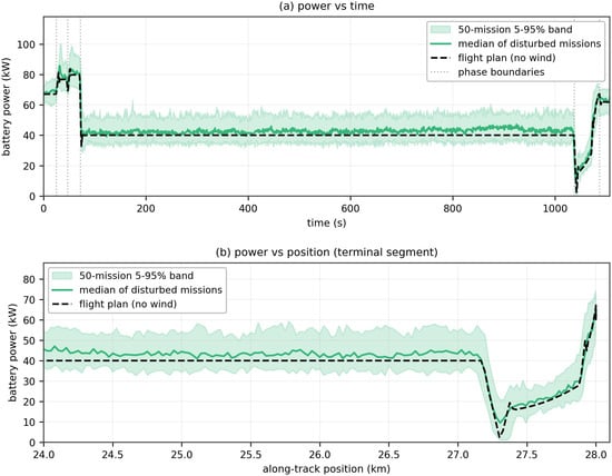
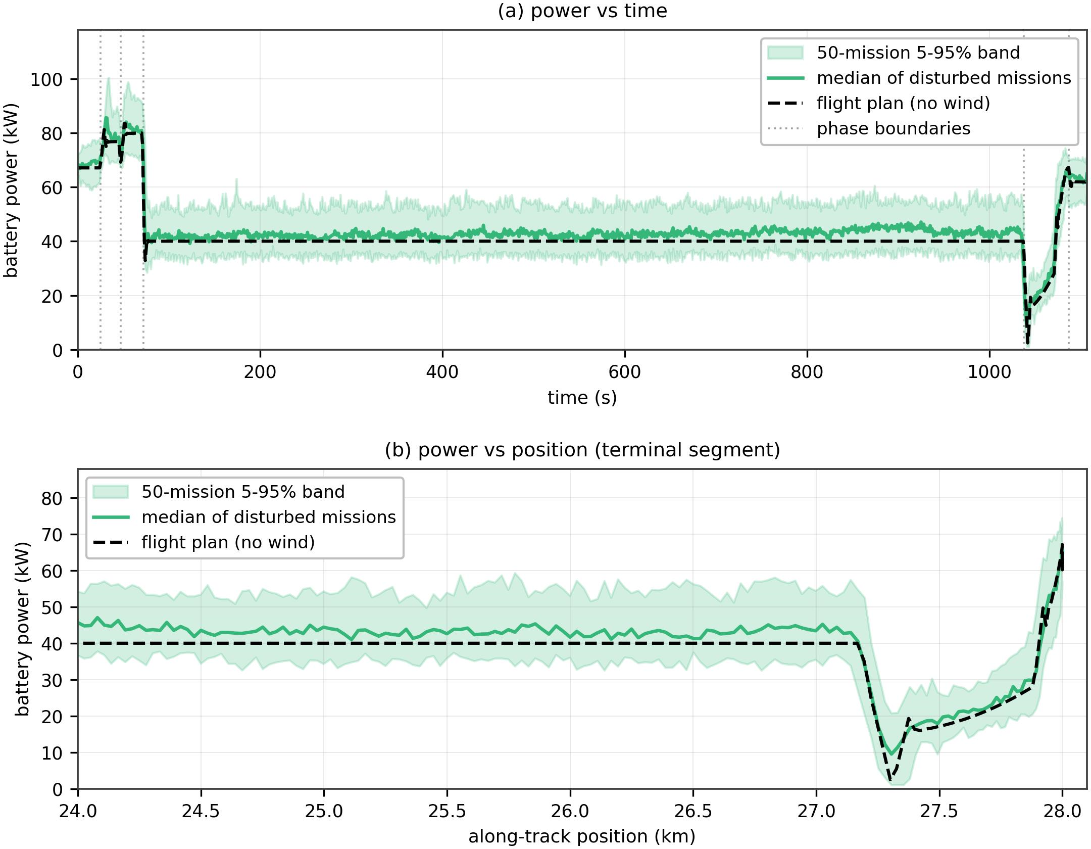
Figure 5 shows simulated 4D trajectories under stochastic wind. Panels (a), (c), and (d) show four trajectories colored by the rms wind speed of their mission, so that a single color scale displays how strongly the wind perturbs the power demand and how far the aircraft is dispersed from the flight plan; panel (b) shows one mission with the battery power encoded as color. Under the emulated control, all trajectories remain tightly bounded to the reference: per-trajectory maximum deviations average 7.3 m (altitude), 8.5 m (cross-track), and 48.9 m (along-track); the corresponding RMS deviations are 0.90, 2.85, and 27.8 m measured against the flight plan at the same instant, and no channel shows sustained oscillation. These are small against the 120 m cruise altitude and the 28.0 km mission distance required of a controlled aircraft under moderate turbulence; the airspeed tracks its reference with an RMS error of 3.71 m/s, and the touchdown point departs from the plan by −20.4 to +25.0 m across the ensemble. The ensemble is also diverse where it matters: the cruise-phase instantaneous power has a 5th–95th percentile range of 33.9–54.4 kW over the 1000-trajectory ensemble, the 50-mission band plotted in Figure 6 spans 34.7–53.6 kW against the nearly constant 40.0 kW reference, and the per-trajectory physics-baseline RMSE varies from 4.85 to 9.55 kW (mean 7.02 kW). Both properties—tight tracking and rich power variability—are prerequisites for the dataset to stand in for flight-test data: a predictor trained on it faces disturbance-induced load excursions of realistic magnitude rather than artifacts of unrealistic trajectory wander, and the tight tracking guarantees that these excursions are attributable to the atmosphere and the control response alone.
Figure 5.
Simulated 4D trajectories under stochastic wind. The four trajectories, selected to span the range of rms wind speed of the ensemble, are colored by the rms wind speed in (a,c,d), so that one color scale shows how the wind intensity shapes the power demand and how far the aircraft departs from the plan. The dashed line marks the wind-free flight plan: (a) the altitude deviation from that plan; (c) the cross-track deviation; and (d) battery power. Panel (b) shows one mission colored by the instantaneous battery power. Panel (e) shows the three-dimensional shape of one simulated mission, colored by flight phase.
Figure 6.
The six−phase power profile: the reference (ideal) power against the median and the 5th–95th percentile band of 50 disturbed trajectories.
4.2. Overall Prediction Performance
Table 4 summarizes the overall RMSE on the held-out test set (100 trajectories, 104,791 samples). The physics baseline attains 7.089 kW—16% of the mean disturbed cruise demand (43.09 kW)—confirming that an idealized onboard model without disturbance feedback is unreliable under realistic turbulence. The stage-average baseline performs 6.7% worse than the physics model (7.564 kW), which is a sharper negative result than a simple comparison suggests: the phase label alone carries almost no predictive value, because the within-phase variability induced by the wind dwarfs the between-phase differences in mean demand. The persistence baseline attains 5.928 kW: exploiting the power signal’s strong short-term autocorrelation, it recovers 16.4% of the physics error yet remains 1.70 times less accurate than the proposed model. The linear-trend baseline attains 6.724 kW. The retained predictor attains 3.483 kW, a 50.9% reduction relative to the physics baseline, while the residual variant attains 3.447 kW. The same predictor attains a mean absolute error of 2.654 kW and a median absolute error of 2.093 kW, with 26.1% of the 523,955 predicted values within 1 kW and 65.5% within 3 kW.
Table 4.
The overall RMSE of the test set and improvement relative to the physics baseline.
Three families of baselines are reported because they answer different questions. The physics model is the same power model that generated the trajectories, evaluated without disturbance feedback; it, therefore, quantifies how far an idealized onboard model of the flight plan falls short under turbulence, rather than whether the learned predictor outperforms a tuned statistical competitor. The stage-average, linear-trend, and persistence baselines are successive sanity checks that use no trajectory information. The remaining entry—an equal-information ridge regression supplied with exactly the same input vector as the LSTM—is the like-for-like comparison: with the information held fixed, it isolates what the learned mapping adds to a linear one. Against the physics model, the retained predictor reduces the RMSE by 50.9%, against the AR(10)+phase ridge by 31.9%, and against the equal-information ridge by 16.9%. The three figures answer different questions and are, therefore, reported together; the last is the most conservative.
Model-based state estimators were also implemented and evaluated under two separate protocols, which must not be compared across. On a 12-trajectory subset with a single-step recursive output, the Kalman filter attains 5.909 kW, the extended Kalman filter 10.319 kW, and moving-horizon estimation 9.104 kW, against 2.266 kW for the proposed predictor on the same subset. On the full test set with the same five-step protocol as the network, the physics-informed hybrid estimator—the analytic model in Section 2.4 used as a trunk with a learned correction—attains 4.199 kW against 3.483 kW. These estimators are not set aside on computational grounds: the Kalman filter is in fact about twelve times faster than the network (0.10 against 1.15 ms per sample). They are set aside by observability. All three are supplied with the same recorded channels as the network—the real-time along-track and cross-track position, the altitude, and the battery power—and the same physical model that generated the data, so they lack neither information nor model structure. What they additionally require is a process model of the disturbance, for which a standard random-walk prior with a smoothing term was used. Because the sensitivity of power to wind enters through the cubic parasite term, inverting the wind from the measured power is ill-conditioned, and a flat smoothing prior necessarily introduces phase lag. The learned predictor avoids that difficulty by regressing directly on a 10 s window of the recorded trajectory and power history, requiring no disturbance prior at all.
All headline results were repeated over three independent weight initializations, with the data and split held fixed. The two-layer plain predictor attains 3.483 ± 0.003 kW (mean ± standard deviation; range 0.007 kW), so the reported RMSE is insensitive to training randomness at the 0.1% level. Because the 104,791 test windows derive from only 100 trajectories, uncertainty was resampled at the trajectory level rather than the sample level: a trajectory-level bootstrap (5000 resamples) gives a 95% confidence interval of [3.446, 3.521] kW for the predictor, and its reduction relative to the physics baseline is [3.425, 3.788] kW, with the predictor more accurate in 100% of resamples. Treating the samples as independent would have narrowed this interval by 78%, which is why the trajectory-level resampling is reported.
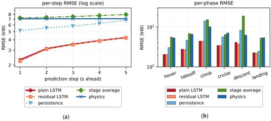
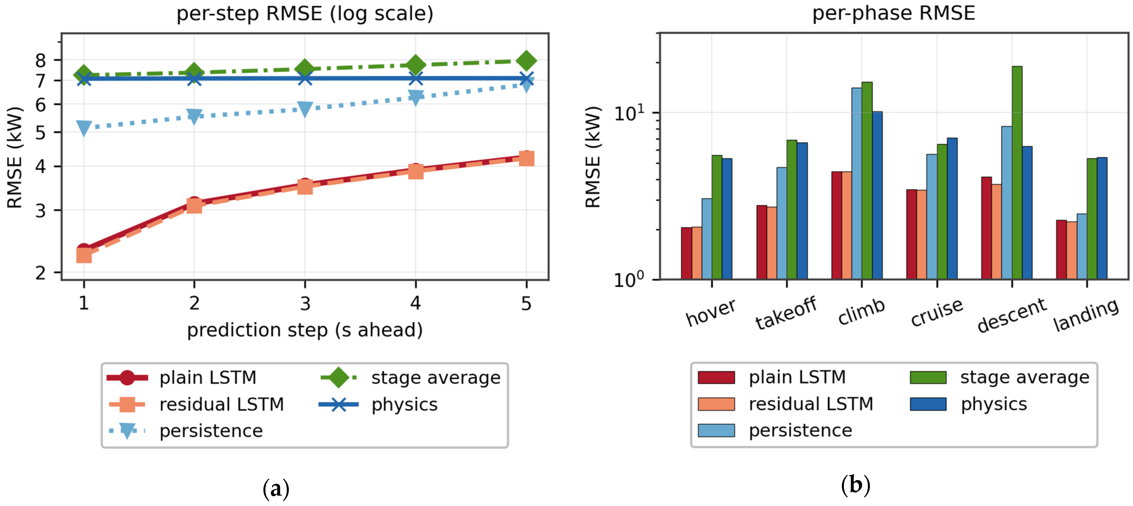
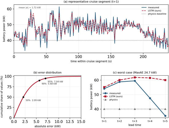
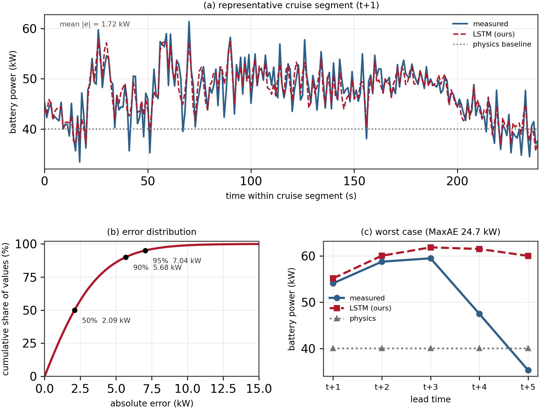
The per-step decomposition (Figure 7a) shows that the error grows gracefully with the lead time, from 2.308 kW at t + 1 to 4.229 kW at t + 5; since all five steps are predicted directly rather than recursively, no error compounding occurs. Persistence is outperformed at every lead time (5.120 kW at t + 1, rising to 6.772 kW at t + 5): even at the shortest horizon, where the autocorrelation it exploits is strongest, its error is 2.22 times that of the LSTM because it cannot anticipate the wind-driven fluctuations already encoded in the power history. The error distribution is strongly concentrated near zero (median 2.093 kW; 95th percentile 7.034 kW), with a right tail that is traced to phase transitions in Section 4.3. Mechanistically, the physics baseline fails because it predicts a nearly constant 40.0 kW cruise power, whereas the true demand has a standard deviation of 6.48 kW and averages 3.1 kW above the plan because the aircraft holds the mean cruise airspeed but not its instantaneous value (standard deviation 3.83 m/s). The excess arises from the control action itself: the power delivered to the rotors is changed only by the pilot, and in this framework, by the emulated pilot, through the airspeed command and the resulting acceleration. Deviations of the instantaneous airspeed from its mean (standard deviation 3.83 m/s) are, therefore, the visible trace of that action rather than an independent cause. Decomposing the cruise-phase power over the test set confirms this: the parasite term contributes +77% of the variance, the non-regenerative acceleration term +25%, and the potential-energy term +25%, while the induced term partially cancels them at −27%, so that the net airspeed sensitivity is only 1.15 kW per (m/s) and airspeed alone accounts for 4.39 kW of the 6.48 kW. The power-history channel lets the LSTM exploit precisely this: the trace of the pilot’s action is already present in the recent power signal.
Figure 7.
The test-set RMSE of the predictors: (a) the per-prediction step; and (b) the per-flight phase (both panels use a logarithmic ordinate).
These numbers translate directly into battery-safety, airworthiness, and fleet-dispatch terms. For the battery management system (BMS), the error statistics size the short-term power reserve: an estimator built on the idealized model would deviate from the mean cruise demand by 16% and must absorb power swings with a 5th–95th percentile range of 33.6–54.2 kW on the held-out test set that its profile-based estimate cannot anticipate, whereas the proposed predictor’s 3.483 kW RMSE is 8.1% of the 43.09 kW mean cruise demand and stays within 7.04 kW (16.3%) for 95% of the test samples—reserve margins can be tightened accordingly without loss of safety coverage. Because the load excursions are driven by gusts with an 80 s correlation time, while the prediction is available five seconds ahead, the forecast gives the BMS actionable lead time for current-limit scheduling and thermal preconditioning against the repeated high-rate discharge that drives cell aging and thermal risk [3,5]. For airworthiness, the empirical 95th-percentile error bound converts the qualitative requirement of in-flight power-margin monitoring into a sized, monitorable margin. Finally, aggregated across a fleet, second-level forecasts of this accuracy are precisely the input that vertiport charging scheduling and eVTOL–grid co-optimization currently have to assume rather than predict [17,18].
4.3. Per-Phase and Transition Errors
Figure 7b breaks the RMSE down by the flight phase. The cruise phase contributes 91.17% of all of the test samples and, therefore, dominates the overall metric; the retained predictor attains 3.470 kW, about half the physics baseline (7.100 kW). The climb phase is the most difficult phase for the learning model and for the physics baseline alike (4.446 kW against 10.167 kW), despite its small sample share: the reference airspeed ramps continuously from 0 to 27.78 m/s within the climb, so the aerodynamic state changes substantially within a single 10 s input window and the acceleration-dependent power terms are most active. The ordering of the remaining phases is consistent between the two: descent (4.134 kW) and take-off (2.798 kW) are intermediate, while hover (2.065 kW) and landing (2.273 kW) are the least difficult. Persistence is worst in climb (14.077 kW), worse even than the physics model’s 10.167 kW, its constant-power assumption being maximally violated under the speed ramp. Hover is estimated from 1100 in-phase test windows rather than from a single phase-crossing sample.
Transition samples—whose five label steps cross a phase boundary—constitute 2.39% of the test set (2500 samples) and remain more difficult: the transition RMSE (4.685 kW) is 1.36 times the in-phase RMSE (3.449 kW), and their dominance grows towards the tail. Although they are only 2.4% of the samples, they account for 27% of the absolute errors above 15 kW and 71% of those above 22 kW. Two mechanisms compound: the reference vertical rate changes at the boundary, and the emulated controller responds with a corrective transient that temporarily couples all three channels, whereas the input window contains only pre-transition information by construction. The learning model nevertheless copes far better than the physics baseline because the approach to a boundary is partly observable from the state itself—the input includes the remaining distance to the next phase trigger (Section 2.1)—and on representative windows, including the worst case, the prediction tracks the power change with only a small delay and amplitude error. Practically, phase transitions are scheduled, flight-plan-known events, so an onboard system can raise its alert level at these instants; across the whole flight, the absolute error stays below 3 kW for 65.5% of the samples and below 10 kW for 98.9% of them.
The engineering reading of this error structure is favorable to deployment. With the boundary-remaining channel in the input (Section 2.1), the transition samples are no longer the source of the largest errors, although they still dominate the error tail: transition samples are 2.39% of the test set and contribute 4.3% of the total squared error, so the difficulty they posed to the earlier input design has largely been removed. The largest single residual of the test set (24.722 kW) occurs instead inside the cruise phase at the fifth lead time of a window, in which the measured power falls by about 19 kW within five seconds—a gust excursion that no model with a 5 s horizon anticipates from a 10 s history (Figure 8c). For certification, this matters in two ways: the predictor’s uncertainty budget is close to uniform over the mission, with an absolute error below 10 kW for 98.9% of the samples, and the transitions that remain the hardest are scheduled, flight-plan-known events that operational procedures can flag—a substantially easier assurance case than an uncharacterized, unbounded error.
Figure 8.
Prediction against measurement on the held-out test set: (a) a representative cruise segment showing the measured battery power, the predictor, and the physics baseline at the first lead time; (b) the cumulative distribution of the absolute error over all 523,955 predicted values, with the 50th, 90th, and 95th percentiles marked; and (c) the worst case of the test set (24.722 kW at t + 5), in which the measured power falls by about 19 kW within five seconds. Here and throughout, the forecast horizon is 5 s and the input window is 10 s.
4.4. Ablation Study
Two ablations isolate the sources of performance, beginning with the input design. Within the cruise segment, power correlates strongly with airspeed (Pearson r = 0.669), as the aerodynamic model requires, but is uncorrelated with groundspeed (r = −0.022)—the latter being the only quantity inferable from position records. Across the whole mission, the correlation reverses sign because hover draws high power at zero speed while cruise draws less at high speed, so it is quoted within the cruise segment. Since the wind, and hence the airspeed for a given ground track, is unobservable from the 4D trajectory, the power history is the input channel through which the network can infer the prevailing air-relative flow state. Masking this channel—by zeroing it in the input while leaving the architecture, the parameter count (266,373), and the training budget unchanged—raises the overall RMSE from 3.483 kW to 5.815 kW, a 1.67-fold increase that leaves the masked model at essentially the same accuracy as the persistence baseline (5.928 kW) and only 18% ahead of the idealized physics model. The masked model’s per-step RMSE still grows with the lead time (5.474 to 6.019 kW) and remains 1.4 to 2.4 times that of the full model at every step. The power history thus carries the decisive information that the trajectory itself lacks—the central empirical justification of the input design.
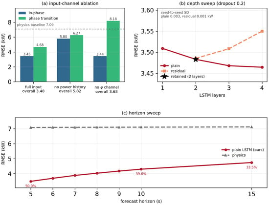
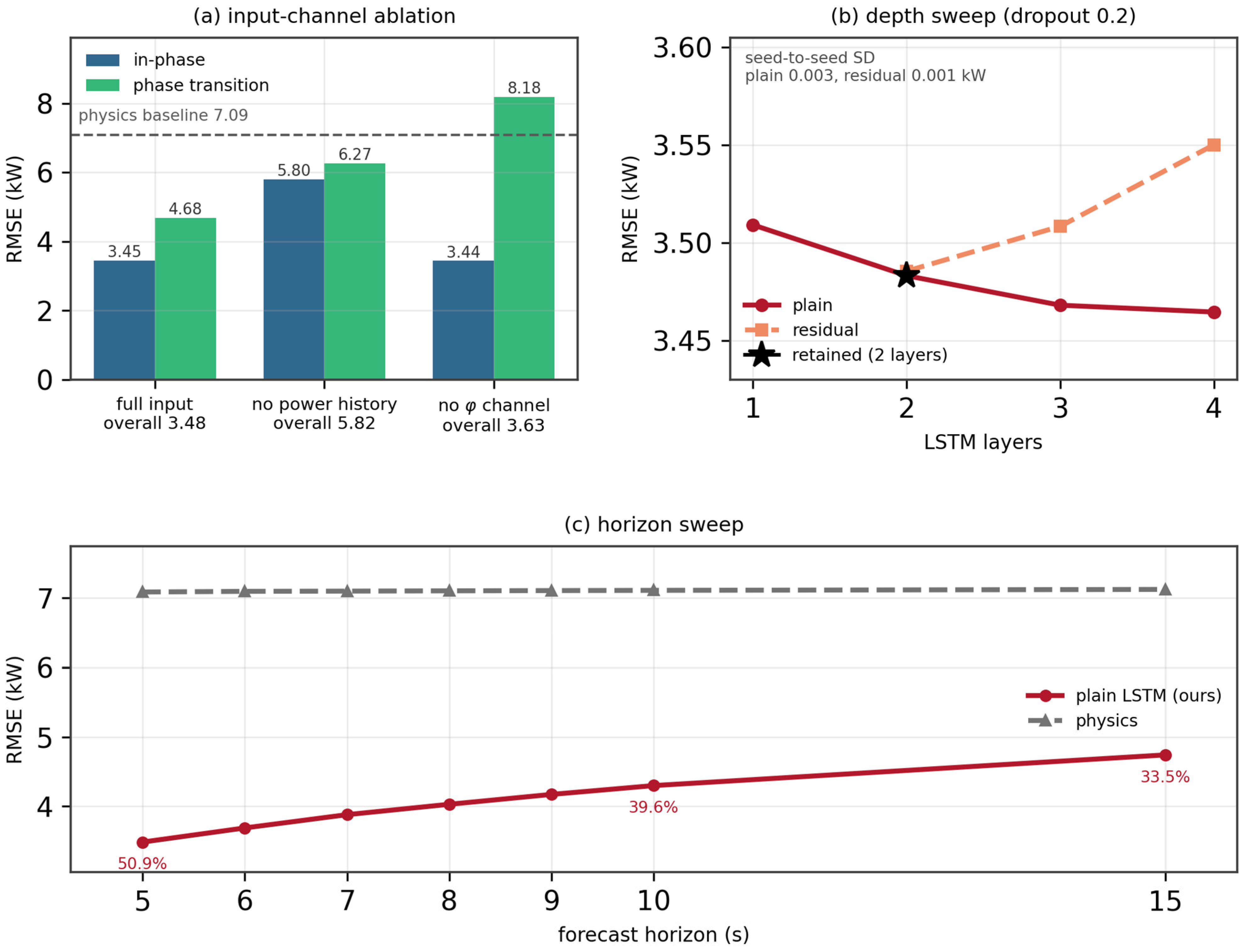
A third ablation isolates the fifth physical channel, the distance remaining to the next phase-trigger boundary. Re-running the identical pipeline with that channel removed, while keeping the same dataset, split, seed, epoch budget, and architecture, with the input dimension changing from 11 to 10 and the parameter count from 266,373 to 266,245, raises the overall RMSE from 3.483 to 3.627 kW and the transition-sample RMSE from 4.685 to 8.183 kW, a 42.8% reduction attributable to that single channel, while the in-phase RMSE is essentially unchanged (3.449 against 3.441 kW, +0.2%). The maximum absolute error rises from 24.722 to 44.749 kW. The effect is, therefore, confined to exactly the samples the channel describes, which is the mechanism claimed in Section 2.1: because the along-track coordinate is window-relative, a position-triggered boundary is invisible until it has been crossed. Panels (a) and (b) in Figure 9 summarize this and the depth sweep below.
Figure 9.
Ablations. (a) The overall, in-phase, and transition RMSE for the full input, with the power-history channel removed and with the φ channel removed, against the physics baseline. (b) Depth sweep for both families under a common dropout rate of 0.2, with the retained two-layer configuration marked and the seed-to-seed standard deviation annotated. (c) The RMSE against the forecast horizon for the predictor and the physics baseline, with the relative reduction annotated at 5, 10, and 15 s.
The second ablation sweeps both network families from one to four layers under unchanged per-family training protocols (Figure 9b), and the aerodynamic and temporal structure of the task explains the outcome. Physically, the mapping to be learned is quasi-steady: momentum theory (Section 2.4) is instantaneous, so the future power is determined by the current aerodynamic state—airspeed, climb rate, and the prevailing wind—while the only genuine dynamics are the 3 s first-order airspeed response and the OU gust evolution (correlation times 10–80 s against a 10-step window). A 10 s window of trajectory and power history, therefore, already measures the state of this low-order system, which is why the plain family is essentially insensitive to depth: across one to four layers, its RMSE spans 3.465 to 3.509 kW, a range of 1.3%. A single recurrent layer already captures most of the learnable mapping, and additional layers add parameters but no missing function class. Temporally, the task unrolls only ten steps—far shorter than the horizons LSTM gating was designed for [32]—so the depth-related gradient pathology that residual connections were introduced to cure [33] does not manifest for the plain model. The residual wrapper, by contrast, gains nothing from the depth: with the dropout rate held at 0.2 for both families, it is equivalent to the plain model at two layers (3.4855 against 3.4832 kW, a gap of +0.002) and worse at three and four layers (+0.040 and +0.086 kW). Two effects are consistent with this: post-block layer normalization re-standardizes the hidden activations whose magnitude encodes the power level that the next layer’s gates exploit, and per-block dropout injects regularization noise into a regression problem, with 838,367 training windows against 266,373 parameters, where overfitting pressure is negligible, and the added variance can only hurt. The residual variant listed in Table 4 owes its marginally lower RMSE to its lower dropout rate (0.1 against 0.2) rather than to the residual connections: under a matched dropout rate and training budget, the two families are equivalent at two layers. Overall, architecture choices alter the accuracy by at most 1.3%, whereas the input design alters it by 66%: the predictive content of this task resides in the input channels, and the practical recommendation is a shallow plain LSTM, which is also the simplest to verify. A single random seed was used throughout the sweep, so these differences should be read as descriptive rather than as significance tests. The relevant distinction is that the underlying aerodynamic relation is quasi-steady—an algebraic function of the instantaneous airspeed, climb rate, and wind—so the network need not integrate any dynamics. What it must do is reconstruct the unobserved relative airflow state from the recent power response, which is why the power-history channel is decisive (Section 4.4).
For the plain family, the error does improve slightly with depth—from 3.483 kW at two layers to 3.468 kW at three and 3.465 kW at four, a total gain of 0.019 kW (0.5%) for twice the parameters—but that gain amounts to 0.5% of the RMSE, and the two-layer configuration is retained as the final predictor for its smaller size and simpler verification surface. Figure 9b shows both families over the full depth sweep.
For onboard deployment, this is a favorable outcome. The recommended predictor is a two-layer network of 266,373 parameters with direct multi-step output—no recurrence at inference, no residual branches, and no normalization layers—whose inference cost is about 1.15 ms per sample on a desktop CPU and negligible relative to flight-computer budgets, and whose shallow, homogeneous structure and purely feed-forward evaluation simplify the verification effort that the assurance of learning-based airborne components requires.
Finally, the sensitivity to the prediction horizon is examined by extending the output length, while keeping the ten-step input window unchanged. Predicting ten steps raises the overall RMSE to 4.299 kW against 7.112 kW for the physics baseline on the same labels—a reduction of 39.6%, compared with 50.9% at the five-step horizon—and predicting fifteen steps gives 4.741 kW against 7.126 kW, a reduction of 33.5%. The first five lead times of the ten-step model reproduce the main experiment within 2.7%, and the per-step error of the fifteen-step model grows from 2.399 kW at the first step to 5.607 kW at the fifteenth, with monotonically decreasing increments (0.776 kW between the first two steps and 0.038 kW between the last two). The cumulative error, therefore, grows sub-linearly with the lead time rather than accumulating. Over the range examined here—5, 10, and 15 s—the overall RMSE rises from 3.483 to 4.741 kW, i.e., the framework degrades gracefully, rather than catastrophically, as the look-ahead requirement grows.
4.5. Limitations and Future Work
Several limitations bound these results, the foremost being that all of the conclusions are drawn from simulation. The present work is, however, a design-stage study by construction: it asks whether the battery power load of an eVTOL aircraft over the next few seconds can be predicted from its four-dimensional trajectory, and it addresses that question under conditions that are controlled, reproducible, and systematically variable—which is what a design-stage study requires, since at that stage the aircraft configuration, the mission profile, and the disturbance environment are precisely the quantities that are to be explored. The staged plan below, therefore, sets out how the framework is to be carried forward in subsequent work. First, the simulator itself should be recalibrated against flight-test telemetry—identifying the product Cd·Af (the two factors are not separately identifiable), η, and Paux from the recorded data—so that the model-form component of the sim-to-real gap is shrunk before any predictor is retrained. Second, the simulation-pretrained network can be fine-tuned on operational recordings at a reduced learning rate: the domain randomization already built into the generator (mass ±5%, temperature ±5 K, and wind spectrum) widens the training envelope so that real data are more likely to lie inside it, and the power-history input is precisely the channel that absorbs residual mismatch, since it carries the aircraft’s actual power response rather than a modeled one. Third, where a systematic offset remains, a small bias-correction model can be learned on the simulated-versus-measured residual as real data accumulate. And fourth, validation should proceed progressively from hardware-in-the-loop tests to a structured flight-test campaign. All predictor inputs—4D track, battery power, and flight phase—are standard recorded telemetry, so no sensor retrofit is required for deployment.
Research with real flight data is accordingly the next stage of this work. The framework is presented here as a prospective, design-stage capability: its power model, disturbance emulation, data-generation chain, and evaluation protocol are specified completely enough that the staged path above can be executed as soon as operational recordings from an aircraft of this class are available, and carrying the framework over to real data is the immediate outlook of this work.
Two further limitations concern the scope. The power model captures the aerodynamic and propulsive demand but not battery electrochemical dynamics (state-of-charge dependence, voltage sag, and thermal derating), assumes a constant auxiliary floor, and credits no regenerative recovery; coupling the demand model to an electrochemical pack model is the natural next step toward a full energy-management loop. A single aircraft type and mission profile are considered, and the stationary OU wind represents neither gust fronts nor thermals. The aerodynamic model also lumps the parasite term into a single orientation-independent drag coefficient and the rotor losses into one propulsive efficiency; a formulation in which the drag coefficient depends explicitly on the angle of attack and sideslip would refine the cruise estimates and will be pursued alongside the higher-fidelity simulator described above. Future work will execute the transfer plan above, extend the predictor to calibrated probabilistic forecasting, and investigate phase-specific heads and alternative sequence models.
5. Conclusions
This paper addressed the prediction of the near-future battery output power of an eVTOL aircraft from four-dimensional trajectory data. A simulation platform developed around the certified EHang 216-S multirotor—a six-phase reference profile, steady-state-variance Ornstein–Uhlenbeck wind with smooth saturation, temperature and mass randomization, and three-channel flight-control emulation—generated 1,047,970 supervised samples from 1000 missions, and a unified rotor momentum-theory power model, evaluated identically for reference and disturbed trajectories with the air-relative climb rate in the axial balance and the inertial rate in the potential-energy term, ensures that the physics–baseline error reflects genuine disturbance effects. The reference mission stays inside the aircraft’s certified envelope of 200 m above ground level, 30 km, and 25 min, and consumes 13.0 kWh of the 31 kWh battery.
On the held-out test set, the physics baseline attains an 7.089 kW RMSE (about 16% of the mean disturbed cruise demand) and the stage-average baseline is 6.7% worse still (7.564 kW), whereas the retained predictor estimates the next 5 s from a 10 s trajectory-and-power window at 3.483 kW—a 50.9% reduction relative to the physics model, and 16.9% against a linear predictor given exactly the same inputs—with the error concentrated near zero (median 2.093 kW) and the error tail still dominated by phase transitions, while the single largest residual occurs inside the cruise phase (transition RMSE 4.685 versus 3.449 kW in-phase); phase transitions are scheduled, flight-plan-known events and can be flagged operationally. Ablations show the power-history input to be decisive (masking it degrades the RMSE to 5.815 kW, i.e., to the level of persistence, consistent with a cruise-segment power–airspeed correlation of 0.669 against −0.022 for groundspeed), a shallow plain model to be sufficient (depth sweep 3.465–3.509 kW), and the residual variant to be equivalent to the plain model under a matched dropout rate and budget; extending the horizon to 10 and 15 s preserves 39.6% and 33.5% reductions, with sub-linear error growth. The distance to the next phase-trigger boundary, available on board from the pre-loaded flight plan, is what makes the transitions tractable.
Positioned against prior work, verified eVTOL design tools achieve mission-energy accuracy of about 10% under nominal conditions [10], and learning-based energy prediction has reached high accuracy at flight or trip resolution in adjacent domains [14,15]. The present results quantify what such nominal-condition models imply at second-level resolution—an error of about 16% of the mean disturbed cruise demand under moderate turbulence—and show that a trajectory- and power-history-driven predictor halves it. To the authors’ knowledge, this is the first study to predict the second-level battery power load of an eVTOL aircraft from 4D trajectory data under emulated disturbances. The framework offers a practical basis for design-stage battery sizing, predictive battery management with an empirical 95th-percentile error bound, and the fleet-level load forecasts presupposed by eVTOL scheduling and grid co-optimization [17,18]; future work will validate it on real flight data following the staged transfer plan in Section 4.5, couple the demand model with battery electrochemical dynamics, and extend the predictor to calibrated probabilistic forecasting.
Author Contributions
Conceptualization, Y.Y., and R.L.; methodology, Y.Y., R.L. and C.S.L.; software, R.L.; validation, Y.Y., R.L.; formal analysis, Y.Y. and R.L.; investigation, Y.Y., D.H., and C.S.L.; resources, Y.Y., C.S.L. and G.T.; data curation, R.L.; writing—original draft preparation, Y.Y., R.L., and C.S.L.; writing—review and editing, D.H. and G.T. All authors have read and agreed to the published version of the manuscript.
Funding
This work is supported by the Open Fund of the Civil Aviation University of China under Grant GY202605.
Data Availability Statement
The raw data supporting the conclusions of this article will be made available by the authors on request.
Conflicts of Interest
The authors declare no conflict of interest.
Abbreviations
| Symbol | Definition | Symbol | Definition |
| ri = (ti, xi, yi, hi) | 4D trajectory sample | Prot, Paero | Rotor shaft/aerodynamic power |
| Δt | Sampling interval | Pgrav, Pacc | Potential-energy/acceleration power |
| Actual/predicted battery power | Paux | Auxiliary power | |
| ci,e(ci) | Phase index/one-hot encoding | Va, Vg | Airspeed/groundspeed |
| L, H | Input window/prediction horizon | V*, h* | Nominal cruise speed/altitude |
| fθ | Learned predictor | FT | Rotor thrust |
| Xt,yt | Input tensor/label vector | vh, vi | Hover/climbing induced velocity |
| N | Number of samples | vc, vc,g | Air-mass-relative/inertial climb rate |
| m0, ξm | Nominal mass/mass factor | W | Aircraft weight |
| Nr, Dp, A | Rotor number/diameter/disk area | nl | Load factor |
| Cd, Af | Drag coefficient/frontal area | aa, alat | Longitudinal/lateral acceleration |
| η | Propulsive efficiency | w, wmax | Wind speed/saturation limit |
| ρ, δT | Air density/temperature offset | τ, σ, α | OU correlation time/standard deviation/coefficient |
| d | Hidden dimension | RMSE, MAE | Root-mean-square/mean absolute error |
| U | Free-stream speed normal to rotor disk | β, τp | Low-pass coefficient/control bandwidth |
| Filtered/raw control command | Tracking error/error rate/integrator state | ||
| φ | Remaining distance to the next phase Boundary, as a fraction of the phase span |
References
- Zhao, L.; Chen, Y.; Wahab, M.I.M. The impact of low-altitude airspace opening policy on aviation manufacturing innovation: A double machine learning approach. Transp. Res. Part A Policy Pract. 2025, 200, 104660. [Google Scholar] [CrossRef] [Scilit]
- Dixit, M.; Bisht, A.; Witherspoon, B.; Essehli, R.; Amin, R.; Duncan, A.; Hines, J.; Kweon, C.-B.M.; Belharouak, I. Battery electrolyte design for electric vertical takeoff and landing (eVTOL) platforms. Adv. Energy Mater. 2024, 14, 2400772. [Google Scholar] [CrossRef] [Scilit]
- Yang, X.-G.; Liu, T.; Ge, S.; Rountree, E.; Wang, C.-Y. Challenges and key requirements of batteries for electric vertical takeoff and landing aircraft. Joule 2021, 5, 1644–1659. [Google Scholar] [CrossRef] [Scilit]
- Viswanathan, V.; Epstein, A.H.; Chiang, Y.-M.; Takeuchi, E.; Bradley, M.; Langford, J.; Winter, M. The challenges and opportunities of battery-powered flight. Nature 2022, 601, 519–525, Correction in Nature 2022, 603, E30. https://doi.org/10.1038/s41586-022-04612-5. [Google Scholar] [CrossRef] [Scilit] [PubMed]
- Sripad, S.; Bills, A.; Viswanathan, V. A review of safety considerations for batteries in aircraft with electric propulsion. MRS Bull. 2021, 46, 435–442. [Google Scholar] [CrossRef] [Scilit]
- Donateo, T.; Ficarella, A. A methodology for the comparative analysis of hybrid electric and all-electric power systems for urban air mobility. Energies 2022, 15, 638. [Google Scholar] [CrossRef] [Scilit]
- Donateo, T.; Spada Chiodo, L.; Ficarella, A.; Lunaro, A. Improving the dynamic behavior of a hybrid electric rotorcraft for urban air mobility. Energies 2022, 15, 7598. [Google Scholar] [CrossRef] [Scilit]
- Fay, T.-A.; Semmler, F.-B.; Cigarini, F.; Göhlich, D. Feasibility Study of Current and Emerging Battery Chemistries for Electric Vertical Take-Off and Landing Aircraft (eVTOL) Applications. World Electr. Veh. J. 2025, 16, 137. [Google Scholar] [CrossRef] [Scilit]
- He, R.; Holzapfel, F.; Bröcker, J.; Lai, Y.; Zhang, S. A Decentralized Voting and Monitoring Flight Control Actuation System for eVTOL Aircraft. Aerospace 2024, 11, 195. [Google Scholar] [CrossRef] [Scilit]
- Yanev, R.Y.; Staack, I. Framework for rapid eVTOL aircraft configuration design: Methodology and verification. Aerospace 2026, 13, 566. [Google Scholar] [CrossRef] [Scilit]
- Yuan, J.; Zhu, Z.; Zhang, H. Power consumption modeling and analysis of low-altitude eVTOL for urban air mobility. In Proceedings of the 2025 IEEE Transportation Electrification Conference and Expo, Asia-Pacific (ITEC Asia-Pacific); IEEE: Piscataway, NJ, USA, 2025; pp. 1–6. [Google Scholar] [CrossRef] [Scilit]
- Zhang, J.; Söpper, M.; Holzapfel, F.; Zhang, S. Four-Dimensional Generalized AMS Optimization Considering Critical Engine Inoperative for an eVTOL. Aerospace 2024, 11, 990. [Google Scholar] [CrossRef] [Scilit]
- Sisk, S.; Du, X. Surrogate-Based Multidisciplinary Optimization for the Takeoff Trajectory Design of Electric Drones. Processes 2024, 12, 1864. [Google Scholar] [CrossRef] [Scilit]
- Selje, R.A.; Rubio, R.; Gorospe, G.E.; Sun, L. Comprehensive study of machine learning techniques to predict flight energy consumption for advanced air mobility. In Proceedings of the AIAA SCITECH 2024 Forum; Paper No. 0534; AIAA: Reston, VA, USA, 2024. [Google Scholar] [CrossRef] [Scilit]
- Dong, C.; Xiong, Z.; Zhang, C.; Li, N.; Li, Y.; Xie, N.; Zhang, J.; Wang, H. A transformer-based approach for deep feature extraction and energy consumption prediction of electric buses based on driving distances. Appl. Energy 2025, 380, 123941. [Google Scholar] [CrossRef] [Scilit]
- Xu, Y.; Pan, Q.; Wang, Z.; Hu, B. A novel trajectory prediction method based on CNN, BiLSTM, and multi-head attention mechanism. Aerospace 2024, 11, 822. [Google Scholar] [CrossRef] [Scilit]
- Yuan, Y.; Li, J.; Zhao, X.; Wang, Y. eVTOL scheduling schemes for dynamic demand and variable intervals. Acta Aeronaut. Astronaut. Sin. 2026, 47, 631907. (In Chinese) [Google Scholar] [CrossRef]
- Yuan, Y.; Lai, C.S.; Chi, H.R.; Wang, H.; Tsang, K.F. Power systems and eVTOL optimization with information exchange for green and safe urban air mobility. Sensors 2026, 26, 888. [Google Scholar] [CrossRef] [Scilit] [PubMed]
- Yeh, S.-T.; Du, X. Transfer-Learning-Enhanced Regression Generative Adversarial Networks for Optimal eVTOL Takeoff Trajectory Prediction. Electronics 2024, 13, 1911. [Google Scholar] [CrossRef] [Scilit]
- Wang, Y.; Li, J.; Yuan, Y.; Lai, C.S. Joint optimization of cost and scheduling for urban air mobility operation based on safety concerns and time-varying demand. Aerospace 2024, 11, 861. [Google Scholar] [CrossRef] [Scilit]
- Civil Aviation Administration of China. Special Conditions for the EHang EH216-S Unmanned Aircraft System (SC-21-002); CAAC: Beijing, China, 2022.
- European Union Aviation Safety Agency. Notice of Proposed Amendment 2026-01: Regular Update of the Aerodrome Rules for the Transposition of ICAO SARPs Amendments; EASA: Cologne, Germany, 2026.
- European Union Aviation Safety Agency. Means of Compliance with the Special Condition VTOL (MOC-2 SC-VTOL); EASA: Cologne, Germany, 2021.
- Federal Aviation Administration. Engineering Brief No. 105A: Vertiport Design; U.S. Department of Transportation: Washington, DC, USA, 2024.
- Kim, S.; Park, O.; Shin, H.-S. A Design of VFR Approach and Departure Procedures of UAM at Vertiports Adjacent to the Airport. In Proceedings of the 34th Congress of the International Council of the Aeronautical Sciences (ICAS 2024), Florence, Italy, 9–13 September 2024. Paper ICAS2024-0110. [Google Scholar]
- Qanbari, A.; Skorupski, J. Scalability of eVTOL Systems: Insights from Multi-Pad Configurations and CPN Analysis. Aerospace 2025, 12, 147. [Google Scholar] [CrossRef] [Scilit]
- Song, K. Optimal Vertiport Airspace and Approach Control Strategy for Urban Air Mobility (UAM). Sustainability 2023, 15, 437. [Google Scholar] [CrossRef] [Scilit]
- Clarke, M.A.; Alonso, J.J. Evaluating the Performance and Acoustic Footprint of Aircraft for Regional and Urban Air Mobility. In Proceedings of the AIAA AVIATION 2021 Forum; Paper AIAA 2021-3205; American Institute of Aeronautics and Astronautics (AIAA): Reston, VA, USA, 2021. [Google Scholar] [CrossRef] [Scilit]
- Beyne, E.E.A.; Castro, S.G.P. Preliminary Performance Assessment of a Long-Range eVTOL Aircraft. In Proceedings of the AIAA SciTech 2022 Forum; Paper AIAA 2021-3205; American Institute of Aeronautics and Astronautics (AIAA): Reston, VA, USA, 2022. [Google Scholar] [CrossRef] [Scilit]
- National Oceanic and Atmospheric Administration; National Aeronautics and Space Administration; United States Air Force. U.S. Standard Atmosphere, 1976; U.S. Government Printing Office: Washington, DC, USA, 1976.
- Johnson, W. Helicopter Theory; Princeton University Press: Princeton, NJ, USA, 1980. [Google Scholar]
- Hochreiter, S.; Schmidhuber, J. Long short-term memory. Neural Comput. 1997, 9, 1735–1780. [Google Scholar] [CrossRef] [Scilit] [PubMed]
- He, K.; Zhang, X.; Ren, S.; Sun, J. Deep residual learning for image recognition. In Proceedings of the IEEE Conference on Computer Vision and Pattern Recognition; IEEE: Piscataway, NJ, USA, 2016; pp. 770–778. [Google Scholar] [CrossRef] [Scilit]
- Ba, J.L.; Kiros, J.R.; Hinton, G.E. Layer normalization. arXiv 2016, arXiv:1607.06450. [Google Scholar] [CrossRef] [Scilit]
- Srivastava, N.; Hinton, G.; Krizhevsky, A.; Sutskever, I.; Salakhutdinov, R. Dropout: A simple way to prevent neural networks from overfitting. J. Mach. Learn. Res. 2014, 15, 1929–1958. [Google Scholar]
- Kingma, D.P.; Ba, J. Adam: A method for stochastic optimization. arXiv 2014, arXiv:1412.6980. [Google Scholar] [CrossRef] [Scilit]
- Académie de l’Air et de l’Espace. eVTOL: An Overview; AAE Dossier No. 53; AAE: Paris, France, 2022; Available online: https://academieairespace.com/evtol-un-tour-dhorizon/?lang=en (accessed on 26 September 2026).

Disclaimer/Publisher’s Note: The statements, opinions and data contained in all publications are solely those of the individual author(s) and contributor(s) and not of MDPI and/or the editor(s). MDPI and/or the editor(s) disclaim responsibility for any injury to people or property resulting from any ideas, methods, instructions or products referred to in the content. |
© 2026 by the authors. Licensee MDPI, Basel, Switzerland. This article is an open access article distributed under the terms and conditions of the Creative Commons Attribution (CC BY) license.